Impact of mesoscale eddy parameterization on Arctic Atlantic Water circulation and heat transport in the eddy-permitting grey zone

The Arctic Ocean is undergoing rapid change, yet many CMIP-type climate models struggle to accurately represent its circulation and water masses. A key feature of the system is the topographically controlled boundary currents that transport warm, saline Atlantic Water northward at intermediate depths into the Atlantic Water layer. An important process affecting these boundary currents is the lateral flux of heat and salt driven by mesoscale eddies. Because the deformation radius is relatively small in the Arctic Ocean, numerical simulations require kilometer-scale resolution to fully capture eddy dynamics. Most of the current climate models, however, operate in a non-eddying regime, relying on mesoscale eddy parameterizations – typically combining isopycnal diffusion (Redi) with eddy-induced advection (Gent and McWilliams, GM). As horizontal resolution increases, future models will shift from an eddy-parameterized to eddy-permitting regime, entering a grey zone where eddies are only partially resolved and the role of GM parameterization becomes less straightforward. This study investigates the use of GM parameterization in eddy-permitting models, focusing on its effect on the northward transport of Atlantic Water in the Nordic Seas and Arctic Ocean. We conduct realistic simulations where we vary GM diffusivity strength and test two different GM scalings. These experiments are compared with a high-resolution reference simulation and observational data. Further, we show how the GM parameterization modulates the topographically steered boundary current through a reduction in baroclinicity of the large-scale circulation, how transport across Greenland–Scotland Ridge and Fram Strait is controlled by its strength; and how resolved and parameterized eddy heat fluxes contribute to the redistribution of heat. Our results suggest that mesoscale eddy buoyancy fluxes remain insufficiently resolved at eddy-permitting Arctic resolutions, supporting the continued use of GM-type parameterizations in the grey-zone regime. However, there are some obvious limitations with the tested GM formulations in our experiments that warrants further improvement of the GM scheme in an Arctic context.

1 Introduction

In the Arctic region the effects of anthropogenic global warming are most pronounced, with regional warming reaching up to four times the global average (Rantanen et al., 2022). The region is dominated by the Arctic Ocean, a nearly landlocked body of water that remains largely ice-covered year-round. The effects of ongoing global warming are reshaping the Arctic Ocean where key changes include the significant reduction in summer sea-ice extent (Stroeve and Notz, 2018) and the Atlantification of the Atlantic sector of the Arctic Ocean where a warming of the Atlantic Water inflow drives the region to a more Atlantic-like state (Lind et al., 2018; Polyakov et al., 2020, 2023). These transformations are expected to trigger cascading impacts on the ecosystem, including increased ocean acidification and the loss of critical habitats (AMAP, 2018, 2025; Barton et al., 2018).

Globally the Arctic Ocean connects the Pacific Ocean and North Atlantic Ocean through a number of key gateways (see Fig. 1). It receives warm and salty water from the Atlantic Ocean and warm and less salty water from the Pacific Ocean (Østerhus et al., 2019). Through air–sea heat loss, input of freshwater from rivers and precipitation, and sea ice melt and formation it transforms the inflowing waters to less salty and colder water masses that are then exported back to the North Atlantic Ocean and thus impact the global ocean circulation (Timmermans and Marshall, 2020; Rudels and Carmack, 2022). The Atlantic Water circulation plays a crucial role in shaping the Arctic Ocean water masses. Due to relatively weak gradients in density and planetary vorticity the northward flow of Atlantic Water across the Arctic Mediterranean (Nordic Seas and Arctic Ocean) is to a large degree contained in topographically steered boundary currents circulating cyclonically around the basins (Nøst and Isachsen, 2003). After crossing the Greenland–Scotland Ridge the flow splits up in two branches, the Norwegian Atlantic Slope Current and the Norwegian Atlantic Frontal Current, see Fig. 1. In the eastern Nordic Seas the boundary currents loses heat to the atmosphere and central parts of the basins (Bosse et al., 2018) as it flows poleward. Then in the northern parts of the Nordic Seas it splits up in two poleward branches and one southward recirculating branch (Fig. 1).

Figure 1 A schematic of the Atlantic Water circulation across the Arctic Mediterranean (Nordic Seas and Arctic Ocean) also including names of places mentioned in the text. Within the Nordic Seas the North Atlantic Current (NAC) is split up in two northward flowing branches: Norwegian Atlantic Slope Current (NwASC) and Norwegian Atlantic Frontal Current (NwAFC). Then in the northern end two different branches enter the Arctic Ocean: the warmer Fram Strait (FS) branch and the colder Barents Sea (BS) branch. The figure also shows the gateways (black lines) used for computing transports. They are numbered according to 1 = Denmark Strait, 2 = Iceland–Faroe, 3 = Faroe–Scotland, 4 = Scotland–Norway, 5 = Barents Sea Opening, 6 = Fram Strait, and 7 = St. Anna Trough.

Once the Atlantic Water reaches the Arctic Ocean the upper water mass is strongly cooled and freshen forming the Polar Surface Water, while the intermediate layer remains relatively warm and forms the Atlantic Water layer. Out of the two poleward branches the Barents Sea branch experiences a strong cooling through air–sea exchange, whereas the Fram Strait branch retains more heat, making it the primary source of oceanic heat for the Atlantic Water layer (Rudels et al., 2011). In the central parts of the Arctic Ocean the main Atlantic Water layer flow continues to follow the topographic slope around the deep basins before it eventually exits through the Fram Strait (Aksenov et al., 2011; Rudels et al., 2011). In the central Arctic Ocean the cold halocline strongly inhibits upwards heat transport from the Atlantic Water layer to the Polar Surface Water although recent observations show a weakening of the halocline and increased heat flux in the Eurasian basin (Polyakov et al., 2020). Occasionally Atlantic Water is seen to upwell to the shelf regions potentially impacting sea ice melt and marine productivity (Dmitrenko et al., 2010; Li et al., 2022). The Atlantic Water is also seen to flow into the fjords of northern Greenland and potential melting the ice tongues flowing out of the Greenland Ice Sheet (Jakobsson et al., 2020; Wekerle et al., 2024).

To understand the drivers and consequences of a warming Arctic Ocean numerical models are invaluable tools, especially since the prevailing sea-ice conditions make it difficult to sample the ocean both in-situ and remotely. However, the Arctic Ocean and particularly the intermediate Atlantic Water layer have proved difficult to model accurately. Early Arctic model intercomparison projects identified an overly thick and cold Atlantic Water layer in most models (Holloway et al., 2007; Karcher et al., 2007), and recent studies show that the problems still remain. Particularly the oceanic components of the coupled models participating in the last two iterations of the Climate Model Inter Comparison Project (CMIP5 and CMIP6) have a poor representation of the Arctic water masses and a large intramodel spread (e.g. Khosravi et al., 2022; Shu et al., 2019, 2023; Heuzé et al., 2023). The majority of the participating models in CMIP6 have a resolution of about 1° in the ocean which means that small scale processes like mesoscale eddies needs to be parameterized (Fox-Kemper et al., 2019), and although the resolution in these models is slowly increasing we are not expected to have fully mesoscale resolving models within the next ten years (Hewitt et al., 2022).

Oceanic mesoscale eddies play a key role in the large-scale ocean and climate system (e.g. Hewitt et al., 2022), and give sizeable contributions to the total global scale transport of heat and salt (Dong et al., 2014). Mesoscale eddies have gained more attention in the Arctic Ocean as well, since they are believed to be important for the large-scale circulation and heat transport (Timmermans and Marshall, 2020; von Appen et al., 2022a; Li et al., 2024). As Atlantic Water flows north across the Nordic Seas, mesoscale eddies are seen to redistribute heat and salt between the boundary current and deeper interior (Isachsen et al., 2012). Similar processes are seen inside the Arctic Ocean as well, where in addition to the lateral transport eddy fluxes also impact the vertical heat flux (Pnyushkov et al., 2018). Here sea ice has an important role in that it contributes to dissipation of near-surface eddies seasonally, while below the strong halocline subsurface eddies can be formed in the interior of the Arctic Ocean (Meneghello et al., 2021).

The dominant spatial scales of baroclinic ocean mesoscale eddies can broadly be characterized by the first baroclinic deformation radius (Hallberg, 2013). At high latitudes, the deformation radius is relatively small, typically below 15 km, see Fig. 2a. This has implication for modelling of the Atlantic Water circulation as model resolution needs to be at kilometer-scale to be in a fully eddying regime (e.g. Wekerle et al., 2017; Li et al., 2024). If the interactions between the eddies and energetic boundary current are missing this will lead to biases in the mean flow and northward heat transport. In coarse resolution ocean models (like the ones used in CMIP6) the choice to parameterize mesoscale eddy effects is straightforward since there is a clear separation between the resolved large scale dynamics and the unresolved mesoscale dynamics (since u^′ is essentially zero in Eq. 1 below). The most common parameterization for mesoscale eddy tracer transport in current non-eddying ocean models combines a rotated isopycnal diffusion (Redi, 1982) with an eddy-induced advection (Gent and McWilliams, 1990, hereafter GM). The Redi scheme leads to a downgradient flux and reduction of tracer variance, while GM scheme tends to flatten isopycnals via an eddy-induced transport up the density gradients (Gent and McWilliams, 1990; Griffies, 1998).

In the next generation of climate models used in e.g. CMIP7 many ocean models can be expected to increase resolution up to $\mathrm{1}/\mathrm{4}$° (e.g. Hewitt et al., 2022), and will instead operate in an eddy-permitting regime in the Nordics Seas and Arctic Ocean. In the eddy-permitting regime the use of the GM scheme becomes less straightforward as it might have a negative impact on the resolved dynamics (Hallberg, 2013; Mak et al., 2023). Following Ruan et al. (2024) we can formulate the underlying problem using a Reynolds decomposition of the velocity (specifically the tracer advective velocity) as

$$\begin{array}{}\text{(1)}& \mathit{u}=\stackrel{\mathrm{‾}}{\mathit{u}}+{\mathit{u}}^{\prime }+{\mathit{u}}^{*},\stackrel{\mathrm{‾}}{{\mathit{u}}^{\prime }}=\mathrm{0},\end{array}$$

where overbar denotes Reynolds (time) average, u^′ the resolved eddies and u^* parameterized eddies. The GM scheme specifies

$$\begin{array}{}\text{(2)}& {\mathit{u}}^{*}=\mathrm{\nabla }\times \left({\mathit{e}}_z\times {\mathit{\kappa }}_{\mathrm{GM}}\mathit{s}\right),\mathit{s}={\displaystyle \frac{{\mathrm{\nabla }}_H\stackrel{\mathrm{̃}}{\mathit{\rho }}}{-\partial \stackrel{\mathrm{̃}}{\mathit{\rho }}/\partial z}},\end{array}$$

where $\stackrel{\mathrm{̃}}{\mathit{\rho }}$ is the dynamically relevant density, s the isopycnals slopes in the horizontal directions, e_z the vertical unit vector, and κ_GM the GM diffusivity coefficients. If the eddy-permitting models omit the GM scheme the full eddy-mean flow interactions will not be accounted for by u^′ (since it does not resolve all mesoscale eddies). On the other hand, if the GM scheme is used the resolved eddy field (u^′) will be strongly dampened by the flattening effect u^* has on isopycnals (Mak et al., 2023). For global or large-scale models where the deformation varies across the computational domain the models capability to resolve eddies will vary and there is a numerical grey zone whether to use the GM parameterization or not. There is a field of ongoing research to handle the negative impact of the GM scheme and make it scale-aware. Several different approaches have been proposed, e.g., using a resolution function based on deformation radius (Hallberg, 2013), coupling energy backscatter to GM via negative viscosity (Bachman, 2019; Jansen et al., 2019), or filtering out the small scale field before GM is applied (Mak et al., 2023). However, these methods are far from standard practice in ocean modelling and not readily available in global climate models. Understanding what effect the use of the “standard” GM scheme has on the ocean circulation and heat transport in realistic ocean simulations, and different parts of the model domain, is therefore important since it might limit the next generation of climate simulations. In addition, most of the research on how the GM parameterization impact eddy-permitting models is based on idealized model configurations (e.g. Hallberg, 2013; Mak et al., 2023; Ruan et al., 2024). The response of realistic model configurations might not be the same when real forcing and complex bottom topography drive and guide the flow.

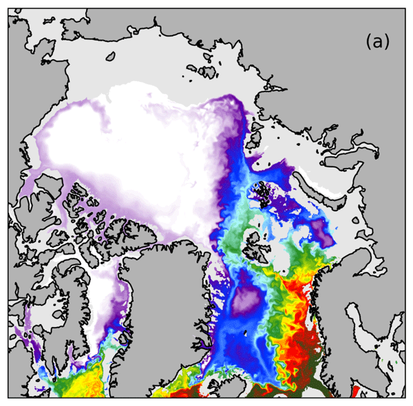
Figure 2 The first baroclinic deformation (Rossby) radius L_d [km] computed from the $\mathrm{1}/\mathrm{12}$° configuration ARCTIC12 (left), the ratio of $L_{\mathrm{d}}/min(\mathrm{d}x,\mathrm{d}y)$ for ARCTIC12 (middle) and for the $\mathrm{1}/\mathrm{4}$° configuration ARCTIC025 (right). At a ratio greater than 1.0 the model configurations has at least two grid points per L_d and starts to resolve most of the eddy field. All fields are averaged over the period 1979–2017. The white dotted line shows the 1500 m depth contour.

In this paper we examine how resolved and parameterized mesoscale eddy fluxes regulate the Atlantic Water circulation and temperature distribution in the Arctic Mediterranean, with a particular focus on the intermediate-depth Atlantic Water layer. Unlike the Southern Ocean, where eddy–mean flow interactions are relatively well understood, there is no established theoretical framework describing how mesoscale eddies shape the large-scale Arctic circulation (Timmermans and Marshall, 2020). As a result, the applicability of standard eddy parameterizations in this region, at eddy-permitting (“grey-zone”) resolution, remains uncertain. We therefore investigate how the GM parameterization modifies the time-mean circulation and tracer redistribution along the Arctic Atlantic Water pathway. We hypothesize that, in the grey-zone regime, the GM scheme primarily acts by dampening the time-mean topographically steered boundary currents through a reduction of the thermal wind-driven component of the flow, thereby modulating the large-scale flow over the Arctic Mediterranean. A central question is whether and how the eddy-induced (resolved and parameterized) redistribution of heat affects the basin-wide Atlantic Water temperature and hydrographic structure, and whether the GM formulations remains appropriate at eddy-permitting Arctic resolutions.

To study this we use two realistic pan-Arctic Ocean NEMO4-SI³ configurations, one intermediate-resolution ($\mathrm{1}/\mathrm{4}$°) configuration that is eddy-permitting and one high-resolution ($\mathrm{1}/\mathrm{12}$°) configuration that serves as a reference simulation, a “model truth”, although we note that it is not fully eddy-resolving in parts of the Arctic Ocean (see Fig. 2). The regional grids are extracted from pre-existing global grids, and most of our settings follow what is used in global models. We focus on the intermediate-resolution configuration that is in a grey zone whether the GM parameterization should be used or not. Through a set of experiments we assess the impact of the GM scheme by varying the strength of the GM diffusivity coefficient in the intermediate-resolution configuration and then compare the results with the high-resolution configuration, that is more eddy active and explicitly resolves most of the eddy fluxes, as well as to observational estimates. We diagnose the eddy energetics, eddy-induced changes to the large-scale circulation, Arctic gateway transports, hydrographic structure and Atlantic Water pathways in the Arctic Mediterranean, and eddy heat redistribution and basin heat budgets. The paper is structured as follows: in Sect. 2 we present the model configurations, experiment setup, observational data, and evaluation metrics, this is followed by the results in Sect. 3, and then we end with a summary and conclusions.

2 Methods and data

2.1 The NEMO–SI3 Arctic Ocean configurations

In our study we use two NEMO4.0.4-based (Madec et al., 2019) regional Arctic configurations covering the same geographical region and differing only in their horizontal resolution. The configurations are constructed by extracting sub-domains of already existing global configurations from the ORCA family of grids. Here we base our regional configurations on the global ORCA12 and ORCA025 grids, nominal resolutions of $\mathrm{1}/\mathrm{12}$ and $\mathrm{1}/\mathrm{4}$°, and call them ARCTIC12 and ARCTIC025, respectively. The regional domain covers the Arctic Ocean including the Nordic Seas and has two open boundaries towards the Bering Sea and North Atlantic Ocean.

The ORCA grids have a refinement of the grid size polewards and in our regional domains the horizontal resolution of ARCTIC12 (ARCTIC025) varies between 2–7 (3–20) km with domain mean resolutions of 5 (14) km. The first baroclinic Rossby radius is of O(1–15 km) in the Arctic Ocean and the Nordic Seas (see Fig. 2), which leaves ARCTIC12 in an eddy-permitting to eddy-resolving regime, and ARCTIC025 in a eddy-permitting regime. The vertical coordinate is discretised using the z^* formulation with 66 layers ranging from 5 m in the surface to 152 m at depth.

Momentum advection uses a vector-invariant formulation together with an energy and enstrophy conserving scheme, and tracer advection a Flux Corrected Transport (FCT) scheme of 4th order in both the horizontal and vertical directions. The lateral momentum diffusion uses a bi-laplacian operator applied in the horizontal directions together with a viscosity coefficient that is scaled by a defined velocity scale U_visc=0.185 and the horizontal model grid scale L as A_visc=U_viscL³ giving a domain averaged values of $-\mathrm{1.8}\times {\mathrm{10}}^{\mathrm{9}}$ and $-\mathrm{4.9}\times {\mathrm{10}}^{\mathrm{10}}$ m⁴ s⁻¹ for ARCTIC12 and ARCTIC025, respectively. The lateral tracer diffusion uses a laplacian operator applied in the isopycnal directions (Redi scheme) together with a diffusivity coefficient that is scaled by a defined velocity scale U_diff=0.0193 and L as κ_Redi=U_diffL giving a domain averaged values of 46 and 136 m² s⁻¹ for ARCTIC12 and ARCTIC025, respectively.

For the eddy-induced advection (GM scheme) we use two different formulations for the GM diffusivity coefficient κ_GM. For two of the experiments we use a standard scaling ${\mathit{\kappa }}_{\mathrm{GM}}=\frac{L_{\mathrm{d}}^{\mathrm{2}}}{T}$ based on Treguier et al. (1997) where T is the inverse baroclinic timescale and L_d the Rossby radius. For one experiment we instead use the new scaling ${\mathit{\kappa }}_{\mathrm{GM}}=\mathit{\alpha }E\frac{N}{M^{\mathrm{2}}}$ based on the GEOMETRIC scheme (Mak et al., 2018) where N is the buoyancy frequency, M² the magnitude of the lateral buoyancy gradient, E the total eddy energy, and α is the eddy efficiency parameter. The GEOMETRIC scheme solves a prognostic equation for E. The α parameter and the dissipation timescale (λ) need to be tuned to the specific application (see Mak et al., 2018), we use α=0.035 and λ=100 d.

The vertical diffusivity and viscosity are computed by a turbulent closure scheme based on the prognostic equations for the turbulent kinetic energy and its dissipation rate (Blanke and Delecluse, 1993). The background values for vertical diffusivity and viscosity are tuned down to $\mathrm{5.4}\times {\mathrm{10}}^{-\mathrm{6}}$ and $\mathrm{5.4}\times {\mathrm{10}}^{-\mathrm{7}}$ m² s⁻¹, respectively, due to the low mixing nature of the Arctic Ocean (Zhang and Steele, 2007). These background values are used to cut off the vertical mixing coefficients in the NEMO implementation of the TKE scheme to avoid numerical instabilities associated with weak mixing (Madec et al., 2019). Both the surface and bottom stresses are solved implicitly, and use a non-linear formulation with a drag coefficient of $\mathrm{1.0}\times {\mathrm{10}}^{-\mathrm{3}}$.

The model configurations are time stepped with a modified leap frog scheme including a weak Robert-Asselin filter and implicit time stepping of the vertical diffusion. Further, a time splitting approach is used to sub-step the barotropic dynamics over the main model (baroclinic) timestep. The main model timesteps (selected to satisfy the conditional stability constraint for bi-laplacian viscosity $\left|A_{\mathrm{visc}}\right|<L^{\mathrm{4}}(\mathrm{64}\mathrm{\Delta }T{)}^{-\mathrm{1}}$) are 450 and 1350 s for ARCTIC12 and ARCTIC025, respectively.

Open lateral boundary conditions for sea surface height (SSH) and barotropic velocities use the Flather radiation scheme (Flather, 1994), 3-dimensional baroclinic velocities and tracers use the Orlanski radiation scheme described in Marchesiello et al. (2001). Close to the open boundaries we define a buffer layer consisting of 8 (4) rim points for the ARCTIC12 (ARCTIC025) configuration. The total volume flux across the boundaries is balanced offline to avoid a drift in total ocean volume. At the moment no tidal components are included.

The sea ice model, SI³ (Vancoppenolle et al., 2023), discretises the ice thickness distribution using ten ice categories with an expected domain average ice thickness of 2 m. Five vertical ice layers are used for the enthalpy (temperature and salinity profile) computations. Sea ice advection uses the flux corrected 5th order Ultimate-Macho scheme, and a landfast ice parameterization (Lemieux et al., 2015) is utilized. Snow conductivity is reduced to 0.24 W(mK)⁻¹ following tuning tests of total sea ice volume and thickness in the Arctic Ocean.

2.2 Experiments

To understand how horizontal resolution and parameterized eddy fluxes impact the Atlantic Water circulation we run a set of five experiments. In one experiment we run the high-resolution configuration ARCTIC12 without GM scheme and this serves as a reference. Then we run four experiments with the intermediate-resolution configuration ARCTIC025 where we vary the κ_GM coefficients that scales the strength of the eddy-induced transport in the GM scheme. In one experiment (ARCTIC025-noGM) we run without the GM scheme. Then in two experiments we use a standard GM scaling (Treguier et al., 1997) and either scale down the computed κ_GM to 25 % of its original value (ARCTIC-lowGM) or cap the maximum value κ_GM≤2000 m² s⁻¹ (ARCTIC-highGM). Then in the last experiment we run with the GEOMETRIC scaling and use a capping value κ_GM≤2000 m² s⁻¹. The settings are summarised in Table 1, and the time-mean κ_GM fields are shown in Fig. 3. Clearly the two GM scalings differ in their spatial distributions of κ_GM. Compared to the standard scaling GEOMETRIC gives higher κ_GM in the western North Atlantic, south of Iceland, eastern Nordic Seas, and the shelf-break in Canada basin, and lower values in the eastern North Atlantic and Nansen basin. Observational estimates of surface κ_GM (Kusters et al., 2025), based on an inverse method and hydrographic data, show higher values along the western and eastern flanks of the subpolar North Atlantic and lower values in the Nordic Seas. The observational data are very patchy in the Arctic Ocean and presumably the method performs less well there. It is evident that the low κ_GM scaling is much smaller than the observations. The high κ_GM yields values that are somewhat lower in the subpolar North Atlantic, while the GEOMETRIC scaling is in line with observations in the western North Atlantic but too low in the eastern parts. In the Nordic Seas the high κ_GM scaling is quite in line with observations while the GEOMETRIC scaling yields high values. Here we compare the surface observational data to our κ_GM scalings, the observational dataset provides the 3D distribution of κ_GM that, in the North Atlantic ocean and high latitudes show a reduction in κ_GM with depth in the upper 1000 m. Our κ_GM, in contrast, lack a vertical structure. As our focus is on the impact of the GM scheme other scalings such as the lateral viscosity and diffusivity velocity scales U_visc and U_diff are kept the same between ARCTIC12 and ARCTIC025 configurations when scaling the viscosity and diffusivity (Redi) coefficients, see Table 1.

Figure 3 The time-mean (2007–2017) κ_GM fields for the (a) ARCTIC025-lowGM, (b) ARCTIC025-highGM, (c) ARCTIC025-GEOM, and d) observational estimate of surface κ_GM (Kusters et al., 2025). Note that the color range increases with increasing κ_GM.

Table 1 List of experiments used in this study with the domain average horizontal resolution, the domain average κ_Redi, and the κ_GM capping value used in the GM schemes. Note that the domain ranges are given between the brackets for horizontal resolution and κ_Redi, respectively.

All experiments also use the same atmospheric and open boundary forcings, and initial conditions. As atmospheric forcing we use 2 m air temperature, 2 m specific humidity, 10 m $u/v$ wind components, shortwave and downwelling longwave radiation, sea level pressure, total precipitation and snowfall with a 3-hourly frequency from the JRA55-do dataset (Tsujino et al., 2018). At the open boundaries we use monthly ORAS5 data (Copernicus Climate Change Service, 2021) for temperature, salinity, sea surface height, barotropic and baroclinic velocities. The experiments are started from an ocean at rest with initial conditions for salinity and temperature taken from the PHC3.0 (Polar science center Hydrographic Climatology, Steele et al., 2001) and sea ice thickness and concentration from the GLORYS12 reanalysis (European Union-Copernicus Marine Service, 2018). A monthly climatology of river runoff from the Dai and Trenberth dataset (Dai, 2017) is used. Then we run the experiments for the period 1979–2017 and do most of our analysis on the last ten years (2008–2017). The circulation timescales of Atlantic Water in the Arctic Ocean is estimated to be 15–55 years (Wefing et al., 2021) so the experiments are presumably not fully spun up. However, our main aim here is to compare the effect of the GM parameterization between different experiments with ARCTIC025 and the high-resolution ARCTIC12, so having the first 29 years as spin up should be sufficient to our purpose. In addition, we will mainly focus our analysis on the flow changes in the Nordic Seas and Eurasian¹ basin which presumably have shorter circulation timescales.

2.3 Observational data

For many of our metrics we compare the model experiments to observational estimates. Estimates of kinetic energy are taken from the dataset provided by von Appen et al. (2022). The barotropic circulation is compared to the TOPAZ4 reanalysis from the Copernicus Marine Services (ARCTIC_MULTIYEAR_PHY_002_003, 2026). Observational estimates for volume transport across the Greenland–Scotland Ridge are described in Østerhus et al. (2019) and heat transport taken from the inverse dataset provided by Tsubouchi et al. (2020). Observational estimates for Fram Strait are taken from the inverse model that combines mooring data and hydrography with GLORYS12 data (Fredriksen et al., 2025). Hydrography is compared to the PHC3.0 and WOA2018 (World Ocean Atlas 2018, Garcia et al., 2019) climatological datasets, and the GLORYS12 and SODA4 (Simple Ocean Data Assimilation version 4, Chepurin et al., 2025) reanalysis products. The observational estimates for κ_GM are from the dataset provided by Kusters et al. (2025).

2.4 Model evaluation metrics

To evaluate the model simulations we compute a number of metrics that are briefly described below. To analyse the impact on energetics we compute the total kinetic energy which can be partitioned into mean kinetic energy (MKE) and eddy kinetic energy (EKE) using Reynolds decomposition,

$$\begin{array}{}\text{(3)}& \mathrm{EKE}={\displaystyle \frac{\mathrm{1}}{\mathrm{2}}}\left(\overline{u^{\mathrm{2}}}+\overline{v^{\mathrm{2}}}\right)-{\displaystyle \frac{\mathrm{1}}{\mathrm{2}}}\left({\overline{u}}^{\mathrm{2}}+{\overline{v}}^{\mathrm{2}}\right),\end{array}$$

where u and v are the horizontal velocity components in zonal and meridional directions, and overline denotes the temporal (monthly) average. Note that with this decomposition the EKE contains energy contributions from all variations on time-scales shorter than 1 month, not only that contained by the coherent eddies.

To analyse the large-scale circulation we compute the barotropic streamfunction by integrating the barotropic meridional transport in the zonal direction,

$$\begin{array}{}\text{(4)}& \begin{array}{rl}{\mathit{\psi }}_{\mathrm{bt}}(x,y,t)& =\underset{x_{\mathrm{east}}}{\overset{x}{\int }}\underset{-H}{\overset{\mathit{\eta }}{\int }}v(x^{\prime },y,z,t)\mathrm{d}z\mathrm{d}{x}^{\prime }\\ & =\underset{x_{\mathrm{east}}}{\overset{x}{\int }}V(x^{\prime },y,t)\mathrm{d}{x}^{\prime },\end{array}\end{array}$$

where $v(x,y,z,t)$ is the meridional velocity component and H the depth. To further assess the dominant driver of gyre dynamics we can consider the depth integrated meridional volume transport equation,

$$\begin{array}{}\text{(5)}& fV=-H{\displaystyle \frac{\partial P_{\mathrm{b}}}{\partial x}}+{\displaystyle \frac{\partial \mathrm{\Phi }}{\partial x}}-{\displaystyle \frac{{\mathit{\tau }}_x}{{\mathit{\rho }}_{\mathrm{0}}}},\end{array}$$

where f is the Coriolis parameter, H the local depth, P_b is the bottom pressure, and τ_x the wind stress along the zonal direction (Born et al., 2009; Wang et al., 2020).

$$\begin{array}{}\text{(6)}& \mathrm{\Phi }=g\underset{-H}{\overset{\mathrm{0}}{\int }}{\displaystyle \frac{{\mathit{\rho }}_{\mathrm{ref}}-\mathit{\rho }}{{\mathit{\rho }}_{\mathrm{ref}}}}z\mathrm{d}z\end{array}$$

is the potential energy term computed from the vertically integrated depth-weighted density anomaly with ρ_ref a reference density for sea water. In Eq. (6), $\partial \mathrm{\Phi }/\partial x$ represents the depth-integrated thermal wind contribution to the transport and is therefore sensitive to changes in density stratification associated with both parameterized and resolved eddies. Other contributions are not discussed further: the wind-stress term is similar among the experiments, and the bottom pressure term cannot lead to flow amplification (Born et al., 2009).

Because of the depth weighting by z, the potential energy term is particularly sensitive to density changes in the deep water. We therefore adopt a slightly modified form of Eq. (6):

$$\begin{array}{}\text{(7)}& \mathrm{\Psi }={\displaystyle \frac{g}{f}}\underset{-h_{\mathrm{b}}}{\overset{\mathrm{0}}{\int }}\mathrm{\Delta }{\mathit{\rho }}^{*}z\mathrm{d}z\end{array}$$

where

$$\begin{array}{}\text{(8)}& \mathrm{\Delta }{\mathit{\rho }}^{*}=\left[\mathit{\rho }\right(T_{\mathrm{DW}},S_{\mathrm{DW}},z)-\mathit{\rho }(T,S,z\left)\right]/\mathit{\rho }(T_{\mathrm{DW}},S_{\mathrm{DW}},\mathrm{0})\end{array}$$

denotes the density anomaly of the Atlantic Water layer relative to the deep water with reference values $T_{\mathrm{DW}}=-\mathrm{1}$ °C and S_DW=34.9 g(kg)⁻¹ (Broomé et al., 2020); $\mathit{\rho }(T,S,z)$ is the local density with depth used as a proxy for pressure. The inflowing Atlantic Water in the Arctic Mediterranean typically occupies the upper 800–1000 m, mainly limited by the sill depth at Greenland–Scotland Ridge. Here we choose the integration limit h_b=854 m that represent by a fixed model level that is close to the real sill depth at Greenland–Scotland Ridge. In the following, we refer to Ψ as the baroclinic transport function.

Another scalar metric that we use to assess the large scale circulation is the topostrophy (Holloway, 2008)

$$\begin{array}{}\text{(9)}& \mathcal{T}=\text{sgn}\left[f\right](\widehat{\mathit{z}}\cdot \mathit{u}\times \mathrm{\nabla }H).\end{array}$$

Topostrophy measures the alignment of a flow with the isobaths where a positive topostrophy represents a prograde flow, i.e., with shallower water to the right of the flow direction. Note that the large scale bathymetric slope in the Arctic Ocean yields a prograde flow that is mostly a large scale cyclonic circulation. Although locally a retrograde slope can still be part of a larger cyclonic circulation (e.g. Kallmyr et al., 2025).

Further, we also compute the volume and heat transport across a number of key sections. The volume transport across a section is computed as

$$\begin{array}{}\text{(10)}& F=\underset{A}{\iint }{v}_{⟂}(x,z)\mathrm{d}A\end{array}$$

where v_⟂ is the cross-sectional velocity, A the cross-sectional area. The heat transport is computed as

$$\begin{array}{}\text{(11)}& Q=c_p{\mathit{\rho }}_{\mathrm{0}}\underset{A}{\iint }\mathit{\theta }\left(v_{⟂}\right(x,z)-\stackrel{\mathrm{‾}}{v})\mathrm{d}A\end{array}$$

where θ is the potential temperature, c_p=3992 J K⁻¹ kg⁻¹ the specific heat, and ρ₀=1026 kg m⁻³ a reference density of seawater. $\stackrel{\mathrm{‾}}{v}$ is the mean velocity computed across all cross sections enclosing the Nordic Seas to assure a closed volume budget across the sections (Schauer and Beszczynska-Möller, 2009).

Finally, we compute the horizontally averaged heat trend terms for the model. The heat trend term in NEMO can be expressed as,

$$\begin{array}{}\text{(12)}& c_p{\mathit{\rho }}_{\mathrm{0}}{\displaystyle \frac{\partial \mathit{\theta }}{\partial t}}=-\mathrm{\nabla }\cdot (c_p{\mathit{\rho }}_{\mathrm{0}}\mathit{u}\mathit{\theta }+{\mathbf{F}}_{\mathrm{sgs}})+F_{\mathrm{surf}}\end{array}$$

where F_surf is the surface heat flux, and F_sgs represents subgrid scale parameterizations which includes contribution from penetrative shortwave radiation, convection, bottom boundary layer parameterization, vertical diffusion, convection, isopycnal (Redi) diffusion, and Asselin time filter. Each term in Eq. (12) is diagnosed online in the model. To obtain a closed budget, each term is additionally multiplied by the time-varying cell thickness dz at every time step, since the layer thickness evolves in the z^* coordinate formulation. Then we integrated horizontally for each model layer and scale by the layer volume to get profiles of horizontally averaged heat trend terms. Following Eq. (1) the heat advection term in Eq. (12) can then be further decomposed into mean, resolved and parameterized eddy contributions. For a more detailed description of how to diagnose and decompose heat trends see, e.g., Griffies et al. (2015).

3 Results

To understand how both horizontal resolution and GM scheme impact the circulation and hydrography we now look at a number of different metrics. First we analyze the impact on model energetics by investigating the kinetic energy partitioning. This is followed by an analysis of the large-scale circulation and the Arctic gateways transport. Finally, we look at the impact on the hydrographic structure and heat redistribution.

3.1 Partitioning of mean and eddy kinetic energy

First we focus on total kinetic energy of the Atlantic Water layer to see how energetic and eddy active the model configurations are, since this has implications for the redistribution of salt and heat as well as the strength of the boundary current. In Fig. 4 the time-mean partitioning of total kinetic energy into MKE and EKE in the Atlantic Water layer (at 233 m depth) is shown. It is evident that both the resolution and the GM scheme impact the MKE as the ARCTIC12 and ARCTIC025-noGM have much higher levels in the Nordic Seas and central Arctic Ocean. The levels are high not only in the boundary current, but also in the basin interiors. The EKE, on the other hand, is generally low in the models, except for the ARCTIC12 that has elevated levels of EKE in the central Norwegian Sea which are about one order of magnitude greater than ARCTIC025 configurations. All configurations show slightly higher levels of EKE along the boundary current pathway and in the Fram Strait region, and lower levels in the interior. This is to some extent in agreement with the observations (Fig. 4k) although the levels are higher in the observations.

Figure 4 Panels (a)–(e) show the time-mean (2008–2017) MKE and panels (f)–(j) the EKE in the Atlantic Water layer (233 m depth) for the ARCTIC12, ARCTIC025-noGM, ARCTIC025-lowGM, ARCTIC025-highGM, and ARCTIC025-GEOM, respectively. Panel (k) shows observations of EKE from von Appen et al. (2022), averaged over the depth range 500–1000 m, with the grey line showing the 233 m isobath. Panels (l) and (m) show spatial averages of MKE and EKE at selected regions (green boxes in f) along the Atlantic Water pathway. The regions are NS = Norwegian Sea, WSC = West Spitzbergen Current, WNB = Western Nansen Basin, and ENB = Eastern Nansen Basin.

To demonstrate the difference in MKE and EKE we compute the spatial averages at four selected regions along the boundary current. Figure 4 shows that the MKE of the boundary current is generally higher in the high-resolution simulation (ARCTIC12) and is reduced with the GM scheme where ARCTIC025-highGM/ARCTIC025-GEOM (which has the strongest eddy-induced transport) have lower levels. In all experiments the MKE in the boundary current also drops to lower levels when entering the western Nansen basin. Then in the eastern Nansen basin it increase to even higher levels than in the Norwegian Sea and West Spitzbergen Current. This is presumably due to a more energetic Barents Sea branch that connects to boundary current just upstream at St. Anna Trough.

Figure 4 also shows that the partitioning of total kinetic energy is different between the high-resolution and intermediate-resolution experiments in the Norwegian Sea region. Here EKE constitutes 41 % and 18 %–12 % of total kinetic energy in the ARCTIC12 and ARCTIC025s, respectively. Inside the Arctic Ocean (regions WNB and ENB) the contribution of EKE drops off in the high-resolution experiment. Here EKE is only 16 % of the total kinetic energy in ARCTIC12 and 5 %–12 % in the intermediate-resolution experiments. We note that the high-resolution simulation exhibits an EKE distribution in the Nansen Basin that is qualitatively consistent with the very high–resolution (1 km) model study of Müller et al. (2024), but with systematically lower EKE levels. This likely reflects the fact that our simulation is not fully eddy-resolving in this region (see Fig. 2). The lower values in the spatial averages partly also reflects the gradient in EKE in the basin interior which is seen both in observations and model simulations (Fig. 4f–k). The GM scheme also reduces the EKE in the boundary current regions. The drop off in eddy activity between the experiments and the dampening effect of the GM scheme on the resolved eddy field can also be clearly detected in snapshots of relative vorticity and potential temperature (Figs. A1 and A2).

3.2 Eddy-induced modification of the large-scale circulation

3.2.1 Barotropic circulation and the Greenland Sea Gyre

Next, we focus on the large-scale barotropic circulation. Figure 5 shows the time-mean barotropic circulation in the different experiments as well as the Arctic reanalysis TOPAZ4 (from the Copernicus Marine Services, ARCTIC_MULTIYEAR_PHY_002_003, 2026). All experiments show a cyclonic circulation over the northern North Atlantic, Nordic Seas and Eurasian basin. Over the Canada basin there is mostly an anticyclonic circulation in all experiments except ARCTIC025-noGM. A similar circulation pattern with cyclonic/anticyclonic circulation is seen in TOPAZ4 as well. ARCTIC025-noGM instead has a weak cyclonic circulation over the Canada basin. The observed upper ocean circulation in the Canada basin tend to be mostly anticyclonic while the circulation in the Atlantic Water layer is cyclonic (e.g. Rudels et al., 2011). The upper ocean circulation of Polar Surface Water is dominantly anticyclonic over the Canada basin in all experiments (not shown). This suggests that excluding the GM parameterization leads to a too strong mean Atlantic Water layer circulation in the intermediate-resolution configuration which then dominates the contribution to the vertically integrated barotropic circulation in the Canada basin.

Figure 5 Panels (a)–(e) show the time-mean (2008–2017) barotropic streamfunction [Sv] for the ARCTIC12, ARCTIC025-noGM, ARCTIC025-lowGM, ARCTIC025-highGM, and ARCTIC025-GEOM, respectively. Panel (f) shows the barotropic streamfunction for the TOPAZ4 reanalysis averaged over the same period, and (g) show the yearly mean temporal evolution of the spatial averaged barotropic streamfunction. The Greenland Sea Gyre spatial averaging is done over the purple box shown in (a)–(f), and the white lines show the −45 Sv isoline in the subpolar gyre.

The circulation over the Nordic Seas is dominated by the Greenland Sea Gyre which is stronger in the ARCTIC025-noGM/lowGM than the ARCTIC12 and ARCTIC025-highGM/ARCTIC025-GEOM configurations. Clearly the strength of the barotropic circulation is impacted by the GM scheme and the strength of the eddy-induced transport. This is further seen in Fig. 5g that shows the strength of the Greenland Sea Gyre with time. As the model starts to adjust to the forcing the response is different between the different configurations. ARCTIC12 and ARCTIC025-highGM adjust to a similar gyre strength (−8.9 Sv for the period 2008–2017), while the ARCTIC025-GEOM strength is 1.5 Sv weaker and the ARCTIC025-noGM/ARCTIC025-lowGM is 2 Sv stronger. This is stronger than the gyre strength in the TOPAZ4 (−5.9 Sv), but in line with the −8 to −10 Sv range from the multi model study by Muilwijk et al. (2019). However, we note that both TOPAZ4 and most of the models in Muilwijk et al. (2019) use different atmospheric forcing than our experiments which might impact the strength of the gyre.

It is also seen in Fig. 5 that the subpolar gyre is stronger in the high-resolution simulation. For the time-mean barotropic streamfunction the minimum is −67 Sv in ARCTIC12 and −51, −54, −53, and −49 Sv in ARCTIC025-noGM, ARCTIC025-lowGM, ARCTIC025-highGM, and ARCTIC025-GEOM, respectively. TOPAZ4, in contrast, has a much weaker subpolar gyre with a minimum of −28 Sv. A similar increase in the subpolar gyre strength with resolution has also been reported by Hirschi et al. (2020) where they compare eddy-rich simulations to coarse resolution simulations. However, since the open boundary is very close to the southern extent of the subpolar gyre the results should be interpreted with caution.

3.2.2 Changes in the topographically steered Atlantic Water boundary current

In contrast to the tropical and sub-tropical oceans where the wind-stress curl is balanced by depth-integrated meridional transport (Sverdrup balance), the Sverdrup balance does not hold in the Arctic Mediterranean due to the influence of topography and the β-effect being negligible at high latitudes (β is here the meridional gradient of the Coriolis parameter) (Timmermans and Marshall, 2020). Instead of being constrained by the β-effect the potential vorticity-conserving barotropic flow is controlled by bottom topography and wind-stress integrated along closed $q=f/H$ contours (Nøst and Isachsen, 2003; Timmermans and Marshall, 2020). Integrating wind stress along closed $f/H$ contours around the whole Arctic Mediterranean yield mostly positive values indicating that the linear model by Nøst and Isachsen (2003) yields a barotropic flow that is dominantly cyclonic, with the Icelandic low being the main driver (Timmermans and Marshall, 2020). The flow aligns with constant q contours which in the high latitude essentially coincide with isobaths due to f being nearly constant. From topostrophy (Eq. 9) we can estimate the change in the along-isobath flow in our simulations.

In Fig. 6a–e it is seen that the barotropic flow has a dominantly positive topostrophy along the circum-Arctic Atlantic Water pathway in all simulations, showing that they maintain a cyclonic large-scale flow and supports earlier theoretical and observational studies (e.g. Nøst and Isachsen, 2003; Aaboe and Nøst, 2008; Aaboe et al., 2009; Kallmyr et al., 2025; Sjur et al., 2025). This is in contrast to some early Arctic models which had problems simulating the large-scale Atlantic Water flow and sometimes showed negative topostrophy, see model intercomparison in Holloway et al. (2007). From Fig. 6f–g it is clear that the GM scheme mostly reduces the topostrophy along the Norwegian Sea and Eurasian basin thus damping the along isobath flow. To further assess the impact on the baroclinic component of the along isobath flow we show the topostrophy of the full flow in Fig. 6i–m. Here it is seen that the ARCTIC025-noGM experiment has a much stronger baroclinic component, with steeper gradients in density towards the shelf and strong thermal wind shear with a flow reversal with depth. Introducing the GM scheme flattens the isopycnals and leads to a barotropization of the flow. Compared to ARCTIC025, simulations ARCTIC12 has a much more barotropic structure, and the flattening of isopycnals and spread of the warm and salty Atlantic Water core further into the basin indicate eddy–mean interactions between the boundary current and the interior. Overall we see that the GM scheme damps topographically steered barotropic circulation, leading to weaker boundary currents and reduced alignment with bathymetry.

Figure 6 Panels (a)–(e) show topostrophy of the barotropic flow for the different experiments, and (f)–(h) the difference in topostrophy between the ARCTIC025-lowGM, ARCTIC025-highGM and ARCTIC025-GEOM relative to ARCTIC025-noGM; blue means a decrease relative to ARCTIC025-noGM.

The main mechanism through which resolved and parameterized eddies can impact the large-scale barotropic flow is through a reduction of the thermal wind-driven component (in Eq. 5). To complement the analysis of topostrophy we here show the baroclinic transport function which represents the part of the circulation driven by density gradients and stratification. Figure 7a–c show that the ARCTIC025-noGM experiment has a much stronger baroclinic transport (higher values and steeper gradient of Ψ) along the Atlantic Water pathway compared to ARCTIC12. This may be understood as the poorly resolved eddy buoyancy fluxes in ARCTIC025 cannot release the stored available potential energy in the boundary current promoting an excessively strong baroclinic component of the flow. As the GM scheme is introduced in the ARCTIC025 experiments the strength of the baroclinic transport reduces along the most of the Atlantic Water pathway (Fig. 7d–f). This can be interpreted from the decrease in available potential energy where it is high (in the boundary current) and increase in regions where it is low. However, in the Norwegian Sea where the EKE is relatively high in then ARCTIC025-noGM (Fig. 4) the response is mixed with some regions showing an increase in available potential energy along the boundary current pathway suggesting a stronger buoyancy redistribution locally by the resolved eddy field in ARCTIC025-noGM than the GM scheme.

Figure 7 Panels (a) and (b) show the baroclinic transport function in ARCTIC12 and ARCTIC025-noGM, respectively. Panel (c) shows the difference between ARCTIC025-noGM and ARCTIC12. Panels (d)–(f) differences ARCTIC025-lowGM, ARCTIC025-highGM and ARCTIC025-GEOM relative to ARCTIC025-noGM. Note that regions shallower than the integration depth of 854 m has been masked out.

3.3 Arctic gateway transports

3.3.1 Volume and heat transport across the Greenland–Scotland Ridge

The Greenland–Scotland Ridge forms the main oceanic gateway connecting the North Atlantic and the Arctic Mediterranean, and the transports across the ridge therefore reflect the upstream conditions for inflowing Atlantic Water to the Nordic Seas. The volume and heat transports across the Greenland–Scotland Ridge are computed by integrating Eq. (10) over different density intervals using potential density anomalies ${\mathit{\sigma }}_{\mathrm{0}}=\mathit{\rho }-\mathrm{1000}$, where ρ is the potential density referenced to surface pressure. Here we distinguish between inflow and overflow water masses using 27.8 kg m⁻³ as the limit at Iceland–Faroe and Denmark Strait gateways and 27.65 kg m⁻³ at Faroe–Scotland. For the Denmark Strait we further sub-divide the lower density range using 27.45 kg m⁻³ to include the outflow water masses that constitutes the buoyant water exported by the East Greenland Current. To close the northward transport to the Nordic Seas we also include the net inflow at Scotland–Norway gateway.

Table 2 Time-mean (2008–2017) volume transport [Sv] across the Greenland–Scotland Ridge which constitutes the Denmark Strait, Iceland–Faroe, and Faroe–Scotland gateways. The transports are divided into inflow and overflow components computed based on density limits. Note that the Denmark Strait gateway also has an additional outflow component that includes less dense water returning southward in the East Greenland Current. We also show the transport across the Scotland–Norway gateway that only has an inflow component. See Fig. 1 for the location of the gateways. The Observational estimates are from Østerhus et al. (2019).

The time-mean volume transport across Greenland–Scotland Ridge is shown in Fig. 8 as well as the summed total inflow, overflow and outflows in Table 2. From Table 2 it is seen that the inflow of Atlantic Water towards the Nordic Seas across Greenland–Scotland Ridge is quite in line with observations for the ARCTIC12, ARCTIC025-noGM and ARCTIC025-lowGM experiments, while ARCTIC025-highGM and ARCTIC025-GEOM experiments have a weaker inflow. The partitioning of the inflow between the different gateways is also different between experiments. At Iceland–Faroe gateway almost all experiments are consistent with observations except ARCTIC025-GEOM which has a much lower transport. The density of the peak inflow varies between the experiments, with ARCTIC12 and ARCTIC025-highGM shifted towards slightly lower densities (Fig. 8a). At the Faroe–Scotland gateway the inflow in ARCTIC12, ARCTIC025-noGM, ARCTIC025-lowGM, ARCTIC025-GEOM are stronger and ARCTIC025-highGM in line with observations. At Denmark Strait both the inflows and outflows are slightly stronger in ARCTIC12 and ARCTIC025-GEOM compared to the other experiments, but weaker than observations. However, as seen in Fig. 8 the shift from a net inflow to outflow is not well-defined with a fixed density limit, so the results should be interpreted with caution. We also note that all experiments have a much weaker inflow at the Scotland–Norway gateway compared with observations. However, the observational estimates from Østerhus et al. (2019) includes the contribution of the inflow on the Scottish shelf (they estimated it to be 0.4–0.5 Sv). In our analysis we have chosen a closed section between Faroe Islands and Scotland instead of only covering the Faroe Bank Channel because it simplifies transport calculations and comparisons between grids of different resolutions. This leads to an offset with higher (lower) values in our Faroe–Scotland (Scotland–Norway) gateway in our analysis compared to observations.

Figure 8 Time-mean (2008–2017) volume transport across the Greenland–Scotland Ridge, here binned into density classes for the separate gateways Iceland–Faroe (a), Faroe–Scotland (b), and Denmark Strait (c). The thin dash and dotted lines show in- and outflow, respectively; and the solid line the netflow. The dash black horizontal lines show limiting densities for computing inflows and overflows (and outflows for Denmarks Strait).

Also the overflow across the Greenland–Scotland Ridge is weaker in all experiments compared to the observational estimate. Here the high-resolution experiment stands out with a stronger overflow compared to the intermediate-resolution counterparts, possibly due to better resolving the channels of the gateways. Especially in the Denmark Strait the overflow seems to be much weaker in the intermediate-resolution experiments. For ARCTIC025 experiments the peak overflow density is slightly lower than ARCTIC12 (Fig. 8c). For the Greenland–Scotland Ridge overflow there is no impact of the GM scheme on the ARCTIC025-highGM. Mayer et al. (2023) compares the Greenland–Scotland Ridge transport in five different reanalysis products and two hindcasts and find that the Atlantic Water inflow ranges between 6.8 to 8.3 Sv and the overflow between −4.4 to −5.4 Sv, our experiments are in the range of 7.1 to 7.7 and −4.1 to −4.7 Sv, respectively.

The net northward heat transport that Atlantic Water carries across the Greenland–Scotland Ridge is computed using a closed volume budget across the Nordic Seas (Eq. 11). Here we only report the transports at the three main gateways (Iceland–Faroe, Faroe–Scotland and Denmark Strait) that are presented in Table 3. The total northward heat transport in the in ARCTIC12, ARCTIC025-noGM, ARCTIC025-lowGM and ARCTIC025-GEOM are similar while ARCTIC025-highGM is lower. The magnitude of heat transport in the two main gateways Iceland–Faroe and Faroe–Scotland are consistent with the northward volume transports (Table 2). Our experiments are well in line 266 to 280 TW with the observational estimates of 277 TW (Tsubouchi et al., 2020), but somewhat higher than the reanalysis products (219 to 265 TW) reported by Mayer et al. (2023).

Overall, the simulations reproduce the observed magnitude of Atlantic Water inflow across the Greenland–Scotland Ridge reasonably well, although differences remain in the partitioning between gateways and in the representation of overflow transports. Experiments with weaker or no eddy-induced transport exhibit stronger Atlantic Water inflow while stronger parameterized eddy mixing reduces it. For the standard scaling, that has a more uniform κ_GM (Fig. 3) field south of Greenland–Scotland Ridge, increasing its strength shifts the partitioning between Iceland–Faroe and Faroe–Scotland branches to the former being stronger, and more in line with observations. The GEOMETRIC scaling has a more heterogeneous κ_GM south of Greenland–Scotland Ridge with locally high values south of Iceland presumably leading to a weaker Iceland–Faroe branch. Locally at the strait (not shown) there is a reduction in the baroclinic structure compared to the ARCTIC-noGM.

Table 3 Time-mean (2008–2017) net northward heat transport [TW] across Greenland–Scotland Ridge. See Fig. 1 for the location of the gateways. The observational estimates are from Tsubouchi et al. (2020).

3.3.2 Volume and heat transport across the Barents Sea Opening and Fram Strait

Next we consider the exchange between the Nordic Seas and the Arctic Ocean by looking at the time-mean volume and heat transports across the Barents Sea Opening and Fram Strait (Table 4). Note that here we compute the transport over the whole water column rather than separating it into different density classes as we did for Greenland–Scotland Ridge. It is seen that the net volume transport across Barents Sea Opening is slightly stronger in the high-resolution experiment than in the intermediate-resolution experiments. The in- and outflows, however, are much stronger (more than 1 Sv higher in each direction) in the high-resolution experiment. Table 4 also shows that the effect of the GM parameterization is quite modest on the volume transport across Barents Sea Opening, however, ARCTIC025-GEOM has somewhat higher transport than the other ARCTIC025 experiments. Compared to observations, all model experiments exhibit a higher net volume transport than the 2.0 Sv estimated by Smedsrud et al. (2010), but a lower transport than the 3.6 Sv inverse-model estimate of Tsubouchi et al. (2012), even though the simulated in- and outflows exceed those reported by Tsubouchi et al. (2012). The net northward heat transport follows the patterns of volume transport with the high-resolution experiment somewhat stronger than the intermediate-resolution experiments, and that all model experiments have slightly lower heat flux than the inverse model estimate by Tsubouchi et al. (2012). Our experiments show an increase in both the net volume and northward heat transport across Barents Sea Opening with time (not shown), which is also consistent with model simulations by Muilwijk et al. (2018).

Table 4 Time-mean (2008–2017) volume [Sv] and heat [TW] transport across the Barents Sea Opening and Fram Strait. A positive volume transport means a northward flow towards the Arctic Ocean. For the heat transport we only report the northward “in” component. See Fig. 1 for the location of the gateways.

^a Smedsrud et al. (2010), ^b Tsubouchi et al. (2012), ^c Schauer et al. (2008), ^d Rudels et al. (2015)

In the Fram Strait (Table 4) the net volume transport is dominated by a southward flow in all experiments. Here the high-resolution experiment have a much stronger net, and in- and outflows compared to the intermediate-resolution experiments. The intermediate-resolution experiments further show that, in contrast to the Barents Sea Opening, the volume transport at Fram Strait is impacted by the GM parameterization. Here the experiments with a strong eddy-induced transport have a stronger net southward transport. The main reason is that the inflows are reduced more than the outflows. This is in agreement with the local reduction (increase) of the barotropic flows topostrophy locally in the western (eastern) flanks of Fram Strait relative ARCTIC025-noGM shown in Fig. 6f–h, and a reduction of baroclinic transport in the upper 1000 m on particularly the eastern flank (Fig. 7d–e). Since the net inflows through Barents Sea Opening and Bering Strait (not shown) are small between the experiments, a consequence of this asymmetric local response is that the GM scheme changes the partitioning of the net southward flow on eastern and western sides of Greenland. Without the GM scheme the net southward flow at Fram Strait is too weak compared to observations and the high-resolution experiment, and by volume conservation, too high through the western side of Greenland (Canadian Arctic Archipelago and Nares Strait). We also note that for the experiments with strong eddy-induced transport the GEOMETRIC scheme gives a stronger southward flow than the standard GM formulation. Another consequence of the reduction in flow strength by the GM scheme is a reduced net heat transport into the Arctic Ocean (Table 4). This follows since the heat input through Fram Strait is mainly controlled by the inflow branch (e.g. Rudels et al., 2015).

3.4 Hydrographic structure and Atlantic Water pathways

3.4.1 Hydrographic and velocity structure at the Fram Strait

The Fram Strait is the deepest gateway to the Arctic Ocean and an important pathway for the water mass exchange between the Arctic Ocean and North Atlantic Ocean. To further see the impact of the resolution and the GM parameterization on the circulation and water mass exchange we show the potential temperature, salinity, density and cross-sectional current speed in Fig. 9. We focus on the water masses and flow of the upper 1000 m. Here the flow is expected to be dominated by northward flowing Atlantic Water in the West Spitzbergen Current on the eastern flank of the strait and recirculating Atlantic Water situated more centrally in the strait. On the western flank we expect southward flowing Polar Surface Water in East Greenland Current, and returning Atlantic Water below the East Greenland Current, that has been cooled slightly on its path circulating around the Arctic Ocean (e.g. Beszczynska-Möller et al., 2012).

Figure 9 Time-mean (2008–2017) Fram Strait (78° N) potential temperature, density and salinity (a–f), and cross-sectional current (g–l) for the different experiments as well as observational estimates based on an inverse model.

The potential temperature and cross-sectional current structures in the experiments (Fig. 9) reveal a core of warm (T>3 °C) Atlantic Water in the West Spitzbergen Current. Compared to the observational estimate (Fig. 9f) the ARCTIC025 experiments all have warmer water centrally in the strait. In the upper western part of the strait there is a well-defined cold (T<0 °C) water mass of Polar Surface Water, somewhat shallower than the observational estimate. Below the Polar Surface Water there is also returning Atlantic Water with slightly warmer ($\mathrm{0}<T<\mathrm{3}$ °C) temperatures. Also here the ARCTIC025 experiments are somewhat warmer. A similar pattern holds for salinity, where the salinities are higher in the inflow region and outflowing Atlantic Water region. This impacts the density distribution across the strait, and therefore the baroclinic currents. Overall it is the salinity gradients that control the density structure. On the eastern side of the strait, in the West Spitzbergen Current, ARCTIC025 has slightly flatter slopes compared to ARCTIC12, while on the western side the density structure below the Polar Surface Water differ significantly between ARCTIC12 and ARCTIC025 experiments. In ARCTIC12 the isopycnals slope downwards towards Greenland, while they slope upwards in ARCTIC025 experiments due to the higher salinities. On both sides the flattening effect of GM is evident, however it is most pronounced on the eastern side where isopycnals (and isohalines) are steeper. The weaker thermal wind shear on both sides of the strait also leads to weaker cross-sectional currents (Fig. 9g–l) in the ARCTIC025 experiments compared to ARCTIC12 and the observational estimate. We also note that the outer offshore West Spitzbergen Current branch centred around longitude 0–5° E in the observational estimates is not present in the model simulation at 78° N, however, further north the simulated currents splits up into two branches (not shown). This is presumably due to the bathymetric representation in the model configurations.

3.4.2 Atlantic Water layer temperature distribution

Observations show that in the Nordic Seas the warmest temperatures are found close to the surface while in the Arctic Ocean the core of the Atlantic Water layer is situated somewhere between 100–800 m. The depth of the Atlantic Water layer core typically deepens from 250 m in the Nansen basin to 300–400 m in the Amundsen, Makarov and Canada basins (e.g. Timmermans and Marshall, 2020). Here we select the model level corresponding to 233 m, which thus mainly represents the Atlantic Water layer core temperature in the Nansen basin. Selecting deeper levels in the model show qualitatively similar results. To assess the simulated temperature in the Atlantic Water layer we compare our experiments with two climatologies (PHC3.0 and WOA2018) and two reanalysis products (GLORYS12 and SODA4). We select these comparison datasets to illustrate: (i) the warming between the older PHC3.0 and newer WOA2018 climatologies in the Nordic Seas and Arctic Ocean (Fig. 10f, g); (ii) the difficulty of representing the Atlantic Water circulation in state-of-the-art reanalyses, with GLORYS12 exhibiting an overly cold eastern Nansen Basin compared to SODA4 (Fig. 10h, i). Note that both reanalyses are of similar resolution to our ARCTIC12 experiment.

Figure 10 shows the time-mean Atlantic Water layer potential temperature from the model simulations. It is seen that, in the Norwegian and Greenland seas, the GM scheme leads to generally warmer average temperatures, and that the ARCTIC12 is slightly warmer (colder) than the warmest ARCTIC025 experiments in the Norwegian Sea (Greenland Sea), respectively. In the Nansen basin, the average temperatures essentially follows the net heat exchange in the Fram Strait (Table 4) with the ARCTIC025-highGM significantly colder (and with lower heat input) than the other experiments. In the Amundsen basin, the ARCTIC025-noGM experiment, which has the strongest boundary current, is comparatively warmer than the other experiments. We caution that, compared to the other sub-regions, the Amundsen basin takes longer to spin-up which might impact the results in our analysis.

Next we compare the simulated temperatures to the climatologies and reanalysis. In the Norwegian Sea the spread in the comparison products is 4.3–5.0 °C. This can be compared with the spread in the simulations of 4.6–5.2 °C. In the Greenland Sea all the comparison products show a narrower range (0.6–1.0 °C) and suggest that the simulations are biased towards too high average temperatures (1.7–2.2 °C). In the Nansen basin the comparison products and experiments show similar ranges of 1.2–1.7 and 1.2–1.9 °C, respectively. For the Amundsen basin the comparison products are generally warmer than the simulations. For the comparison products, the PHC3.0 is always the coldest and mainly represents conditions from the 1970s to 2000s, and since recent studies suggest a warming of the Arctic Ocean (Polyakov et al., 2023; Smedsrud et al., 2022), we place more trust in the warmer end of the given temperature ranges above.

Figure 10 Time-mean (2008–2017) potential temperature in the Atlantic Water layer (233 m depth) for the different experiments; PHC3.0 and WOA2018 climatologies; and GLORYS12 and SODA4 reanalysis. The inset numbers in the lower left part of each sub-panel are horizontally averaged temperatures for the regions shown in sub-panel (a). From top to bottom the numbers represent: Norwegian Sea, Greenland Sea, Nansen basin, and Amundsen basin. Also see Fig. 1 for the name and location of the different sub-basins.

3.5 Eddy heat redistribution and basin heat budgets

3.5.1 Eddy heat flux divergence

In Fig. 10 it is seen that the lateral spread of heat is different in some parts of the domain. In the northern Norwegian Sea and Nansen basin the GM scheme seem to impact the width of the warm region close to the boundary current, and in the central Greenland Sea the temperature gradient between the warm boundary current and cold interior is eroded. To further analyse this we computed the divergence of eddy temperature flux. Figure 11 shows the horizontal component of the divergence of both the resolved and parameterized (GM) eddy temperature flux. From the resolved eddy temperature flux divergences it is evident that the ARCTIC025 lack much of the heating and cooling from eddies in the central parts of the Norwegian Sea that is seen in ARCTIC12, and that the Greenland Sea and Nansen basin have very weak eddy contributions beyond the weak signal close to the boundary currents. The signal in ARCTIC12 is rather noisy in the Norwegian Sea, similar to the surface signal analysed by Isachsen et al. (2012). There is also evidence of cooling in the core of the boundary current and heating immediately adjacent to it. Similar, and less noisy features, are seen in the ARCTIC025 experiments, which are progressively reduced with increasing GM strength. The parameterized eddy temperature flux divergences, on the other side, show similar but much stronger and coherent signals of heating and cooling along the boundary current and the interior regions. Here the parameterized GM fluxes contribute significantly to the lateral redistribution of heat in the northern Norwegian Sea, central Greenland Sea, and in regions adjacent to the boundary current in the Nansen basin. Both the resolved and parameterized eddy temperature flux divergences also have a significant vertical component (not shown) that tend to cool the core of the boundary current and heat immediately adjacent to it at this depth.

Figure 11 Horizontal component of the time-mean (2008–2017) divergence of resolved and parameterized eddy temperature fluxes in the Atlantic Water layer (233 m depth) for the different experiments.

3.5.2 Horizontally integrated heat budgets and eddy contributions

Finally, we compare the contributions of parameterized and resolved eddy temperature fluxes to other components of the simulated temperature trend given in Eq. (12) by horizontally averaging each term over the Norwegian Sea and Nansen basin. Our aim is not to give a detailed analysis of each term, but rather to compare the relative importance of the advective term to the other contributions. We focus on the upper water column but only show the tendencies terms that contribute below the first model layer so surface heat fluxes are not included. Additionally, we excluded contributions from the bottom boundary layer parameterization and Asselin time filter since they are essentially zero. For the Norwegian Sea (Fig. 12a–d), that is mainly temperature stratified, the advection term and penetrating shortwave radiation heat the upper ocean, and parameterized convection, which only acts during destabilizing surface conditions, cools the upper ocean. The vertical diffusion cools the near surface layers but then tend to heat water below. The isopycnal diffusion, which is weaker then the other terms, also cools the near surface layers and then heat below, followed by another region of cooling. We note that the ARCTIC12 experiments has a more surface intensified advection term and weaker isopycnal diffusion compared to ARCTIC025, and that overall the ARCTIC025 experiments have similar vertical profiles in most temperature tendency terms. The largest spread is seen in the advection term which includes the contributions from mean, resolved and parameterized eddy temperature advection. It is also seen that the advection term plays an important role in modulating the upper ocean.

Next, we decompose the advection term into each of its contributions in Fig. 13a–e, and further into horizontal and vertical components in Fig. B1. It is seen that the mean advection has a strong contribution in all experiments to upper ocean heating. This is mainly due to the horizontal heat convergence over the region (Fig. B1a–e), that is surface intensified but has a cooling at depth by lateral heat transport. The mean horizontal component is partly compensated by a surface cooling and deeper heating from the vertical component. The resolve eddy contributions show an upper ocean warming and deeper cooling, which is entirely due to the vertical component of the integrated eddy temperature flux divergence. Such a pattern is expected due to the eddies role in releasing potential energy and increasing stratification (e.g. Griffies et al., 2015). It is also evident that the resolved eddy component is much weaker in the ARCTIC025 experiments, and weakens with increased GM strength. The parameterized eddy contributions have qualitatively similar patterns but with deeper maximum upper ocean heating and stronger deep cooling. The less surface intensified structure could be due to the tapering in the GM scheme that is used to avoid small vertical gradients in density in the mixed layer. Integrating the vertical contributions from bottom to a given depth level yields the vertical heat transport, and the vertical profiles thus suggest slightly different vertical transport by resolved and parameterized eddies.

A similar analysis of temperature trend terms over the salinity-stratified Nansen basin reveals a slightly different balance (Fig. 12e–h). Overall most of the tendency terms have the same vertical structures as is seen in the Norwegian Sea, except for the vertical diffusion, which here acts to cool most of the upper ocean, mainly due to the temperature gradient, in the salinity-stratified Nansen basin upper ocean temperature increases with depth down to the Atlantic Water layer. Again, the advection term has a dominant role in the upper ocean heat balance, and the its decomposition is seen in Fig. B2. The heating from mean advection has a much more dominating role compared to eddy contributions. The vertical structure of the total advection is less surface intensified with sizeable contribution at depth, where the mean horizontal and vertical contributions are large and cancel each other to a large extent. The vertical component of the resolved eddy contribution in ARCTIC12 shows a near surface heating followed by sub-surface cooling in the upper 80 m. This reflects the eddy-driven vertical heat exchange just north of Fram Strait and the western Nansen basin where the upper part of the boundary current is cooled off. Below, in the depth range 100–1000 m, a similar but weaker pattern is seen with heating above cooling. This, in turn, reflects vertical eddy heat exchange in the Atlantic Water layer along the topographically-steered boundary current. Since ARCTIC12 is only eddy-permitting here, and as noted earlier, has lower EKE levels compared to eddy-resolving models, the vertical heat eddy heat exchange might be underestimated. The vertical component of the parameterized eddy contribution shows a similar but stronger signal of heating and cooling in the Atlantic Water layer depth range, but near the surface there is only a cooling rather than the heating/cooling pattern seen in the resolved vertical eddy heat fluxes.

Figure 12 Time-mean (2008–2017) vertical profiles of horizontally averaged heat trend terms for advection (a, f), vertical diffusion (solid line, b, g), convection (dashed lines, b, g), isopycnal (Redi) diffusion (c, h), and shortwave penetration (d, i). Note that the terms for bottom boundary layer parameterization and Asselin time filter have very weak contributions and are not shown. The heat tendency terms are shown as stars in (a) and (f).

Figure 13 Time-mean (2008–2017) vertical profiles of horizontally averaged heat trend terms for total advection (solid) decomposed into mean (dotted), resolved eddy (dashed), and parameterized eddy (dashed-dotted) contributions for each experiment.

4 Summary and conclusions

Our motivation for this study was the hypothesis that, in the grey zone regime, the mesoscale eddy parameterization by Gent and McWilliams (GM) primarily acts by dampening the time-mean topographically steered boundary currents in the high latitudes. This will lead to an overly strong and excessively baroclinic Atlantic Water boundary current, thereby altering the circulation structure and heat transport of the Arctic Mediterranean. A related question was whether and how the lateral redistribution of heat by parameterized and resolved eddies affects the basin-wide Atlantic Water temperature and hydrographic structure, and whether the tested GM formulations remains appropriate at eddy-permitting Arctic resolutions.

To study this we performed a set of experiments with an intermediate-resolution (eddy-permitting) model configuration where we varied the strength of the eddy-induced transport by scaling the GM diffusivity coefficient. We also tested two different GM diffusivity scalings, the commonly used scaling by Treguier et al. (1997), and the new GEOMETRIC scaling by Mak et al. (2018). The intermediate-resolution experiments were then compared to both observational estimates and a high-resolution (eddy-permitting to eddy-resolving) configuration that served as a reference calculation. To gauge the effect we analysed the impact on the eddy energetics, large-scale circulations, gateway transports, hydrographic structure and basin-wide heat budgets.

The results presented here support the hypothesis that mesoscale eddy processes exert a first-order control on the large-scale topographically steered boundary current across the Arctic Mediterranean. From analysing the eddy energetics, topostrophy and a baroclinic transport function we see that the high-resolution simulation has substantially stronger resolved mesoscale variability than the intermediate-resolution configurations, especially in the Norwegian Sea where eddy kinetic energy constitutes a significantly larger fraction of the total kinetic energy. In contrast, the intermediate-resolution simulations develop an overly energetic and strongly baroclinic mean boundary current when no GM parameterization is applied. Introducing GM reduces both the mean and eddy kinetic energy along the Atlantic Water pathway, and the parameterized eddy buoyancy fluxes act to release available potential energy stored within the boundary current and weaken the associated thermal-wind shear. The circulation response is particularly evident in the Greenland Sea Gyre and along the topographically steered boundary current. Overall we assess that the resulting circulation state is closer to the high-resolution simulation and available observation when GM is applied suggesting that resolved eddy fluxes are not strong enough at the intermediate-resolution.

Locally though, the strength of the parameterized eddy induced fluxes might impact the flow that leads to large-scale changes, and a clear model sensitivity is seen in the gateway transports. At the Greenland–Scotland Ridge, where the total transports are reasonably well represented in all simulations, the partitioning shifts between the Faroe–Scotland and Iceland–Faroe branches when GM is introduced which has some impact on the total heat transport across the ridge. Similarly, the strength of the transport in the critical gateway at Fram Strait is sensitive to the GM parametrization in our simulations. In Fram Strait there is a net southward volume transport, but the flow is strongly bi-directional both in observations and simulations. However, without the GM parameterization the net transport is much too weak due to both a strong in- and outflow branch. Introducing GM only impacts (reduces) the inflow branch so that the simulations with GM applied are closer to observations. A large scale consequence of this asymmetric local sensitivity, and that the Barents Sea net flow is relatively insensitive to GM parameterization, is that the partitioning of the volume transport on each side of Greenland is also sensitive to the mesoscale eddy parameterization.

Our region of interest, the Arctic Mediterranean, has distinctly different regimes in the Nordic Seas and Arctic Ocean. In the Nordic Seas the flow is much more eddy active and mostly temperature-stratified, while in the Arctic Ocean eddy activity is quieter and salinity controls the stratification. In the high-resolution simulation, we see that particularly in the Nordic Seas, the resolved eddy heat fluxes play a major role in redistributing heat laterally away from the Atlantic Water boundary current and into the basin interior. Here eddy flux divergences cool the boundary current while warming adjacent regions, thereby reducing horizontal density gradients. The intermediate-resolution simulations, on the other hand, lack much of this resolved eddy contribution. The GM parameterization partly compensates for the missing mesoscale transport by producing similar but more coherent eddy-induced heat-flux divergences that redistribute heat away from the boundary current. However, the parameterized fluxes are spatially smoother and generally stronger than the resolved eddy fluxes in the high-resolution simulation. The basin-wide vertical structure of the resolved and parameterized eddy heat-flux divergences also differs, particularly in the Nansen basin where salinity dominates the stratification and the vertical temperature gradient evolves along the Atlantic Water pathway. In this region, the parameterized vertical fluxes struggle somewhat to reproduce the structure of the resolved eddy fluxes, implying differences in the simulated vertical heat transport by resolve and parameterized eddies.

The impact of increased resolution in our experiments is evident in the eddy dynamics, with substantially higher eddy kinetic energy levels and a more realistic representation of eddy–mean flow interactions in the Arctic Mediterranean in the high-resolution simulation. However, the increase in resolution also improves the representation of the bathymetry, which itself influences the circulation and therefore acts as a confounding factor when comparing the simulations. In particular, the representation of critical gateways such as the Greenland–Scotland Ridge and Fram Strait may affect the simulated transports and circulation structure. Another limitation is that the high-resolution configuration is still not fully eddy resolving. The reduced eddy kinetic energy levels in the Arctic Ocean may therefore partly reflect insufficient resolution of mesoscale variability, although fully eddy-resolving simulations show a similar reduction in eddy activity within the Arctic Ocean (Liu et al., 2024; Müller et al., 2024). An additional confounding factor is that spurious numerical mixing likely differs between the two horizontal resolutions. Quantifying such mixing is, however, challenging and generally requires dedicated diagnostics to be implemented directly within the model (e.g. Klingbeil et al., 2014). Overall, the high-resolution simulation compares favourably with available observations and exhibits a substantially more energetic mesoscale field, suggesting that the dominant eddy processes are reasonably represented. We therefore consider the high-resolution configuration to provide a suitable reference state against which the intermediate-resolution simulations and GM parameterizations can be evaluated.

Finally, our study focused on the fundamental issue of the eddy-permitting grey zone that eddies are neither fully resolved nor fully unresolved so that the use of the GM parameterization becomes challenging due to its dampening effect on eddy dynamics. Our results indicate that mesoscale buoyancy fluxes remain insufficiently resolved at eddy-permitting Arctic resolutions, supporting the continued use of GM-type parameterizations in the grey-zone regime. However, there are some obvious limitations with the tested GM formulations and should thus be employed with caution. While the two GM scalings broadly produce similar large-scale circulation responses, notable differences emerge locally at the Arctic gateways. In particular, the GEOMETRIC scheme struggles to reproduce the observed partitioning of transport across the gateways of the Greenland–Scotland Ridge, whereas the standard GM scaling underestimates the total volume inflow and northward heat transport across both the Greenland–Scotland Ridge and Fram Strait leading to a slightly colder Arctic Atlantic Water layer. The next avenue to improve realistic Arctic eddy-permitting configurations, and the next generation of CMIP climate models, is to test the ongoing developments of scale-aware closures (e.g. Bachman, 2019; Jansen et al., 2019; Mak et al., 2023) and topography-aware parameterizations (Nummelin and Isachsen, 2024).

Appendix A: Snapshots of relative vorticity and potential temperature

To provide further evidence of the eddy dampening effect of the GM scheme we show daily snapshots of relative vorticity and potential temperature. In Fig. A1 it is seen that the high-resolution experiment (ARCTIC12) has a much higher relative vorticity and a more vigorous eddy field in both the Arctic Mediterranean, especially close to the boundary currents along the continental slopes. In Fig. A2 it is seen how warm eddy like structures detach from the boundary current in ARCTIC12. In the intermediate-resolutions ARCTIC-noGM has higher relative vorticity, and more warm water eddy structures shedding off the boundary current than the experiments with eddy-induced transport, showing the dampening impact on the eddy field by the GM scheme.

Figure A1 Daily snapshot (1st of January 2011) of relative vorticity in the Atlantic Water layer (233 m depth) computed for the different experiments.

Figure A2 Daily snapshot (1 January 2011) of potential temperature in the Atlantic Water layer (233 m depth) computed for the different experiments.

Appendix B: Decomposition of advective heat trend term into horizontal and vertical components

Since we study the heat trend in a limited region with open boundaries in some parts both the horizontal and vertical components of the divergence contribute. To further show the contribution of mean and (resolved and parameterized) eddy heat trend terms for advection we here decompose the divergence into horizontal and vertical contributions.

Figure B1 Time-mean (2008–2017) vertical profiles of horizontally averaged (over the Norwegian Sea) heat trend terms for advection (solid) decomposed into mean (dotted), resolved eddy (dashed), and parameterized eddy (dashed-dotted) contributions for each experiment. The upper row (a–e) shows horizontal, and lower row (f–j) vertical components.

Figure B2 Time-mean (2008–2017) vertical profiles of horizontally averaged (over the Nansen basin) heat trend terms for advection (solid) decomposed into mean (dotted), resolved eddy (dashed), and parameterized eddy (dashed-dotted) contributions for each experiment. The upper row (a–e) shows horizontal, and lower row (f–j) vertical components.