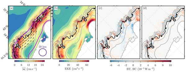
Eddy kinetic energy and energy conversion rates along the Atlantic Water boundary current north of Svalbard

On the continental slope north of Svalbard, the boundary current carrying Atlantic Water (AW) loses heat as it flows eastward. This cooling cannot be fully attributed to atmospheric heat loss or turbulent mixing. Lateral exchange, potentially linked to mesoscale activity, has previously been proposed as a contributing factor, based on limited observations of eddies. Here, we analyse a year-long dataset of hydrography and velocity observations from two mooring arrays, supplemented by output from an eddy-resolving ocean model, to quantify the seasonal variability of eddy kinetic energy (EKE) and baroclinic and barotropic energy conversion rates over time-scales from days to months. Both EKE and conversion rates peak in autumn and winter, coinciding with the strongest boundary current and the warmest AW. Local EKE variability, however, is only weakly associated with conversion rates, suggesting advection from upstream generation sites or unresolved variability from limited measurements. Conversion is mainly baroclinic, through boundary current instability, providing conditions favourable for offshore propagation of warm-core eddies. Modelled conversion rates have a complex spatial structure with substantial values on the offshore, deeper side of the boundary current with comparable contributions from baroclinic and barotropic processes. Resulting mesoscale activity enhances lateral stirring and heat loss from the boundary current, particularly in winter and spring, contributing to the along-stream cooling of AW.

1 Introduction

Atlantic Water (AW) is the primary oceanic source of heat for the Arctic Ocean and plays a central role in shaping its changing physical environment (e.g. Carmack et al., 2015) and ecosystems (Ardyna and Arrigo, 2020). The largest volume of warm AW enters the Arctic Ocean with the West Spitsbergen Current (WSC), which flows through Fram Strait – the main deep gateway connecting the Arctic Ocean to the global oceans (Aagaard et al., 1987; Beszczynska-Möller et al., 2012). The AW flow splits into several poleward and recirculating branches as it approaches the Yermak Plateau (Fig. 1), and the inflow eventually merges downstream and contributes to the Arctic Circumpolar Boundary Current (Rudels et al., 1999). The region north of Svalbard has been shown to have far-reaching signatures in the Arctic Ocean (Polyakov et al., 2017), such as recent changes reported hundreds of kilometres downstream in the Eurasian Basin, including warming of the AW core (Richards et al., 2022), weakening of the halocline and shoaling of the AW (Polyakov et al., 2020a, b), thus affecting the exchange with sea ice and the surface layer.

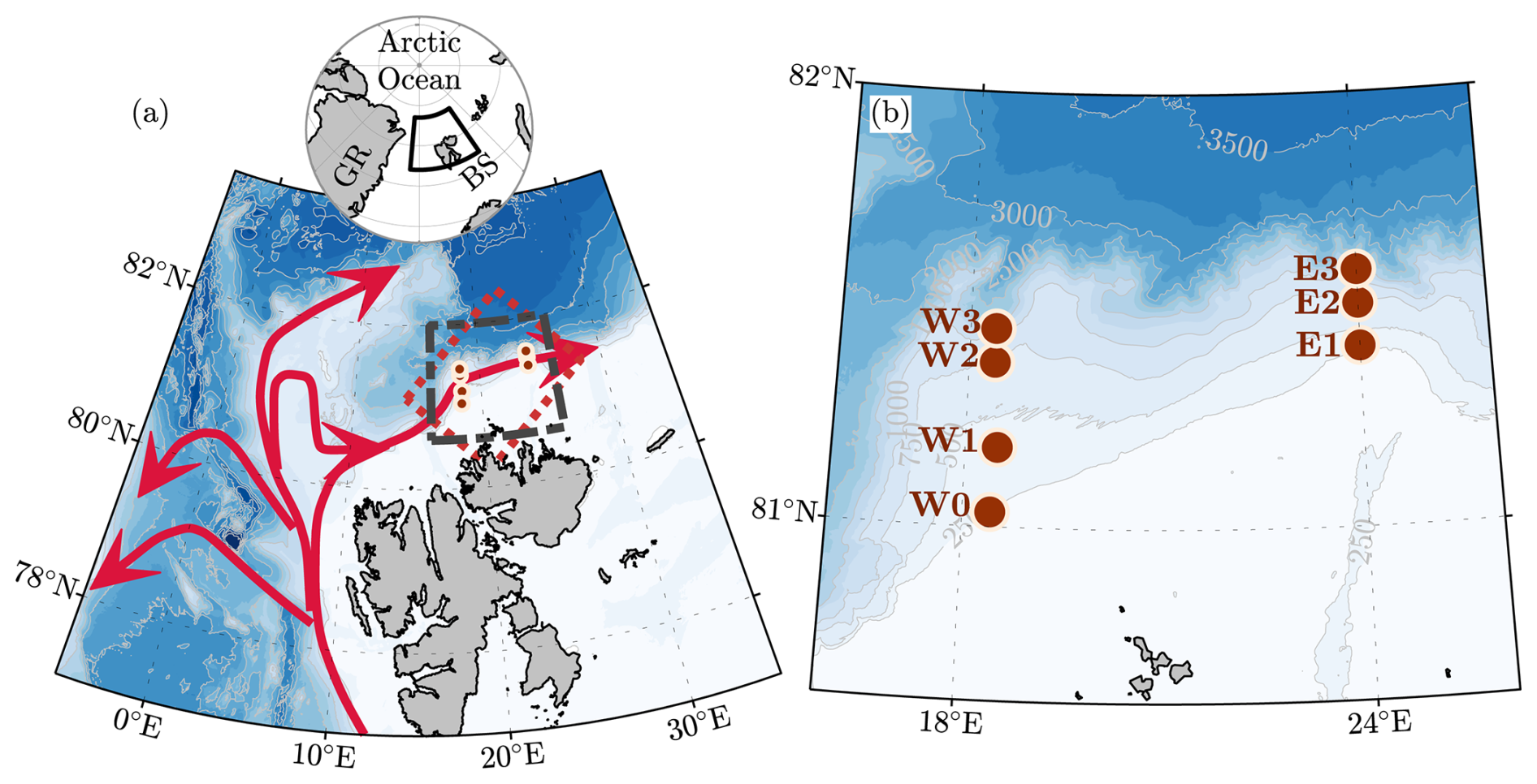
Figure 1 (a) Bathymetry (shading and contours every 500 m; IBCAO version 4, Jakobsson et al., 2020) and circulation of AW (red arrows) in Fram Strait and north of Svalbard. The black box outlines the map in (b), the red box shows the model subdomain. The inset in (a) shows the location in the Arctic Ocean (BS: Barents Sea, GR: Greenland). (b) The study region showing the bathymetry and mooring positions.

The continental slope north of Svalbard is an important area for the modification of AW in the boundary current. The drivers of water mass transformation include air-sea-ice interactions and mixing (Renner et al., 2018; Kolås et al., 2020; Pérez-Hernández et al., 2019; Koenig et al., 2022b), entrainment of surface waters (Richards et al., 2022) and shelf waters (Schauer et al., 1997), and mesoscale variability and eddies (Koenig et al., 2022b; Crews et al., 2018; Wekerle et al., 2020; Athanase et al., 2020; Pérez-Hernández et al., 2017). We define the mesoscale as low Rossby number flows ($\mathit{Ro}=U/fL<\mathrm{1}$, where U and L are the characteristic horizontal velocity and length-scales and f is the Coriolis frequency) that occur on time-scales of days to months and length-scales of 10–100 km. In particular, mesoscale eddies in this region facilitate slope-basin exchange and lateral heat loss (Våge et al., 2016; Pérez-Hernández et al., 2017; Renner et al., 2018). In this study, we investigate the mesoscale variability and energy conversion rates that transfer energy from the mean flow and stratification into eddy energy, using moored observations and a high-resolution numerical ocean model north of Svalbard.

Mesoscale eddies can form through barotropic and baroclinic instabilities of the flow (Killworth, 1980). Barotropic instability may arise from horizontal velocity shear, drawing kinetic energy from the mean flow and converting it into eddy kinetic energy (EKE) (e.g. Cushman-Roisin and Beckers, 2011; Teigen et al., 2010). For a boundary current over a steep slope, the shape of the current determines whether barotropic instability can form. Steep slopes stabilise the current (von Appen et al., 2016), requiring the current to be narrow and fast to become unstable (Håvik et al., 2017). Baroclinic instability, in contrast, may form in regions with a horizontal density gradient, hence strong thermal-wind shear, and converts available potential energy into eddy energy, which enforces flattening of the pycnocline. Bottom slopes also impact (suppress) baroclinic instability (Isachsen et al., 2024).

In the Arctic Ocean, eddies play an important role in variability of inflow water properties and transport and ice–ocean interaction. High mesoscale variability is observed over continental slopes, in Fram Strait, and in the Arctic Circumpolar Boundary Current (von Appen et al., 2022; Wang et al., 2020). These regions, together with the Barents Sea, have relatively higher EKE and baroclinic conversion compared to the rest of the Arctic Ocean (Li et al., 2024). Eddies that shed from unstable fronts along the boundary of the Arctic Ocean transport inflow waters across the basin (Carmack et al., 2015). Eddies also mediate ice–ocean interaction. Under-ice cyclonic eddies can bring AW upward into the surface layer and towards the ice, increasing the heat fluxes and enhancing melting (Müller et al., 2024). Cyclonic eddies may trap and advect sea ice into warmer waters (Manucharyan and Thompson, 2017). Sea ice has been shown to dampen near-surface eddies (Meneghello et al., 2020). The ongoing decline of Arctic sea ice may reduce this effect, causing an increase in near-surface eddy activity and EKE (Armitage et al., 2020; Manucharyan and Thompson, 2022; Müller et al., 2024; Li et al., 2024).

In our study region, north of Svalbard, eddies have been registered both in situ and in models. Scarce observations show evidence for anticyclonic eddies carrying warm anomalies offshore from the shelf break (Våge et al., 2016). These eddies laterally stir and redistribute heat, and thereby contribute to the heat loss from the boundary current (Renner et al., 2018; Koenig et al., 2022b). Estimates of along-path heat loss of AW revealed that turbulent heat fluxes and heat loss to the atmosphere alone could not account for the observed cooling, suggesting a substantial contribution through lateral heat loss (Koenig et al., 2022b). High-resolution model results support this view, showing anticyclonic eddies carrying AW spawning from the boundary current (Crews et al., 2018), propagating offshore towards the deeper basin (Wekerle et al., 2020), facilitating slope–basin exchange and lateral transport of AW. However, the seasonal magnitude and variability of the associated energy conversion rates have not been previously reported from observations in this area.

In the Nansen LEGACY project, the slope north of Svalbard was chosen for targeted studies, including mooring arrays to quantify the properties of the boundary current, specifically its volume transport and along-path cooling (Koenig et al., 2022b), and the mesoscale variability (this study). These detailed observations are analysed here to quantify energy conversion rates and are supplemented using outputs from an eddy-resolving ocean model. The combined results provide insight into where and how the boundary current flow energises variability at mesoscale eddy scales that could contribute to the lateral heat loss from the boundary current.

2 Data and Methods

2.1 Moorings

Ocean temperature, salinity, and horizontal current data were measured at two mooring arrays across the continental slope north of Svalbard (Fig. 1), for approximately one year from September 2018. The western array (18° E) was recovered in September 2019, and the eastern array (24° E) was recovered in November 2019. The data are available from Fer et al. (2022) and have been presented in Koenig et al. (2022b). Each mooring array consisted of one upper slope mooring (W1 and E1) near the 300–400 m isobath, one middle slope mooring (W2 and E2) near the 700 m isobath, and one lower slope mooring (W3 and E3) near the 1200 m isobath, providing a good coverage of the boundary current (Fig. 1b). In addition, a mooring was deployed onshore of the western array (W0). In this study, we used data from the deeper mooring pairs W2–W3 and E2–E3 (Table 1) as the distance within each pair – approximately 9 km – is small enough for calculating lateral gradients (see Sect. 2.3.3).

Table 1 Mooring positions, total depth, and temporal coverage of the deeper mooring pairs used in this study.

Mooring instrumentation coverage and setup, and details of data processing can be found in Koenig et al. (2022a). The vertical instrument coverage at the moorings for September–February and March–August is summarised in Fig. 2. Temperature, salinity, and horizontal current records were checked for inter-consistency and compared and corrected against ship-based profiles taken at mooring deployment/recovery. All time series were hourly averaged (the sampling interval of instruments varied between 5 min and 1 h) and linearly interpolated onto the same hourly time vector. At each hourly time step, instrument depths were obtained by linear interpolation between instruments equipped with a pressure sensor, to account for mooring knockdowns. The data were finally gridded onto a regular (t,z) grid with 1 h temporal and 10 m vertical resolution.

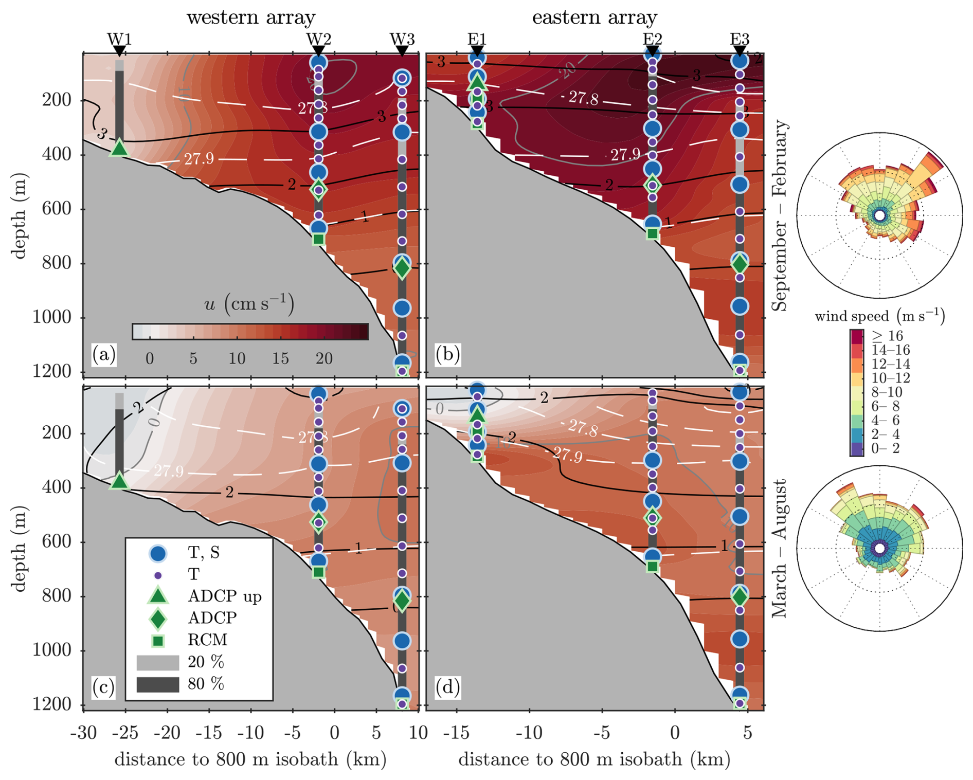
Figure 2 Average along-slope current velocity u (colours) on (a, c) the western and (b, d) eastern mooring arrays during (a, b) autumn and winter (September–February) and (c, d) spring and summer (March–August). Grey contours show velocity every 10 cm s⁻¹, white dashed isopycnals every 0.1 kg m⁻³, and black isotherms every 1 °C. Triangles at the top mark the mooring locations (except W0). Instrumentation is shown at the mooring locations as indicated in the legend. Vertical bars show the current profiling coverage by the acoustic Doppler current profilers (ADCPs) (light grey: 20 % and dark grey: 80 % of the time in each season); large circles indicate conductivity–temperature–depth (CTD) sensors, small circles temperature sensors, triangles upward-facing ADCPs, diamonds pairs of up- and downwards-facing ADCPs, and squares recording current meters (RCMs). Wind roses (right) show the relative frequency of wind direction and speed during (a, b) September–February and (c, d) March–August in the region 18–24.5° E, 81.2–81.7° N, extracted from the Copernicus C3S Arctic Regional Reanalysis (CARRA, Schyberg et al., 2020).

The analysis is based on data from the deeper mooring pairs which provided current profiles with a 5–10 m vertical resolution from the seafloor to approximately 300 m depth. Here, only three levels of density measurements at approximately 300, 500, and 700 m depth were available. Our analysis is therefore based on layer averages over 300 to 700 m (Sect. 2.3.3), focusing on the levels close to the hydrographic sensors to limit the errors from interpolation. For context, we present seasonal mean sections of velocity and hydrography at both mooring arrays (Fig. 2). For computing mean structure of the current velocity and hydrography across the slope, a spline-Laplacian routine was used for interpolation, described in detail in Koenig et al. (2022b). While current measurements cover the water column at W1, there were no temperature and salinity measurements available, and the hydrographic structure over the upper slope was supplemented by historical hydrographic data. The details on the gridding and the associated uncertainties are described in the Appendix of Koenig et al. (2022b).

2.2 Regional Ocean Model

In order to better evaluate and interpret the analysis based on the mooring observations, we used the output from a high-resolution ocean model applying ROMS (Regional Ocean Modeling System; Shchepetkin and McWilliams, 2005) in a domain covering the continental shelf and slope north of Svalbard (Frank et al., 2025). The model used the same configuration as the Norkyst model system documented in Asplin et al. (2020) but was set up with a horizontal resolution of 500 m and 35 vertical stretched bathymetry-following levels. The model configuration also included a sea ice module (Budgell, 2005). The operational ocean forecasting model Barents2.5 (Röhrs et al., 2023) provided boundary conditions including tidal forcing, and the operational weather forecasting model AROME-Arctic (Müller et al., 2017) provided atmospheric input. The model was validated by Frank et al. (2025), and a brief summary of this validation is provided in Appendix B.

The model simulation was initialised in April 2019, and we used two-year daily output from October 2019 to align seasonally with the mooring observations. Hourly saved fields were daily averaged, and the daily fields were then detided for the fortnightly and monthly tidal constituents using UTide (Codiga, 2011). The across-slope structure of the modelled boundary current and hydrography is shown in Fig. B1 and compared with the mooring-based sections in Appendix B.

2.3 Methods for energy analysis

2.3.1 Wavelet analysis

In order to analyse the time variability of energetic frequency bands, we used wavelet transforms with generalised Morse wavelets following Lilly and Olhede (2010, 2012) with the parameters γ=3 for symmetric wavelets (Lilly and Olhede, 2009) and β=9 for a reasonable time and frequency resolution over the relevant time-scales studied here. We denote the wavelet transform of a time series x as W_x and its complex conjugate as ${W_x}^{*}$.

2.3.2 Eddy kinetic energy and energy conversion rates

The calculations of eddy energetics and conversion rates require definition of fluctuations, background conditions, and averaging. We use primed values (e.g. $u^{\prime },{\mathit{\rho }}^{\prime }$) to denote fluctuations from the mean, and an overbar to indicate the background conditions and time averaging (e.g. $\overline{u},\overline{\mathit{\rho }}$). For the moorings, fluctuations were obtained by band-pass filtering the hourly time series using cutoff frequencies corresponding to 35 h and 14 d, and the averaging was done over 30 d moving windows. For the background conditions, we used a low-pass filter with a cutoff frequency corresponding to 30 d. From the model output, primed values were obtained by Reynolds-decomposition, e.g. $u^{\prime }=u-\overline{u}$, where $\overline{u}$ values are 30 d means centred on the 15th of each month and u^′ values are daily fluctuations from the mean.

Eddy kinetic energy density (EKE), the barotropic energy conversion (BT), and the baroclinic energy conversion (BC) rates are defined as

$$\begin{array}{}\text{(1)}& {\displaystyle }& {\displaystyle }\text{EKE}={\displaystyle \frac{\mathrm{1}}{\mathrm{2}}}\left(\stackrel{\mathrm{‾}}{{u^{\prime }}^{\mathrm{2}}}+\stackrel{\mathrm{‾}}{{v^{\prime }}^{\mathrm{2}}}\right),\text{(2)}& {\displaystyle }& {\displaystyle }\text{BT}=-{\mathit{\rho }}_{\mathrm{0}}\left(\stackrel{\mathrm{‾}}{u^{\prime }{u}^{\prime }}{\displaystyle \frac{\partial \overline{u}}{\partial x}}+\stackrel{\mathrm{‾}}{u^{\prime }{v}^{\prime }}\left({\displaystyle \frac{\partial \overline{u}}{\partial y}}+{\displaystyle \frac{\partial \overline{v}}{\partial x}}\right)+\stackrel{\mathrm{‾}}{v^{\prime }{v}^{\prime }}{\displaystyle \frac{\partial \overline{v}}{\partial y}}\right),\end{array}$$

and

$$\begin{array}{}\text{(3)}& {\displaystyle }{\displaystyle }\text{BC}=g{\left({\displaystyle \frac{\partial \overline{\mathit{\rho }}}{\partial z}}\right)}^{-\mathrm{1}}\left(\stackrel{\mathrm{‾}}{u^{\prime }{\mathit{\rho }}^{\prime }}{\displaystyle \frac{\partial \overline{\mathit{\rho }}}{\partial x}}+\stackrel{\mathrm{‾}}{v^{\prime }{\mathit{\rho }}^{\prime }}{\displaystyle \frac{\partial \overline{\mathit{\rho }}}{\partial y}}\right),\end{array}$$

where ρ₀=1027 kg m⁻³ is a reference density, $\stackrel{\mathrm{‾}}{u^{\prime }{u}^{\prime }}$, $\stackrel{\mathrm{‾}}{u^{\prime }{v}^{\prime }}$, and $\stackrel{\mathrm{‾}}{v^{\prime }{v}^{\prime }}$ are eddy momentum fluxes, g is the gravitational acceleration, $\stackrel{\mathrm{‾}}{u^{\prime }{\mathit{\rho }}^{\prime }}$, $\stackrel{\mathrm{‾}}{v^{\prime }{\mathit{\rho }}^{\prime }}$ are eddy density fluxes, $\partial /\partial y$ and $\partial /\partial x$ denote lateral gradients, and $\partial \overline{\mathit{\rho }}/\partial z$ is the mean vertical stratification.

In the model subdomain, EKE, BT, and BC were calculated on the model grid. Then, x and y denote the right-handed orthogonal coordinates in the native model grid, and u and v the velocity components in these directions. For the moorings, x and y denote the local along- and across-slope directions, and u and v the along- and across-slope current components. The coordinate system was rotated with 20° (i.e. counter-clockwise) at the western and −5° (i.e. clockwise) at the eastern array, respectively.

2.3.3 Simplified calculations for conversion rates

Conversion rate estimates from the mooring records were made using simplified forms of Eqs. (2) and (3), with the common assumptions that the across-isobath gradients dominate and that there is no along-isobath variability:

$$\begin{array}{}\text{(4)}& {\displaystyle }& {\displaystyle }\text{BT}=-{\mathit{\rho }}_{\mathrm{0}}\stackrel{\mathrm{‾}}{u^{\prime }{v}^{\prime }}{\displaystyle \frac{\partial \overline{u}}{\partial y}},\text{(5)}& {\displaystyle }& {\displaystyle }\text{BC}=g\stackrel{\mathrm{‾}}{v^{\prime }{\mathit{\rho }}^{\prime }}{\displaystyle \frac{\mathrm{d}z}{\mathrm{d}y}},{\displaystyle \frac{\mathrm{d}z}{\mathrm{d}y}}={\displaystyle \frac{\partial \overline{\mathit{\rho }}}{\partial y}}/{\displaystyle \frac{\partial \overline{\mathit{\rho }}}{\partial z}}.\end{array}$$

In BT (Eq. 4), the lateral gradient was obtained by first differencing of $\overline{u}$ that was layer-averaged over 300–700 m (280–680 m at the eastern array), and the eddy momentum flux was calculated at each mooring and then averaged to be representative of the flux between the moorings. For layer averages, standard error is calculated as $\text{SE}\left(t\right)=\mathit{\sigma }\left(t\right)/\sqrt{n\left(t\right)}$, where n(t) is the number of estimations at time t, and σ(t) is the standard deviation of the n estimations. In BC (Eq. 5), $\mathrm{d}z/\mathrm{d}y$ is the mean isopycnal slope, estimated by the quotient of the across-slope gradient of the mean density $\partial \overline{\mathit{\rho }}/\partial y$ and the mean stratification $\partial \overline{\mathit{\rho }}/\partial z$. The potential density ρ was calculated from gridded T and S fields, at selected depths near the target depths of the sensors, to minimise error from linear interpolation across the halocline.

Calculations of BT and BC require adequate lateral gradient estimations. First, the separation between two moorings must be sufficiently small, limiting the analysis to the deeper moorings pairs. Second, simultaneous measurements at both moorings are needed, constraining the analysis to the 300 to 700 m layer because of substantial data gaps higher in the water column at the deepest moorings. EKE and eddy momentum and density fluxes can be calculated over a broader depth range at all seven moorings (Fig. 1), capturing more of the energetic part of the water column where the data loss was greatest. Their vertical structure is shown in Appendix A.

We conducted additional calculations of BT and BC from the model output using the simplified equations (Eqs. 4 and 5) applied to the time series of velocity and density extracted at grid points representative of the moorings (“virtual moorings”) as well as along 16 and 13 km transects (“segments”) with 24 and 19 grid points across the deeper part of the slope, covering the virtual moorings. Virtual mooring calculations mimic the data and the method used for the in situ moorings, which we compare to the full volume-averaged or segment-averaged conversion rates in order to assess their limitations.

2.3.4 Calculations along the boundary current pathway

We analysed the EKE, energy conversion rates, and eddy temperature fluxes $\left(\stackrel{\mathrm{‾}}{u^{\prime }{T}^{\prime }},\stackrel{\mathrm{‾}}{v^{\prime }{T}^{\prime }}\right)$ obtained from the model to describe the temporal and spatial variability along the pathway of the boundary current. Upon inspection of the model outputs, we identified the 1400 m isobath to be representative of the energetic part of the boundary current on the upper slope. The structure along the isobath is obtained by smoothing the monthly fields using a 2D Gaussian filter with a 20 km length-scale and interpolating the results onto the isobath. The smoothing length-scale ensures that we capture the boundary current structure between, typically, the 800 and 2000 m isobaths.

As an indication of conditions that might allow barotropic instability along the boundary current pathway, we calculate the cross-isobath gradient of potential vorticity, $q_y={\mathit{\beta }}_{\text{topo}}-{\partial }^{\mathrm{2}}\overline{u}/\partial y^{\mathrm{2}}$, where ${\mathit{\beta }}_{\text{topo}}=-\left(f/H\right)\partial H/\partial y$ is the topographic β, H is the water depth, f is the Coriolis parameter, u is the along-stream current velocity component, and y is the across-slope direction. A necessary, but not sufficient, condition for barotropic instability is that q_y must change sign within the domain (Vallis and Maltrud, 1993). Along the 1400 m isobath, we calculated q_y on 20 km lines oriented perpendicular to and centred on the isobath. To approximately visualise this instability condition, we show the product of the minimum and maximum values of q_y calculated along each line, i.e. $f\left(q_y\right)\equiv min\left(q_y\right)\cdot max\left(q_y\right)$, as a change in sign of q_y would result in negative values.

3 Results

3.1 Seasonal and mesoscale variability of the boundary current

Mean structure and seasonal variability of the boundary current observed in the mooring arrays have been reported in Koenig et al. (2022b). Here, we summarise the mean hydrography and current structure relevant to our analysis (Fig. 2) using three-monthly averages grouped into September–February and March–August periods.

The boundary current was on average stronger in September–February, with a velocity core at approximately 100 m depth over the 800 m isobath, carrying AW warmer than 3 °C at a speed exceeding 20 cm s⁻¹ (Fig. 2a and b). In March–August, the velocity core was weaker (10–20 cm s⁻¹), deeper, and relatively diffuse in both vertical and lateral directions (Fig. 2c and d). Water with the highest temperatures, exceeding 2.5 °C, was at 200 m depth seawards of the 500 m isobath, but did not coincide with the deeper velocity core.

The mesoscale variability is demonstrated using records from W2, and shows elevated activity in autumn and winter (Fig. 3), in the same period when the boundary current was strongest and carried the warmest water (Fig. 2a and b). The strongest velocity variability occurred on time-scales between 2 and 6 d and, like the elevated mesoscale activity, was observed in autumn and winter (Fig. 3a and c). From October 2018–January 2019, the offshore velocity component v and the temperature T co-varied on a 3–10 d time-scale (Fig. 3d). At that time, the current core was located near the 800 m isobath, close to W2, and carried AW (Fig. 2a).

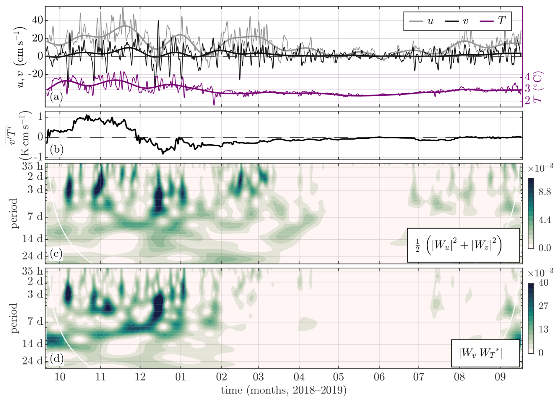
Figure 3 Time series of (a) along-slope and across-slope current velocity u, v (left axis), and temperature T (right axis, purple) measured at 250 m depth at the western mooring W2 (a level in the core which consistently has both temperature and velocity measurements), low-passed filtered at 35 h (thin curves) and 30 d (thick curves). Corresponding (b) offshore eddy temperature flux $\stackrel{\mathrm{‾}}{v^{\prime }{T}^{\prime }}$ (positive for warm anomalies towards deeper water and cold anomalies towards shallower water), (c) wavelet power spectrum, $\frac{\mathrm{1}}{\mathrm{2}}\left({\left|W_u\right|}^{\mathrm{2}}+{\left|W_v\right|}^{\mathrm{2}}\right)$, and (d) wavelet cross-spectrum $\left|W_v{W_T}^{*}\right|$ between v and T. The cone of influence (solid white curve) in (c) and (d) indicates the areas affected by boundary effects.

The offshore eddy temperature flux, $\stackrel{\mathrm{‾}}{v^{\prime }{T}^{\prime }}$, at 250 m depth was positive in the autumn of 2018, peaking in mid-November, and became negative in December 2018 (Fig. 3b), consistent with mesoscale activity driving cross-isobath heat transport. Averaged over September–November 2018, $\stackrel{\mathrm{‾}}{v^{\prime }{T}^{\prime }}$ at W2 was positive at depths 150 to 350 m, spanning the temperature core. At W3, the eddy temperature flux in the upper water column could not be calculated in autumn due to mooring knockdown, but was positive at and below 400 m depth (not shown). The eddy temperature flux divergence between W3 and W2 was over four times higher in autumn and winter (September–February) than in spring and summer (March–August; not shown), suggesting stronger lateral heat loss from the boundary current in autumn and winter. While the relatively higher eddy temperature flux and its divergence in autumn and winter indicate increased mesoscale activity, we cannot directly quantify net lateral heat transport because the rotational and the divergent components of the flux could not be separated (Marshall and Shutts, 1981; Guo et al., 2014).

3.2 Energetics and conversion rates from mooring data

Despite their limited spatial coverage and sampling volume, the moorings enable year-round estimates of eddy kinetic energy and associated energy conversion rates. EKE and BT, together with its contributing terms, are shown in Fig. 4. BC and its contributing terms are shown in Fig. 5. To provide context for the magnitudes of conversion rates and their effect on changes in EKE, note that a conversion rate of $\mathrm{1}\times {\mathrm{10}}^{-\mathrm{5}}$ W m⁻³ sustained over one day would produce $\mathrm{1}\times {\mathrm{10}}^{-\mathrm{3}}$ J kg⁻¹ corresponding to an EKE increase of 10 cm² s⁻².

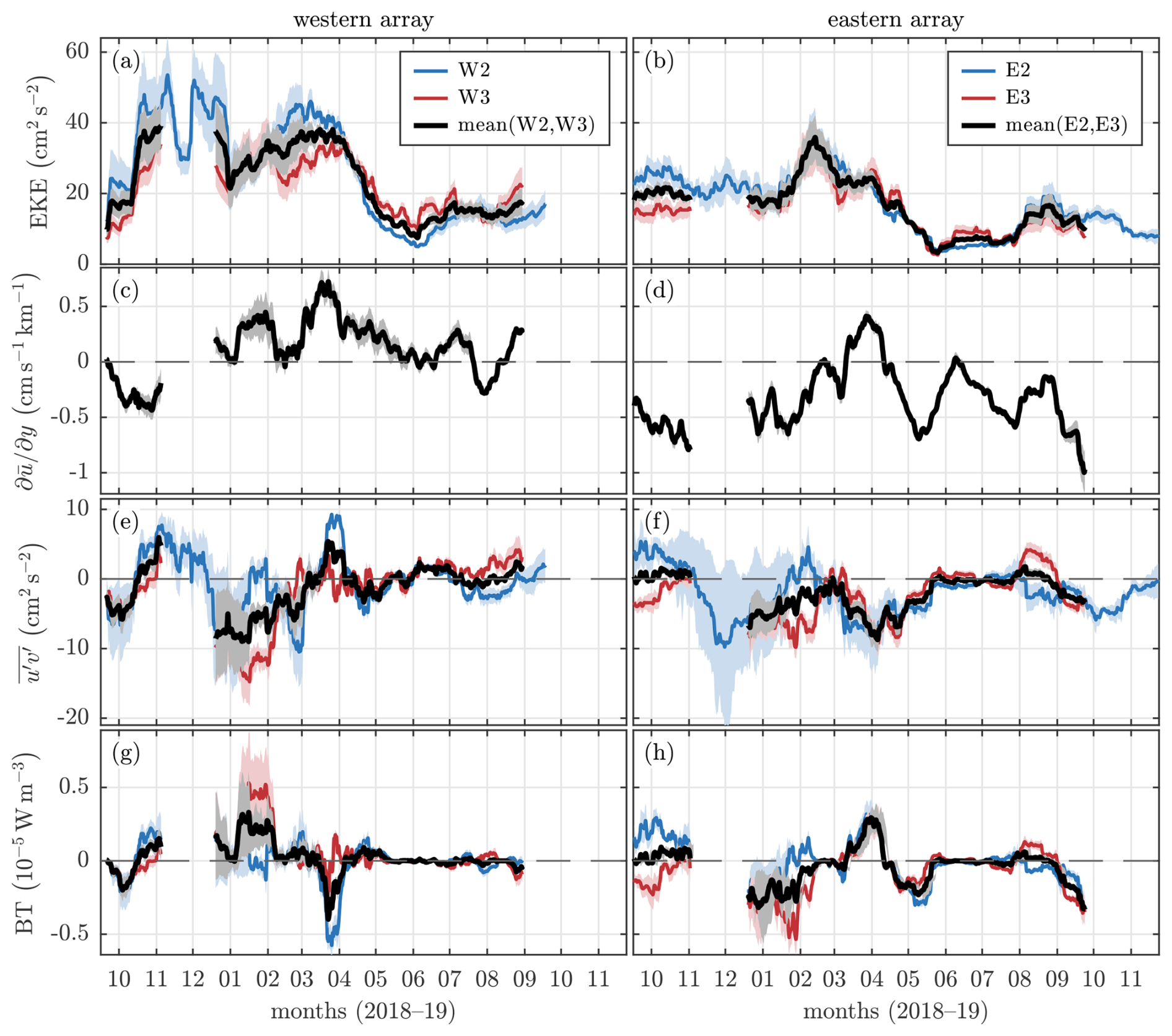
Figure 4 Time series of (a, b) EKE, (c, d) lateral shear of the mean along-slope current, (e, f) eddy momentum flux, and (g, h) BT at the (left) western and (right) eastern arrays. Blue curves are values at W2 and E2, red curves at W3 and E3, and black curves for the average between the pair of moorings. Shading shows standard error calculated from estimates at 100 m intervals in the depth range 300–700 m.

Several features are consistent at both mooring arrays. EKE was higher in autumn and winter than in spring and summer (Fig. 4a and b), with values at 300 m depth approximately four times larger than at 700 m (not shown). In contrast, BT remained weak year-round relative to the conversion rate expected from the observed EKE variability (Fig. 4g and h). It was negligible in summer and otherwise fluctuated within $\pm \mathrm{0.5}\times {\mathrm{10}}^{-\mathrm{5}}$ W m⁻³. The persistently low BT reflects both cancellation of oppositely signed momentum fluxes (Fig. 4e and f) and periods of weak velocity shear (Fig. 4c and d). BC was generally largest in autumn and winter at both sites, ranging from $-\mathrm{3}\times {\mathrm{10}}^{-\mathrm{5}}$ to $\mathrm{4}\times {\mathrm{10}}^{-\mathrm{5}}$ W m⁻³, and decreasing to near-zero values in spring and summer (Fig. 5e and f). BC was generally strongest at the uppermost measurement level (310–320 m), where variability in density and cross-slope velocity was greatest, and decreased with depth (Fig. 5c and d). Despite these similarities, BC estimates showed substantial variability between depths and moorings, particularly in autumn and winter, primarily due to differences in eddy density fluxes despite being measured only 100 m apart vertically, e.g. in October and November 2018 (Fig. 5c and d).

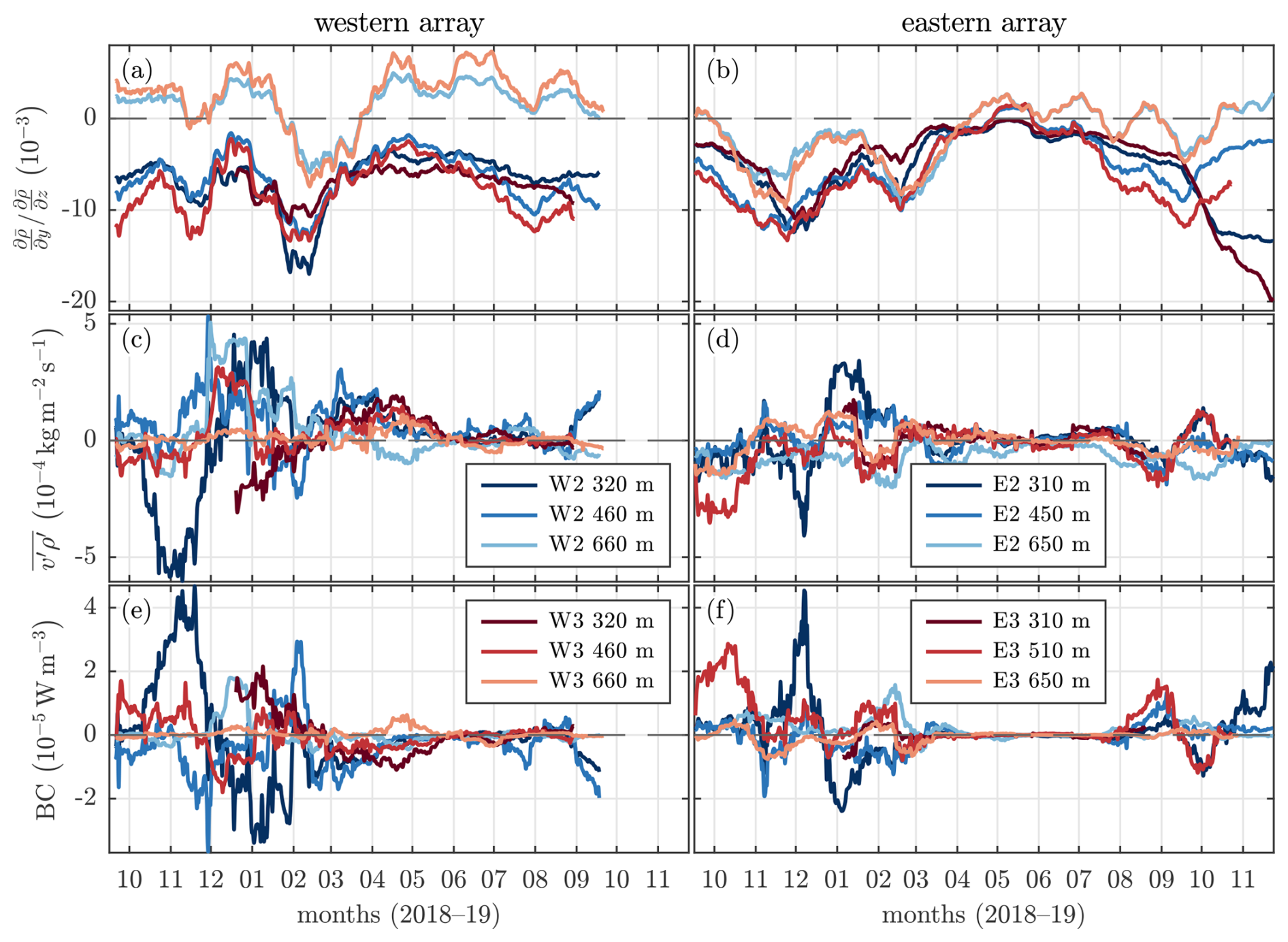
Figure 5 Time series of (a, b) isopycnal slope, (c, d) eddy density flux, and (e, f) BC at the (left) western and (right) eastern arrays. A positive isopycnal slope occurs when density decreases with offshore distance.

At the western array, the autumn- and wintertime EKE reached nearly 40 cm² s⁻², and decreased to below 20 cm² s⁻² in summer (Fig. 4a). BT was generally weak, with two notable exceptions. In January 2019, BT was positive (Fig. 4g). Based on estimates at 100 m intervals (not shown), the values at the uppermost level (300 m) reached $\mathrm{1}\times {\mathrm{10}}^{-\mathrm{5}}$ W m⁻³ driven by negative momentum fluxes combined with positive shear. This signal weakened with depth, reducing the layer-average BT. In late March 2019, a second event occurred, when strong positive velocity shear and positive momentum flux at W2 produced a similarly large but negative and shorter-lived BT (Fig. 4g, c, and e).

The eastern array had generally lower EKE than the western array, but with a comparable seasonal contrast. BT showed a similar overall behaviour to the western array. Typically low values increased in two events, but with opposite signs to the western array. BT was negative in January 2019 due to modest momentum fluxes and shear, while from late March to early April 2019, BT was positive due to a period of negative momentum fluxes and an offshore displacement of the boundary current (Fig. 4h, d, and f). During the February EKE maximum, BT remained negligible due to near-zero shear and momentum fluxes.

At the western array, the most notable BC event occurred at 320 m at W2 from mid-October through November 2018. BC increased from negligible values to $\mathrm{4}\times {\mathrm{10}}^{-\mathrm{5}}$ W m⁻³ and remained elevated for nearly a month. This event coincided with a strong mean current, high EKE (Fig. 4a), a modest and persistent negative isopycnal slope, and an elevated eddy density flux from an increased variability and covariance of v and ρ, with dominant periods of 2–10 d (similar to Fig. 3d). During and following this event, EKE at W2 remained high, peaking at 88 cm² s⁻² at 300 m depth. However, such concurrent increases in EKE and BC were not commonly observed. A similar but shorter-lasting event occurred at 310 m depth at E2 from mid-November to early December 2018 (Fig. 5f).

In summary, current strength, temperature variability, EKE, eddy momentum and density fluxes, BC, and to a lesser extent BT, were all generally stronger in autumn and winter than in spring and summer. Although the measurements do not resolve the upper ocean and surface layer, the available vertical coverage indicates a tendency for enhanced EKE, BT, and BC at the uppermost measurement levels. While EKE was often elevated during periods of higher fluxes and BC, the relationship between them was neither consistent nor robust.

Advection of eddies past the moorings complicates the interpretation of our estimates in several ways. A fraction of the calculated EKE may be attributed to eddies advected by the mean flow, adding to the local conversion from mean to eddy energy, potentially leading to an overestimation of locally generated EKE. In addition, the use of a band-pass filter to estimate fluctuations may attenuate contributions from mesoscale features when the filter cutoff exceeds the eddy advection time scale. The advection time scale is 24–40 h, based on along-slope velocities of 10–15 cm s⁻¹ and an eddy lateral length scale of twice the baroclinic Rossby radius of deformation (∼7 km). This range overlaps with, and partly exceeds, the 35 h cutoff used in the EKE calculations. Alternative calculations using a shorter cutoff of ≈24 h, excluding the diurnal tidal band while retaining most mesoscale variability, show no significant differences (Appendix C; Fig. C1a and b).

3.3 Energetics and conversion rates from the ocean model data

We analyse output from the high-resolution model to assess whether the conversion estimates using the simplified expressions for BT and BC, based on limited depth levels and mooring locations, are representative of a broader region. To do so, we calculate EKE, BT, and BC using the full conversion terms (Eqs. 2 and 3) and vertically average over 100–2000 m to obtain their spatial structure (Fig. 6 and Sect. 3.3.1). We then show the temporal evolution of the energetics along the boundary current pathway by averaging over a 20-km diameter region centred on the 1400 m isobath (Fig. 7 and Sect. 3.3.2). Additionally, we apply the simplified formulations (Eqs. 4 and 5) to velocity and density time series extracted at virtual moorings, using the same method as for the moorings (Fig. 8 and Sect. 3.3.3). These results are compared with both the observational estimates and the spatially averaged values along the boundary current pathway.

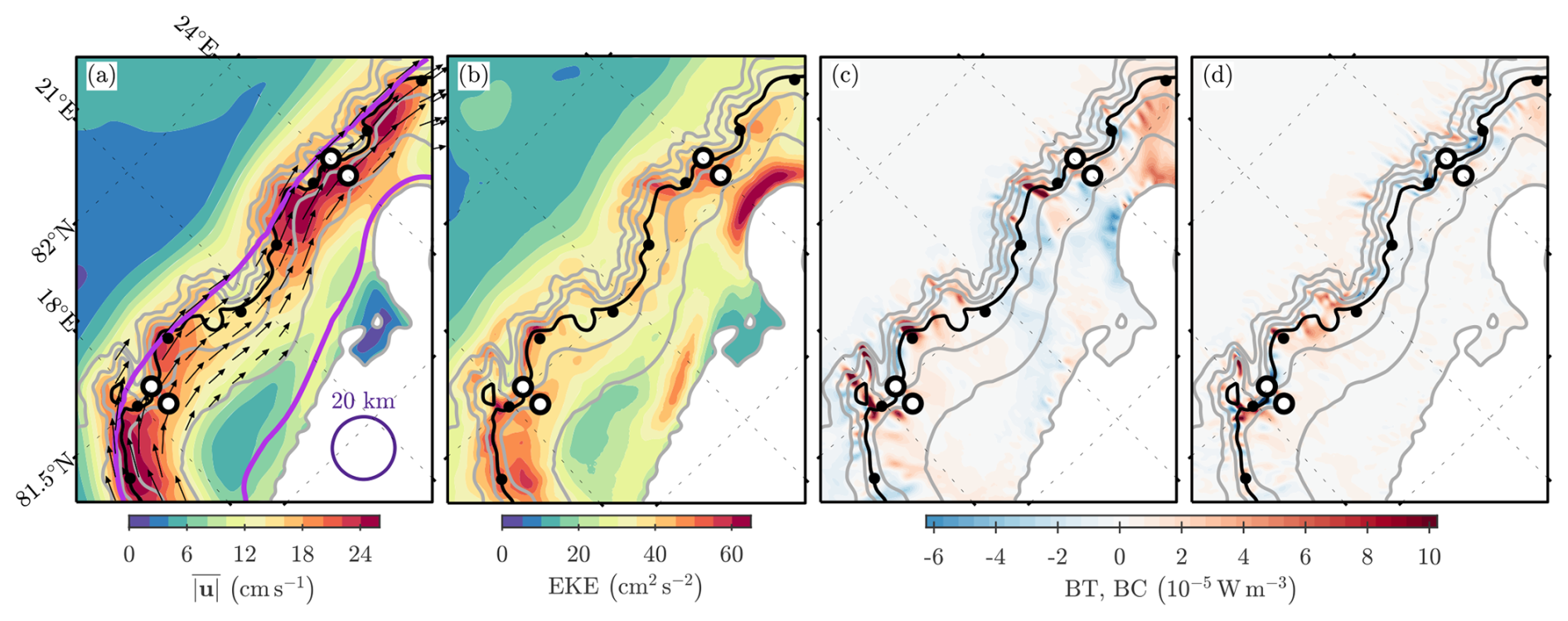
Figure 6 Maps of the two-year mean (October 2019–September 2021) model fields, averaged from 100 m to the seafloor or to 2000 m depth if deeper, for (a) current speed, (b) EKE, (c) BT, and (d) BC. To highlight the AW boundary current in (a), velocity vectors are shown between the 600 and 2800 m isobaths, and the 100–500 m layer-averaged 2 °C isotherm is shown with purple curves. The positions of the virtual moorings are marked with circles. Isobaths are drawn at 400 m intervals from 200 to 2600 m (grey), and the 1400 m isobath is highlighted in black. Black dots mark the distance along the 1400 m isobath every 25 km starting at 0 km with the first dot. In (a), the circle at 20° E of diameter 20 km shows the length-scale of the spatial filtering applied in Fig. 7.

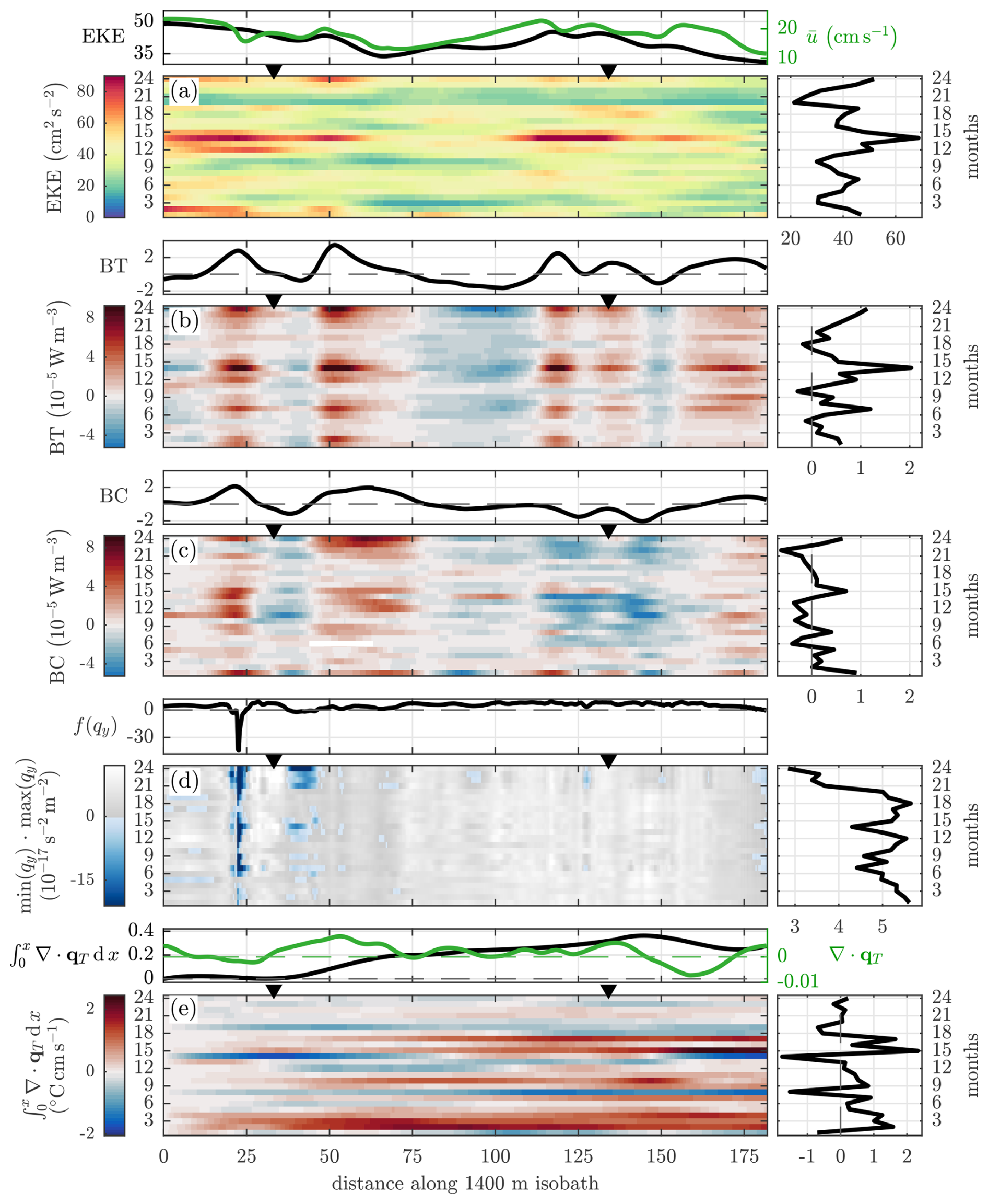
Figure 7 Spatio-temporal evolution along the 1400 m isobath of modelled (a) EKE, (b) BT, (c) BC, (d) $f\left(q_y\right)\equiv min\left(q_y\right)\cdot max\left(q_y\right)$ (negative values indicate a cross-isobath change of sign of the lateral PV gradient q_y), and (e) cumulative along-isobath integral of eddy temperature flux divergence, ${\int }_{\mathrm{0}}^x\mathrm{\nabla }\cdot {\mathit{q}}_T\mathrm{d}x$, where ${\mathit{q}}_T=(\stackrel{\mathrm{‾}}{u^{\prime }{T}^{\prime }},\stackrel{\mathrm{‾}}{v^{\prime }{T}^{\prime }})$. Each group of panels includes the spatio-temporal field (colours), its time-average (top), and its along-isobath average (right), except in panel (e) where the panel on the right shows the along-isobath integral evaluated at the end of the isobath, ca. 180 km. In addition, time-averaged $\overline{u}$ (a) and ∇⋅q_T (e) are shown (green, top panels, right axes). Temporal averaging is 1 month and the spatial smoothing is 20 km. October corresponds to months 1 and 13, April to months 7 and 19. Triangles mark approximate locations of the virtual moorings. Distance-axis intervals every 25 km correspond to the dots on the 1400 m isobath in Fig. 6. All variables are layer-averaged from 100 to 2000 m or the seabed, except ∇⋅q_T which is from 100 to 500 m.

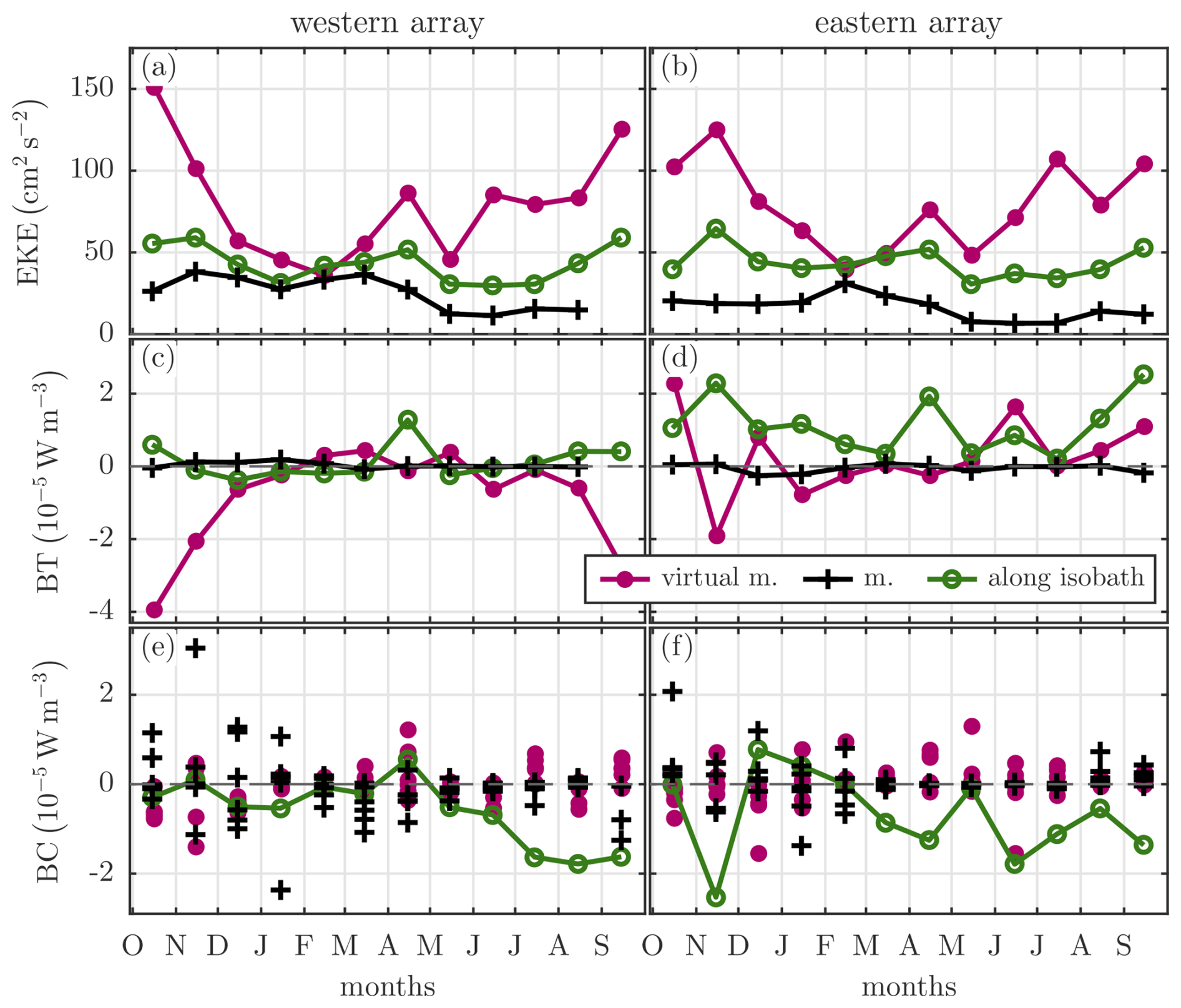
Figure 8 Time series of (a, b) EKE, (c, d) BT, and (e, f) BC from in situ moorings (black pluses), from the model using virtual moorings (purple dots), and the average along the 1400 m isobath near moorings (green open circles). The two model years were averaged together. In (e, f), BC is shown for the same levels as the moorings (Fig. 5). The in situ mooring time series are as in Figs. 4 and 5 but monthly averaged.

3.3.1 Mean spatial distribution

The core of the AW boundary current is evident in the vertically and temporally averaged current speed, located over the upper continental slope between the 1000 and 1400 m isobaths, with peak velocities exceeding 24 cm s⁻¹ (Fig. 6a). The mooring pairs capture this boundary current structure well. Waters warmer than 2 °C within the 100–500 m depth range extend from the lower continental slope across the current core and onshore toward the shelf, where the mean flow gradually weakens. Applied 20 km diameter averaging along the 1400 m isobath covers the core of the boundary current carrying AW and captures the energetic part of the slope. EKE values along the slope, averaged over 2 years, were typically 30–50 cm² s⁻², with higher values up to 60 cm² s⁻² around and upstream of both mooring arrays (Fig. 6b).

Time-averaged BT had strong spatial variability along the slope (Fig. 6c). The largest maxima were found on the steep slope seaward of the 800 m isobath, with particularly elevated values in the region of complex bathymetry upstream of the western array, where local values reached 15–$\mathrm{30}\times {\mathrm{10}}^{-\mathrm{5}}$ W m⁻³ (Fig. 6c, these values exceed the colorbar range). Other strong positive regions were found near the 1400 m isobath, approximately 20 km downstream of the western array ($\mathrm{25}\times {\mathrm{10}}^{-\mathrm{5}}$ W m⁻³), and approximately 20 km upstream of the eastern array ($\mathrm{15}\times {\mathrm{10}}^{-\mathrm{5}}$ W m⁻³). The zones of BT maxima were anisotropic, elongated in the across-isobath direction. Aside from the strong positive maxima, time-averaged BT alternated in sign along the slope, characterized by transitions between local minima and maxima, often associated with variations in slope geometry and isobath curvature.

BC had comparable spatial variability and magnitude to BT (Fig. 6d). The largest time-mean BC values were also found on the steep slope near the western array. Some of these areas were co-located or overlapping with the BT maxima. Local peak values reached 11–$\mathrm{24}\times {\mathrm{10}}^{-\mathrm{5}}$ W m⁻³. A pronounced BC maximum occurred near the 1400 m isobath 20 km downstream of the western array, coincident with the strong BT maximum there, though with roughly half the magnitude. Another conversion site ($\mathrm{24}\times {\mathrm{10}}^{-\mathrm{5}}$ W m⁻³), also co-located with BT, was upstream of the western array.

Several of the regions along the slope that were energetic on average were associated with maxima in time-mean conversion rates. In some energetic locations, BT and BC were co-located or overlapping, while in others, primarily one of the conversion types dominated.

3.3.2 Structure along the boundary current pathway

Along the 1400 m isobath, EKE, BT, and BC varied spatially and temporally (Fig. 7). Time-mean EKE was slightly elevated over broad regions near both mooring arrays, with the highest mean value of 50 cm² s⁻² occurring 30 km upstream of the western array (Figs. 6b, and 7a). Monthly averages over the full 180 km extent of the isobath ranged from 20 cm² s⁻² in month 20 (May) to 65 cm² s⁻² in month 14 (November).

When averaged along the 1400 m isobath over the full period, BT was $\mathrm{0.47}\times {\mathrm{10}}^{-\mathrm{5}}$ W m⁻³, one order of magnitude larger than BC ($\mathrm{0.05}\times {\mathrm{10}}^{-\mathrm{5}}$ W m⁻³). Both conversion terms displayed substantial along-isobath variability. Time-mean BT ranged from a negative value of $-\mathrm{1.7}\times {\mathrm{10}}^{-\mathrm{5}}$ W m⁻³ in the region between the mooring arrays to a maximum positive rate of $\mathrm{3.5}\times {\mathrm{10}}^{-\mathrm{5}}$ W m⁻³ located 20 km downstream of the western mooring array. A secondary BT maximum of $\mathrm{2.8}\times {\mathrm{10}}^{-\mathrm{5}}$ W m⁻³ was located about 10 km upstream of the western array. Further east, two additional local maxima were found 15 km upstream of the eastern array ($\mathrm{2.5}\times {\mathrm{10}}^{-\mathrm{5}}$ W m⁻³) and at the array ($\mathrm{1.4}\times {\mathrm{10}}^{-\mathrm{5}}$ W m⁻³). Averaged along the isobath, BT reached a maximum of $\mathrm{2.0}\times {\mathrm{10}}^{-\mathrm{5}}$ W m⁻³ in month 14, which coincided with the EKE peak. The minimum value of $-\mathrm{0.3}\times {\mathrm{10}}^{-\mathrm{5}}$ W m⁻³ occurred in month 10 (July). Overall, no clear seasonality was observed.

The time-mean BC varied within $\left(-\mathrm{2.1},+\mathrm{2.1}\right)\times {\mathrm{10}}^{-\mathrm{5}}$ W m⁻³. The largest positive BC was approximately 10 km upstream of the western array, coincident with a BT local maximum, and within a broad region extending 15–40 km downstream of the western array, where BC remained above $\mathrm{1.0}\times {\mathrm{10}}^{-\mathrm{5}}$ W m⁻³. In contrast, BC was negative on average near the eastern array. Averaged along the isobath, BC varied within $\left(-\mathrm{0.6},+\mathrm{0.9}\right)\times {\mathrm{10}}^{-\mathrm{5}}$ W m⁻³.

Although there were occasional coincidences between peaks in EKE and conversion rates on the 1400 m isobath, the variability of EKE generally did not match the local conversion rates. This lack of a robust relation between EKE variability and conversion rates mirrors the findings in the mooring observations and suggests that increasing EKE in a region does not necessarily indicate that strong local energy conversion is taking place. While there is not a conclusive, direct correspondence between local conversion rates and EKE variability, several segments along the isobath exhibit statistically significant correlations (not shown; Pearson's correlation coefficient, r, ranging from 0.65 to 0.92). In particular, BT and EKE are significantly positively correlated in regions where BT is mainly positive (directly upstream and 20 km downstream of the western array, and across a broad region surrounding the eastern array (Fig. 7b)). Near the western array, the predominantly positive BC also shows a positive but weaker correlation with EKE, (r from 0.51 to 0.67).

The cross-isobath gradient of the effective potential vorticity, q_y, suggests some regions along the boundary current may be susceptible to barotropic instability. To diagnose this, we evaluate at each along-isobath point the product of the minimum and maximum values of q_y across the 1400 m isobath, f(q_y), which visualises whether q_y changes sign (Fig. 7d; also discussed further in Sect. 4.3). Several zones show near-zero or negative values of f(q_y), implying sign changes in q_y. These include a narrow region 10 km upstream of the western array and a broader zone 10 km downstream, suggesting that the necessary condition for barotropic instability may be locally satisfied during the two-year period. In other zones, f(q_y) alternates in sign, indicating that topographic β was small enough to be outweighed by the curvature of the current at the 1400 m isobath in some months. Positive BT is also found in regions where the necessary condition for barotropic instability is not met, indicating that eddy–mean flow interaction may occur in regions that are not locally unstable.

The divergence of eddy temperature flux integrated along the 1400 m isobath (Fig. 7e) has pronounced temporal variability, ranging from −1.8 to 2.3 °C cm s⁻¹, with a mean value of 0.3 °C cm s⁻¹. The five months with the largest integrated eddy temperature flux divergence occurred between November and February. Averaged in time, the cumulative integral of eddy temperature flux divergence increases from near the western mooring array to 10 km downstream of the eastern array (Fig. 7e, upper panel, left axis). The largest contributions to the cumulative integral are from a broad zone extending downstream from the western mooring array (35–70 km along the isobath) and a narrower zone centred on the eastern array (125–140 km; Fig. 7e, upper sub-panel, right axis). The broad zone starting from the western array coincides with areas where both BT and BC are positive on average (Fig. 7b and c), while the more localized smaller maximum near the eastern array is approximately co-located with the local BT maximum there.

3.3.3 Variability at the virtual moorings compared to in situ moorings and along-isobath estimates

The virtual moorings tended to overestimate the magnitude and variability of EKE relative to the spatially averaged model estimates along the 1400 m isobath sampled at the mooring sites (Fig. 8a and b). EKE was for example on average 1.8 times higher, and at most 4 times higher, at the virtual mooring than in the spatially averaged along-isobath estimates. In contrast, EKE estimates from the virtual moorings match well those obtained from cross-slope segments spanning the vertical and lateral extent of the moorings, as well as from longer segments covering most of the water column (not shown), indicating that point-based sampling can capture the energetics of a broader cross-slope region. EKE in the model was generally larger than the observed EKE, especially during summer when observed values were reduced to approximately half of the autumn- and winter values.

BT estimated from the virtual moorings was generally larger in magnitude than both the along-isobath estimates and, in particular, the in situ mooring estimates (Fig. 8c and d). BC estimates from the virtual moorings showed variability comparable to the in situ observations and showed similarly sensitivity to sampling depth and the choice of mooring pair (Fig. 8e and f). As with BT, virtual-mooring BC estimates diverged from the spatially averaged values. While BT from the virtual moorings broadly agreed with segment-based estimates, BC showed larger disagreement (not shown).

Differences between the model-based and observational estimates could be attributed to the different time periods covered, the representativeness of mooring locations relative to the boundary current, isopycnal slopes and shear, and potential shortcomings of the model in representing the meso- and submesoscale processes. EKE and conversion rate estimates using the full equations for the conversion rates and averaging over the full depth and across the region, differed substantially from the simplified virtual mooring and segment-based estimates, highlighting the effects of the calculation method and the importance of adequate volume-averaging.

4 Discussion

4.1 EKE and conversion rates

We observed higher EKE during autumn and winter from the mooring observations (Fig. 4a and b). This agrees with Crews et al. (2018) who found higher EKE between October and March in a high-resolution model and with Koenig et al. (2022b) who found increased geostrophic surface EKE in the autumn and winter months. Upstream at the 78°50^′ N mooring array, the WSC is most energetic from December to May, with a peak in February (von Appen et al., 2016). In AW inflow regions, such as the Barents Sea Opening, Fram Strait, and the western Nansen Basin, wintertime EKE can be relatively higher. This is attributed to the typically lower sea ice cover in these areas, which permits stronger wind forcing and supports weaker stratification and higher instability (von Appen et al., 2022).

During the same periods of elevated EKE in autumn and winter, we also observed larger energy conversion, with BC as the dominant contribution (Figs. 4g and h and 5e and f). The important role of BC in autumn and winter seen in the mooring observations is supported by the model, lending confidence to the simplified calculations from the moorings. Previous studies from upstream regions in Fram Strait and west of Spitsbergen have similarly shown that the boundary current is baroclinically unstable (Teigen et al., 2011; von Appen et al., 2016; Wekerle et al., 2020; Fer et al., 2023). The high wintertime EKE in the WSC has been linked to baroclinic instability due to weak stratification and a stronger vertical shear (von Appen et al., 2016). Similarly, in the Eurasian Basin, Müller et al. (2024) reported a spatial agreement between EKE and BC, suggesting that baroclinic instability supplies eddy energy locally. Our finding that both EKE and BC are greater in autumn and winter indicates that baroclinic instability may similarly drive higher EKE north of Svalbard as well.

While BC was stronger in the mooring observations, the volume-averaged conversion rates in the model show similar contributions of BT and BC (Fig. 6c and d). Averaged along the boundary current path, BT was comparable to and larger than BC for most of the time (Fig. 7b and c). Considering the uncertainties and limitations of point-based estimates of conversion rates, highlighted by the limited ability of the virtual moorings to reproduce the volume-averaged conversion rates along the boundary current pathway (Sect. 3.3.3 and Fig. 8), we may assume there can be a substantial contribution to energy conversion from barotropic instability. Upstream of our mooring site, the boundary current west of Spitsbergen has been shown to be barotropically unstable (Teigen et al., 2010), and the results of Wekerle et al. (2020) also indicate that barotropic conversion is non-negligible.

Conversion rates have been estimated in several other studies using mooring observations and models. Across the pathway of the WSC in Fram Strait, conversion rates inferred from moored observations were highest near the shelf break during winter, with a pronounced seasonal cycle, peaking in February and reaching its minimum in August (von Appen et al., 2016). Their largest monthly mean BT, $\mathrm{2.5}\times {\mathrm{10}}^{-\mathrm{5}}$ W m⁻³ at 75 m depth in February, is about ten times higher than our layer-averaged maximum during January 2019 at the western array. At the same location, their BC value reaches $\mathrm{15}\times {\mathrm{10}}^{-\mathrm{5}}$ W m⁻³, which exceeds our largest monthly mean, $\mathrm{2.9}\times {\mathrm{10}}^{-\mathrm{5}}$ W m⁻³ at 320 m in November. In our data, both BT and BC tended to be larger in the shallower part of the 300–700 m depth range, so it is plausible that values at 75 m could be closer to those of von Appen et al. (2016). It should be noted that we used slightly different passbands than von Appen et al. (2016) to obtain fluctuations. A comparison between choices of passbands and filters is shown in Appendix C. If we use their passband of 48 h to 30 d instead of our 35 h to 14 d, our November-mean BC increases by 25 %. Conversion rates in Fram Strait estimated using two high-resolution models (Wekerle et al., 2020), reach magnitudes of $\mathrm{5}\times {\mathrm{10}}^{-\mathrm{5}}$ m³ s⁻³ along the slope. Depth-integrated values in m³ s⁻³ are numerically equivalent to depth-averaged values with units W m⁻³ for a ∼1000 m-thick layer of seawater with density ∼1000 kg m⁻³.

On the southern flank of the Yermak Plateau at 80° N, further downstream of the mooring observations of von Appen et al. (2016), Fer et al. (2023) estimated conversion rates from mooring records. Similar to our results, they observed that both BT and BC were highly variable in depth and time, with no consistent or strong correlation with EKE. Their observed EKE levels exceeded what would be expected from the local conversion rates and could be partly accounted for advection from an energetic region upstream of the moorings reported in von Appen et al. (2016).

Negative conversion rates, observed in both our mooring records (lasting weeks) and the model (lasting months in some regions), have also been reported in other regions (e.g. Spall et al., 2008; Håvik et al., 2017; Wekerle et al., 2020; Fer et al., 2023). Theoretically, negative BT implies a transfer of energy from eddies to the mean flow, while negative BC implies energy transfer that steepens isopycnals by lifting denser water toward the shelf. Our observations provide some support for these interpretations. For example, a period of negative BC in January–February 2019 was followed by an increase in isopycnal slope (Fig. 5c and a). In the model, a wide zone between 80 and 110 km along the isobath with predominantly negative BT (Fig. 7b), shows a significant negative correlation (r −0.47 to −0.72) with the along-slope current velocity (not shown). Here, decreasing BT is associated with increasing current strength, consistent with a transfer of energy from eddies and to the mean flow. Correspondingly, the mean velocity transitions from below- to above-average values downstream (Fig. 7a, right axis of upper panel), suggesting a local strengthening of the boundary current. However, this relation between negative BT and an increase in $\overline{u}$ is not found in all regions. Due to uncertainties in the estimates from the moorings, we cannot determine whether the observed change in the isopycnal slope is a direct consequence of negative BC or a coincidental alignment. However, the occurrence of negative conversion rates in both observations and high-resolution models supports the interpretation that energy can be transferred to the mean flow or into available potential energy.

4.2 Mesoscale activity and heat loss from the boundary current

Understanding heat loss from AW along the boundary current is key to regional climate and oceanography north of Svalbard, with implications for the broader Arctic Ocean. Koenig et al. (2022b) estimated the seasonal evolution of along-stream heat loss of AW between the western and the eastern mooring arrays and showed that air–sea heat fluxes alone cannot account for the observed cooling rates in winter, spring, and summer. This implies that additional mechanisms contribute to the along-stream heat loss of AW, such as lateral exchange proposed by Crews et al. (2018) and Kolås et al. (2020).

Several observations from the slope north of Svalbard indicate the presence of such lateral processes. Temperature variability exhibited an onshore–offshore mode with a 6–7 d periodicity that was correlated with across-slope velocity variability, and surface geostrophic EKE was elevated near the current core (Koenig et al., 2022b). Anticyclonic eddies are a likely agent for this exchange. Limited observations north of Svalbard showed anticyclones carrying warm anomalies offshore from the boundary current (Våge et al., 2016) and other eddy features linked to baroclinic instability (Pérez-Hernández et al., 2017). Anticyclonic eddies carrying AW or warm anomalies have also been identified in high-resolution modelling studies both north of Svalbard (Crews et al., 2018) and upstream (Wekerle et al., 2020). The model results presented here also indicate substantial conversion rates both near the mooring sites and further offshore (Fig. 6).

Seasonal contrasts further point to a role for mesoscale processes in the heat budget. In autumn, along-stream heat loss can largely be explained by direct atmospheric cooling, when the AW core is warm, shallow, and the region is ice-free (Koenig et al., 2022b). In winter, however, along-stream heat loss increases substantially while the AW core subducts and becomes less exposed to the atmosphere. During this period, EKE remains elevated, suggesting that lateral exchange associated with mesoscale activity becomes more important. In spring, surface heat loss is strongly suppressed by sea ice, while mesoscale activity persists at reduced levels, again indicating a contribution from eddy-driven lateral exchange. Consistent with this interpretation, eddy temperature flux divergence estimated from the moorings (Sect. 3.1) indicates stronger lateral heat loss from the boundary current in autumn and winter. Although these local estimates are uncertain, their seasonal structure is consistent with the periods when atmospheric heat fluxes cannot account for the observed cooling. Model-based estimates of integrated eddy temperature flux divergence along the boundary current show a similar seasonal signal, with consistently positive divergence during winter and the largest monthly values occurring in November–February (Sect. 3.3.2, Fig. 7e).

In contrast, summer is characterized by weak mesoscale activity, small EKE (Figs. 3c and 4a and b, and 7a), negligible observed (Figs. 4g and h and 5e and f) and below-average modelled (Fig. 7b and c) energy conversion rates, and small eddy temperature fluxes and their divergence. Mesoscale eddies are therefore unlikely to be the dominant agents for heat loss in summer. However, Koenig et al. (2022b) estimated average along-stream cooling of AW in summer comparable to winter, suggesting that all the heat loss in summer must be lateral or downward by turbulence at the base of the AW layer. A likely candidate for summer lateral heat loss is topographic Rossby waves, which have previously been linked to increased heat loss from the WSC (Nilsen et al., 2006). An ongoing study (F. Nilsen, personal communication, 2025) indicates that the shape of the continental slope near the western mooring array, together with the reduced stratification and slower current observed in summer, could support topographic Rossby waves with diurnal periods, energized by the diurnal tide.

Our observations and model results, together with previously published evidence, indicate mesoscale activity and eddy-driven exchange play an important role in the heat loss of AW from the boundary current.

4.3 Mechanisms behind the energy conversion

The pattern of alternating signs in the energy conversion rates along the continental slope (Fig. 6c) is consistent with findings from other regions such as Fram Strait (Wekerle et al., 2020) and the Lofoten escarpment (Fer et al., 2020). North of Svalbard, these alternating patterns were connected to veering isobaths (Sect. 3.3.1), indicating a close connection to bathymetry, as also noted by Wekerle et al. (2020). This connection is likely a manifestation of the necessary condition for barotropic instability, which depends on spatial variations in bathymetry through the topographic β (defined in Sect. 2.3.4).

Our metric for the lateral sign change of the PV gradient (Fig. 7d) identifies several areas along the 1400 m isobath where the necessary condition for barotropic instability could be satisfied. However, the spatial and temporal patterns of BT are not directly aligned with these regions (Fig. 7b). For example, BT was positive in several regions such as upstream of the eastern array, where the condition for instability was not met, while in some areas where the condition was fulfilled, BT was weak or negative. The latter is expected since the necessary condition does not ensure instability will occur. Overall, the connection between the potential for barotropic instability and the observed barotropic conversion is inconclusive. This can partly be explained by advection: instabilities or eddies generated upstream, in regions where the instability condition is met, may be transported into downstream areas with different local conditions. Similar observations were made by e.g. Håvik et al. (2017).

Baroclinic instability requires that the cross-stream gradient of the effective potential vorticity changes sign with depth (Charney and Stern, 1962; Spall and Pedlosky, 2008). With only two moorings at each array, we cannot reliably assess this condition. However, small values of the geostrophic Richardson number, $\mathit{Ri}=N^{\mathrm{2}}/S^{\mathrm{2}}$, may indicate conditions favourable for baroclinic instability (von Appen et al., 2016; Crews et al., 2018), as strong stratification tends to suppress, while strong shear promotes instability. We use the background fields of stratification, $N^{\mathrm{2}}=-\left(g/{\mathit{\rho }}_{\mathrm{0}}\right)\partial \mathit{\rho }/\partial z$, and shear, $S^{\mathrm{2}}={\left(\partial \overline{u}/\partial z\right)}^{\mathrm{2}}$, instead of the thermal-wind shear, which are representative of the geostrophic scales. Overall, Ri was significantly smaller during winter than in summer, consistent with the enhanced EKE and stronger BC in winter observed in the mooring records. Median values of Ri in summer were 2–20 times larger than in winter, depending on the mooring and the measurement level analysed. During winter, Ri was less than 50 21 % of the time at W2 (30 % at W3), compared to only 5 % during summer. Strong vertical shear, connected to the horizontal density gradient through the thermal wind relation, was the main factor reducing Ri.

The mean flow advecting eddies can also explain differences between measured energy conversion and observed EKE. Eddies generated in regions of high instability can be transported downstream by the mean circulation – for instance, eddies observed in the eastern Eurasian Basin have been traced as far back upstream as the Yermak Plateau, the area north of Svalbard, and the slope between Svalbard and Franz Josef Land (Pnyushkov et al., 2018) – resulting in enhanced EKE away from the generation sites (von Appen et al., 2016; Wekerle et al., 2020; Fer et al., 2023). Furthermore, some EKE can originate from meandering of the current, hence elevated EKE levels do not necessarily indicate local eddy occurrence (Wekerle et al., 2020; Crews et al., 2018).

In summary, several factors complicate the interpretation of instability diagnostics, conversion rate estimates, and local EKE: the necessary condition for barotropic instability identifies regions susceptible to instability, but may still not coincide with regions of high positive barotropic conversion; local conversion rates may not align with local EKE due to advection of eddies from upstream; and EKE levels themselves may not reflect the eddy formation or occurrence.

4.4 Limitations of using mooring observations for conversion rate estimations

As noted by earlier studies (e.g. Fer et al., 2020, 2023), conversion rates based on mooring observations are subject to significant uncertainty and therefore should be interpreted with caution. A primary limitation is that moorings provide fixed-point measurements, which may not capture the full spatial and temporal variability of energy conversion. Model results show that conversion rates are patchy and intermittent, as illustrated by differences between volume-averaged rates and estimates from virtual moorings or cross-slope segments. Sufficient averaging in time and space is therefore essential for reliable conversion rate estimates.

Another limitation is that mooring arrays do not allow estimation of all terms in the conversion rate equations. This limitation is illustrated using the estimates from the simplified formulas at virtual mooring and segments vs. the full equations. In addition, a comparison of the four terms in the BT formula (Eq. 2) showed that the two divergent terms were more often positive, while the rotational terms were occasionally negative. In a similar comparison for the two terms in the BC formula (Eq. 3), the signs often opposed. Hence, a negative value in one term estimated from moorings does not preclude a positive total conversion rate, or vice versa. Even under the assumption that point-based estimates from one term adequately represent regional conditions, uncertainties would still arise from methodological and instrumental limitations associated with the mooring data: for example a larger mooring spacing relative to the Rossby radius will underestimate the isopycnal slope and thus BC (von Appen et al., 2016); and similarly, inadequate resolution of the lateral velocity shear will underestimate BT.

Our model results suggest that much of the conversion occurs deeper and further offshore than our moorings (Fig. 6). Nonetheless, a considerable fraction of the conversion occurs over the slope and at the depth sampled by the moorings, as supported by both analyses of virtual moorings (Fig. 8) and by comparing full-depth cross-slope segment estimates with those at limited-depth segments with shorter lateral span. The virtual mooring results further demonstrate that the substantial spread observed with the BC rates at various depths (Fig. 5) is to be expected. As such, mooring-based estimates are better regarded as order-of-magnitude approximations indicating the possible conversion for that time in that region.

5 Summary and Conclusions

Motivated by the potential role of mesoscale eddies in transporting AW and heat offshore from the boundary current, we investigated mesoscale variability and energy conversion rates on the continental slope north of Svalbard. Mooring observations revealed large differences between autumn–winter and spring–summer both in EKE and energy conversion rates (Figs. 3–5). The relatively energetic autumn and winter periods coincided with the strongest boundary current and warmest AW (Fig. 2). The largest conversion rates were primarily baroclinic (Figs. 4 and 5), indicating baroclinic instability of the boundary current. Our findings from year-long measurements provide observational support to previous limited observations from a cruise (Våge et al., 2016) and inferences from a model (Crews et al., 2018), which suggested baroclinic instability and associated warm-core eddies carrying AW offshore.

To put these findings obtained from limited mooring observations into perspective, and to evaluate whether the conversion calculations are representative of the larger slope area, we used a 500 m horizontal resolution ocean model. The model results revealed that the mooring arrays were placed in energetic zones along the continental slope where considerable energy conversion can occur (Fig. 6). They also revealed that substantial conversion occurs also deeper and offshore of the mooring arrays.

Although mooring data indicated that baroclinic conversion exceeded barotropic conversion, these estimates are subject to uncertainties, for example due to limited sampling in vertical and cross-slope extents as well as the assumption of along-slope homogeneity. Model results provided important context, showing that both barotropic and baroclinic conversion can occur at comparable magnitudes, with substantial variability in time and space, and that considerable energy conversion may take place further offshore than the mooring arrays. These findings highlight the need for broad spatial sampling and adequate averaging to obtain representative estimates of energy conversion on the slope. Furthermore, conversion rates were only weakly connected to local EKE variability in both mooring observations and model data, suggesting that advection of eddies from upstream unstable regions by the mean circulation may be important.

Our inferences from the mesoscale-band variability and the energetics help explain the missing along-stream heat loss from the boundary current in winter and spring that was reported in Koenig et al. (2022b) using the same moorings. Enhanced mesoscale activity in winter, and to a lesser extent in spring, facilitated mesoscale eddy stirring and lateral heat exchange, which become particularly important in periods when the AW has subducted and isolated from the atmosphere by sea ice cover.

Appendix A: EKE and eddy fluxes

In this section, we present EKE, eddy momentum fluxes, and eddy density fluxes at all moorings and depth levels where sufficient data are available for their calculation. EKE was generally larger during autumn and winter than during spring and summer at all moorings (Fig. A1a and b). Between September and February, EKE at 300 m was typically 2–4 times higher than during the period from March to August. A similar seasonal contrast was observed at shallower depths, including at 100 m on the upper slope (W1 and E1) and at 50 m on the shelf (W0). After recovery of the moorings W1–W3, W0 recorded a maximum EKE of 65–75 cm² s⁻² in November 2019. The largest values, between 75–145 cm² s⁻², occurred around 200 m depth through November and December 2018 at W2. In general, EKE increased toward the uppermost measurement level at all moorings. This vertical structure was most pronounced at W2, where EKE at 300 m was at least twice that at 600 m for most of the year, and exceeded it by more than a factor of three during autumn 2018. A similar decrease with depth was observed at the other moorings, although the strength of the intensification toward the upper ocean varied. At the deepest moorings, W3 and E3, local EKE maxima occurred at 1000 m depth in November 2018, and EKE at depth remained slightly elevated throughout winter.

Similar to EKE, the eddy momentum flux was also larger in magnitude during autumn and winter (Fig. A1c and d), typically 2–4 times higher between September and February, with the largest values at W2. On the middle and lower slope, the flux was predominantly negative in the upper part of the water column and positive at depth. On the upper slope and shelf, it was generally weaker, except for a pronounced minimum of −50 cm² s⁻² at W0 in November 2019, coincident with the local EKE maximum. At the eastern array, the momentum flux magnitudes were similar but slightly smaller than at the western array. At E1, the momentum flux generally varied in both sign and magnitude across depth and time, but for about one month it showed a stronger, vertically coherent negative signal spanning the water column, reaching a minimum value of −25 cm² s⁻² at 100 m, more than half of the magnitude of the winter minimum at E2.

At the western array, the eddy density flux was largest in magnitude at W2 during September–February (Fig. A1e). During autumn 2018, values were negative at depths of 150–300 m, while from December through winter, positive values dominated throughout the water column. Magnitudes at W0 and W3 were lower. At the eastern array, the largest density fluxes were also observed at E2. There, the eddy density flux was largest above 300 m depth, with elevated positive values during spring and summer and maxima in March and August at 150 m depth. Large positive values were also observed at E3 above 300 m from December to July (note, however, this layer was not sampled outside this period). Deeper, flux magnitudes were generally smaller. At E1, the density fluxes were generally small, apart from a one-month maximum in March at 100 m depth, which coincided with, but was notably shorter-lived than, the peak observed at E2.

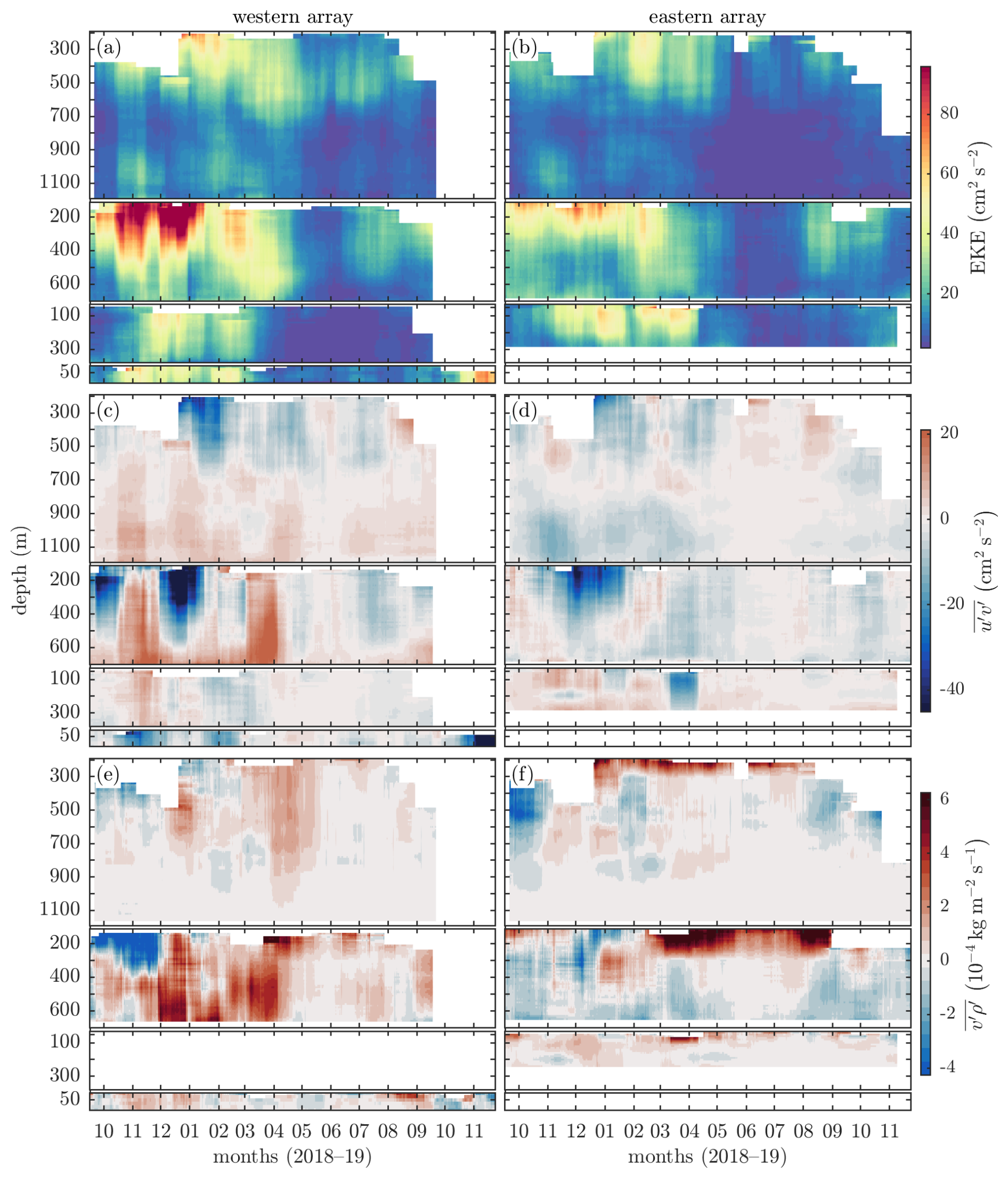
Figure A1 Time series of (a, b) EKE, (c, d) eddy momentum flux, (e, f) and eddy density flux, at the (left) western and (right) eastern arrays. In each panel (a–f), the moorings are ordered from the offshore (top) to onshore (bottom), e.g. W3, W2, W1, W0. The depth range at W0 was 30 to 80 m, and the vertical axis is scaled by a factor of 2 for clarity.

Appendix B: Model setup validation

B1 Validation against observations on the West Spitsbergen Shelf

The model setup used in this study was originally implemented by Frank et al. (2025) and validated against observations from Isfjorden and the West Spitsbergen Shelf obtained through the ocean observation program at the University Centre in Svalbard (Skogseth et al., 2020). Hydrographic and current measurements selected along a section across the West Spitsbergen Shelf and the WSC during three autumns were contemporary with the model simulations. At this section, the model had a systematic temperature bias, with colder surface waters and warmer deep water over the slope. Salinity was biased low, both in the surface layer and the AW layer. These compensating biases in temperature and salinity resulted in good agreement in density. The model realistically reproduced the circulation patterns in the region.

Temporal variability in the model simulations was validated against contemporaneous mooring records from the mouth of Isfjorden on the west coast of Svalbard. Simulated temperatures were generally slightly lower than observed but reproduced the temporal variability well. Simulated salinity and temperature were both slightly lower during winter, while agreement was good during the rest of the year. Density time series were well captured by the model. The inflow into Isfjorden was also well represented, with simulated current speeds in good agreement with the observations, although peak velocities were slightly overestimated.

B2 Model–observation comparison north of Svalbard

Because the model simulations were originally designed for the West Spitsbergen Shelf study by Frank et al. (2025), they do not overlap in time with the mooring observations used here. Nevertheless, we can compare the seasonal mean cross-slope structure of the boundary current and hydrography (Fig. B1).

The model bathymetry is based on IBCAO version 3 (Jakobsson et al., 2012), which is too shallow in the vicinity of the western mooring array. As a result, the steeper part of the slope is positioned farther offshore in the model relative to observations. To account for this, the virtual moorings were shifted offshore to align with comparable depths and slope characteristics as the in situ moorings (Sect. 3.3.3). Because the modelled bathymetry differs from the real bathymetry, direct comparisons of the full cross-slope sections are challenging. However, we can directly compare the hydrographic and current structure at the virtual moorings (Fig. B1) with those from the corresponding deeper mooring pairs (Fig. 2).

The simulated boundary current is located farther offshore and has a different seasonality than observed (Fig. B1). In September–February, the simulated current core, with 18 cm s⁻¹, is centred near the 1100 m isobath and extends from 100 to 1000 m depth at the western array (Fig. B1a). The observed current core during the same season reaches 20 cm s⁻¹, is located near the 700 m isobath at 100 m depth, and is weakening more rapidly with increasing depth (Fig. 2a). Both the simulated and observed currents in September–February strengthen downstream along-path from the western to the eastern array, reaching 23 cm s⁻¹ (Figs. B1b and 2b). In March–August, the simulated current is stronger, with maximum speeds increasing to 24 cm s⁻¹ at the western array and almost 30 cm s⁻¹ at the eastern array (Fig. B1c and d). This contrasts with the observations, which show a weakening of the current during this period (Fig. 2c and d).

The offshore displacement of the simulated velocity core relative to observations likely contributes to the lack of a clear seasonal signal in EKE and conversion rates in the model. It may also explain why the largest conversion rates occur offshore of the mooring arrays.

Both the observed and simulated temperature maxima were approximately 0.5 °C higher in September–February than in March–August (Figs. 2 and B1). However, the observed temperature maxima were approximately 0.5 °C higher than those in the model in both seasons. Despite being colder, the simulated water masses were also less dense. For example, the 1027.9 and 1028.0 kg m⁻³ isopycnals were located at depths of approximately 300–400 and 600–650 m in the observations, while in the model they were found deeper, near 600–650 and 1000 m respectively.

The virtual moorings and the 1400 m isobath selected for the analysis are positioned to capture both the simulated temperature core and the boundary current core.

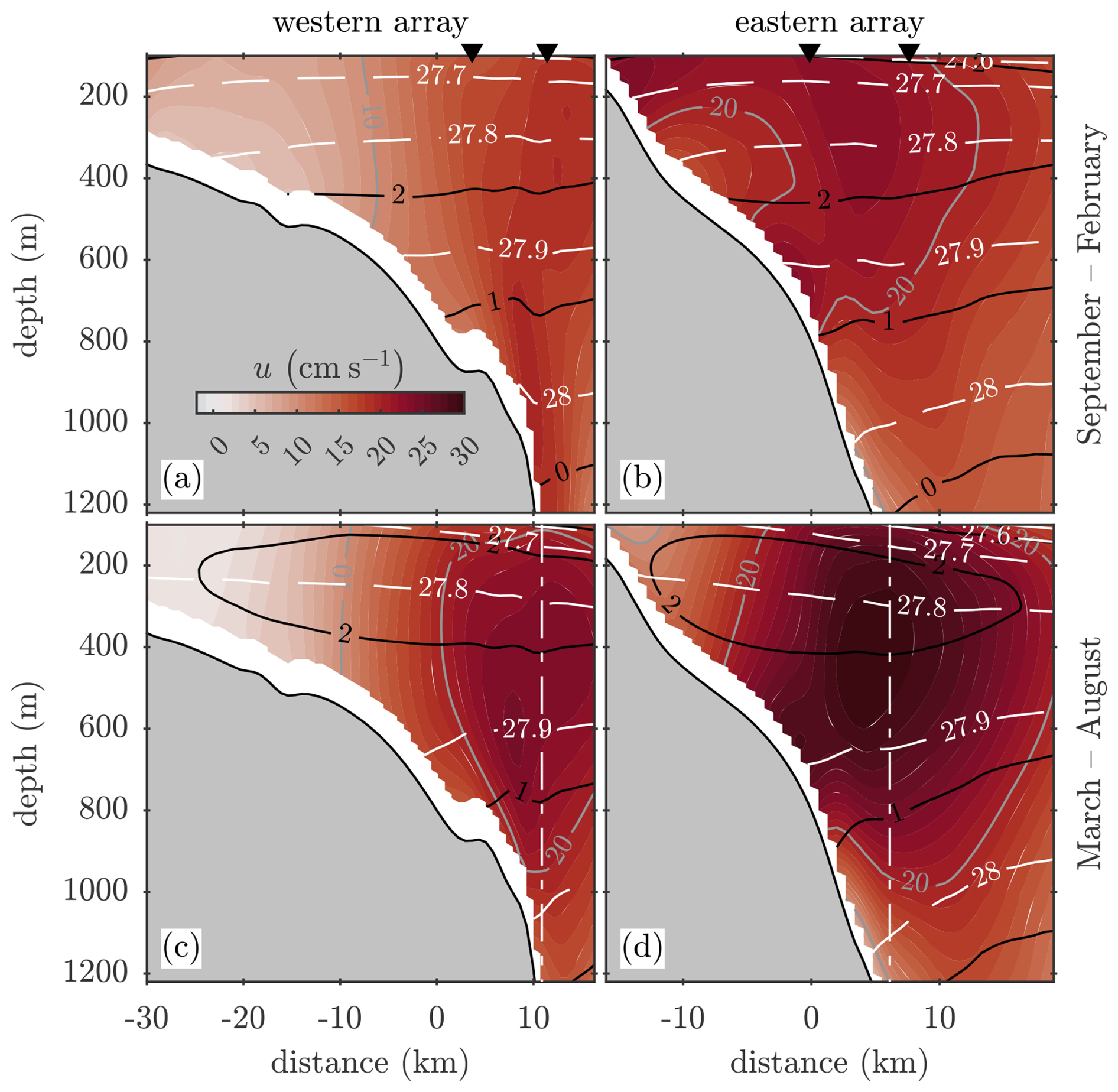
Figure B1 Average simulated along-slope current velocity u (colours) at (a, c) the western and (b, d) eastern mooring arrays during (a, b) autumn and winter (September–February) and (c, d) spring and summer (March–August) averaged over the two-year period. Grey contours show velocity every 10 cm s⁻¹, white dashed isopycnals every 0.1 kg m⁻³, and black isotherms every 1 °C. Triangles at the top mark the virtual mooring locations (a, b) and vertical white dash-dotted lines mark the location of the 1400 m isobath used in Sect. 3.3.2.

Appendix C: Passbands and filters for the eddy band

Various studies have used slightly different cutoff frequencies for the band-pass filter in their analyses. To illustrate the sensitivity to passband choice, we compare the original 35 h–14 d passband with a wider 48 h–30 d band used by von Appen et al. (2016) (Fig. C1). We also examine the effect of lowering the high-frequency cutoff toward 24 h, motivated by advective time scales ranging from 24 to 40 h. To approach a 24 h cutoff while avoiding contamination from the diurnal tidal band, we use a finite impulse response Kaiser filter, which provides a sharper transition between passband and stopband. The original 35 h–14 d passband using a Butterworth filter yields similar results to the Kaiser filter, with some minor differences at the longer time scales. The different filter choices are generally in good agreement, and our results are not strongly sensitive to the filter choices. The smallest difference is between the Butterworth and Kaiser filters when applied with the same passband. Time series with different passbands typically show similar magnitudes and variability, although the 48 h–30 d band occasionally deviates. The results are at times sensitive to the choice of high-frequency cutoff (27 h, 35 h, or 48 h). For example, in November 2018, BC shows the largest spread between passbands, as a result of differences in the fluctuations of v and ρ arising from the different cutoffs.

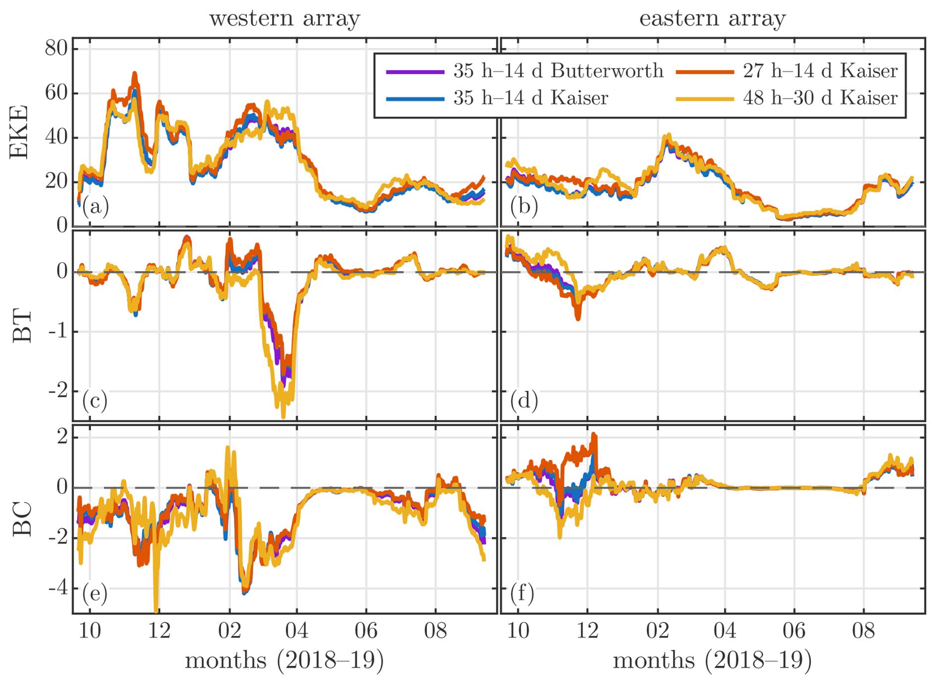
Figure C1 Example time series of EKE, BT, and BC at 460 m depth at the western (left) and eastern (right) mooring arrays showing the sensitivity to the choice of passband and filter type used in the band-pass filtering for fluctuation calculations.