TS-Cast: deep learning for subsurface ocean reconstruction from satellite observations in the northwestern Pacific

Since the 1990s, satellite observations have been providing reliable estimates of ocean surface state, including absolute dynamic topography (ADT), sea surface temperature (SST), and sea surface salinity (SSS) at sufficient space and time resolution to characterize ocean dynamics. Together with the extensive hydrographic dataset from Argo and ship-based hydrographic profiles, these measurements provide a comprehensive view of oceanic conditions. While ADT reflects full ocean dynamics, its steric component represents the integrated information for subsurface water properties. However, relating surface variables to subsurface profiles remains challenging because surface signatures are often non-linearly related to interior structures, and satellite data contain inherent non-steric signals. To address these limitations, we introduce TS-Cast, a novel uncertainty-aware deep neural network. Unlike direct regression models, TS-Cast is designed to adjust monthly climatological profiles as a physical prior and learns to dynamically adjust them. By using a 31 s sequence of satellite inputs (SST, SSS, and ADT) and quantifying prediction uncertainty, the model effectively captures the temporal variation of mesoscale dynamics. It was trained on approximately 155 000 Argo and ship-based thermohaline profiles in the northwestern Pacific. TS-Cast’s capability is demonstrated by comparisons with independent time-series data from moorings that measured temperature and salinity or vertical acoustic travel time. The network significantly improves upon the climatological baseline, achieving an overall Root Mean Square Error (RMSE) of <1° C for temperature and <0.1 psu for salinity in the upper 500 m depths at the Kuroshio Extension region. This performance is comparable to or surpasses that of data-assimilating numerical and statistical models, validating TS-Cast as a powerful tool for ocean monitoring. Critically, this framework reveals not only TS-Cast's high fidelity but also demonstrates that the limitations of the input satellite data fundamentally constrain its predictive skill.

1 Introduction

Ocean Temperature-Salinity (TS) vertical profiles are essential for understanding ocean circulation, heat content, climate change, and marine ecosystems (Talley, 2011). However, in-situ observations across the vast ocean are highly constrained by spatiotemporal sampling limitations. The Argo program has transformed our understanding of the ocean state, yet even this globally distributed TS profiling network maintains a density of roughly one float every 3° of latitude and longitude, providing new profiles only once every 10 d. While satellite remote sensing offers extensive spatial and temporal data coverage, it is inherently restricted to the ocean's surface. This data scarcity in the ocean's interior poses a significant challenge to fundamental oceanographic research, accurate climate-change assessments, and the development of ocean prediction and management strategies. This sparsity of subsurface observations limits our ability to fully resolve the ocean's 3-D dynamics.

Despite the surface limitations of satellite remote sensing, Sea Surface Height (SSH) measured by satellite altimetry contains depth-integrated information about the TS vertical structure. SSH is composed of the “steric part,” which arises from the thermal expansion and contraction of seawater due to temperature and salinity variations, and the “mass-loading part,” which is due to the actual accumulation of water (Park et al., 2012). Since the steric part accounts for the majority of SSH variations, SSH from satellite altimetry provides clues for estimating TS profiles. For this reason, various inverse methods have been and are continuously being developed to estimate TS from depth-integrated proxies without direct observation.

In the past and present, methods such as the Gravest Empirical Modes (GEM) technique were widely used. This approach involves creating a look-up table that relates proxies like acoustic travel time (τ) (Sun and Watts, 2001; Watts et al., 2001) or Absolute Dynamic Topography (ADT) (Meunier et al., 2022) to temperature and salinity profiles. While this method has achieved considerable success in specific regions, it assumes a time-invariant relationship, is regionally dependent, and has clear limitations in capturing complex, nonlinear dynamics that deviate from the historical mean state (Sun and Watts, 2001). To improve upon these linear statistical frameworks, efforts were made to blend satellite data with in-situ profiles through more sophisticated methods like multi-linear regressions combined with optimal interpolation (Guinehut et al., 2004, 2012).

To better capture the inherent nonlinearities, recent advances in machine learning combined with extensively accumulated oceanic data have led to the development of various profile estimation models. These approaches span a range of architectures, from relatively simple multi-layer perceptrons (MLPs) (Ali et al., 2004; Lu et al., 2019) to various forms of convolutional neural networks (CNNs) that excel at capturing spatial patterns (Sun et al., 2022; Smith et al., 2023; Song et al., 2024; Jiang et al., 2024; Lee et al., 2026), and recurrent neural networks (RNNs) like Long Short-Term Memory (LSTM) designed to capture sequential dependencies (Buongiorno Nardelli, 2020; Chen et al., 2023; Sammartino et al., 2025). These data-driven approaches are not limited to temperature and salinity, but have also been successfully applied to biogeochemical variables like chlorophyll-a and particulate backscattering coefficient (Sauzède et al., 2015, 2016). While validation against independent Argo profiles provides a robust assessment of spatial accuracy, these discrete profiles offer limited insight into continuous high-frequency variability. To complement this spatial validation, we introduce a rigorous temporal validation using continuous time-series observational data from moorings. This dual approach allows us to evaluate both the spatial structure and the capability to reproduce continuous, time-varying ocean dynamics.

This study presents a new AI-based TS profile reconstruction model, and a core contribution lies in a rigorous validation methodology. The objectives of this paper can be summarized as follows:

1. Develop and present a high-performance AI model that reconstructs Northwestern Pacific TS profiles from satellite surface data.

2. Assess the model's capability to reproduce continuous ocean dynamics by validating against multi-year, high-frequency timeseries mooring data, using spectral coherence analysis to quantify performance across different frequency bands.

3. Conduct an in-depth analysis of the physical causes of model error, demonstrating that its limitations are directly linked to the inherent characteristics and limitations of the input satellite altimetry data.

2 Data and Methods

2.1 Input and training data

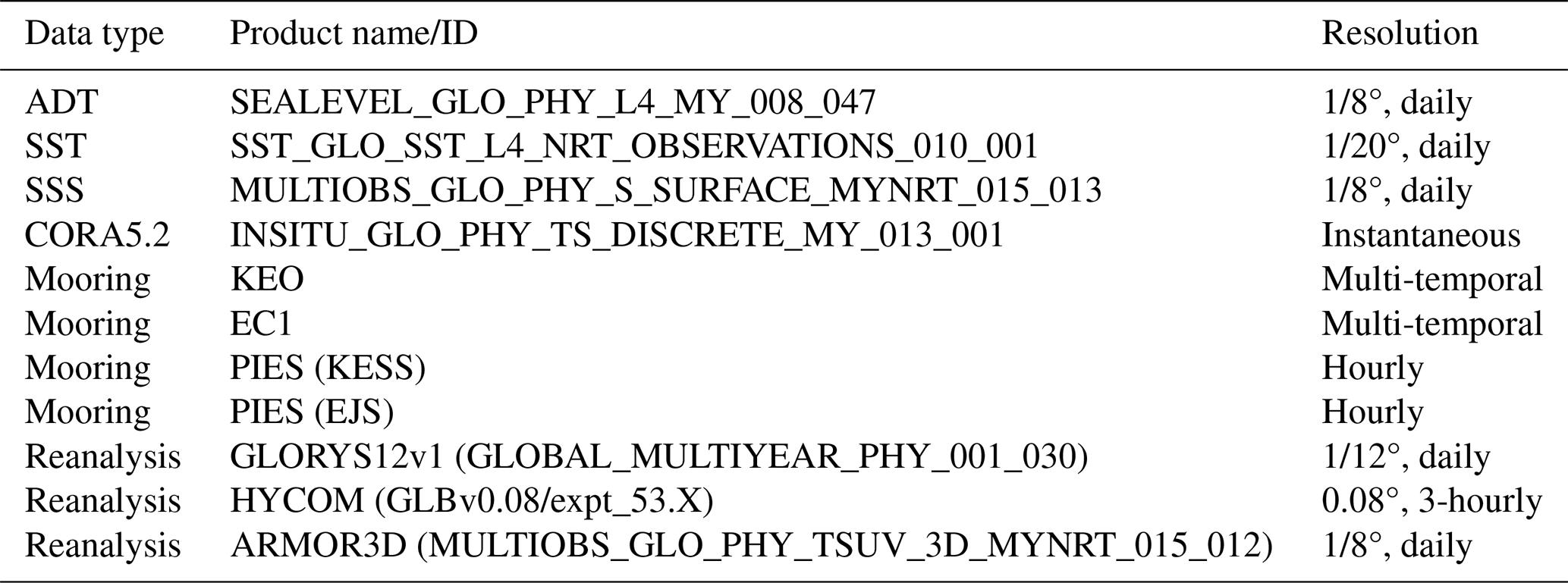
The input data for the AI model consist of gridded sea surface data derived from satellite observations. For this study, we focus on variables that directly describe the ocean's physical state. These variables, with daily temporal resolution from 1993 to 2023, include sea surface temperature (SST), sea surface salinity (SSS), and absolute dynamic topography (ADT). This approach intentionally excludes variables related to external atmospheric forcing (e.g., surface wind) or biogeochemical processes (e.g., ocean color). We used three daily products from the Copernicus Marine Service (CMEMS): Multi-mission ADT product at 1/8° spatial resolution (ID: SEALEVEL_GLO_PHY_L4_MY_008_047), OSTIA SST (Stark et al., 2007; Donlon et al., 2012; Good et al., 2020) at 1/20° spatial resolution (ID: SST_GLO_SST_L4_NRT_OBSERVATIONS_010_001), and the SSS (Droghei et al., 2016; Nardelli et al., 2016; Droghei et al., 2018; Sammartino et al., 2022) at 1/8° spatial resolution (ID: MULTIOBS_GLO_PHY_S_SURFACE_MYNRT_015_013). These products include error variables that represent the formal mapping error calculated via an optimal interpolation process. The variables indicate the uncertainty of the gridded field relative to the raw data along satellite tracks; however, they do not represent a complete error budget or include errors arising from physical processes (Le Traon et al., 1998). To unify the spatial resolution of the input data, all variables were regridded to a 1/8° grid resolution using linear interpolation. To encode geographic information and preserve the periodicity of the spherical domain, we transformed the coordinates into X, Y, and Z features (Sinha and Abernathey, 2021):

$$\begin{array}{}\text{(1)}& \left[\begin{array}{c}X\\ Y\\ Z\end{array}\right]=\left[\begin{array}{c}\sin (\mathit{\varphi }\times \frac{\mathit{\pi }}{\mathrm{180}})\\ \sin (\mathit{\lambda }\times \frac{\mathit{\pi }}{\mathrm{180}})\cdot \cos (\mathit{\varphi }\times \frac{\mathit{\pi }}{\mathrm{180}})\\ -\cos (\mathit{\lambda }\times \frac{\mathit{\pi }}{\mathrm{180}})\cdot \cos (\mathit{\varphi }\times \frac{\mathit{\pi }}{\mathrm{180}})\end{array}\right]\end{array}$$

where ϕ is latitude and λ is longitude. These X, Y and Z features were used as the model input.

For the training dataset, thermohaline profiles from CTD and Argo floats were sourced from the Coriolis Ocean dataset for Reanalysis version 5.2 (CORA5) Easy CORA product provided by CMEMS (ID: INSITU_GLO_PHY_TS_DISCRETE_MY_013_001). This is a delayed-mode dataset with preprocessed and quality-controlled profiles from CTD, Argo floats, and other platforms. The profiles are separated into training set (1993–2020) and test set (2021–2023). We selected profiles that reached a maximum pressure greater than 700 dbar for the training process. This resulted in a training set of 155 030 profiles distributed across the study area (Fig. 1). For monthly climatological thermohaline profiles, we used the World Ocean Atlas 2023 (WOA23) dataset, which has a 1/4° spatial resolution (Reagan et al., 2023) and it was linearly interpolated into 1/8° resolution. All in-situ and climatological profiles were linearly interpolated onto 128 evenly spaced vertical layers between 10 and 700 dbar. In-situ profiles from regions where WOA23 climatological profiles extended to at least 700 dbar were included in both training and test datasets. Only profiles containing more than 50 valid observation points within the sampled depth range (typically 10–1500 dbar) were used. For these profiles, linear interpolation was applied as a vertical resampling step to align the data onto the 128 vertical levels. Profiles with gaps were excluded from training. For the test dataset, profiles with gaps were retained by applying masks to use only valid-level observations for error estimation.

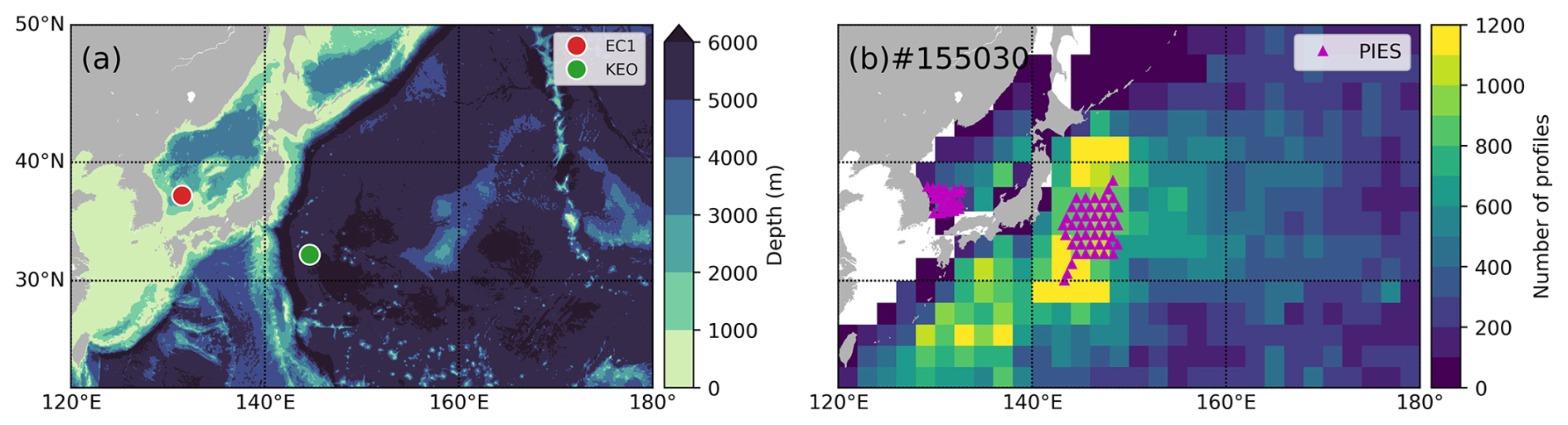
Figure 1 The study area and locations of the in-situ observation data used. (a) Bathymetry of the study region and the locations of the key time series mooring sites, EC1 (red circle) and KEO (green circle). (b) Spatial distribution of the temperature and salinity profiles used in the training set and the locations of the PIES arrays (triangles).

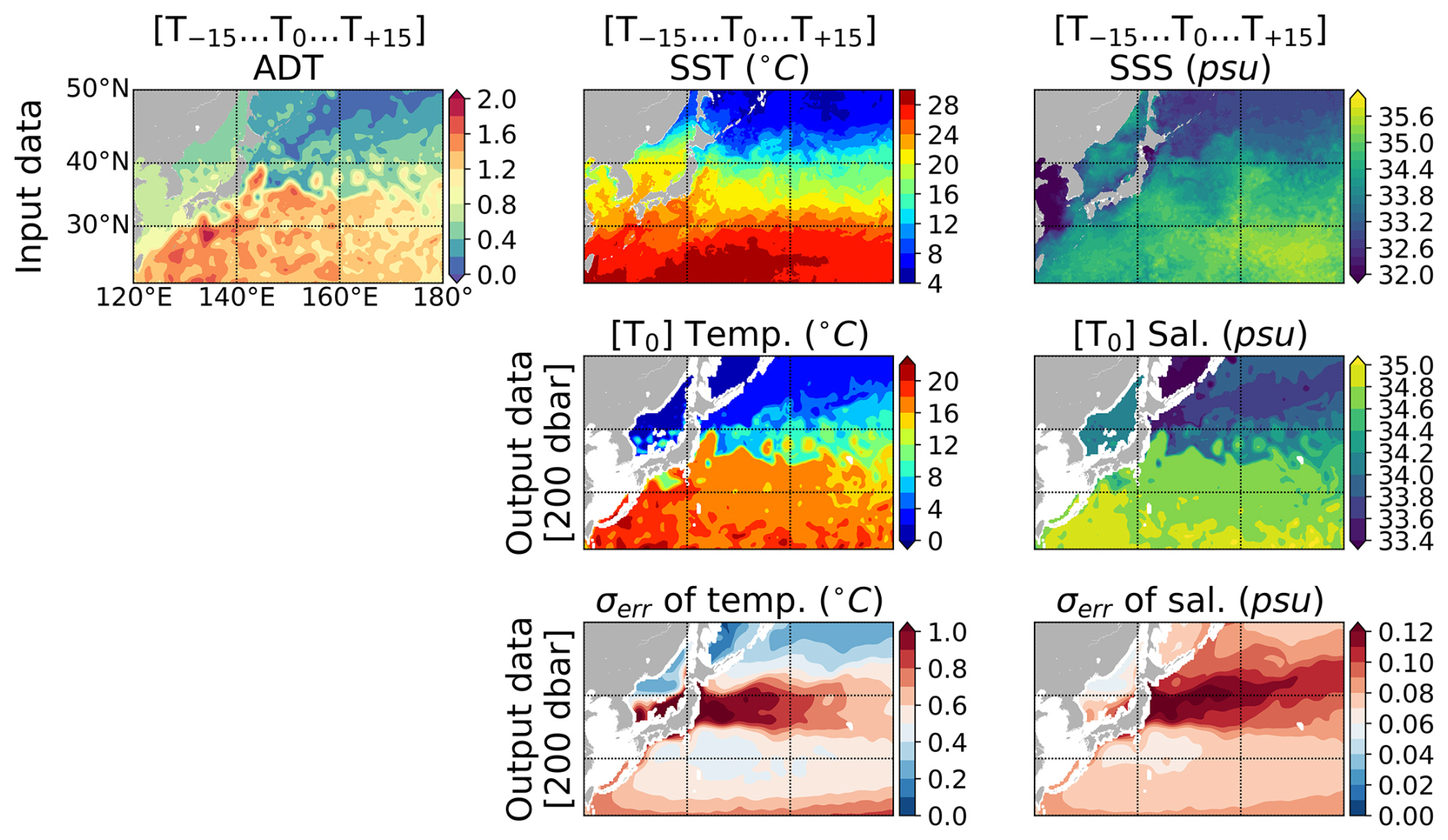
Figure 2 An example of the input data and spatially concatenated output profiles for the TS-Cast model. (Top panels) Model input data with ±15 d window centered on a specific time (T₀): Absolute Dynamic Topography (ADT), Sea Surface Temperature (SST), and Sea Surface Salinity (SSS). (Middle panels) Temperature and Salinity at 200 dbar depth, estimated by the TS-Cast model at time T₀. (Bottom panels) The standard deviation of the error (σ_Err) for the temperature and salinity estimates, also predicted by the model for the same time and depth.

2.2 Validation data

Our validation involved a two-step procedure: basin-scale and core validation.

The first step, basin-scale validation, assessed the overall performance throughout the study area by a 10° meridional interval. For this, we used the number of 23 631 profiles from the test set (2021–2023).

The second step, core validation, focused on evaluating the model's long-term temporal consistency using continuous time series data from mooring observations. For this purpose, we used data from the Kuroshio Extension Observatory (KEO), the East/Japan Sea (EJS) Current Measurements (EC1) mooring, and two Pressure-Inverted Echo Sounder (PIES) arrays. The KEO buoy was deployed in the Kuroshio Extension recirculation gyre (32.3° N, 144.6° E) and has measured TS at 32 depths down to 525 m since June 2004. The EC1 mooring (Noh and Nam, 2018) is located in the Ulleung Interplain Gap (UIG) of the EJS and is equipped with sensors at multiple depths (e.g., 400, 1400, 2200 m). For the EC1 mooring data, only temperature data are compared due to the lack of salinity observations. The analysis focused on the 2006–2012 period, as the observations were concentrated in the thermocline. Both KEO and EC1 moorings are part of the OceanSITES network. Since OceanSITES data are routinely assimilated into ocean reanalysis models, these moorings do not provide independent observations for validation. On the other hand, data from the PIES array are not assimilated into ocean reanalysis products, providing independent observations for validation. We used two PIES arrays. One, an array of 46 instruments was deployed during the KESS project (2004–2006), and the other, an array of 25 PIES deployed in the EJS, covering the Ulleung Basin from 1999–2001. As a broader performance benchmark, we also compared our results with temperature and salinity outputs from the HYCOM, GLORYS, and ARMOR3D reanalysis products for the period from 1994 to 2015 (Table 1). This period corresponds to the available period of the HYCOM reanalysis outputs. While all three are data-assimilative products, HYCOM and GLORYS are based on numerical ocean models, whereas ARMOR3D (Guinehut et al., 2012) is a statistically-based product. To ensure temporal consistency, all mooring and model outputs used in the validation step were averaged to daily resolution.

To evaluate the spectral dependence of the model's performance, we computed the magnitude squared coherence between the observed and estimated time series. The coherence estimates were obtained using Welch's method with a Hanning window of 128 d and 50 % overlap. The 95 % significance level for the coherence estimates was determined based on the degrees of freedom (Thomson and Emery, 2014).

Table 1 Summary of the datasets used in this study.

2.3 Thermohaline profile estimating network (TS-Cast)

Our proposed model, the thermohaline profile estimating network (TS-Cast), is designed to estimate vertical thermohaline profiles by dynamically adjusting monthly climatological profiles using satellite-measured sea surface data (Fig. 2). TS-Cast's key innovation lies in its hybrid approach. Rather than generating profiles solely from instantaneous satellite data, it treats the monthly climatological profile as a physically-grounded prior and learns its dynamic adjustments from real-time satellite observations. This conditioning is performed within a U-Net architecture (Çiçek et al., 2016) by leveraging Feature-wise Linear Modulation (FiLM) layers (Perez et al., 2018). The architecture consists of four components: (i) a satellite feature encoder, (ii) a U-Net backbone operating on the climatological prior, (iii) FiLM conditioning layers that inject satellite information into the U-Net, and (iv) parallel output heads for the temperature/salinity prediction and the error variance. Each component is described below.

2.3.1 Satellite feature encoder

The satellite feature encoder (Fig. 3a) compresses spatiotemporal satellite observations into a single latent vector h∈ℝ⁵¹² that conditions the U-Net. The encoder takes two inputs. The first is a spatiotemporal tensor of shape [6, 31, 15, 15] corresponding to [channels, series, latitude, longitude]. The six channels comprise SST, SSS, ADT, and their respective error fields over a 31 d sequence within a $\sim \mathrm{2}\mathit{°}\times \mathrm{2}\mathit{°}$ (15×15 grid) window centered on the target location. The 2° radius is chosen to contain an entire mesoscale eddy (typically 100–300 km) (Chelton et al., 2011), and the 31 d window (±15 d) captures the dynamic evolution of eddies on timescales of tens of days to months. Geographic coordinates encoded as [$X,Y,Z$] features (Sect. 2.1), with shape [3, 1, 15, 15], are concatenated along the channel dimension. This tensor is processed by a sequence of 3D residual convolutional blocks (each consisting of 3D convolution, Mish activation (Misra, 2019), and average pooling), progressively reducing the spatial and temporal dimensions to produce a [512, 1, 1, 1] feature vector.

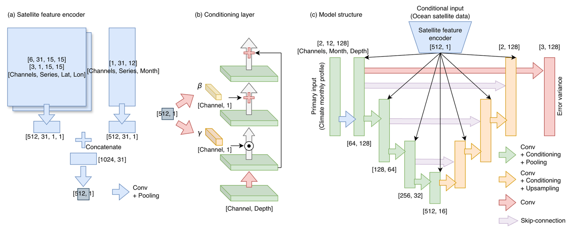
Figure 3 Schematic diagram of the TS-Cast model architecture. (a) The satellite feature encoder architecture. It takes two inputs. The first is a tensor of satellite-derived data with a shape of [6, 31, 15, 15] and encoded geographic information (X, Y, and Z) with a shape of [3, 1, 15, 15] corresponding to [Channels, Series, Latitude, Longitude]. The 6 channels include SST, SSS, ADT, and their respective error fields over a 31 d sequence. The second input, with a shape of [1, 31, 12], provides sea level anomaly information, representing the difference between the 31 d ADT and the 12 climatological monthly dynamic heights. (b) The architecture of the conditioning layer. The scaling (γ) and shifting (β) parameters to modulate the feature maps are generated by the encoded context vector. (c) The overall U-Net-based model architecture. The primary input is a climate monthly profile, and the conditioning information from the satellite feature encoder is injected into each layer.

The second input characterizes the current dynamical state relative to the climatological seasonal cycle. It consists of a vector of shape [1, 31, 12], computed as the difference between the 31 d ADT sequence and the 12 monthly climatological dynamic heights at the profile location. This provides a baseline for the steric signal across the full seasonal cycle, allowing the network to contextualize eddy- or front-induced deviations relative to the expected annual variability. The dynamic height (DH) is computed as $\mathrm{DH}=\frac{\mathrm{1}}{g}{\int }_{P_{\mathrm{ref}}}^{P_{\mathrm{0}}}\mathit{\alpha }dp$, where α is the specific volume anomaly and the reference pressure P_ref is set at 700 dbar. The 12-month climatological comparison provides the seasonal cycle context that complements the satellite inputs. This vector is processed by 2D residual convolutional blocks (2D convolution, Mish activation, and average pooling) to produce a [512, 1] vector. The two resulting vectors are concatenated to form a [1024, 1] tensor, which is passed through a final convolutional block to produce the latent vector h.

2.3.2 U-Net backbone

The U-Net backbone (Fig. 3c) takes monthly climatological thermohaline profiles from the WOA23 as input at a spatial point. These profiles are interpolated into 128 evenly spaced vertical layers between 10 and 700 dbar (e.g., $\mathrm{12}\times \mathrm{128}\times \mathrm{2}$ for months, levels, and TS channels). The number of layers was set to 128 (2⁷) to achieve a vertical resolution of approximately 5 dbar, with a format well-suited for the U-Net's encoding-decoding process. An initial 2D residual convolutional block with a kernel spanning all 12 months collapses the temporal axis (mathematically equivalent to a 1D convolution with 12×2 channels) producing a 1D tensor of shape [64, 128] that represents the integrated annual climatological context.

The resulting tensor is processed by a symmetric encoder–decoder structure using 1D residual convolution blocks. The encoder consists of four down-sampling blocks (1D residual convolution block + FiLM conditioning + average pooling with stride 2), reducing the vertical dimension from 128 to 16 while increasing the channel dimension from 64 to 512. The decoder mirrors this structure with four up-sampling blocks (1D residual convolution block + FiLM conditioning + linear upsampling), restoring the vertical dimension to 128. Skip connections concatenate matching encoder and decoder feature maps at each level, preserving fine-scale vertical structure. FiLM conditioning is applied at every encoder and decoder block, injecting the satellite-derived information from h into the network at multiple scales.

2.3.3 FiLM conditioning

FiLM layers inject the latent vector h into the U-Net at each encoding and decoding step. At each encoding and decoding step i, a FiLM layer modulates the intermediate feature map x_i. Let x_i be a tensor with C_i feature channels. For our 1D profile data, $x_i\in {\mathbb{R}}^{L_i\times C_i}$, where L_i is the length of the profile (e.g., number of pressure levels). The FiLM layer applies a channel-wise affine transformation using parameters derived from the encoded satellite data. This operation is defined for each channel c (where $\mathrm{1}\le c\le C_i$) as:

$$\begin{array}{}\text{(2)}& \text{FiLM}(x_i{)}_c={\mathit{\gamma }}_{i,c}\cdot x_{i,c}+{\mathit{\beta }}_{i,c}\end{array}$$

Here, x_i,c represents the cth feature map (channel) of x_i. The scaling factor γ_i,c and the shifting factor β_i,c are the components of two vectors, ${\mathit{\gamma }}_i\in {\mathbb{R}}^{C_i}$ and ${\mathit{\beta }}_i\in {\mathbb{R}}^{C_i}$. These vectors are generated by a dedicated conditioning network g_i from a shared latent vector h. The conditioning network g_i is implemented as a multi-layer perceptron (MLP) with two residual blocks (He et al., 2016). To align the modulation capacity with the feature representation at each step, the number of hidden units is set to match the channel dimension C_i, ranging from 64 to 512. This network maps the 512-dimensional latent vector h to the required 2×C_i parameters.

2.3.4 Output heads

The U-Net produces two parallel outputs. The first output head predicts the temperature and salinity profiles ($\widehat{T},\widehat{S}$), producing a tensor of shape [2, 128]. The second output head predicts the depth-dependent logarithmic error variances ($\log {\widehat{\mathit{\sigma }}}_T^{\mathrm{2}},\log {\widehat{\mathit{\sigma }}}_S^{\mathrm{2}},\log {\widehat{\mathit{\sigma }}}_{\mathit{\rho }}^{\mathrm{2}}$), producing a tensor of shape [3, 128], from the input monthly climatological profiles to capture seasonal and depth-dependent uncertainty. The first head uses all intermediate feature representations of the U-Net. We chose to predict the density variance ${\widehat{\mathit{\sigma }}}_{\mathit{\rho }}^{\mathrm{2}}$ independently rather than deriving it from ${\widehat{\mathit{\sigma }}}_T^{\mathrm{2}}$ and ${\widehat{\mathit{\sigma }}}_S^{\mathrm{2}}$ because the covariance between T and S errors in the ocean is non-negligible and cannot be ignored in error propagation. Furthermore, the $\frac{\mathrm{1}}{\mathrm{2}}\log {\widehat{\mathit{\sigma }}}^{\mathrm{2}}$ regularization term in the loss (Sect. 2.4) penalizes variance inflation, preventing the network from trivially increasing ${\widehat{\mathit{\sigma }}}_{\mathit{\rho }}^{\mathrm{2}}$ to avoid the density consistency penalty.

2.3.5 Training

We trained the network for 250 epochs using the AdamW optimizer (Loshchilov and Hutter, 2017) with an initial learning rate $\mathrm{1}\times {\mathrm{10}}^{-\mathrm{5}}$ and a batch size of 512. Twenty percent of training data were reserved for validation. To obtain robust and stable estimates, the final thermohaline profile was calculated as the ensemble mean of the outputs from the three independently trained networks initialized with different random seeds.

2.4 Physical Constraints and Uncertainty-Aware Loss

To ensure physical consistency in the model's estimations, we incorporated two key strategies into our loss function: a density-based physical constraint and an uncertainty-aware weighting scheme. TS-Cast network directly estimates temperature ($\widehat{T}$) and salinity ($\widehat{S}$) profiles, but also their associated depth-dependent uncertainty via the predicted error variance (σ²). Instead of predicting the variance directly, the network outputs the logarithmic error variance (log σ²) to ensure numerical stability. This approach, based on the work of multi-task learning using uncertainty (Kendall et al., 2018), allows the model to learn spatiotemporal and depthwise varying error variances, effectively giving less weight to predictions in regions or depths with naturally high variability. The loss for temperature and salinity is formulated to minimize the negative Gaussian log-likelihood, which results in the following expression for each vertical level (i):

$$\begin{array}{}\text{(3)}& {\displaystyle }{\mathcal{L}}_T={\displaystyle \frac{\mathrm{1}}{N}}\sum _{i=\mathrm{1}}^N\left({\displaystyle \frac{\mathrm{1}}{\mathrm{2}{\widehat{\mathit{\sigma }}}_{T,i}^{\mathrm{2}}}}(T_i-{\widehat{T}}_i{)}^{\mathrm{2}}+{\displaystyle \frac{\mathrm{1}}{\mathrm{2}}}\log {\widehat{\mathit{\sigma }}}_{T,i}^{\mathrm{2}}\right)\text{(4)}& {\displaystyle }{\mathcal{L}}_S={\displaystyle \frac{\mathrm{1}}{N}}\sum _{i=\mathrm{1}}^N\left({\displaystyle \frac{\mathrm{1}}{\mathrm{2}{\widehat{\mathit{\sigma }}}_{S,i}^{\mathrm{2}}}}(S_i-{\widehat{S}}_i{)}^{\mathrm{2}}+{\displaystyle \frac{\mathrm{1}}{\mathrm{2}}}\log {\widehat{\mathit{\sigma }}}_{S,i}^{\mathrm{2}}\right)\end{array}$$

Here, (T_i,S_i) are the ground-truth values, ($\widehat{T_i},{\widehat{S}}_i$) are the model predictions, and (${\widehat{\mathit{\sigma }}}_T^{\mathrm{2}},{\widehat{\mathit{\sigma }}}_S^{\mathrm{2}}$) are the predicted error variances for temperature and salinity, respectively. This formulation encourages the model to produce smaller errors where its estimated error variance (${\widehat{\mathit{\sigma }}}^{\mathrm{2}}$) is low and allows for larger deviations where the error variance is high. The $\frac{\mathrm{1}}{\mathrm{2}}\log {\widehat{\mathit{\sigma }}}^{\mathrm{2}}$ term prevents the network from trivially inflating the variance to evade the consistency penalty. Notably, this uncertainty-weighted loss acts as an adaptive normalization mechanism, allowing the model to handle the different scales of temperature, salinity, and density without requiring explicit pre-standardization of the target variables. The model learns to predict this error variance by using the local monthly climatology profile as input, which provides essential information about regional variability and seasonal water mass characteristics.

In addition to the prediction accuracy of TS profiles, we enforce a physical constraint based on the equation of state for seawater (Fofonoff and Millard, 1983), adopting the physics-informed approach (Sammartino et al., 2025). While the network does not directly output density, we compute the density profile ($\widehat{\mathit{\rho }}$) from the predicted TS profiles ($\widehat{T},\widehat{S}$) and compare it to the ground-truth density (ρ) derived from the label profiles (T,S). This term penalizes the model for generating physically implausible combinations of temperature and salinity.

$$\begin{array}{}\text{(5)}& {\mathcal{L}}_{\mathit{\rho }}={\displaystyle \frac{\mathrm{1}}{N}}\sum _{i=\mathrm{1}}^N\left({\displaystyle \frac{\mathrm{1}}{\mathrm{2}{\widehat{\mathit{\sigma }}}_{\mathit{\rho },i}^{\mathrm{2}}}}({\mathit{\rho }}_i-{\widehat{\mathit{\rho }}}_i{)}^{\mathrm{2}}+{\displaystyle \frac{\mathrm{1}}{\mathrm{2}}}\log {\widehat{\mathit{\sigma }}}_{\mathit{\rho },i}^{\mathrm{2}}\right)\end{array}$$

where ${\widehat{\mathit{\sigma }}}_{\mathit{\rho }}^{\mathrm{2}}$ is the predicted error variance for density. The final composite loss function for training is a sum of these individual components:

$$\begin{array}{}\text{(6)}& {\mathcal{L}}_{\text{total}}={\mathcal{L}}_T+{\mathcal{L}}_S+{\mathcal{L}}_{\mathit{\rho }}\end{array}$$

This formulation addresses the weighting among the different error terms. Instead of using fixed hyperparameters, the model learns the optimal, data-dependent weight for each observation through the predicted variance σ². This multi-objective loss function guides the model to produce results that are not only accurate but also physically consistent.

3 Results

3.1 Basin-scale validation using CTD and ARGO profiles

The overall performance of the TS-Cast model was first evaluated against a test set of scattered CTD/ARGO profiles across the Northwestern Pacific. Figure 4 shows the vertical profiles of the root mean square error (RMSE) for both temperature and salinity, binned into six distinct latitudinal bands between 20° N and 50° N. The evaluation also includes a specific regional validation for the EJS, shown as blue and green lines for latitudes north of 35° N.

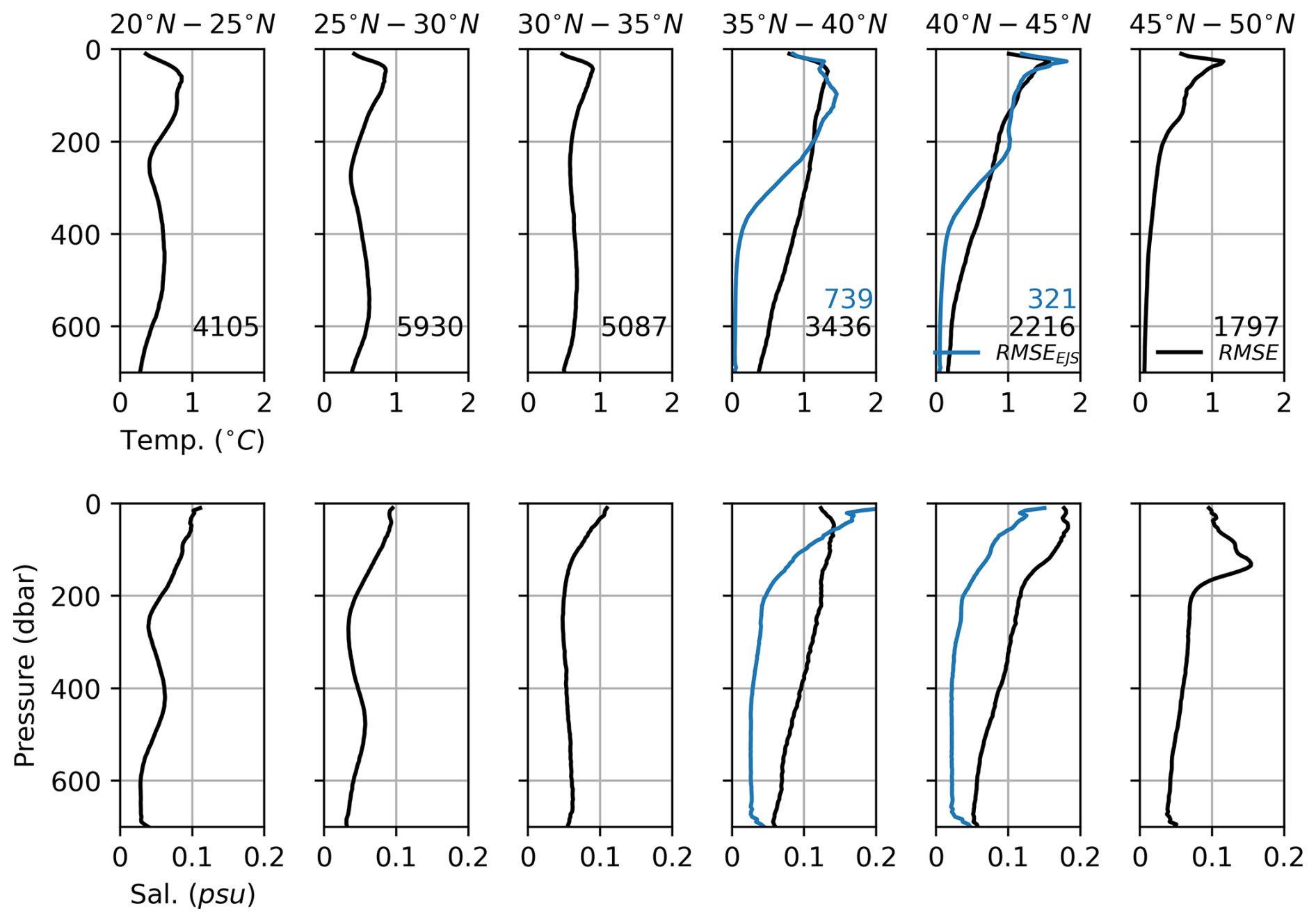
Figure 4 Vertical profiles of Root Mean Square Error (RMSE) for the test set. The results are binned into six latitudinal bands (columns) for temperature (top row) and salinity (bottom row). In each panel, the solid lines are the RMSE for the entire basin within that band. For latitudes north of 35° N, performance in the East/Japan Sea is shown separately with a blue line. The numbers indicate the count of profiles used for validation in each region.

For temperature, the RMSE across the wider Northwestern Pacific (black line) is generally below 1.0° C but shows a clear latitudinal trend. In the southern bands (20° N–35° N), the RMSE is consistently low (≤1° C), while performance degrades in the northern bands (40° N–45° N), with the RMSE peaking at nearly 2° C. This subsurface maximum corresponds to the main thermocline. In sharp contrast, below 300 dbar, the model shows high accuracy for the EJS (blue line). The RMSE in the EJS remains close to 1° C or lower than 2° C, comparable to the basin-scale results. This suggests the model effectively captures the unique and relatively uniform thermal structure of the EJS.

For salinity, the basin-scale RMSE (black line) also increases with latitude, rising from 0.1 psu in the south to nearly 0.2 psu in the north. The largest errors are in the upper 200 dbar. Again, the model's performance in the EJS (blue line) shows a different pattern. The salinity RMSE for the EJS is consistently lower than in the open Pacific, generally staying below 0.1 psu. This highlights the model's capability in handling the distinct water mass properties of this semi-enclosed marginal sea.

To assess the contribution of the climatological information to TS-Cast, we conducted an ablation experiment in which the climatological profile prior and the ADT anomaly vector were replaced with zeros, hereafter referred to as TS-Cast (no clim.). The results (Fig. 5) show that removing the climatological inputs has minimal impact on the basin-scale RMSE, with the climatological prior providing only modest gains in final prediction accuracy. However, the training dynamics reveal a clear difference. The TS-Cast model exhibits substantially more stable validation loss compared with TS-Cast (no clim.), which shows large fluctuations throughout training. We therefore retain the climatological input as a physically meaningful architectural component that stabilizes learning, while being transparent about its limited contribution to prediction accuracy.

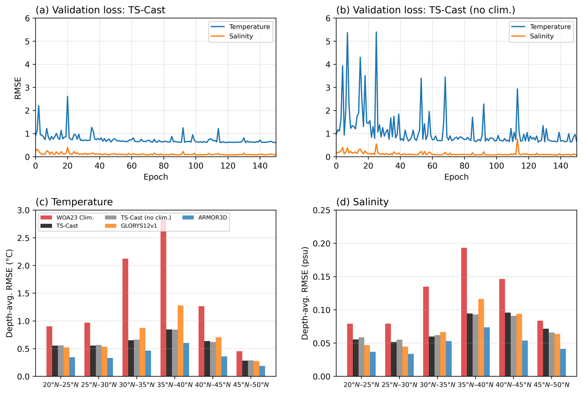
Figure 5 Root Mean Square Error (RMSE) for temperature and salinity for the validation set during the training process regarding (a) TS-Cast and (b) TS-Cast without climatological information. Depth-averaged RMSE for the test set regarding (c) temperature and (d) salinity. The results are binned into six latitudinal bands.

To address concerns regarding the independence of our validation, we benchmarked TS-Cast against GLORYS12v1, ARMOR3D, and the WOA23 monthly climatology on the test set. HYCOM is excluded from the basin-scale comparison because its reanalysis output does not extend to the 2021–2023 test period. We note that this comparison inherently favors the reanalysis products, as both GLORYS12v1 and ARMOR3D assimilate in-situ profiles from the CORA dataset, which includes the Argo and CTD profiles used for evaluation. Despite this disadvantage, TS-Cast achieves performance comparable to GLORYS12v1 across all latitude bands for both temperature and salinity, and substantially outperforms the WOA23 climatological baseline (Fig. 5). ARMOR3D exhibits the lowest RMSE overall, consistent with its direct assimilation of the evaluation data.

These results demonstrate that the TS-Cast model can produce physically realistic and accurate TS profiles. The comparative analysis reveals a nuanced picture of its performance: while the model provides a strong baseline for the entire basin, its accuracy is highest in the subtropical regions and within the geographically distinct EJS. The model's performance is somewhat lower in the highly variable subarctic frontal zones of the open Pacific, highlighting the challenge of modeling these complex regions.

3.2 Validation against In-Situ Mooring Observations

TS-Cast performance was validated against long-term mooring observations from two contrasting regions: the KEO station (Kuroshio Extension) and EC1 station (EJS). Validation context differs by product type. The reanalysis products (GLORYS, HYCOM, and ARMOR3D) assimilate OceanSITES mooring data (Cummings, 2005; Tanguy et al., 2025; Guinehut et al., 2012). Their agreement with these moorings reflects self-consistency of the data assimilation rather than independent skill. TS-Cast was trained exclusively on satellite surface data and sparse ARGO/CTD profiles, so it was not exposed to any subsurface mooring observations. Therefore, this comparison tests its genuine generalization capability to infer vertical structure from surface patterns.

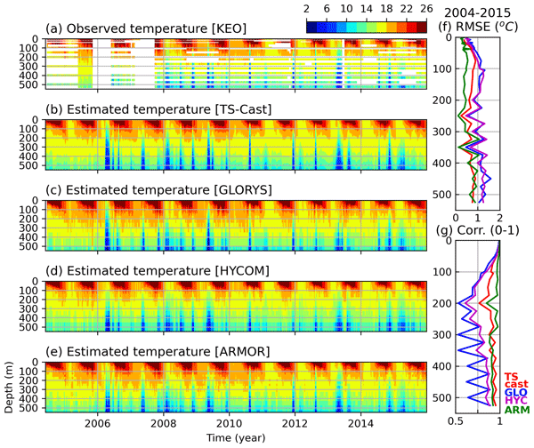
The KEO mooring has provided continuous multi-year observations since 2004 in the energetic Kuroshio Extension, a region characterized by intense mesoscale eddy activity. The reconstructed TS-Cast temperature field (Fig. 6b) demonstrates high fidelity to observations (Fig. 6a), successfully infilling significant temporal gaps while robustly capturing both the pronounced seasonal cycle in the upper ocean and the deeper, irregular isotherm displacements driven by eddy or meandering processes.

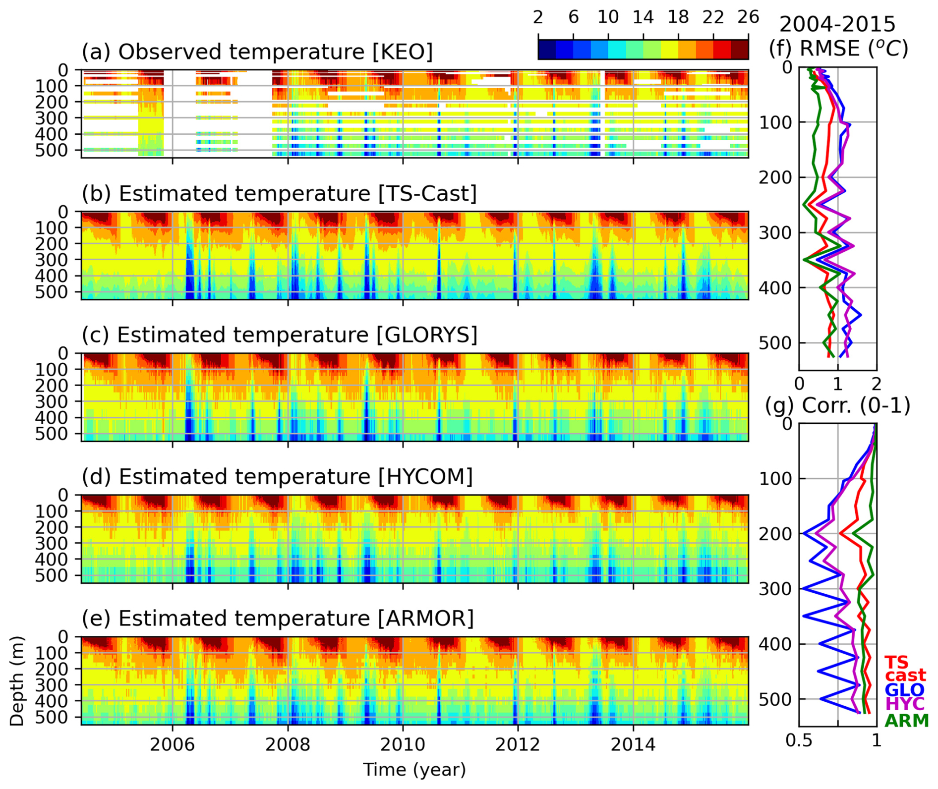
Figure 6 Time series comparison of observed and estimated temperature at the KEO site from 6/2004 to 12/2015. (a) Temperature observed at the KEO mooring. Temperature estimated by (b) TS-Cast, (c) GLORYS, (d) HYCOM, and (e) ARMOR3D. (f) Root Mean Square Error (RMSE) and (g) correlation coefficient with depth. The red line indicates the performance of TS-Cast. GLORYS, HYCOM, and ARMOR3D shown in blue, magenta, and green, respectively.

Quantitative validation metrics (Fig. 6f, g) confirm this visual assessment. In the upper 300 m, where seasonal variability dominates, TS-Cast achieves lower RMSE and higher correlation outperforming both GLORYS and HYCOM reanalyses. ARMOR3D exhibits the highest overall performance (r>0.85 at all depths), consistent with its direct assimilation of KEO mooring data. Notably, TS-Cast performance converges with ARMOR3D below 300 m depth (both r≈0.9), demonstrating that satellite surface observations alone can achieve subsurface reconstruction skill comparable to in-situ assimilative products in the main thermocline.

TS-Cast demonstrates similarly strong performance for salinity (Fig. 7). Correlation coefficients (Fig. 7g) remain significantly higher than GLORYS and HYCOM reanalyses down to 500 m layer, indicating accurate capture of subsurface salinity variability in both phase and amplitude, properties that challenge numerical ocean models. The consistently lower RMSE between 300 and 500 m (Fig. 7f) further demonstrates enhanced skill in representing the complex vertical haline structure of the Kuroshio Extension. Below 300 m depth, TS-Cast achieves correlation (r≈0.9) outperforming ARMOR3D, demonstrating that satellite surface observations can effectively constrain main halocline properties. Additionally, qualitative differences are reflected in reconstruction characteristics by exhibiting vertical discontinuities, particularly evident between 100–300 m depth, which appear to be artifacts in ARMOR3D fields (Fig. 7e).

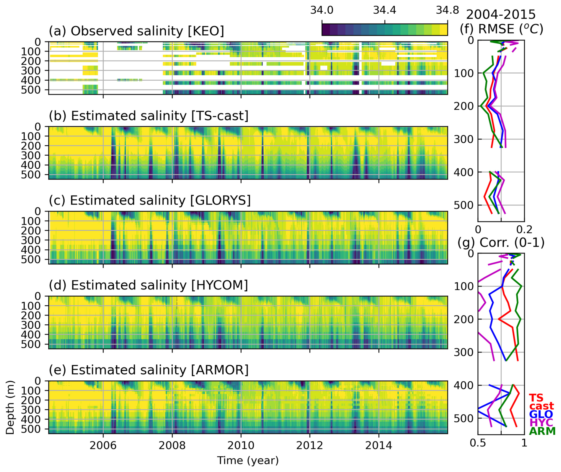
Figure 7 Time series comparison of observed and estimated salinity at the KEO site from 6/2004 to 12/2015. (a) Salinity observed at the KEO mooring. Salinity estimated by (b) TS-Cast, (c) GLORYS, (d) HYCOM, and (e) ARMOR3D. (f) Root Mean Square Error (RMSE) and (g) correlation coefficient with depth. The red line indicates the performance of TS-Cast. GLORYS ,HYCOM, and ARMOR3D shown in blue, magenta, and green, respectively.

Validation at the EC1 mooring (Fig. 8) serves as a strict test of the model's generalization ability in a different physical environment under conditions of data sparsity. TS-Cast successfully reconstructs the dominant oceanographic features of the EJS, including the deep vertical mixing in winter that forms thick mixed layers and the strong, shallow stratification in summer (Fig. 8b). The discrete performance metrics (Fig. 8f, g), plotted as scatter points due to the data gaps, reveal a consistent trend. TS-Cast (red triangles) exhibits generally lower RMSE and higher correlation values across the water column than the reanalysis products. There was no significant difference between RMSE (depth-mean RMSE ∼1.6° C), but the HYCOM and GLORYS show lower correlation (∼0.2) than TS-Cast and ARMOR3D (∼0.6). This reconstruction from limited data demonstrates the model's robustness and its capability to infer realistic subsurface structures, confirming its applicability across diverse circulation regimes.

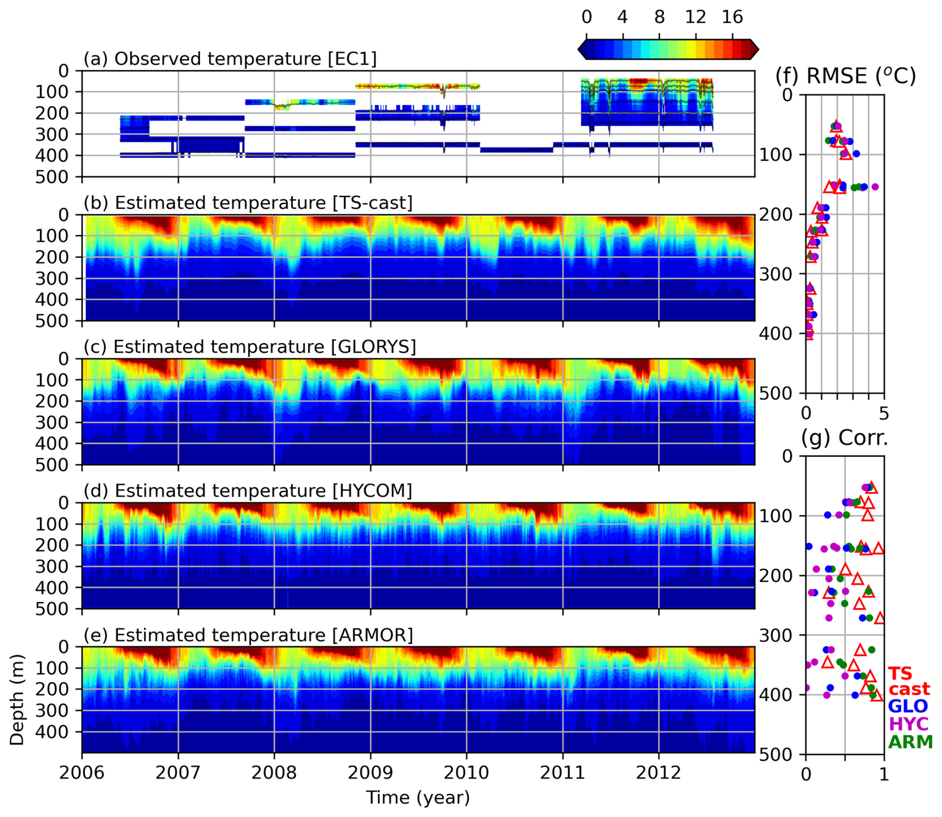
Figure 8 Time series comparison of observed and estimated temperature at the EC1 site. (a) Temperature observed at the EC1 mooring. Temperature as estimated by (b) TS-Cast, (c) GLORYS, (d) HYCOM, and (e) ARMOR3D. (f) Root Mean Square Error (RMSE) and (g) correlation coefficient (Corr.) with depth. In the side panels, red triangles indicate TS-Cast. Blue, magenta, and green dots represent the performance of GLORYS, HYCOM, and ARMOR3D, respectively.

To evaluate the model's ability to represent key vertically integrated properties of the water column and its variability, we validated its outputs against data from two arrays of PIES located in the EJS and the Kuroshio Extension (Fig. 9). These PIES arrays provide observations independent of ocean reanalysis data assimilation systems. PIES measures the round-trip acoustic travel time (τ), a proxy for the depth-integrated heat and salt content, thus providing a robust test of the model's baroclinic structure. In this study, the τ anomaly is used to isolate the baroclinic variability from the time-mean state. Since τ is dominated by water depth, using its anomaly facilitates a direct comparison of baroclinic signals across instruments deployed at different depths. We compared the observed τ anomaly against the τ anomaly calculated from the temperature and salinity profiles of TS-Cast, GLORYS, HYCOM, and ARMOR3D.

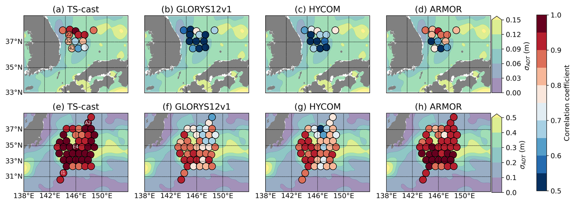
Figure 9 Temporal correlation coefficients between the vertical acoustic travel time (τ) from PIES observations and those calculated by the model results (TS-Cast, GLORYS, HYCOM, and ARMOR3D) for the (a–d) East/Japan Sea and (e–h) Kuroshio Extension arrays. Circle color indicates the correlation coefficient, while the background shading represents the standard deviation of ADT during the mooring periods. Correlation coefficients are shown only for sites where the WOA23 climatology is deeper than 700 dbar and the observation period is longer than one year.

The spatial distribution of temporal correlation coefficients (Fig. 9) reveals the performance of TS-Cast. Across both arrays, TS-Cast (Fig. 9a, e) demonstrates spatially coherent and remarkably high correlations with the PIES observations, with coefficients consistently exceeding 0.5 in the EJS and ranging from 0.8 to nearly 1.0 in the Kuroshio Extension. Similarly, ARMOR3D (Fig. 9d, h) also demonstrates high, spatially coherent correlations comparable to TS-Cast. In contrast, both GLORYS and HYCOM exhibit significantly lower and more spatially heterogeneous correlations. In many locations, particularly in the EJS, the correlation coefficients for GLORYS and HYCOM are close to 0.5 or even less, indicating a failure to capture the observed variability.

These statistics are further supported by direct time series comparisons at individual sites (Fig. 10). Visually, the τ anomaly from TS-Cast (red lines) closely tracks the observed variability (black lines), while the other reanalysis products show more incoherent high-frequency variability. For instance, at site P32 in the EJS, TS-Cast achieves a correlation of 0.81, whereas other reanalysis products score below 0.55. Similarly, at site A2 in the KESS array, TS-Cast's correlation of 0.95 is higher than that of GLORYS (0.75), HYCOM (0.78), and slightly higher than ARMOR3D (0.92). This comprehensive comparison confirms that TS-Cast more accurately captures the baroclinic variability integrated over the entire water column, a critical aspect of understanding ocean dynamics and heat content.

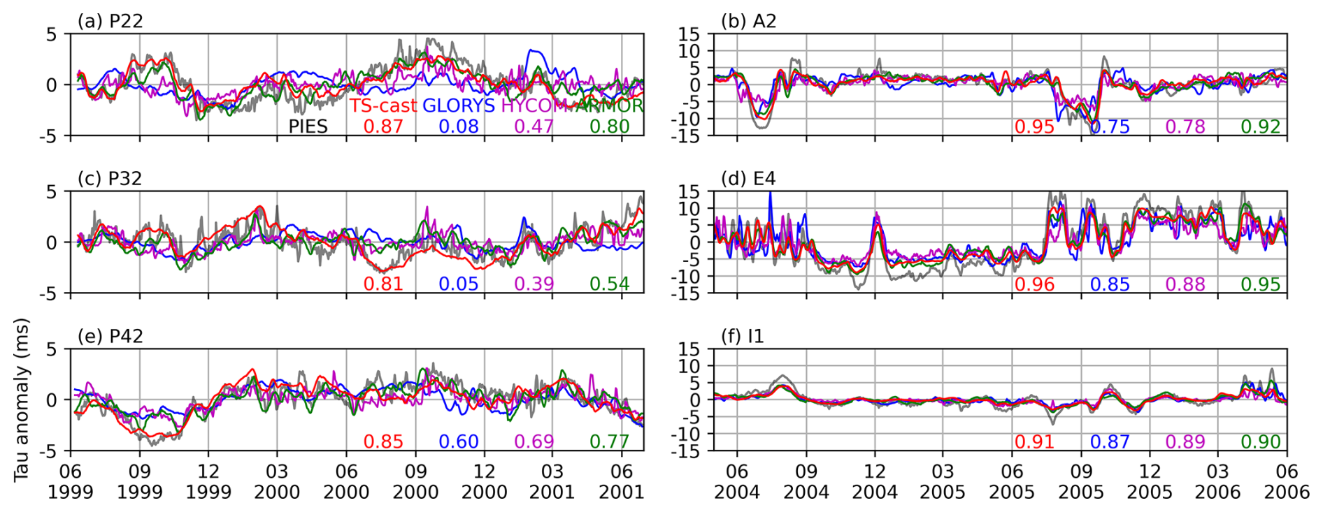
Figure 10 Time series of τ anomaly at selected PIES sites. Comparison between PIES observation (black), TS-Cast (red), GLORYS (blue), HYCOM (magenta), and ARMOR3D (green). Correlation coefficients for each model are shown in the bottom right of each panel. The locations of these sites are shown in Fig. 9.

4 Discussion

The comprehensive validation in this study demonstrates that TS-Cast, a purely data-driven model, consistently achieves performance comparable to, and often surpassing, that of established models such as the process-driven reanalysis, HYCOM and GLORYS, and the statistical reanalysis, ARMOR3D. Before interpreting these results, we address the distinction between spatial proximity and data leakage regarding the mooring-based validation. While the profiles exist near the KEO and EC1 mooring sites in the training set, these spatially and temporally scattered profiles do not constitute a leak of the mooring observations themselves. TS-Cast learns a general satellite-to-subsurface mapping function. The mooring validation tests a fundamentally different capability: reproducing continuous temporal variability over multiple years, which is information entirely absent from the training data. The PIES arrays provide the benchmark against which all models are evaluated under strictly equal conditions. PIES data are neither assimilated into any reanalysis product nor used in TS-Cast training. The fact that TS-Cast consistently outperforms all reanalysis products in this independent test confirms its genuine generalization capability. This section discusses the implications of these findings, interpreting the model's physical fidelity and inherent limitations as revealed by the validation analyses.

The model’s physical fidelity is most clearly elucidated by the coherence analysis (Figs. 11 and 12). At both the KEO and EC1 mooring sites, TS-Cast exhibits high coherence with observations for periods longer than approximately 16–32 d. This threshold robustly aligns with the characteristic timescales of mesoscale eddies, confirming that the model has successfully learned to translate the baroclinic signal in the input ADT data into a physically consistent subsurface thermohaline structure. The better performance of TS-Cast over the reanalysis models in this mesoscale band, particularly in the dynamically distinct EJS (Fig. 12), suggests that our data-driven approach offers a more efficient and perhaps less biased pathway for inferring subsurface structures from surface observations. This may be because TS-Cast avoids potential constraints inherent in process-driven models, such as imperfect initial conditions or sub-optimal data assimilation schemes.

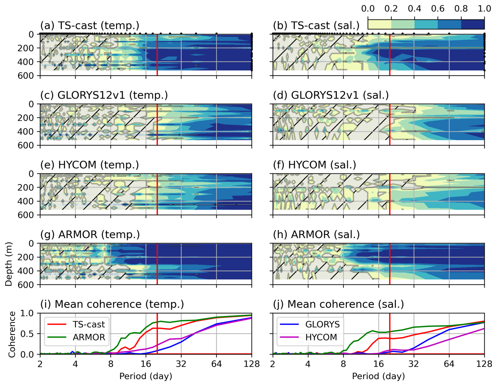
Figure 11 Coherence between observational data and model results at the KEO site. (a–h) Coherence distribution for temperature (temp.) and salinity (sal.) as a function of depth and period. Hatched areas indicate where the coherence is not above the 95 % significance threshold. (i–j) Averaged coherence over all depths. Red, blue, magenta, and green lines represent TS-Cast, GLORYS, HYCOM, and ARMOR3D, respectively. The vertical red line indicates a period of 20 d, and the horizontal red line indicates the 95 % significance threshold.

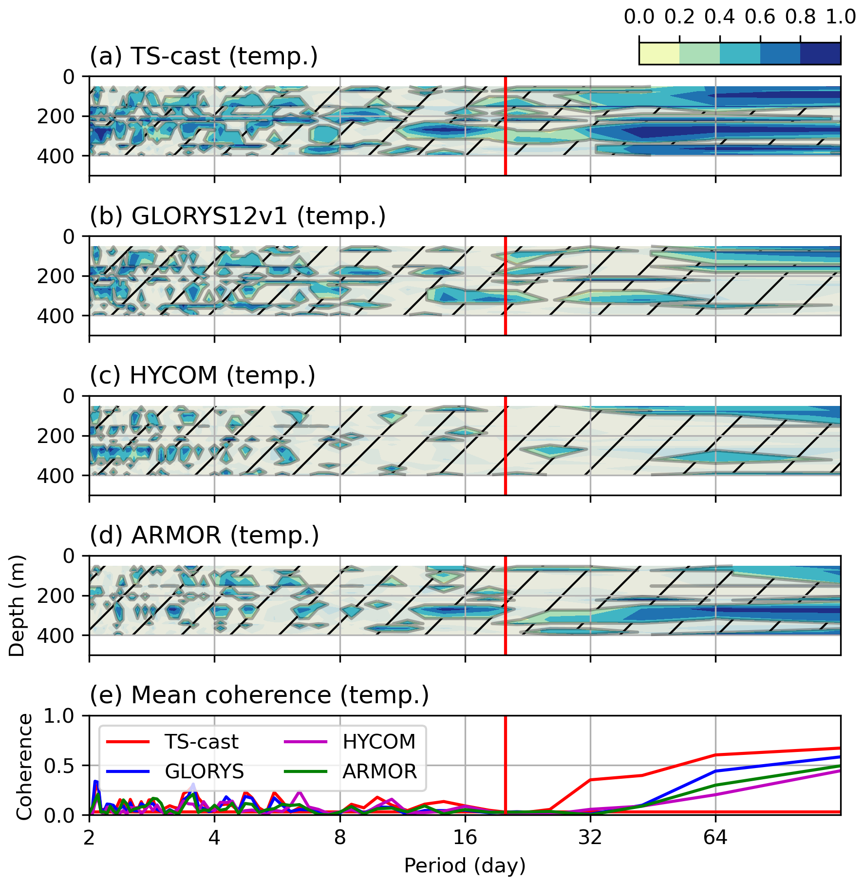
Figure 12 Coherence between observed temperature and model results at the EC1 site. (a–d) Coherence distribution for temperature as a function of depth and period. Hatched areas indicate where the coherence is not above the 95 % significance threshold. (e) Averaged coherence over all depths. Red, blue, magenta, and green lines represent TS-Cast, GLORYS, HYCOM, and ARMOR3D, respectively. The vertical red line indicates a period of 20 d, and the horizontal red line indicates the 95 % significance threshold.

Conversely, the sharp decline in coherence at periods shorter than ∼20 d is not an arbitrary model failure but an equally important finding that reveals the inherent limitations imposed by its input data. The model’s performance is fundamentally bounded by the information content of its inputs. The satellite ADT signal, while powerful, contains several sources of noise that are physically unrelated to the baroclinic TS structure the model aims to predict. These contaminating signals set a ceiling on the model's potential accuracy and explain the drop in high-frequency coherence. Two primary sources of this noise are:

1. Low temporal sampling rate of altimetry
   A fundamental limitation of satellite altimetry is its low temporal sampling rate, which prevents the resolution of high-frequency ocean variability. The Jason-series altimeters, for instance, have a repeat cycle of approximately 10 d. According to the Nyquist sampling theorem, this sampling interval can only unambiguously resolve signals with a period longer than 20 d. Consequently, important high-frequency processes, such as internal tides and inertial internal waves, are not captured in the satellite ADT record. The ADT data that serves as a primary input to the model fundamentally lacks reliable information on this high-frequency variability, making it physically impossible for the model to reconstruct these specific phenomena.

2. Barotropic and non-steric signals
   Satellite altimetry measures total SSH, which comprises both a baroclinic (steric) component, linked to subsurface TS structure, and a barotropic (mass-loading) component. The TS-Cast model is designed to reconstruct only the baroclinic variability; therefore, barotropic signals act as physically “unpredictable” noise. This non-steric variability is significant, accounting for approximately 10 % of the SSH variance in the KESS region (Park et al., 2012). It includes not only intrinsic bottom pressure fluctuations but also residual signals from high-frequency atmospheric forcing where the Dynamic Atmospheric Correction (DAC) is incomplete (Park et al., 2012). Collectively, these non-steric signals impose a fundamental limit on the model's accuracy, particularly at high frequencies.

Our comparisons with the ARMOR3D reanalysis highlight a critical methodological distinction. ARMOR3D is a data-assimilating product that incorporates the CORA dataset, which includes the OceanSITES mooring data, including KEO and EC1, used for our validation. This lack of data independence might explain ARMOR3D's near-perfect correlations (Figs. 6 and 7) and high coherence in the 8–16 d band at KEO (Fig. 11), especially upper 300 m depth where dense observations exist. The EC1 mooring comparison (Fig. 12) is therefore more revealing. At this site, TS-Cast, which does not directly assimilate subsurface observations at the prediction time, achieves a higher mean coherence than the ARMOR3D product. While we could not definitively verify whether EC1 data were included in the CORA dataset used by ARMOR3D and GLORYS, the fact that TS-Cast achieves coherence near 0.5 at periods longer than ∼30 d is significant. This result demonstrates TS-Cast's robust capability to reconstruct subsurface dynamics purely from satellite observations, performing comparably to or better than an assimilation-based model in this instance.

5 Conclusions

In this study, we developed and validated TS-Cast, a novel deep neural network model that estimates subsurface temperature-salinity (TS) profiles of the ocean using satellite remote sensing data. Despite being a purely data-driven model, TS-Cast demonstrated accuracy comparable to or exceeding that of state-of-the-art data-assimilating reanalysis models like HYCOM, GLORYS, and ARMOR3D. This was validated against long-term mooring observations in dynamically distinct regions, such as the Kuroshio Extension and the East/Japan Sea. In particular, its performance in reproducing the acoustic travel time (τ) variability from PIES, which represents the integrated property of the water column, confirms that the model accurately reconstructs the physical baroclinic structure of the water column.

Beyond developing a novel AI model, the core contribution of this work is the rigorous validation methodology we established to quantitatively define the model's physical fidelity and inherent limitations. Coherence analysis revealed that TS-Cast predicts mesoscale variability with periods longer than approximately 20–30 d with very high accuracy. This indicates that the model has successfully learned to translate the baroclinic information contained in the input absolute dynamic topography (ADT) data into a physically consistent internal ocean structure.

Conversely, the sharp decline in performance at higher frequencies (periods shorter than ∼20 d) is an equally important finding. This is not a flaw in the model itself but stems from the fundamental limitations of its input satellite altimetry data. Factors such as the low temporal sampling frequency of altimeters (the Nyquist limit), the barotropic signals unrelated to the TS profile, and incompletely corrected non-baroclinic components act as physical “noise” that is unpredictable for the AI model. Ultimately, the model's performance is fundamentally constrained by the quality and content of the information provided by its input data.

For studying mesoscale ocean phenomena, TS-Cast can be a powerful tool to supplement existing methods or even serve as an alternative. Furthermore, the rigorous validation framework presented here supplements existing spatial validation methods. By integrating both spatial (via Argo) and temporal (via moorings) validations, future studies can leverage a more comprehensive standard for evaluating the reliability of AI-based ocean prediction models.