Filamentogenesis and Filamentolysis of a Low-Density Filament: Dynamic Processes in the Near-Surface Ocean Under Tidal Forcing

This study investigates the dynamics and alteration of a low-density filament driven by freshwater-induced buoyancy embedded within a tidal mixing front, focusing on its spatial and temporal evolution in the near-surface layer (0.1–10 m) of the water column. A high-resolution, multi-sensor dataset, consisting of surface drifters, a drifting sensor chain, and an autonomous surface vehicle equipped with an Acoustic Doppler Current Profiler, temperature, and conductivity sensors, was used to observe patterns of divergence, vorticity, and vertical velocities. The measurements resolved three phases of the filament occurring on length scales of O(0.1–2 km) and time scales of minutes to one hour: (I) establishment of the filament in the overlying first meter and filamentolysis <1 m, (II) the ongoing filamentolysis in the lower NSL induced filamentogenesis above 0.6 m, (III) restratification of the upper 0.6 m. Vertical velocities ranged between $\pm \mathrm{20}\mathrm{m}{\mathrm{d}}^{-\mathrm{1}}$ with pronounced asymmetric responses on the filament boundaries due to the coupling of local filamentary kinematics and tide-induced vertical motions. In phase III, stratification allowed for increased heat uptake within the filament. These investigations highlight the role of the overlooked top surface layer in potentially altering the energy, heat, and gas budget of the ocean, which is critical for understanding the air–sea interface in the context of climate change.

1 Introduction

Low-density filaments, narrow, buoyant intrusions of warm or less dense water into denser surroundings, are a rarely observed but dynamically significant manifestation of frontal activity in the upper ocean. They form when frontal geometry, background flow, and strain orientation combine to elongate and pinch meanders into streamer-like features (Thomas et al., 2008). The strain field determines which side of the front is drawn out: when dense water extends into lighter water, a cold/dense filament forms, reinforced by downwelling from ageostrophic secondary circulation (ASC; McWilliams et al., 2009, 2015). In contrast, low-density filaments arise when buoyant water intrudes into denser regions, typically in regions of anticyclonic vorticity associated with the frontal jet, where horizontal convergence and shear help shape and elongate the filament (Mahadevan and Tandon, 2006; McWilliams et al., 2015; Garcia-Jove et al., 2022; Jakes et al., 2024). These features are short-lived: ASC upwelling spreads the buoyant anomaly above the mixed layer, while local stratification suppresses vertical replenishment, making lateral advection essential for their persistence (Jakes et al., 2024). Their horizontal scales are located between the mesoscale regime and small-scale three-dimensional turbulence (Chrysagi et al., 2021) with a vertical extent to the upper 50 m of the surface ocean (Thomas and Lee, 2005; Mahadevan and Tandon, 2006). Vertical velocities driving ASC may reach $\pm \mathrm{100}\mathrm{m}{\mathrm{d}}^{-\mathrm{1}}$, restratifying horizontal density gradients within subinertial time scales (Thomas and Lee, 2005; Chrysagi et al., 2021). Such asymmetries in formation and lifetime render low-density filaments both dynamically important and observationally elusive. Those findings apply well to dense/cold filaments that are investigated within various studies (e.g., McWilliams et al., 2009; Johnson et al., 2020; Chrysagi et al., 2021; Esposito et al., 2023). Some of them state the occurrence of low-density filaments and Lapeyre and Klein (2006) underscore the importance of filamental upwelling as develops at low-density filaments for the ocean nutrient flux. McWilliams et al. (2015) points to the rarity of low-density filaments, but otherwise frontal literature lacks a quantification from either models and in situ observations of this type of filaments.

The southern North Sea provides an ideal setting to study these processes. There, tides, wind forcing, and freshwater inputs create a highly energetic and deformable frontal environment. Tidal mixing fronts form at the interface between vertically stratified and well-mixed waters in summer, when surface heat flux steepens lateral temperature gradients (Van Heijst, 1986). Those fronts occur on continental shelves worldwide (Timko et al., 2019) and mediate exchanges of nutrients, particles, and energy between ocean layers (Thomas et al., 2008; Sun and Cho, 2010). In the North Sea, they vary seasonally under semidiurnal tides, fortnightly spring-neap cycles, bottom topography, and intermittent winds (Simpson et al., 1990; Holt and Umlauf, 2008; Zhao et al., 2019). Especially in the southern North Sea, freshwater input from rivers can lower coastal salinity by up to 10 g kg⁻¹ (Chegini et al., 2020), steepening density gradients and intensifying fronts (Simpson et al., 1990; Ricker et al., 2021; Goßmann et al., 2025). According to Núñez-Riboni and Akimova (2017) river-runoff is responsible for ∼80 % of the inter-annual salinity variability in the southern North Sea, both in terms of spatial extent and magnitude. Chegini et al. (2020) estimated the combined freshwater flux of the rivers Elbe, Weser, Ems and Eider to be 1200 m³ s⁻¹, however, Meyer et al. (2025) state that the river Elbe can afford a freshwater input up to $\sim \mathrm{1420}{\mathrm{m}}^{\mathrm{3}}{\mathrm{s}}^{-\mathrm{1}}$ alone in winter season. The additional freshwater mainly remains in the upper water column, forming a two-layer stratification (Stanev et al., 2014). This state persists depending on the freshwater flux added; Chegini et al. (2020) recorded a massive Elbe-runoff event ($>\mathrm{4000}{\mathrm{m}}^{\mathrm{3}}{\mathrm{s}}^{-\mathrm{1}}$) causing a continuous stratification in shallow waters (20–30 m; near the island of Helgoland) in summer 2013 that lasted 120 d. In combination with semidiurnal tides with tidal hubs exceeding ∼3.5 m (Meyer et al., 2025), an overturning estuarine circulation forms, where low-density surface water flows seawards and denser North Sea water propagates landwards near the bottom, oscillating with mixing during periods (Burchard and Badewien, 2015). Stanev et al. (2014) explain salinity to be responsible for 20 % of this overturning circulation, with the remaining drivers being winds, external salinity input (precipitation, inflow from adjacent seas and channels; Núñez-Riboni and Akimova, 2017). These cumulative processes and preconditions acting on horizontal density gradients, make fronts in the North Sea highly sensitive to mesoscale and submesoscale strain, a key prerequisite for frontogenesis (Garcia-Jove et al., 2022).

During frontogenesis, divergent flow (divergence) drives upward motion on the light side and convergent flow (convergence) downward motion on the dense side, flattening isopycnals and enhancing stratification, whereas reversed patterns lead to frontolysis. Analogous dynamics occur in narrow buoyancy filaments, where horizontal strain sharpens buoyancy gradients and drives ASC, a process referred to as filamentogenesis (McWilliams et al., 2009, 2015; Garcia-Jove et al., 2022; Jakes et al., 2024). This circulation acts to restore stratified balance but modifies the filament structure depending on its buoyancy anomaly: dense filaments are reinforced by surface convergence and central downwelling that deepen the anomaly to several hundred meters (e.g., Garcia-Jove et al., 2022), whereas low-density filaments experience reversed circulation that shoals buoyant water toward the surface (Thomas et al., 2008) and promotes rapid filament decay. In this study, “filamentogenesis of low-density filaments” is defined as the ASC-driven adjustment process acting on buoyant filaments, in which reversed circulation transports light water upward and outward, shoaling the buoyancy anomaly and leading to rapid filament weakening and decay as stratification is restored. Capturing these dynamics requires high-resolution measurements and calculation of Differential Kinematic Properties, such as divergence, vorticity, and horizontal velocity gradients, from water-column instabilities or path-integrated velocity gradient quantities (e.g., Vélez-Belchí and Tintoré, 2001; Molinari and Kirwan, 1975; Berta et al., 2016; Huntley et al., 2022). Surface drifters, radars, and ADCPs have been widely used (e.g., Hill et al., 1993; Shcherbina et al., 2013; Berta et al., 2016, Archer et al., 2020; Esposito et al., 2023), yet most studies lack data from the uppermost meter of the ocean, precisely where frontal and low-density filamentary processes peak (Thomas et al., 2008; Chrysagi et al., 2021; Gassen et al., 2023). Submesoscale features [O(0.1–10 km)] are critical for the ocean's energy cascade, both distributing energy forward and feeding larger scales (Schubert et al., 2020; Zhang et al., 2023). In shallow seas like the North Sea, these processes are assumed to be strongly imprinted at the surface, yet high-resolution observations remain scarce and temporally aliased (Johnson et al., 2020).

Building on this gap, we suggest that high freshwater contrasts in the southern North Sea generate the conditions necessary for low-density filament formation. Tidal oscillations may favour the export of dense filaments offshore into denser surroundings and alter filaments by alternately shearing, stretching, and compressing the density field. In these situations, transient anticyclonic strain zones can develop along the front, momentarily reversing the usual dense-offshore export and enabling warm-side water to intrude into the cold side. Although such low-density filament events are rarely observed, the unique tidal environment of the southern North Sea offers occasional opportunities to capture them. To test this hypothesis, we conducted high-resolution ADCP and CTD measurements at O(0.1–2 km) scales using an autonomous surface vehicle (ASV) at a tidal mixing front in the southern North Sea. Trajectories from 14 surface drifters and a drifting sensor chain complemented these observations, resolving the evolution of a low-density filament with a focus on the near-surface layer (NSL; 0.1–10 m). This dataset allows us to investigate the buoyancy-driven nature of the filament and the role of tidal modulation in amplifying and weakening its surface divergence signal, providing new insight into these dynamically important features.

2 Materials and Methods

2.1 Data acquisition

During cruise HE626 on RV Heincke, a multi-platform dataset combining ship-based, autonomous, and Lagrangian observations was collected. Central to the study were measurements by the ASV Halobates (Wurl et al., 2024), which provided current velocities in the NSL as well as high-resolution temperature and salinity profiles. Additional underway observations included wind data and continuous NSL hydrographic measurements (temperature and conductivity) from a 4H Jena Engineering Pocketbox Ferrybox flow-through system. Stationary measurements consisted of ship-based Seabird SBE911+ CTD casts and deployments of Lagrangian platforms, including 14 near-surface drifters (Meyerjürgens et al., 2019) and a drifting sensor chain. The focus of this study is on observations from 5 August 2023, northwest of Helgoland (Fig. 1a), targeting submesoscale frontal processes under freshwater input from the Weser and Elbe estuary and strong semidiurnal tidal influence. The region was characterized by tidal mixing front structures on scales of O(0.1–10 km), visible in sea surface salinity (SSS). The more saline water mass originated from the open North Sea, while the fresher mass consisted of a mixture of North Sea water and river runoff from the German Bight (Burchard and Badewien, 2015). Semidiurnal tides imported saline offshore water, creating horizontal gradients of up to $\pm \mathrm{1.5}\mathrm{g}{\mathrm{kg}}^{-\mathrm{1}}$ (Fig. 1a). The frontal system exhibited submesoscale meanders (Fig. 1a) and developed a low-density filament on horizontal scales of 0.1–2 km (Fig. 1c).

Front detection was performed by observing satellite-based sea surface foundation temperature (CMEMS, 2023) and guided by SSS fields from the CMEMS Atlantic-European Northwest Shelf Ocean Physics Analysis and Forecast model (CMEMS, 2024), which has a horizontal resolution of $\sim \mathrm{3}\mathrm{km}\times \mathrm{3}\mathrm{km}$ and hourly output. For the target region, model SSS correlated reasonably with in situ Ferrybox salinity (R=0.71; Fig. B1). On the evening of 4 August, the vessel carried out a zig-zag survey (∼7 kn) to validate the model fields and identify the strongest gradient, which reached $\mathrm{\Delta }\text{SSS}\approx \mathrm{1.2}\mathrm{g}{\mathrm{kg}}^{-\mathrm{1}}{\mathrm{km}}^{-\mathrm{1}}$. In situ salinity was obtained from the Ferrybox, pumping seawater from 3 m depth ($\sim \mathrm{6}\mathrm{L}{\min }^{-\mathrm{1}}$) with conductivity measurements accurate to $\pm \mathrm{0.3}\mathrm{mS}{\mathrm{cm}}^{-\mathrm{1}}$. Once the gradient was confirmed, the vessel remained on station to deploy the Lagrangian instruments. A sensor chain equipped with six Sea&Sun CTM 48M CTDs mounted between 0.2–10 m depth, transmitting position data every 2 min (Garmin inReach Messenger GPS), and 14 surface drifters transmitting positions every 5 min (SPOT Trace^® GPS). The drifters were deployed by zodiac in the form of 12 triangular arrays (Fig. 1b) and tracked over 25 h. Their trajectories showed a north-westward drift under prevailing southeasterly winds (Fig. C12), covering ∼21 km, while their rotary motion reflected tidal currents (Meyerjürgens et al., 2020). During ebb tide, drifters were displaced westward at speeds up to 1 m s⁻¹ , an effect intensified by wind forcing between 14:00–21:00 UTC when wind speeds increased from 6–14 m s⁻¹. The sensor chain largely followed the drifter displacement.

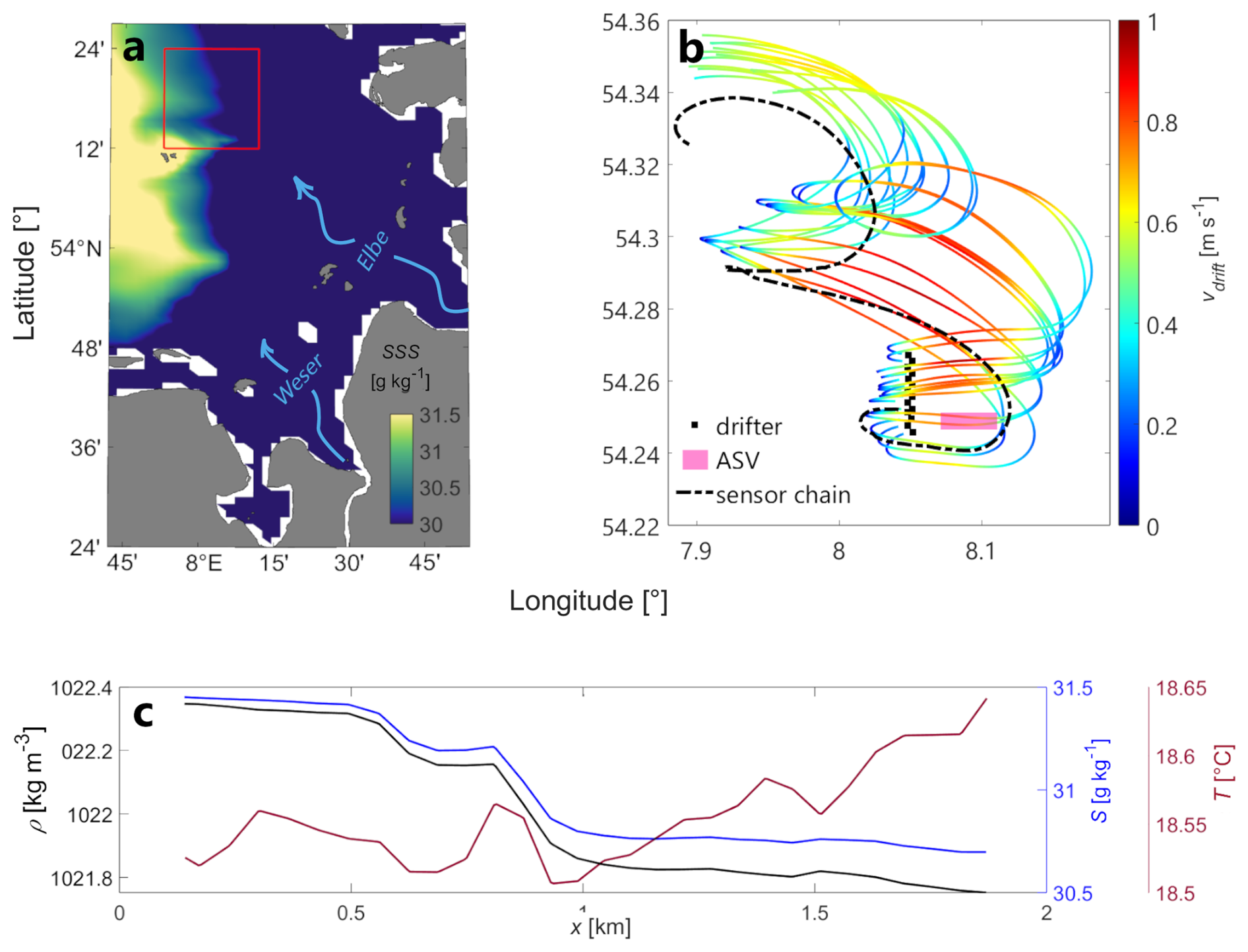
Figure 1 (a) The study site is located in the southern North Sea, northeast of Helgoland, highlighted with a red box. On 5 August 2023, the area exhibits submesoscale structures (low-density filament) with SSS gradients of $\pm \mathrm{1.5}\mathrm{g}{\mathrm{kg}}^{-\mathrm{1}}{\mathrm{km}}^{-\mathrm{1}}$. (b) Measurements within the red box include a drifting sensor chain (black dot-dashed line), 14 Lagrangian surface drifter deployments (initial positions as black squares) and the ASV (pink area). Drifter trajectories are colored by current velocity magnitude. (c) Density (black line), salinity (blue line) and temperature (red line) of the filament sampled by the ASV.

After the Lagrangian deployments, the ASV was launched within the frontal zone to observe the propagation of the low-density filament at high temporal resolution. The vehicle executed a repeating rectangular track (∼2 km east–west, 0.08 km north–south), with only the east–west transects analyzed (Fig. 1c). Seven transects were completed between 06:30 and 12:45 UTC at ∼2 kn. The ASV carried a Teledyne RD Instruments RiverRay 600 kHz ADCP, mounted at 0.275 m immersion depth. With a 1 m vertical bin size, velocity profiles were obtained from 1–10 m depth (excluding near-bottom bins). Thus, ADCP data began at 1 m and extended through the NSL, but did not cover the overlying surface layer. In contrast, the ASV was equipped with seven Idronaut OS310 CTDs mounted at 80–100 µm (denoted the skin layer; Shinki et al., 2012), 30, 40, 50, 60, 85, and 100 cm. Those resolved temperature and salinity changes within the skin layer down to one meter of the water column, allowing the evolution of the filament surface expression to be captured in detail. The ASV is equipped with rotating glass plates that pick up the skin layer by surface tension followed by scrapes transferring the water into the tube system being connected to the CTDs. Because of this setup, the CTDs and ADCP provided complementary rather than overlapping coverage: CTDs focused on the upper meter, while the ADCP recorded current velocities in the deeper part of the NSL.

For analysis, ADCP data were filtered to remove outliers (>3σ from the mean), truncated below 10 m depth, and smoothed using a 60 s moving average. Drifter positions were post-processed following Deyle et al. (2024), yielding interpolated trajectories with a uniform 5 min resolution, including bridging of GPS gaps up to 1 h.

2.2 Surface divergence from drifters

A variety of studies have estimated divergence by tracking the deformation of drifter clusters (Molinari and Kirwan, 1975; Kawai, 1985; Berta et al., 2016; Tarry et al., 2021; Huntley et al., 2022; Esposito et al., 2023). Molinari and Kirwan (1975) introduced two robust approaches: (a) the method of least squares, which infers divergence from velocity gradients fitted around the cluster centroid, and (b) the area-based method, which calculates divergence from the rate of change in the polygonal area spanned by a drifter group. While the least-squares method scales well to larger clusters and offers higher statistical confidence (Molinari and Kirwan, 1975; Tarry et al., 2022), it requires more drifters and is sensitive to tidal modulation of trajectories, which can obscure frontal signatures. The area-based method is less demanding, relying on only three drifters, and is therefore better suited for frontal environments where deformation rates are high. In this study, we applied the latter, expressed as

$$\begin{array}{}\text{(1)}& \mathit{\delta }={\displaystyle \frac{\mathrm{1}}{A}}{\displaystyle \frac{\partial A}{\partial t}}\end{array}$$

where A is the area of a drifter triplet and $\partial A/\partial t$ its temporal change.

To maximize the number of usable triplets, drifters were deployed on 5 August 2023 as vertices of 12 potential triangles with edge lengths of 0.2–0.5 km along a ∼4 km transect (Fig. 1b). Only complete triplets were retained, excluding 21.8 % of deployments with <3 drifters. Because high-gradient fronts coincide with elevated strain rates (Mahadevan and Tandon, 2006), clusters in such areas were particularly prone to rapid elongation and biased divergence estimates. To address this, Berta et al. (2015, 2016) and Huntley et al. (2022) proposed quality metrics that characterize triangle geometry. One such measure is

$$\begin{array}{}\text{(2)}& \mathrm{\Lambda }={\displaystyle \frac{\mathrm{12}\sqrt{\mathrm{3}}A}{P^{\mathrm{2}}}}\end{array}$$

where P is the perimeter. Λ=1 corresponds to equilateral triangles, while Λ=0.2 indicates near-collinear configurations. Huntley et al. (2022) demonstrated that Λ provides slightly more reliable results than internal-angle metrics (θ, γ), with ∼4 % better accuracy. Given the limited sample size (∼20 triplets per time step), this improvement was significant. Applying a conservative filter of $\mathrm{0.2}\le \mathrm{\Lambda }\le \mathrm{1}$ retained 36.4 % of the available clusters, leaving 3559 valid triplets for divergence estimation. Overlaps in drifter trajectories in highly dynamic regimes (e.g., tidal transitions or wind-driven surges; Fig. 2b) further reduced the number of suitable triplets (Berta et al., 2016; Villa Castrillón et al., 2024).

Divergence was then calculated for each triplet centroid using Eq. (1). Triplets were time-binned according to tidal phase, since tidal reversals prevented uniform resampling (calculation of divergence from clusters every 15 min; Esposito et al., 2023). Five intervals were identified (t₁–t₅: 1.5, 5, 7.5, 5.5, 5.5 h), this study however, focuses on t2 as this was the period for detecting the low-density filament. Delaunay triangulation at the start of each interval increased usable triplets and avoided configurations already deformed. Divergence estimates were subsequently gridded onto a 1 km×1 km grid, averaging values within each spatial bin and time interval. This yielded 2179 triplets suitable for analysis. Finally, divergence values were normalized by the Coriolis frequency $f=\mathrm{1.18}\times {\mathrm{10}}^{-\mathrm{4}}{\mathrm{s}}^{-\mathrm{1}}$ at a reference latitude of 54.25° N.

2.3 Water column properties and instabilities from drifting sensor chain and ASV CTDs

Since the sensor chain trajectory broadly followed the drifters, it provided an additional basis to investigate water column structure and instabilities at the front. To characterize the water masses shaping the front, temperature and conductivity from the chain sensors were converted to conservative temperature, absolute salinity, and in-situ density at depths $z=[\mathrm{0.2},\mathrm{1.2},\mathrm{6.2},\mathrm{8.4},\mathrm{10.6}]\mathrm{m}$. The same procedure was applied to the ASV CTD data at depths $z=[\mathrm{0.0001},\mathrm{30},\mathrm{40},\mathrm{50},\mathrm{60},\mathrm{85},\mathrm{100}]\mathrm{cm}$. These profiles were then used to derive water column instability proxies: the Brunt–Väisälä frequency

$$\begin{array}{}\text{(3)}& N^{\mathrm{2}}={\displaystyle \frac{\partial b}{\partial z}},\end{array}$$

and the lateral buoyancy gradient

$$\begin{array}{}\text{(4)}& M^{\mathrm{2}}={\displaystyle \frac{\partial b}{\partial x}},\end{array}$$

with buoyancy defined as $b=g(\mathrm{1}-\mathit{\rho }/{\mathit{\rho }}_{\mathrm{0}})$, where ρ is potential density and ${\mathit{\rho }}_{\mathrm{0}}=\mathrm{1022.3}\mathrm{kg}{\mathrm{m}}^{-\mathrm{3}}$ is the surface reference density. By examining the evolution of isopycnal slopes, periods of restratification and mixing could be identified.

2.4 Divergence from ASV-mounted ADCP

To investigate frontal dynamics at the lower end of the submesoscale and at high temporal resolution, divergence was also calculated from the ADCP mounted on the ASV. Following Rudnick (2001), the assumption of a frontal jet aligned with the front allows for the simplification of the full divergence term $\mathit{\delta }=\frac{\partial u^{\ast }}{\partial x}+\frac{\partial v^{\ast }}{\partial y}$ (where u^∗ and v^∗ are the cross- and along-front velocity components) to:

$$\begin{array}{}\text{(5)}& \mathit{\delta }\approx {\displaystyle \frac{\partial u}{\partial x}},\end{array}$$

a formulation commonly known as the “one-ship method” (Shcherbina et al., 2013). This approach has been widely applied to ADCP data for single-depth divergence estimates (e.g., Drinkwater and Loder, 2001; Archer et al., 2020; Esposito et al., 2023).

From the ASV-mounted ADCP, the along-track velocity component was extracted (along-track velocities resemble across-front velocities) and organized into transects (Fig. 1c). Data were averaged onto a grid with 10 m horizontal spacing, 2 min temporal resolution, and 1 m vertical intervals before applying Eq. (5), and the resulting divergence estimates were normalized by the Coriolis frequency f. To capture the temporal evolution of the low-density filament, full-depth transects were analyzed at three times during the morning sequence ([$t\mathrm{1}=\mathrm{07}:\mathrm{23}$, $t\mathrm{2}=\mathrm{07}:\mathrm{40},$ $t\mathrm{3}=\mathrm{08}:\mathrm{30}$] UTC). In addition to horizontal divergence, the vertical component of relative vorticity,

$$\begin{array}{}\text{(6)}& \mathit{\zeta }={\displaystyle \frac{\partial v}{\partial x}}-{\displaystyle \frac{\partial u}{\partial y}},\end{array}$$

was derived using the same method, together with the along-front velocity v. Surface density transects from the ASV CTD at z=1 m were analyzed for the same times, alongside co-located depth sections of δ, ζ, and v. Vertical velocity fields were overlaid to highlight frontogenesis and frontolysis processes (see Sect. 2.5).

2.5 Vertical velocity from drifter and ADCP divergence estimates

Vertical velocities in the water column were derived from the continuity equation including the term for divergence, which was previously calculated for drifters and ADCP:

$${\displaystyle \frac{\partial u}{\partial x}}+{\displaystyle \frac{\partial v}{\partial y}}+{\displaystyle \frac{\partial w}{\partial z}}=\mathrm{0},$$

which can be rearranged to

$$\begin{array}{}\text{(7)}& \mathrm{\Delta }w=-{\int }_{-z}^{z_{\mathrm{0}}}\left({\displaystyle \frac{\partial u}{\partial x}}+{\displaystyle \frac{\partial v}{\partial y}}\right)\mathrm{d}z,\end{array}$$

where Δw is the vertical velocity difference between the surface (z₀) and depth z. For drifters, the target depth was set to $z=-\mathrm{0.5}\mathrm{m}$, corresponding to the drifter's immersion depth (Meyerjürgens et al., 2019). At the surface, previous studies (Tarry et al., 2021; Rypina et al., 2021; Tarry et al., 2022; Esposito et al., 2023) assumed $w(z_{\mathrm{0}}=\mathrm{0})=\mathrm{0}\mathrm{m}{\mathrm{d}}^{-\mathrm{1}}$, as vertical motion at the surface is typically one to two orders of magnitude smaller than observed subsurface velocities. Rypina et al. (2021) argued that sea surface displacement is largely governed by gravity and tidal waves, yielding negligible vertical motion in the Mediterranean. In contrast, the North Sea exhibits much larger tidal amplitudes. Around Helgoland, the M2 tide causes vertical displacements of ∼1.5 m (Stanev et al., 2014), making the tidal-induced vertical velocity at the surface comparable to observed w. Thus, the assumption $w(z_{\mathrm{0}}=\mathrm{0})=\mathrm{0}\mathrm{m}{\mathrm{d}}^{-\mathrm{1}}$ was not valid here. Instead, sea surface height (SSH) with a rout-mean-square difference of ∼5–15 cm from CMEMS model data (CMEMS, 2024) was used to estimate tidal vertical velocities at z₀, applied as hourly means. For ADCP data, vertical velocities were calculated across the full depth range using Eq. (7). In this case, the one-ship method (Eq. 5) was substituted for the full divergence term, yielding:

$$\begin{array}{}\text{(8)}& w\left(z_i\right)=w\left(z_{i-\mathrm{1}}\right)+\left({\displaystyle \frac{\mathrm{d}u}{\mathrm{d}x}}\right)\mathrm{\Delta }z,\end{array}$$

where $\mathrm{d}u/\mathrm{d}x$ is the along-track divergence and Δz the ADCP bin size. A detailed derivation of Eq. (8) is provided in Appendix A. Since ADCP measurements begin at 1 m depth, tidal integration at the surface was unnecessary; the first estimate of w could be calculated directly at 2 m.

3 Results

3.1 Water column characteristics and instabilities from drifting sensor chain

During the high tide period between 09:00 and 12:00, the sensor chain crossed the low-density filament, which was observed from the surface down to ∼4–5 m and exhibited a density difference about 0.4 g kg⁻¹. It was embedded at the lower boundary of the tidal mixing front salinity signal ($\sim \mathrm{31.5}\mathrm{g}{\mathrm{kg}}^{-\mathrm{1}}$) and at the highest boundary of the temperature signal (∼19.0 °C), confirming its formation on the light side of the front. The filament persisted for approximately 3 h, showing a two-layer stratification from 09:00–12:00, with fresh (warm) water overlying more saline (cold) water. During the first two hours, the upper, lighter layer extended down to ∼4 m and retreated to ∼2 m in the final hour. This retreat was driven by a decrease in the salinity gradient while the temperature gradient increased (Fig. 2b and c). Around 17:00, the sensor chain crossed to the dense side of the front, where the filament was no longer apparent in salinity, temperature, or density.

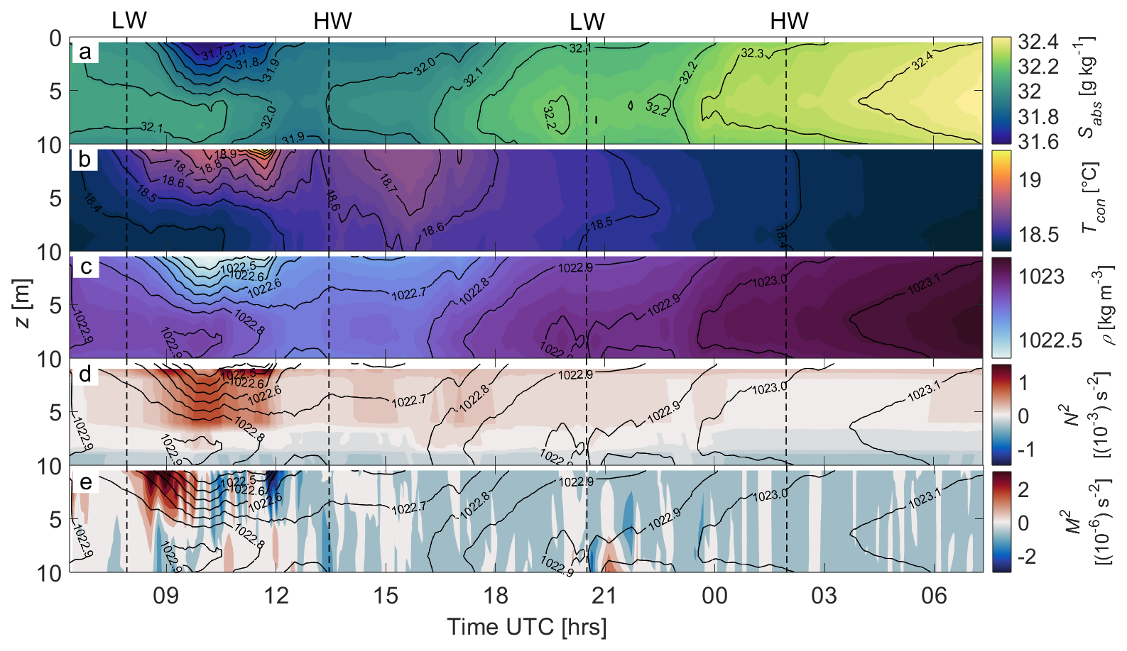
Figure 2 Time series of (a) absolute salinity, (b) conservative temperature, (c) potential density, (d) Brunt–Väissälä frequency N² and (e) lateral buoyancy gradient M² obtained from the drifting sensor chain during 5 and 6 August. Vertical black dashed lines mark low water (LW) and high water (HW). N² and M² are displayed with overlain isopycnals. The low-density filament can be observed between the first LW and HW.

The filament also influenced water column stability, evident in the Brunt–Väisälä frequency (N²) and lateral buoyancy gradient (M²). The low-density filament emerged from the surrounding tidal mixing front as a region of strongly positive N² (Fig. 2d), indicating stable stratification. Below 7 m, negative N² values suggested local buoyancy production, likely caused by vertical shear acting on horizontal density gradients near the bottom, possibly due to tidal interactions with topography. This feature correlated with the bifurcation of isopycnals (“forking”), where dense water was forced over lighter water, a property appearing along the entire time series rather than being unique to the filament. Considering the lateral buoyancy gradient (Fig. 2e), M² was positive (stable) when the filament was at ∼4 m depth, but reversed to negative values during its retreat, indicating buoyancy production and the upward displacement of the filament. This asymmetry will be further discussed in Sect. 3.4.

3.2 Coupling of filamentary and tide-induced vertical motions

Drifter triplet centroid trajectories from t2 over SSS isohalines (CMEMS, 2024, panel a) are shown in Fig. 3, along with space- and time-binned near-surface horizontal divergence normalized by f (Fig. 3b) and vertical velocity w (Fig. 3c). As the drifters crossed isohalines, these data reveal across-front divergence and corresponding areas of up- and downwelling. Both SSS and drifter trajectories indicate that the tidal mixing front meandered on the mesoscale along the tidal wave direction, while a sudden southward diffraction of the northern trajectories around 8.05° E longitude suggests a submesoscale low-density filament.

Following the main high tide current eastward (Fig. 3a), most drifters initially diverged with δ≈2f due to accelerating tidal flow (Figs. 3b and 1b). Shortly before 10:00, the northern cluster entered a convergence zone ($\sim -\mathrm{2}f$), then peaked at 5f after ∼30 min, and dropped to −5f around 11:00. Although δ ≈ ±5f is high relative to previous studies (Berta et al., 2016; Tarry et al., 2021, 2022), strong triplet deformation due to the tides likely caused overestimation (see Sect. 2.2). Divergence drove low-density filament water upward away from the axis, while dense water sank during convergence (Fig. 3c), with vertical velocities ranging from $\sim -\mathrm{30}$ – 50 m d⁻¹. Despite potential overestimation due to error propagation from the divergence estimation $(\stackrel{\mathrm{‾}}{\mathrm{\Delta }\mathit{\delta }/f}\approx \mathrm{2.928})$, the vertical velocity pattern aligns with the drifter centroid trajectories, including the southward diffraction at 8.05° E longitude. This behavior indicates the northern cluster sampled the low-density filament in the same time frame and tidal phase consistent with sensor chain observations (Fig. 2). The steepening of isopycnals (Fig. 2c) matches downwelling, while the sensor chain's decreasing vertical filament extent coincides with drifter-indicated upwelling.

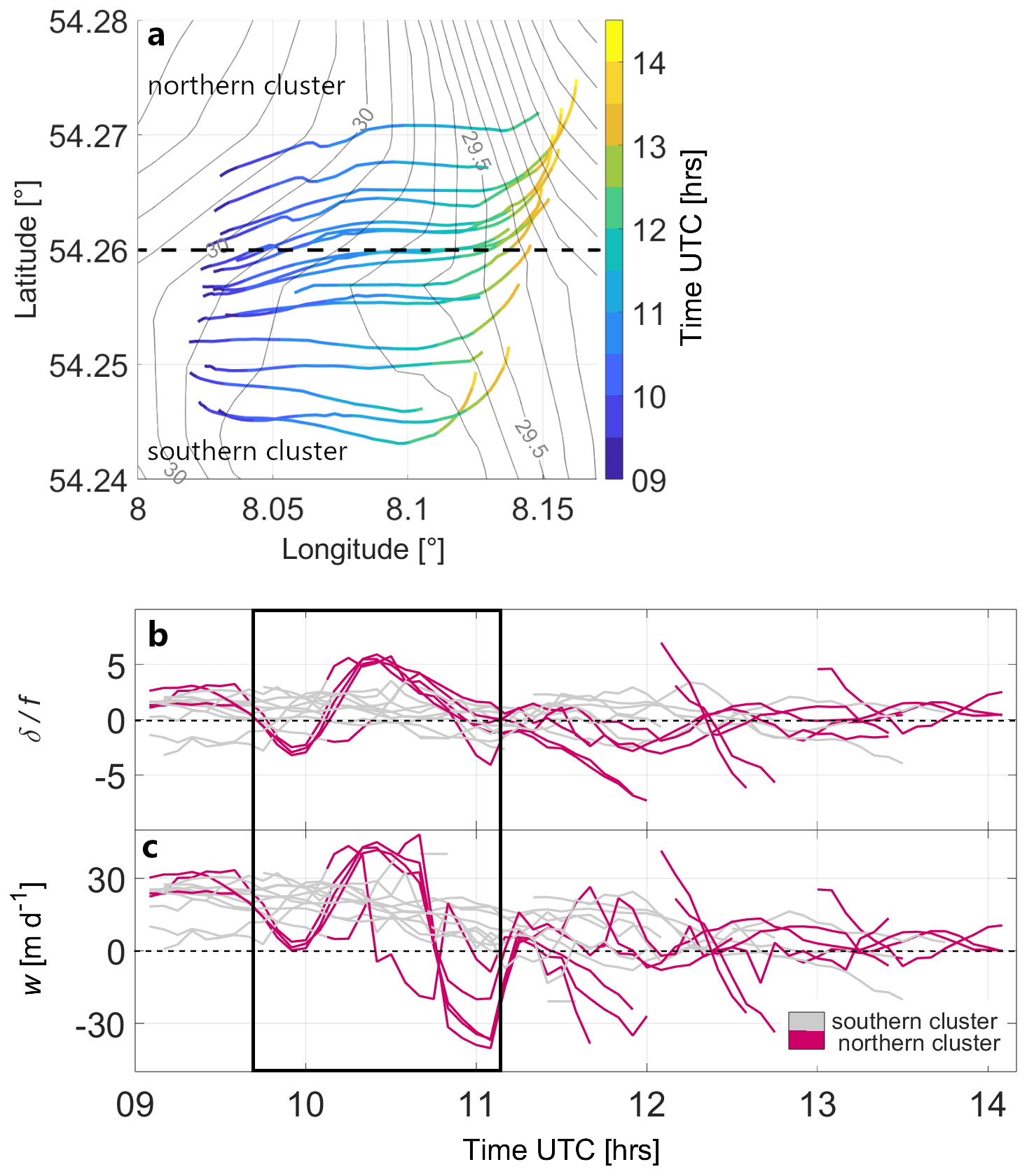
Figure 3 Divergence and vertical velocity patterns observed during high tide period. (a) Trajectories of the centroids from drifter triplets over latitude and longitude colored according to time on 5 August. The map background displays the corresponding isohales in g kg⁻¹ (CMEMS, 2024; gray solid lines) as mean over the displayed drifter period. (b) Normalized near-surface divergence and (c) vertical velocity in m d⁻¹ for the time sections of drifter triplets in (a) colored according to northern (magenta) and southern (grey) drifter triplet clusters. Black outlines highlight the observation of the filament.

The southern cluster showed weaker divergence, generally fluctuating between ±2f. At the filament location, these centroids did not display the diffraction seen in the northern cluster and remained on the 29.8 g kg⁻¹ isohaline during peak tidal flow, whereas the northern cluster crossed diapycnally by $\sim -\mathrm{0.5}\mathrm{g}{\mathrm{kg}}^{-\mathrm{1}}$. Outside the filament, w exhibited an overall up- to downwelling trend for both clusters, reflecting decreasing tidal velocities (Fig. 3b). In regions of filament-induced vertical motion, tides either mediated or amplified w (Fig. 4). For example, during the first convergence zone, filamentary downwelling was partly offset by tide-induced upwelling, while in the second convergence period, weaker tidal flow enhanced downwelling. Sharp discontinuities observed outside the filament (∼12 h) likely resulted from a secondary crossing of strong density gradients.

The contribution of tidal modulation to divergence is shown in a simplified model (spatially averaged means of divergence from drifter clusters) of the overall observed divergence, local filament divergence and tidal divergence (Fig. 4). After removing the local filament divergence δ(w_drift,SSH=0), where no tidal displacement was incorporated, from the overall divergence δ(w_drift), the remaining tide-induced divergence $\mathit{\delta }\left(w_{\text{tide},{\text{SSH}}_i}\right)$ indicates a reverse relation to the tidal phase of the high water. At early flood period ($\sim \mathrm{11}:\mathrm{30}$) divergence is added to the system, whereas at late flood period, when the tidal current decelerates, convergence is added. For the local filament divergence dynamics this may cause an offset up to ± 3f. Nevertheless, the functionality of this model is limited to the water surface and the resolution of the SSH data and needs further improvement to increase the quality of estimating the tide-induced divergence contribution.

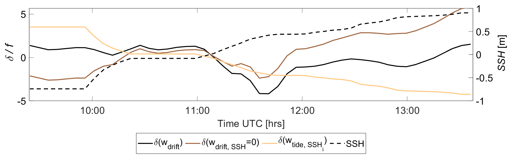
Figure 4 Time series of spatially-averaged divergence normalized by fcalculated from drifter triplets incorporating tidal displacement (black bold line) and excluding tidal displacement (w₀(z=0); brown line). Subtracting both divergence modes results in divergence budged resulting only from tidal displacement (yellow line). All modes are displayed in relation to the tidal phase indicated by SSH (black dotted line).

3.3 Filament structure and evolution of isopycnals in the overlying first meter

While with the data analyzed in Sects. 3.1 and 3.2 identified the low-density filament during the high tide period, data by the ASV (Sects. 3.3 and 3.4) address the filament observed during low tide. During this period, three phases were recognized in the evolution of the low-density filament in the overlying first meter of the NSL (Fig. 5). Panels a, d, g show phase I, where isopycnals were vertically aligned and density varied by about 0.4 kg m⁻³ over less than 0.5 km. Although data are only available for x<1.5 km, profiles at t1 reveal a fresh (30.6 g kg⁻¹ ) and cold (18.6 °C) filament core at $\mathrm{1.0}\mathrm{km}<x<\mathrm{1.5}\mathrm{km}$, contrasting with surrounding water masses along the transect. Density gradients were due to 10 times stronger influence of salinity ($\mathrm{\Delta }\mathit{\rho }\left(S\right)\approx \mathrm{0.54}\mathrm{kg}{\mathrm{m}}^{-\mathrm{3}}$) than temperature ($\mathrm{\Delta }\mathit{\rho }\left(T\right)\approx \mathrm{0.04}\mathrm{kg}{\mathrm{m}}^{-\mathrm{3}}$) (not shown), identifying the low-density filament as salinity-driven due to high freshwater contrasts.

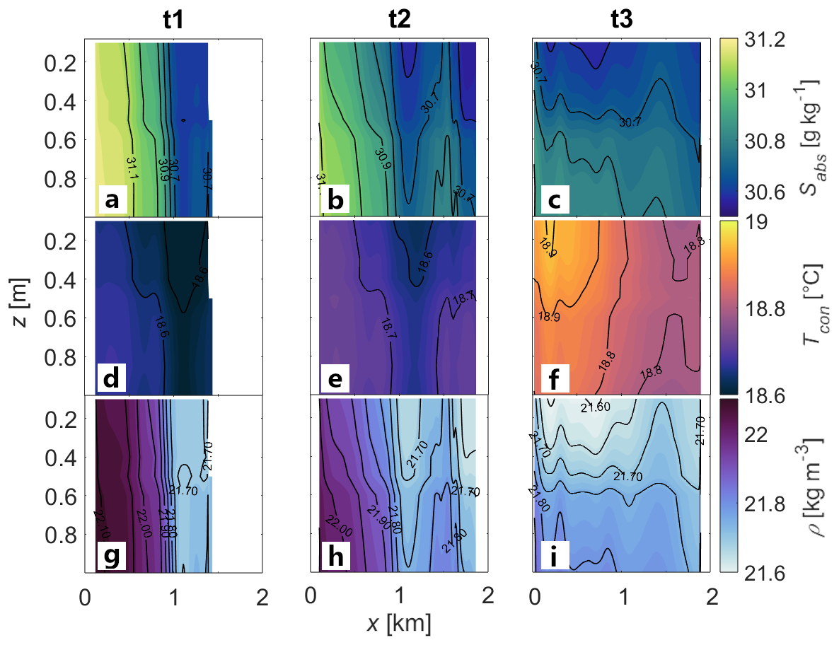
Figure 5 CTD data from the ASV displayed as contour section over depth across the filament at [$t\mathrm{1}=\mathrm{07}:\mathrm{23}$ am, $t\mathrm{2}=\mathrm{07}:\mathrm{40}$ am and $t\mathrm{3}=\mathrm{08}:\mathrm{30}$] UTC, each for of (a–c) absolute salinity, (d–f) conservative temperature and (g–i) potential density in the upper NSL.

In phase II (t2; Fig. 5b, e, and h), isopycnals above 0.6 m began to flatten away from the filament axis, and the light core of the filament shifted into the upper layer above 0.6 m, with a slight intensification of about 0.1 kg m⁻³ (Fig. 5h). Below 0.6 m, no flattening occurred, but the temperature gradient decreased, with a minor reduction in salinity (Fig. 5b and e). This led to compression of the filament core, reducing its horizontal extent in this layer to roughly half of its initial length. Phase III (t3; Fig. 5c, f, and i) occurred less than one hour later. Isopycnals were now nearly horizontal, and the low-density filament core was distributed homogeneously in the upper 0.6 m (Fig. 5i). Salinity followed the density pattern, while temperature became horizontally stratified with a gradient of ∼0.2 °C.

Throughout the observation period, the filament core salinity remained at 30.6 g kg⁻¹ (Fig. 5a–c), while the surrounding water mass decreased by $\sim \mathrm{0.4}\mathrm{g}{\mathrm{kg}}^{-\mathrm{1}}$. Temperature within the filament increased by ∼0.3 °C, compared to ∼0.1 °C in the surrounding water (Fig. 5d–f). Salinity primarily controlled density, which decreased by $\sim \mathrm{0.1}\mathrm{kg}{\mathrm{m}}^{-\mathrm{3}}$ within the filament and $\sim \mathrm{0.3}\mathrm{kg}{\mathrm{m}}^{-\mathrm{3}}$ in the surrounding water (Fig. 5g–i). The observed evolution of the low-density filament exhibits characteristics reminiscent of filamentogenesis, including upward displacement of the light core and lateral compression. Unlike classical cases of dense/cold filaments documented in the literature (e.g., McWilliams et al., 2015; Chrysagi et al., 2021; Jakes et al., 2024), these dynamics are driven primarily by salinity gradients rather than temperature gradients, reflecting the strong influence of freshwater input and tidal modulation in the southern North Sea. While ASC patterns are not yet analyzed, these observations suggest the filament is undergoing a process analogous to filamentogenesis, to be further confirmed with ADCP-derived velocity fields in the following section. Notably, the upward displacement of the filament core is consistently observed across all datasets: the sensor chain covering the NSL below 1 m, the drifter trajectories, and the ASV CTD measurements in the upper meter, reinforcing the robustness of this evolution.

3.4 ASC patterns and evolution of divergence, vorticity and vertical velocity in the NSL

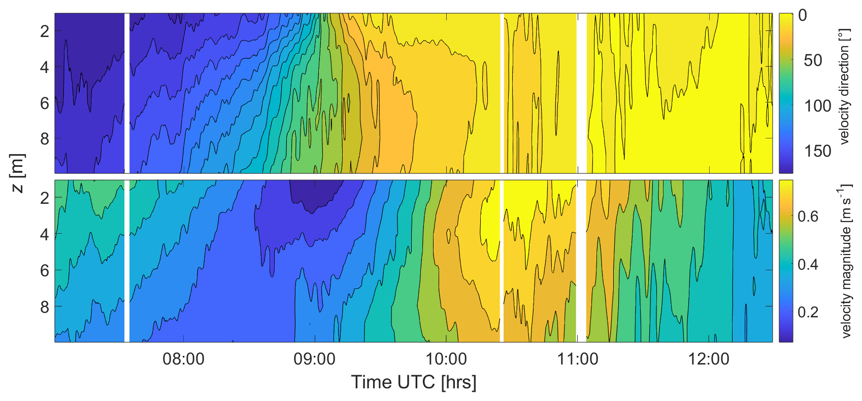
During phase I of the filament evolution in the NSL, divergence occurred around the Coriolis frequency f, with a significant convergence area between x=0.5 km and x=1.5 km (Fig. 6d). Over depth, the convergence core extended from 4 m at x≈ 1 km down to 8 m at x=1.5 km. Dense water sank along the density gradient (Fig. 6a) at $\sim \mathrm{15}\mathrm{m}{\mathrm{d}}^{-\mathrm{1}}$ (Fig. 6j), accumulating beneath lighter water (Fig. D1). This downwelling also dragged light water downward at about half the magnitude of w. Below the convergence zone, divergence developed alongside anticyclonic vorticity for x>1 km and cyclonic vorticity for x<1 km, both within the Rossby radius (Fig. 6g; Thomas et al., 2008), producing uplift of the filament flanks at $\sim \mathrm{12}\mathrm{m}{\mathrm{d}}^{-\mathrm{1}}$. CTD profiles (Fig. D1) confirmed dense bottom water being advected upward into shallower layers by divergence flow. These ASC signals correspond to a reversed pattern of low-density filamentogenesis (i.e., filamentolysis) characterized by downwelling in the core and uplift on the flanks.

In phase II, as divergence increased, the convergence core contracted vertically by ∼2–3 m and horizontally by ∼0.25 km within 17 min (Fig. 6e). The steep density gradients relaxed through mixing, reducing downward motion (Fig. 6k), while CTD profiles showed flattening isopycnals at $z=\mathrm{100}cm.$ Anticyclonic divergence expanded toward the surface on the right boundary (Fig. 6e and h), driving upwelling up to 20 m d⁻¹ (Fig. 6k) and exporting dense water laterally away from the filament. Vertical shear in the along-front velocity (Fig. 6k) was additionally higher on the right side of the filament, potentially causing advection or enhanced stirring. The general increase in along-front velocity over throughout t1–t3 may be due to the late phase of low tide. There, the flood current already sets in in the bottom layer, while the ebb current still flows at the surface (Fig. E1). This tidal asymmetry develops due to the freshwater contrasts between the surface and lower layers, causing upwelling near the sea floor. Overall, phase II represented a transitional regime: the downwelling of phase I largely disappeared, but the complete boundary downwelling characteristic of filamentogenesis had not yet emerged. Instead, ASC signatures combined remnants of filamentolysis with early signs of filamentogenesis, suggesting that the main circulation had already shifted upward into the overlying first meter.

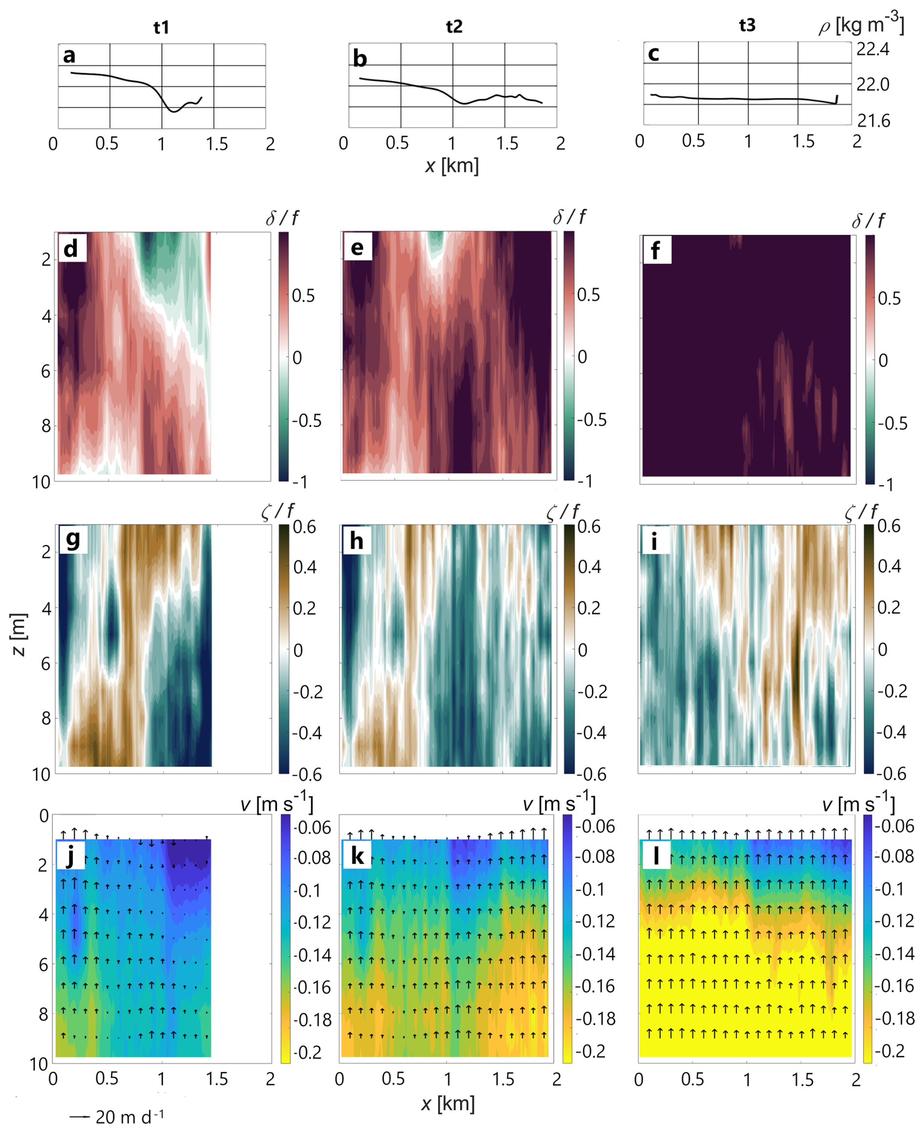
Figure 6 Sections of low-density filament kinematics. (a–c) Density profile over distance from ASV CTD data at z=100 cm for [$t\mathrm{1}=\mathrm{07}:\mathrm{23}$ am, $t\mathrm{2}=\mathrm{07}:\mathrm{40}$ am and $t\mathrm{3}=\mathrm{08}:\mathrm{30}$] UTC on 5 August in the NSL. Underlying panels show corresponding sections over depth of normalized (d–f) δ, (g–i) ζ and (j–l) along-front velocity with overlying w (arrows) referenced to 20 m d⁻¹.

By phase III, the kinematics below 1 m revealed only the tails of the process. The density at z=100 cm dropped by $\sim \mathrm{0.3}\mathrm{kg}{\mathrm{m}}^{-\mathrm{3}}$ on the left side (Fig. 6c), consistent with vertical CTD profiles. During the final 40 min, the anticyclonic patch doubled in magnitude and extended through the full water column (Fig. 6i), while a cyclonic patch developed at x<1.5 km, inducing upwelling toward the frontal axis. The stronger cyclonic upwelling displaced the convergence core at x=1 km, replacing it with lateral advection of dense water toward the low-density filament. Unlike in phase II, where ASC signals were mixed and transitional, phase III was marked by intensified divergence and upwelling, pointing to the fact that true filamentogenesis had now strengthened above 1 m. This interpretation is supported by the restratification of isopycnals at 0.6 m in the ASV CTD data (Fig. 5) and the drifter observations at 0.5 m, which captured the surface expression of filamentogenesis that the ADCP could only detect indirectly.

Taken together, the ASC patterns evolved from reversed circulation in phase I (filamentolysis), through a transitional mixture in phase II, to enhanced filamentogenesis above 1 m in phase III, with only its residual upwelling detectable below. This sequence reflects the canonical circulation patterns of low-density filamentogenesis (McWilliams et al., 2015; Jakes et al., 2024), but with the unique distinction that salinity rather than temperature, dominated the gradients driving filament evolution. Furthermore, the observe patterns show an asymmetry, where the right side of the filament was prone to different local kinematics than the left side of it. Importantly, the ASC observations add a dynamic perspective to the restratification processes already identified in the sensor chain, drifter, and ASV CTD datasets, confirming that the filament's uplift was a coherent, cross-dataset signal in the upper water column.

4 Discussion

The synoptic-Lagrangian in situ observations in this study show a narrow, low-density filament that formed due to freshwater-driven buoyancy and was embedded in a tidal mixing front that showed a distinctive response to the tidal flow. Filaments store potential energy and act to capture the kinetic energy of waves, tides, and currents (Thomas et al., 2008), mainly when biofilms occur at convergence zones and the wave-dumping effect is visible (Wurl et al., 2016). The filament established in the lower and overlying first meter of the NSL (Figs. 2 and 4), features strong surface convergence guided by same-order divergence, suggesting the development of an ASC (Fig. 5; McWilliams et al., 2015) that may favor the exchange of gases, nutrients (from biofilms), heat and, energy between the ocean surface, deeper layers and the atmosphere. Taking this interaction potential as motivation, the goal of this section is to understand the evolution of filamentary structure and flow in a highly dynamic regime in the near-surface layer of the ocean.

a. Evidence and structure of the low-density filament

The observations provide robust evidence for the occurrence of a low-density filament embedded in a tidal mixing front in the southern North Sea. Signals of uplift, convergence, and buoyancy production were consistently detected across all independent datasets. The sensor chain captured the filament during flood as a sharp density contrast driven by freshwater contrasts and buoyancy signal relative to the surrounding waters. It also confirmed that the filament formed on the light side of the tidal mixing front, as isopycnal characteristics and stratification shifted markedly during the front crossing under the combined influence of southeasterly winds and the tidal ebb wave. Drifters independently captured the filament through trajectory diffraction and associated divergence-convergence patterns at its boundaries. ASV CTD transects during ebb revealed the filament as an even sharper horizontal density gradient within the uppermost meter, although the right filament border could not be fully resolved due to the transect length. ADCP profiles complemented these results by recording a full convergence signal across the filament, extending approximately 0.8 km horizontally and 4–8 m vertically. The repeated detection of the filament during both ebb and high tide underscores that it was a genuine tidal mixing front feature rather than a tidal current artifact. Furthermore, in all data sets an asymmetry in filament structure occurred, with the right border of the filament being eroded stronger than the left side over time.

Unlike dense filaments, which tend to form recurrently and persist over longer periods (McWilliams et al., 2009; Chrysagi et al., 2021; Garcia-Jove et al., 2022), low-density filaments are said to appear far more volatile. The observed low-density filament depended highly on freshwater-driven buoyancy and tidal redistribution, which continuously reshape near-surface density gradients. Their buoyant positioning at the very top of the water column likely impact this fragility, since atmospheric forcing and tidal stirring act directly on the gradients that sustain them. Importantly, the gradients here were salinity-driven, in clear contrast to the temperature-driven dense filaments that dominate open-ocean settings (Mahadevan and Tandon, 2006; McWilliams et al., 2015; Jakes et al., 2026). This salinity control represents a unique pathway for filamentogenesis, potentially characteristic of shelf and estuarine systems such as the North Sea.

b. ASC patterns in the overlying first meter and lower NSL

The ASV CTD and ADCP measurements together provide a coherent view of filament ASC patterns, revealing three distinct phases that unfolded over the short span of one hour. This rapid timescale may explain the scarce observations of low-density filaments and the inherent difficulty of capturing their dynamics in the field. However, high-resolution multi-sensor and -platform measurements help observing these processes as shown in this study.

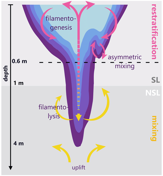
In Phase I, the filament exhibited a sharp horizontal density gradient and a cone-like structure as Jakes et al. (2024) schematized. Yet the associated ASC in the NSL >1 m, however, showed rather a filamentolysis pattern with downwelling occurring within the core and uplift at the flanks. Upwelling from the near-bottom was induced by tidal modulation (see section c.) and along-front vertical velocity shear advecting density gradients differentially (Johnson et al., 2020). The vertical shear arises from the already propagating flood current in the bottom layer, while the ebb current still persists at the surface (Burchard and Badewien, 2015; Stanev et al., 2014) and might be a fuelled by down-front wind in the direction of the surface frontal jet, slowing down velocities in the upper and enhancing mixing in the lower NSL (Mahadevan and Tandon, 2006; Thomas et al., 2008). This instability acted to erode the filament, setting the stage for subsequent transitions in phases II and III.

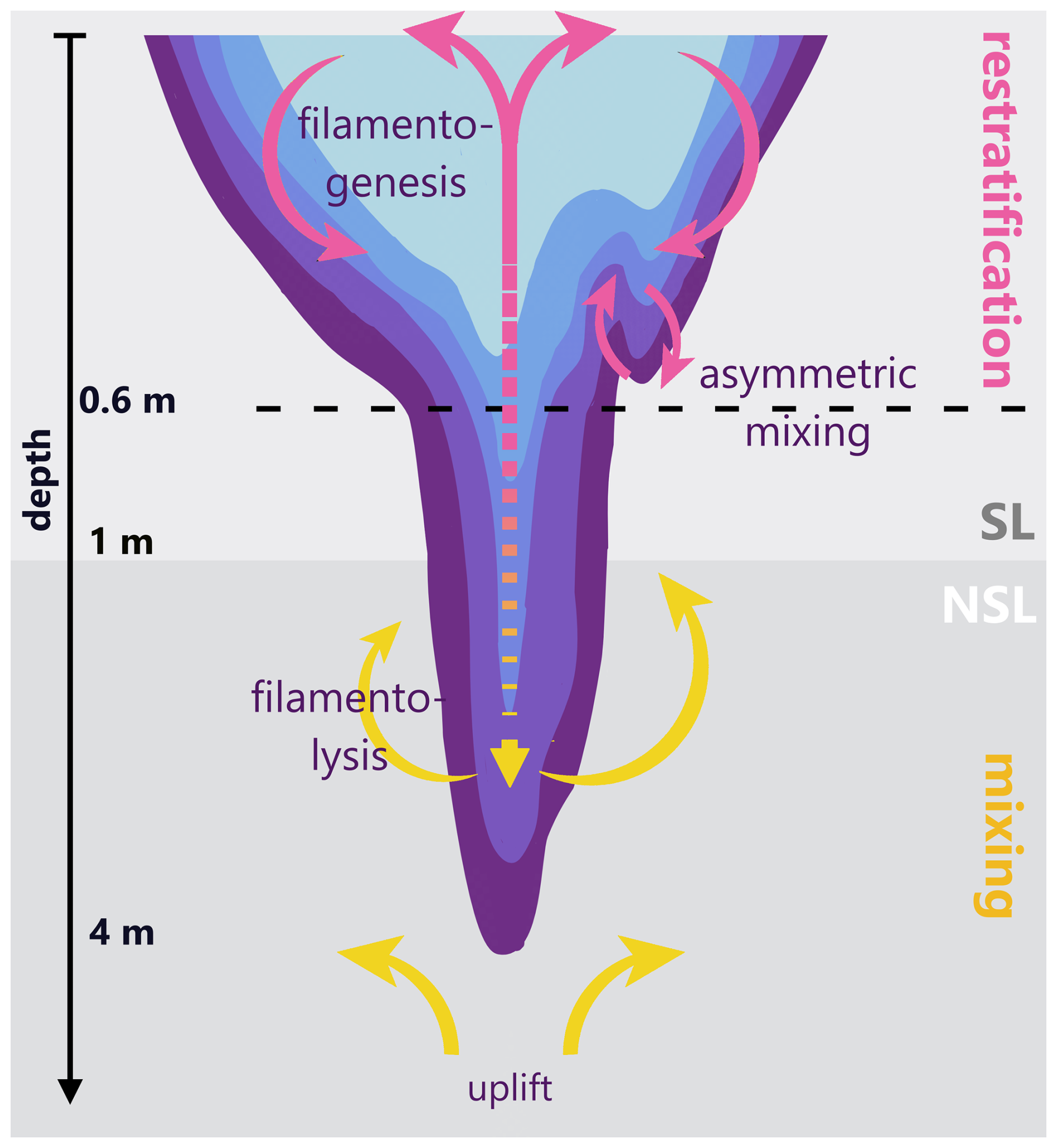
Figure 7 Schematic process of filamentolysis-induced filamentogensis in the NSL. ASC associated with upper-NSL filamentogenesis (restratification) is colored pink, ASC associated with lower-NSL filamentolysis (mixing) is yellow.

In Phase II (Fig. 7), downwelling in the lower NSL weakened due to the decrease in density gradient strength, while signals of upwelling and divergence intensified. This intensification, however, caused spatially asymmetric erosion, with earlier and stronger weakening on the eastern/right-hand side of the filament. This asymmetry coincides with evolving kinematic conditions, including a gradual reduction of convergent signatures in $\mathit{\delta }/f$, increasingly patchy anticyclonic vorticity, and a broadening of the secondary circulation. In addition, across-front velocity sections show stronger near-surface across-filament flow and enhanced horizontal and vertical shear on the eastern side, suggesting locally intensified differential advection or lateral stirring, both vertically and horizontally. Above 0.6 m, early restratification established with flattening of isopycnals on both boundaries of the filament core, indicating downwelling, pointing toward potential filamentogenesis of a low-density filament in the upcoming 40 min. The loss of buoyancy in the lower layer, therefore, fueled buoyancy production in the upper NSL, resulting in a two-layer coupled filamentolysis-filamentogenesis process.

In Phase III, these signatures intensified further: divergence broadened, upwelling strengthened, so that below 1 m the filament completely vanished from the water column. In the upper 0.6 m, restratification is fully established.

A snapshot of the filamentogenesis pattern indicated by isopycnals, hinting toward upwelling in the core and downwelling at the flanks, was only captured in the upper 1 m (drifters, ASV CTD). Below 1 m, ADCP observations alone were insufficient to resolve the full pattern, recording only the lower NSL filamentolysis. This highlights the importance of simultaneous, co-located ASV CTD and ADCP measurements for resolving the vertical structure of ASC in the NSL and for disentangling the coupling of submesoscale processes across layers.

c. Tidal modulation of filament formation and vertical velocities

The observed ASC patterns were strongly modulated by tides, which both enhanced and suppressed filamentary circulation depending on phase. Drifter data reveal that acceleration of the tidal flow induced divergence and upwelling, whereas deceleration toward low water produced convergence and downwelling. Due to the temporal offset between ASV and drifter deployments, the time series of drifter data was too short to resolve the coupling of tides with the filament at ebb tide. However, together with the data from the sensor chain, the tidal modulation of the filament could be resolved during high tide.

Within the simplified tidal-modulation framework based on Copernicus SSH-derived divergence (Sect. 3.2), decelerating ebb flow would generally be expected to enhance convergence and support downward motion within the filament. However, the observations do not clearly reflect this expected strengthening of convergence. One possible contributing factor may be a vertical phase structure in the tidal circulation, where flood flow already intrudes the lower water column while ebb current still propagate near the surface. In such a configuration, the expected convergent tendency may potentially weakened by upwelling caused by the underneath accelerating flood current or local filament upwelling. Constructive and destructive interference between tidal motions and filament-induced circulation may have further modulated vertical velocities, contributing to the observed reduction in filament coherence, as also reflected in the sensor chain signal (Sect. 3.1). Overall, the filament appears to have evolved within a kinematically heterogeneous environment where evolving patchy anticyclonic vorticity and local shear structures likely modulated the background tidal convergence field. Given the simplified nature of the tidal-modulation estimate and the limited spatial resolution of the forcing fields, the relative contributions of tidal forcing, vertical phase structure, and local advection processes remain difficult to fully disentangle, but together they provide a consistent qualitative framework for the observed asymmetric erosion.

Quantitatively, divergence values at the observed tidal mixing front reached 1–4 times higher than those reported in the Alboran Sea (Rypina et al., 2021; Garcia-Jove, 2022; Esposito et al., 2023) or the Bay of Bengal (Essink et al., 2022). While these exaggerated magnitudes may partly reflect overestimation by the area-based drifter method due to rapid tidal deformation of drifter triplets, they nonetheless point to strong tide-filament interactions. The resulting vertical velocities reached up to 50 m d⁻¹ during divergence phases and down to -40 m d⁻¹ during convergence phases. Comparisons between methods further highlight the tidal imprint, so that drifter-based estimates were roughly twice as large as ADCP-derived velocities, but converged to similar magnitudes once tidal displacement at the surface is removed from the drifter calculations.

d. Implications for surface exchange and heat uptake

Once filamentogenesis was established in the upper meter, the system became more efficient at absorbing heat, with uptake doubling despite only weak net temperature changes. This enhanced capacity highlights the importance of low-density filaments as effective, short-lived hotspots of exchange at the ocean–atmosphere interface. Tidal modulation, salinity redistribution and rapid phase transitions may make them mediators of vertical exchange. While dense filaments dominate in the open ocean, low-density filaments may represent a likely important, yet less frequent, pathway for near-surface fluxes in shelf and estuarine seas.

5 Conclusion and outlook

The study provides multi-dataset observation of a low-density filament on the submesoscale [O(0.1–10 m)] driven by freshwater-driven buoyancy embedded and modulated within a tidal mixing front. By combining complementary datasets from sensor chains, drifters, ASV CTD transects, and ADCP profiles, a coherent sequence of filament alteration and associated ageostrophic secondary circulation (ASC) was identified that unfolded on timescales of approximately one hour. The three observed phases point toward the coexistence of filamentolysis in the deeper near-surface layer and filamentogenesis confined to the upper meter, revealing a tightly coupled, layer-dependent response that could only be captured through multi-instrument, high-resolution observations.

Unlike the dense, temperature-driven filaments commonly described in the open ocean, the low-density filament observed here was associated with strong freshwater-driven buoyancy contrasts, highlighting a distinct estuarine pathway to filament formation. The observations further suggest that tidal modulation strongly influenced the filament structure and surface divergence patterns, with different tidal phases associated with amplification or weakening of the frontal signal. This tidal influence may also contribute to local filament processes such as the asymmetric erosion of filament flanks and the transition from strong lateral buoyancy gradients toward restratification. Restratification during filamentogenesis coincided with enhanced surface warming, suggesting a potential link between submesoscale circulation and upper-ocean heat storage. Our observations further indicate that freshwater-driven buoyancy contrasts play a central role in filament formation, while tidal modulation can amplify or weaken the surface divergence signal depending on tidal phase. However, the use of sea surface height for the estimation of tidal modulation of the divergence budget only provides a simplified model that is restricted to the surface. Since dense North Sea water and less dense water mixed with freshwater originating from rivers such as Elbe and Weser create a vertical tidal phase shift, it is crucial to also incorporate tidal modulation in the deeper layers. Further, more synoptic spatial and temporal assessments are necessary to resolve the background and tidal flow accompanying the filament. These results thus are a first approach in coupling freshwater-driven buoyancy and tidal impact on a how low-density filament that may contribute to vertical exchange and air–sea coupling in the ocean. More broadly, resolving the transient dynamics of buoyancy-driven filaments and their tidal modulation may improve our understanding of upper-ocean stratification and regional climate feedbacks.

Taken together, the results expand the current paradigm of filament dynamics by demonstrating a salinity-driven mechanism for coupled low-density filamentogenesis and -lysis in shelf seas. Future work should quantify the frequency of such features in estuarine and coastal systems and assess their role in larger-scale balances of heat, gas exchange, and energy. To advance this, improved synoptic measurement strategies are needed, featuring congruent CTD and ADCP deployments that allow filamentary structure and ASC to be described more quantitatively, for instance, through frontal tendency calculations.

Appendix A

Since horizontal divergence is used to diagnose vertical motion, the vertical velocity in the water column can be determined. Restructuring the continuity equation $\frac{\partial u}{\partial x}+\frac{\partial v}{\partial y}+\frac{\partial w}{\partial z}=\mathrm{0}$ results in

$$\begin{array}{}\text{(A1)}& \begin{array}{rl}{\displaystyle }\mathrm{\Delta }w& {\displaystyle }=-{\int }_{-z}^{z^{\mathrm{0}}}\left({\displaystyle \frac{\mathrm{d}u}{\mathrm{d}x}}+{\displaystyle \frac{\mathrm{d}v}{\mathrm{d}y}}\right)\mathrm{d}z\\ {\displaystyle }\leftrightarrow w\left(z_i\right)-w\left(z_{i-\mathrm{1}}\right)& {\displaystyle }={\int }_{z_i}^{z_{i-\mathrm{1}}}{\displaystyle \frac{\mathrm{d}u}{\mathrm{d}x}}\mathrm{d}z\\ {\displaystyle }& {\displaystyle }={\left[\left({\displaystyle \frac{\mathrm{d}u}{\mathrm{d}x}}+{\displaystyle \frac{\mathrm{d}v}{\mathrm{d}y}}\right)z\right]}_{z_i}^{z_{i-\mathrm{1}}}\\ {\displaystyle }& {\displaystyle }=\left({\displaystyle \frac{\mathrm{d}u}{\mathrm{d}x}}+{\displaystyle \frac{\mathrm{d}v}{\mathrm{d}y}}\right)z_{i-\mathrm{1}}-\left({\displaystyle \frac{\mathrm{d}u}{\mathrm{d}x}}+{\displaystyle \frac{\mathrm{d}v}{\mathrm{d}y}}\right)z_i\\ {\displaystyle }& {\displaystyle }=\left({\displaystyle \frac{\mathrm{d}u}{\mathrm{d}x}}+{\displaystyle \frac{\mathrm{d}v}{\mathrm{d}y}}\right)(z_{i-\mathrm{1}}-z_i)\\ {\displaystyle }w\left(z_i\right)& {\displaystyle }=w\left(z_{i-\mathrm{1}}\right)+\left({\displaystyle \frac{\mathrm{d}u}{\mathrm{d}x}}+{\displaystyle \frac{\mathrm{d}v}{\mathrm{d}y}}\right)\mathrm{\Delta }z,\end{array}\end{array}$$

where w(z_i) is the vertical velocity in the target depth z_i, w(z_i−1) is the vertical velocity in the previous depth z_i−1 and Δz is the difference between neighboring depths. For w(z_i−1) of the drifters, the SSH (Fig. A1) is obtained from model data (CMEMS, 2024) to emulate the vertical velocity that arrives from the tidal wave

$$\begin{array}{}\text{(A2)}& w\left(z_{i-\mathrm{1}}\right)={\displaystyle \frac{\mathrm{1}}{n}}{\sum }_{k=\mathrm{1}}^n{\text{SSH}}_k\cdot {\displaystyle \frac{\mathrm{1}}{\mathrm{\Delta }t}},\end{array}$$

where SSH_k is the tidal amplitude and Δt=1 h is the temporal resolution of the model data. Thus, w(z_i−1) will be applied to Eq. (5) as hourly mean with a standard deviation of ±0.3 m resulting in an error $\mathrm{\Delta }w\left(z_{i-\mathrm{1}}\right)\approx \mathrm{7}\mathrm{m}{\mathrm{d}}^{-\mathrm{1}}$.

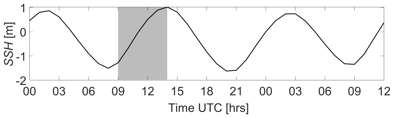
Figure A1 Hourly mean SSH obtained from model data (CMEMS, 2024) for the drifter deployments. The observation time of the filament is shaded in grey.

Appendix B

The correlation of model SSS (CMEMS, 2024) with salinity recorded by a Ferrybox flow-through system is shown in Fig. B1. For each spatial bin of the model data at a time step, Ferrybox salinity data is averaged within that bin and at that specific time. Proceeding like this for the three consecutive days (4–6 August), the resulting data points are plotted for standard deviation, time, latitude and longitude. Applying a linear regression to the correlation, a R² of 0.705 can be achieved. The standard deviation throughout the correlation data lies on average below 0.05 g kg⁻¹ and reaches only in a few exceptions 0.1–0.15 g kg⁻¹ that are not covered by the regression. Regarding the temporal distribution, especially the slack water times from late 4 August and whole 5 August fall out of the regression. In terms of latitude, those outliers are mostly pronounced in higher latitudes (>54.2° N) and for longitude in eastward values (>8.1° E). The model data, thus, underestimates the salinity in the eastern, more coastal areas, probably assuming a higher freshwater input and hence a lower salinity than was obtained by the Ferrybox. In particular during low water, when the ebb current exports the more saline water seawards, the model predicts a lower reduced salinity. Compared to this, in more western areas, in between the slack water times, the estimation of the model is much better.

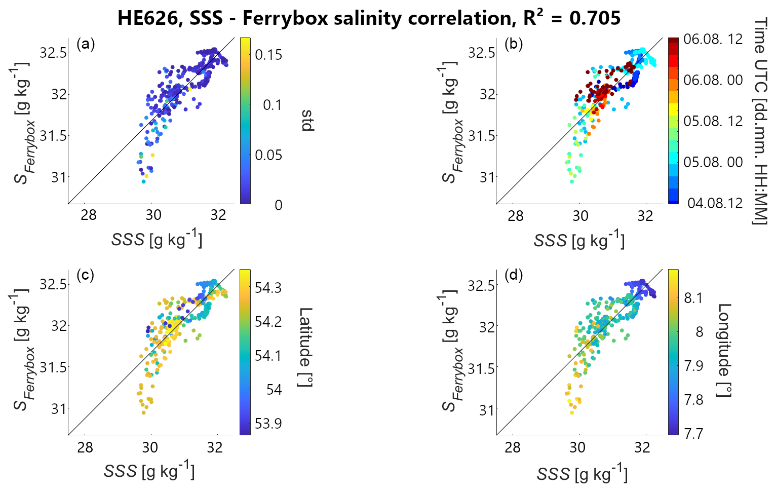
Figure B1 Correlation of SSS from model data (CMEMS, 2024) and Ferrybox salinity regarding (a) salinity standard deviation, (b) time (UTC), (c) latitude and (d) longitude. The linear regression model results in a correlation of R²≈0.71.

Appendix C

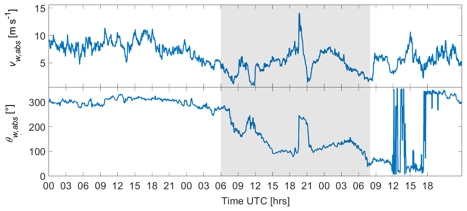
Figure C1 (top) Absolute wind speed v_w,abs and (bottom) wind direction at 10 m θ_w,abs during the survey obtained from the weather station on RV Heincke. The grey shaded area highlights the period of the filament measurements.

Appendix D

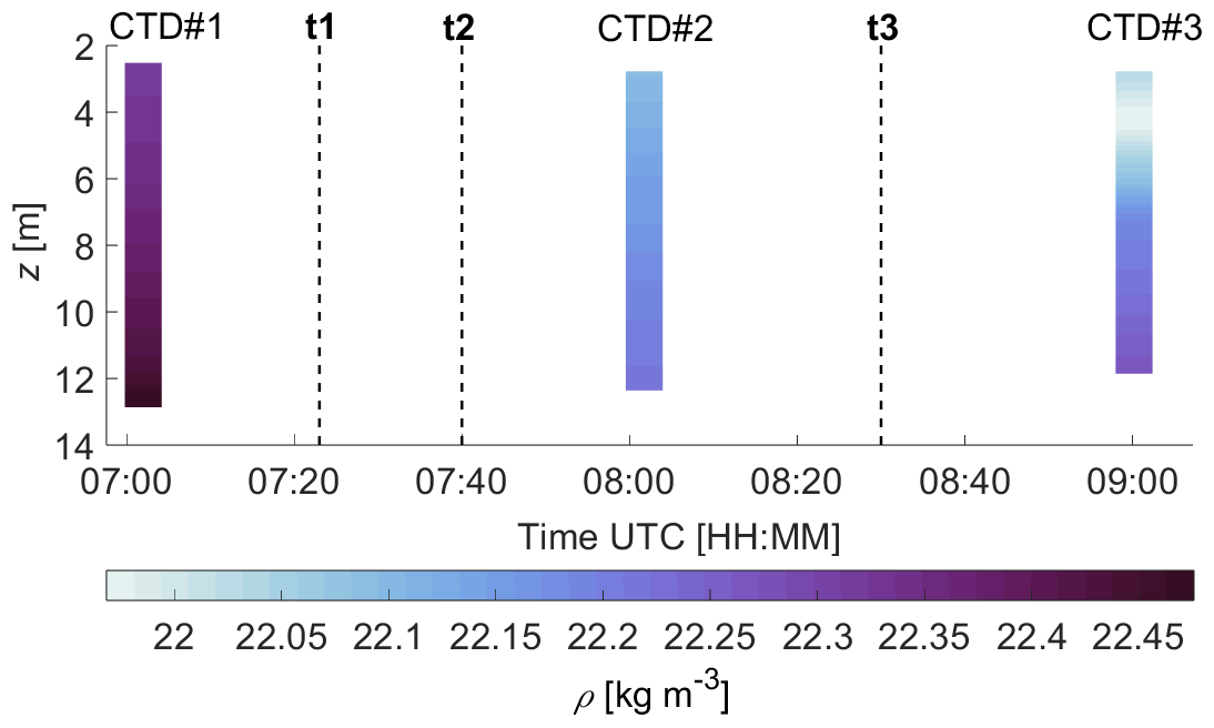
Figure D1 Vertical profiles of density from ship CTD during the observation period. Sections t1–t3 from the filament analysis of the ASV data (Sects. 3.3 and 3.4) are marked as vertical dashed lines.

Appendix E

Figure E1 Contour of velocity magnitude and direction for 5 August over time and depth.