Wave-induced sediment resuspension potential in the Finnish Archipelago, Baltic Sea: integrating field measurements with large-scale numerical model simulations

Sediment resuspension, driven by wind-wave-induced shear stress, is a key process influencing coastal water quality, biogeochemical cycles, and the transport of pollutants and organisms. The critical shear stress, τ_cr, is a central parameter in sediment transport models, since initiation of motion can occur when wave-induced shear stress exceeds the critical value. In this study, we implemented a high-resolution (20 m) spectral wave model to simulate near-bottom orbital velocities across the complex archipelago of southwestern Finland. We then used laboratory measurements from in situ sediment samples to determine a model for the critical shear stress that accounts for physical properties using the median grain size and the dry bulk density, and the time-varying biological variation using chlorophyll a. Our proposed model, ${\mathit{\tau }}_{\mathrm{cr}}\left(d_{\mathrm{50}},{\mathit{\rho }}_{\mathrm{B}},\mathrm{Chl}a\left(t\right)\right)$, explained 66 % of the variation of the measured critical shear stress for our data collected from three different sediment types (Mud, Sand and Mixed sediments). The modelled mean critical shear stress differed between sediment classes, with values of 0.49 N m⁻² for Mud, 1.56 N m⁻² for Sand, and 1.02 N m⁻² for Mixed sediments. The variability in the critical shear stress around the mean values driven by a non-constant biological contribution was approximately 30 % for Mud and Sand, and approximately 50 % for Mixed sediments. Finally, we used a class-level map of the sea floor and the in situ grain size data to translate the wave model orbital velocities to near-bottom shear stresses. Based on the numerical model data, the critical shear stresses from the newly proposed model, ${\mathit{\tau }}_{\mathrm{cr}}(d_{\mathrm{50}},{\mathit{\rho }}_{\mathrm{B}},\mathrm{Chl}a(t\left)\right)$, were rarely exceeded based on only wave-induced motions in most of the model grid, but could, nonetheless, be exceeded to up around 10 % of the times in smaller areas. This study highlights the importance of incorporating both physical and biological factors – and their temporal dynamics – into sediment transport models to achieve reliable predictions of critical shear stresses and resuspension potential.

1 Introduction

Sediment resuspension is a key process in shallow coastal environments, influencing water quality, nutrient dynamics, and overall ecosystem health (Edge et al., 2015; Green and Coco, 2014). Resuspension can release contaminants and nutrients from sediments, increase turbidity, and redistribute sediment particles, thereby affecting biogeochemical cycles, primary production, seabed morphology, and benthic habitats (Heiskanen, 1998; Green and Coco, 2014). The potential for sediment resuspension depends on the balance between the forces acting on the sediment bed and the sediment's resistance to motion.

In coastal areas, resuspension dynamics are primarily driven by wind waves and currents, which exert shear stress τ (N m⁻²) on the seabed. The initiation of particle movement from the sediment surface is governed by the critical shear stress (τ_cr). When the applied shear stress on the seabed exceeds this threshold, sediment particles can be lifted into the water column – a process known as resuspension (Shields, 1936; Soulsby and Whitehouse, 1997). In shallow waters where currents are typically weak, wave-induced shear stress is the dominant driver of sediment resuspension (Pascolo et al., 2018).

Critical shear stress depends on sediment properties, including grain size, bulk density, water content, and chlorophyll a and organic matter content (Grabowski et al., 2011). Grain size is a fundamental determinant of erodibility, but in fine sediments, cohesive forces – driven by electrochemical and biological interactions – become increasingly important (Black et al., 2002; Roberts et al., 1998). Biological factors further modify sediment stability: benthic fauna influence porosity and sediment structure through bioturbation and feeding activities (Mulsow et al., 1998; Michaud et al., 2006; Harris et al., 2015), while vegetation dampens hydrodynamic forces and stabilizes sediments via root systems (Koch et al., 2007; Madsen et al., 2001).

Consequently, critical shear stress and resuspension potential vary across space and time (Joensuu et al., 2018, 2020). Although sediment transport models often estimate critical shear stress from median grain size (d₅₀) (Dade et al., 1992), natural sediments exhibit substantial variability (Grabowski et al., 2011). Seasonal biofilm formation by microphytobenthos can increase τ_cr by up to fourfold (Le Hir et al., 2007; Decho, 2000). Despite this complexity, sediment transport models often estimate τ_cr solely from median grain size (Dade et al., 1992), ignoring biological and seasonal variability, although a recent modelling study by Zhang et al. (2025) incorporated seasonal values of τ_cr.

To improve predictions of sediment resuspension potential, we integrate empirical data (Joensuu et al., 2018, 2020) into our modelling approach. Our objectives are: (i) to use high-resolution wave simulations to map spatial variability in near-bottom shear stress, (ii) to develop a spatial and temporal seabed model integrating in situ data to estimate critical shear stress, and (iii) to estimate sediment resuspension potential probabilities based on model outputs.

Our study area is located in the Hanko archipelago on the northern coast and entrance of the Gulf of Finland, the Baltic Sea (Fig. 1). This region provides an optimal setting for investigating sediment resuspension processes as it is characterized by a mosaic of islands with a diverse range of coastal habitats that capture the spatial variability in seabed composition and in the physical and biological factors regulating sediment erodibility and resuspension dynamics.

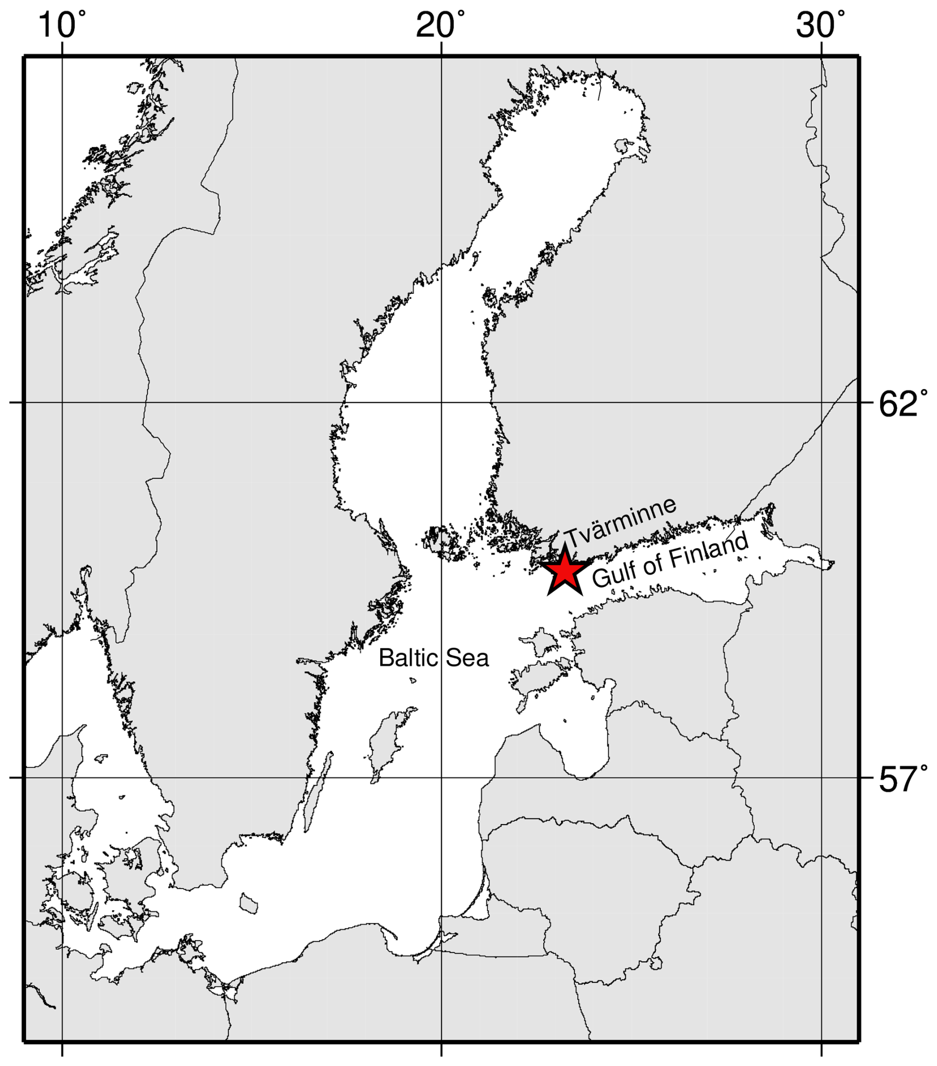
Figure 1 Location of the Tvärminne research station in the western Gulf of Finland, Baltic Sea.

The Baltic Sea is a semi-enclosed, brackish, and shallow sea, with a mean depth of 54 m and negligible tidal currents. In the study area, bottom currents are generally weak, ranging from a few centimetres per second to a maximum of 10 cm s⁻¹ under typical conditions (Westerlund et al., 2018). However, current speed can exceed 10 cm s⁻¹ occasionally in narrow channels or during upwelling events (Westerlund et al., 2018; Miettunen, 2024). Consequently, sediment resuspension is predominantly governed by wind-wave induced shear stresses. Prevailing winds are from the southwest, with an average speed of 7–8 m s⁻¹ (Alenius et al., 1998).

2 Wave data

2.1 Wave observations

Wave conditions were observed near Tvärminne research station in March and April 2017 using two Datawell Directional Waverider buoys: a larger 90 cm Mk-III at 24 m depth (outer archipelago) and a smaller 40 cm DWR-G4 at 17 m depth (inner archipelago) (Datawell, 2025). Both buoys were located about 3 km east of the Tvärminne research station (Fig. 2).

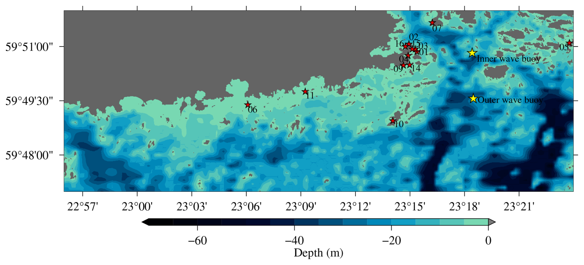
Figure 2 The bottom topography, in situ sediment sampling stations (01–16, marked by red stars), and wave buoy locations (yellow stars) are shown.

Both wave buoys sampled at a frequency of 1.28 Hz and calculated the wave spectrum up to 0.58 Hz. Low-frequency data below 0.05 Hz were discarded when calculating wave parameters. These observations were used to validate the numerical wave model.

2.2 Wave simulations (SWAN)

The SWAN model (Booij et al., 1999) is a spectral wave model that was developed especially for shallow water and nearshore simulations. We implemented SWAN for 1 August–30 September 2014 to catch the spatially extensive sediment measurement campaign (Joensuu et al., 2018), for 1 May–30 November 2015 to cover the temporally extensive sediment measurement campaign (Joensuu et al., 2020), and 1 March–30 April 2017 to cover the period of the wave measurements (for validation purposes). Simulations were forced by data from a numerical FMI-HIRLAM weather prediction system (e.g. Eerola, 2013), where the wind speed and direction had been processed to a height of 10 m. The wind data had a spatial resolution of roughly 7.4 km, and a 1 h temporal resolution for the years 2014, 2015, and 3 h for 2017.

The model was implemented to a 0.01 nmi (∼ 20 m) regular grid with lateral boundary conditions taken from a 1 nmi Baltic Sea wide SWAN simulation using the same wind forcing. A 0.01 nmi resolution is finer than what is typically used in wave models, but SWAN has been implemented on a similar resolution before in the Baltic Sea (Alari and Raudsepp, 2012). Another spectral model has also been implemented on the North-American coast with an adaptive resolution as fine as 10 m (Abdolali et al., 2020). The available bathymetric data has been composed of data from nautical charts and the VELMU depth model (https://ckan.ymparisto.fi/dataset/velmu-syvyysmalli, last access: 29 June 2026) by the Finnish Environment Institute (SYKE) and had a resolution of 0.1 nmi. The land–sea mask has been rasterized based on a polygon dataset from SYKE (https://ckan.ymparisto.fi/dataset/ranta10-rantaviiva-1-10-000, last access: 22 June 2026) and was available at a 0.01 nmi resolution. Land points were edited to wet points in the 0.1 nmi bathymetrical grid using the surrounding depth information. Additional depth information from Joensuu et al. (2018), Valanko (2012), and field sampling were used. The final 0.1 nmi grid was bi-linearly interpolated to a resolution of 0.01 nmi and the land-sea mask was applied (Fig. 2).

The wave model produced direct hourly gridded estimates of the maximum near-bottom orbital velocity, U_bot (m s⁻¹), and the near-bottom mean periods, $T_{{\mathrm{m}}_{\mathrm{bot}}}$ (s). The near-bottom amplitudes, a_bot (m), were determined directly by the velocity and period estimates. For a full definition of the wave parameters, see Appendix A.

During the simulation periods, the modelled prevailing wave direction at the outer wave buoy was around 225°, and all waves with a height of 2 m or over came from direction between 175 and 225°. The highest significant wave height of 2.9 m was during a wave event from 195° with mean wave periods ($T_{{\mathrm{m}}_{\mathrm{01}}}$) up to 5.8 s. The simulation period also captured high waves (up to 1.7 m) from the east (95°), although these were less frequent. This distribution aligns with the dominant directions observed in the Gulf of Finland (Pettersson et al., 2010). Statistics of the modelled near-bottom velocities can be found in Appendix B.

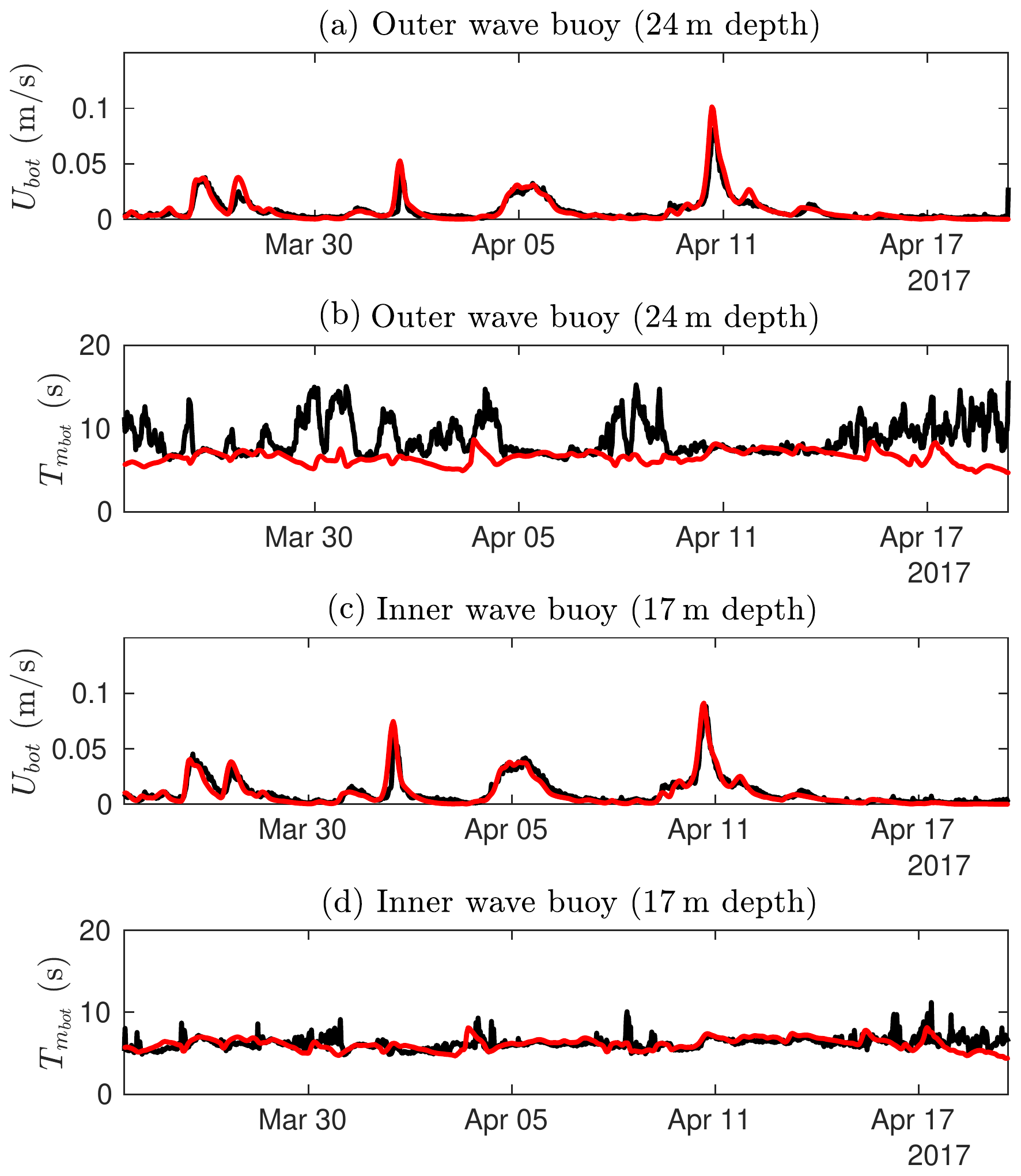
Figure 3 Wave-induced near-bottom orbital velocities and wave period calculated by the SWAN model (red) and from the wave spectra measured by wave buoys (black). The long near-bottom wave periods during calm conditions in (b) are due to noise in the measurements, see Sect. 2.2 for details.

We validated the modelled near-bottom orbital velocities and wave periods by determining them from the measured wave spectrum using the same water depth as in the bathymetrical grid used in SWAN. Near-bottom velocities were modelled accurately at both locations (Fig. 3a, c) with the more exposed outer location showing a −0.04 cm s⁻¹ bias and 0.47 cm s⁻¹ root-mean-square-error (RMSE). The slightly shallower inner location had a 0.08 cm s⁻¹ bias and 0.49 cm s⁻¹ RMSE. Modelled near-bottom periods (Fig. 3b, d) agreed well at the inner location with a 0.12 s bias and 0.88 s RMSE. For the outer location, bias was 2.23 s and RMSE 3.31 s, reflecting deeper water where wave orbital motions do not reach the bottom and the period is determined by low-frequency noise in the measurements. As seen in Fig. 3b, near-bottom periods were well modelled during high near-bottom velocities, but less defined under calm conditions. The validation of bulk surface wave parameters showing the temporal dynamics and scatter are shown on Figs. C1 and C2 in Appendix C.

The wave model SWAN has been extensively used and verified in the Baltic Sea. In the open sea areas, the accuracy of the model was found good (e.g. Björkqvist et al., 2018; Giudici et al., 2023). Closer to the shore, and especially in the archipelago in the northern parts of the Baltic Sea, the accuracy of the numerical wave models depends on the grid size, reflecting the capability of the model to resolve smaller islands and variable bottom topography that influence the wave energy dissipation (e.g. Tuomi et al., 2014). A detailed analysis of the performance of three different numerical wave models, including SWAN, in the archipelago off Helsinki in the Gulf of Finland showed that the models on 0.1 nmi grid resolution are capable of simulating the wave field with good accuracy (Björkqvist et al., 2020). In the present study, our grid resolution is 20 m, and the islands and bottom topography are well resolved as the comparison with measurements show (Appendix C and Fig. 3). The validation period in 2017 did not include the highest sea states during the study periods in 2014 and 2015, but according to the studies mentioned above, also the high wind events can be expected to be reasonably well simulated.

2.3 Wave-induced shear stress, τ_w

The near-bottom shear stress was computed as (e.g. Soulsby, 1997):

$$\begin{array}{}\text{(1)}& {\mathit{\tau }}_{\mathrm{w}}=\mathrm{0.5}{\mathit{\rho }}_{\mathrm{w}}{f}_{\mathrm{w}}{U}_{\mathrm{bot}}^{\mathrm{2}},\end{array}$$

where ρ_w=1003 kg m⁻³ is the water density and f_w is the wave friction coefficient. The friction coefficient was determined following Soulsby (1997) as the larger of the rough and smooth bottom estimates:

$$\begin{array}{}\text{(2)}& f_{\mathrm{w}}=max\mathit{\{}{f}_{\mathrm{wr}},f_{\mathrm{ws}}\mathit{\}},\end{array}$$

where

$$\begin{array}{}\text{(3)}& f_{\mathrm{wr}}=\mathrm{0.237}{r}^{-\mathrm{0.52}},\end{array}$$

is the rough bottom friction coefficient, $r=a_{\mathrm{bot}}/k_{\mathrm{s}}$, k_s=2.5d₅₀ is the Nikuradse equivalent sand grain roughness, and

$$\begin{array}{}\text{(4)}& f_{\mathrm{ws}}=B{R}_{\mathrm{w}}^{-N}\end{array}$$

is the smooth bottom friction coefficient. Here $R_{\mathrm{w}}=U_{\mathrm{bot}}{a}_{\mathrm{bot}}/\mathit{\nu }$ is the Reynolds number, ν is the kinematic viscosity of water ($\mathrm{1.3}\times {\mathrm{10}}^{-\mathrm{6}}$ m² s⁻¹), a_bot is the amplitude of the wave-induced near-bottom velocities (see Appendix A for a definition), and B and N are constants that depend on the Reynolds number such that:

$$\begin{array}{}\text{(5)}& {\displaystyle }B=\mathrm{2},N=\mathrm{0.5}\mathrm{for}{R}_{\mathrm{w}}\le \mathrm{5}\times {\mathrm{10}}^{\mathrm{5}}\left(\mathrm{laminar}\right)\text{(6)}& {\displaystyle }B=\mathrm{0.0521},N=\mathrm{0.187}\mathrm{for}{R}_{\mathrm{w}}>\mathrm{5}\times {\mathrm{10}}^{\mathrm{5}}\left(\mathrm{turbulent}\right)\end{array}$$

3 Environmental data and seabed classification

3.1 Environmental data

Environmental data and critical shear stress measurements were available from two field campaigns conducted in the years 2014 (Joensuu et al., 2018) and 2015 (Joensuu et al., 2020) in the Hanko archipelago. In 2014, samples were gathered from 16 shallow sites (depth < 4 m), covering a sedimentary gradient from mud to sand (median grain sizes 21–570 µm). These sampling locations are illustrated in Fig. 2. The 2014 field campaign focused on spatial variation in sediment erodibility, maximizing variation in sediment surface characteristics (e.g. bedforms, biofilms) across sites. In 2015, three sites (mud (ID04), mixed (ID09), and sandy (ID14) sediment) from the 2014 study were re-sampled from April to December to capture temporal variation in sediment erodibility. In this campaign, variation in sediment characteristics was minimized to focus solely on temporal changes.

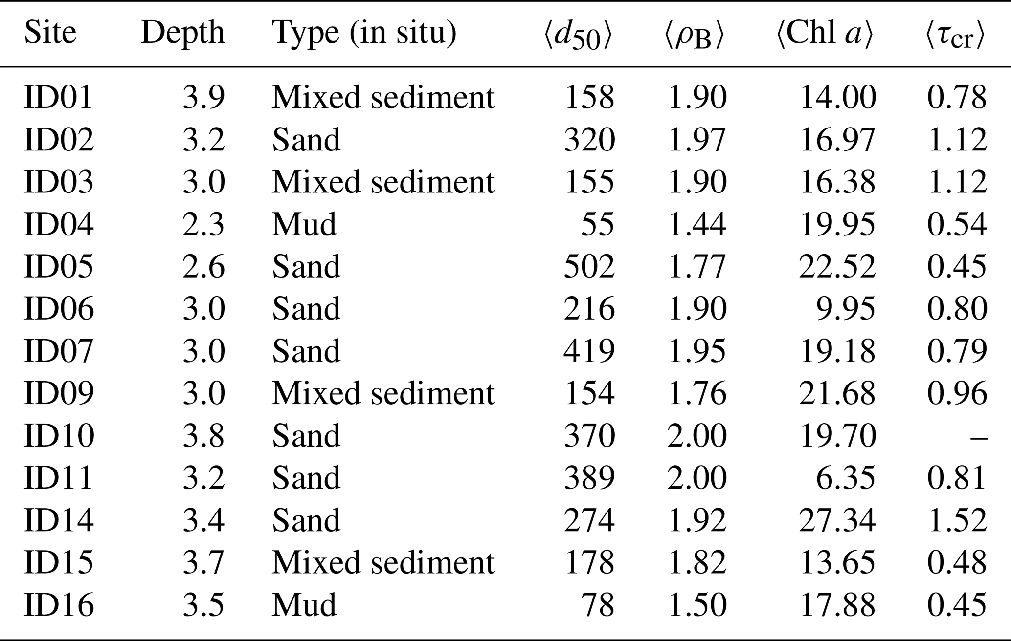
The sampling procedure was consistent across both campaigns. At each site, SCUBA divers collected samples by carefully inserting EROMES cores (10 cm diameter, 10 cm depth) into the sediment (Schünemann and Kühl, 1991). Samples were maintained at in situ temperatures and transported to the laboratory for further measurements. A total of 59 and 73 EROMES cores were collected in 2014 and 2015, respectively. For a detailed description of the sampling procedures, see Joensuu et al. (2018, 2020). The grain size, dry bulk density and chlorophyll a for each measurement site were determined from the combined 2014 and 2015 data as mean of monthly means (Table 1).

Table 1 The depth (m), median grain size d₅₀ (µm), dry bulk density ρ_B (g cm⁻³), Chlorophyll a Chl a (µg g⁻¹) and critical shear stresses, τ_cr (N m⁻²) based on the in situ measurements. 〈〉 denotes averages, which have been calculated as means of monthly means.

3.2 Measurements of critical shear stresses, ${\widehat{\mathit{\tau }}}_{\mathrm{cr}}$

In the 2014 and 2015 field campaigns (Joensuu et al., 2018, 2020), the critical shear stresses from the sediment samples were determined in the laboratory with a portable EROMES device (Schünemann and Kühl, 1991; Andersen, 2001). Bed shear stress on the sediment surface is generated by turbulent fluctuations induced by a propeller and baffle ring. The baffle ring prevents rotational flow and ensures turbulent flow fluctuations mimicking those observed by waves in nature. Suspended solids concentration was monitored with an OBS sensor (optical back-scattering sensor). The propeller revolutions were calibrated to nominal bed shear stresses (Schünemann and Kühl, 1991; Andersen, 2001).

At each run, the bed shear stress was increased every 2 min by 0.1 N m⁻² from 0 to 2.0 N m⁻² in the year 2014 study and from 0 to 1.6 N m⁻² in the year 2015 study. Water samples for gravimetric analysis were collected during each run to calibrate the OBS sensor into suspended solids concentration (SSC; mg L⁻¹) (Andersen, 2001; Andersen and Pejrup, 2002). The critical shear stress (N m⁻²) was defined at the erosion rate of 0.1 (g m⁻² s⁻¹), which describes the erosion after the erosion of unconsolidated “fluffy” material (Andersen, 2001; Andersen et al., 2005). For a more extensive description of the laboratory procedures, see Joensuu et al. (2018, 2020).

Since the EROMES device is not reliable for large grain sizes, we excluded individual critical shear stress measurements when the median grain size of the sample exceeded 300 µm. Consequently, no reliable measurements were obtained from site ID10 (Table 1).

3.3 Class-based seabed model

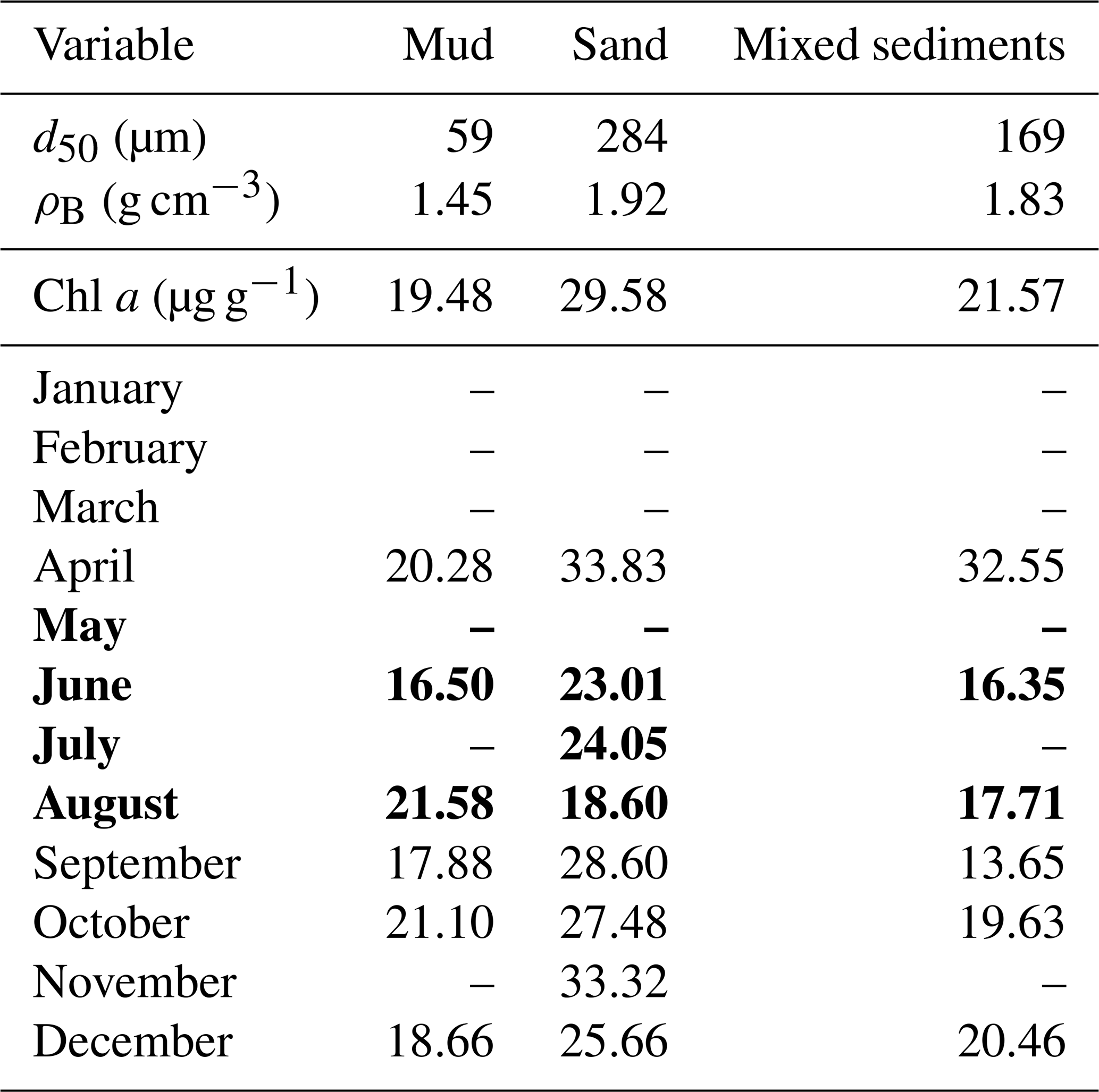
We used EMODnet Seabed Substrates (1 : 100 000) (Kaskela et al., 2019) to define seabed classes: Mud to muddy sand, Sand, Mixed sediments, Coarse sediments, and Boulders (see Fig. 4a). Coarse sediments and Boulders were excluded from this study, since we had no in situ data from those seabed types. For Mud, Sand, and Mixed sediments we determined representative median grain sizes for each seabed type based on the data from Sect. 3.1 (Table 2). The representative values were determined as means of monthly means to not give too much weight to data from the spatial campaign.

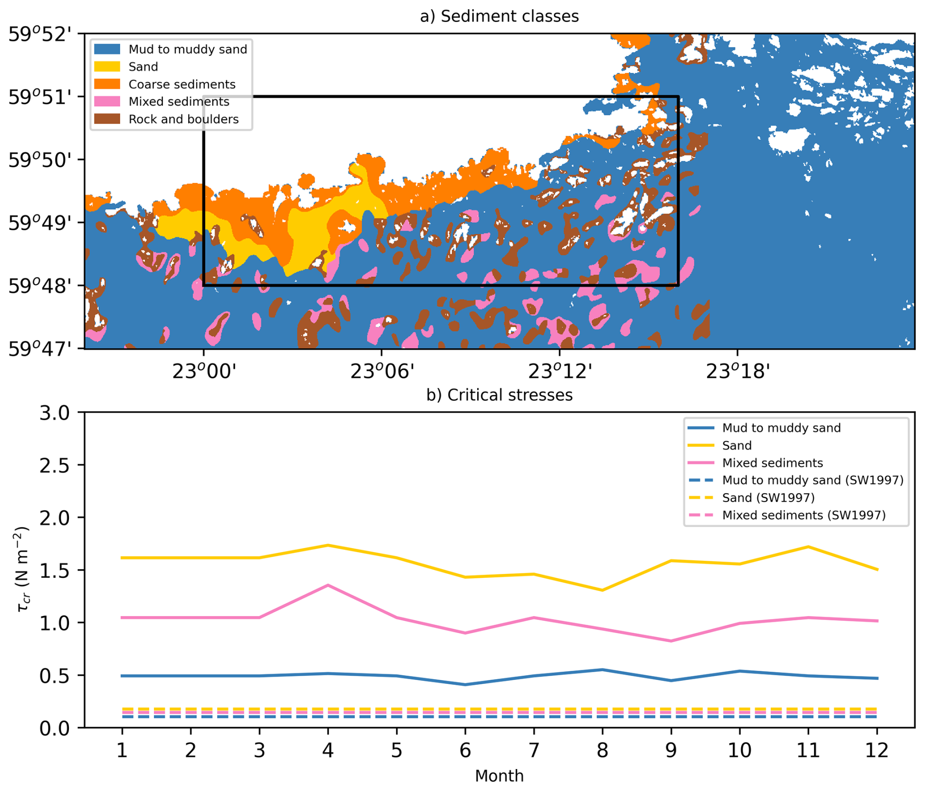
Figure 4 The sediment classes from the EMODnet data (a) and the critical shear stresses estimated based on the time varying model (Eq. 10) and the d₅₀ model of Soulsby and Whitehouse (1997) (Eq. 7) (b). The black rectangle in (a) is the area shown in Figs. 6–9.

Table 2 Representative physical properties for each sediment class used in the model. The values for chlorophyll a is an average outside the growth season (growth season marked in bold), and is used if there is no month-specific value available.

4 Models for critical shear stresses, τ_cr

4.1 Soulsby and Whitehouse (1997)

The critical shear stress is the threshold shear stress above which particle motion is initiated. The critical shear stress depends on the sea floor properties, and is given by

$$\begin{array}{}\text{(7)}& {\mathit{\tau }}_{\mathrm{cr}}={\mathit{\theta }}_{\mathrm{cr}}({\mathit{\rho }}_{\mathrm{s}}-{\mathit{\rho }}_{\mathrm{w}})g{d}_{\mathrm{50}}\end{array}$$

where τ_cr (N m⁻²) is the critical shear stress, θ_cr is the threshold Shields parameter, g is the gravitational acceleration (9.82 m s⁻²), ρ_s is particle density (2650 kg m⁻³), ρ_w is the water density (1003 kg m⁻³) and d₅₀ is median grain size (m) (Soulsby, 1997).

The parametrization of the Shields parameter, as improved by Soulsby and Whitehouse (1997), reads:

$$\begin{array}{}\text{(8)}& {\mathit{\theta }}_{\mathrm{cr}}={\displaystyle \frac{\mathrm{0.3}}{\mathrm{1}+\mathrm{1.2}{D}_{*}}}+\mathrm{0.055}\left[\mathrm{1}-{\exp }^{\left(-\mathrm{0.02}{D}_{*}\right)}\right]\end{array}$$

where D_* is the dimensionless grain size calculated with

$$\begin{array}{}\text{(9)}& D_{*}={\left({\displaystyle \frac{g(\frac{{\mathit{\rho }}_{\mathrm{s}}}{{\mathit{\rho }}_{\mathrm{w}}}-\mathrm{1})}{{\mathit{\nu }}^{\mathrm{2}}}}\right)}^{\frac{\mathrm{1}}{\mathrm{3}}}{d}_{\mathrm{50}}.\end{array}$$

The strength of this model is its simplicity, but we found it to result in estimates of the critical shear stress that were an order of magnitude too small compared to values determined in the laboratory from in situ samples (Fig. 4b).

4.2 Thompson et al. (2019)

Thompson et al. (2019) developed predictive models for critical shear stress based on physical and biological characteristics in the Celtic Sea and North Sea. Their approach combined principal component analysis (PCA) and multiple linear regression, identifying key predictors such as median grain size, sorting, kurtosis, percentage of fines, bulk density, porosity, chlorophyll a, and organic carbon. Two models were proposed:

• Model 1 (Celtic Sea): Included both physical and biological parameters, suggesting that bed stability increases with grain size, better sorting, and greater bulk density, while decreasing with greater proportions of fines and organic carbon.

• Model 2 (North Sea): Relied on physical parameters only, but over-predicted bed strength when applied to Celtic Sea data.

These models demonstrated that physical characteristics dominate bed stability, while biological factors (e.g. chlorophyll a) play a secondary role. However, they also highlighted the complexity and co-variation of sediment properties, making broad-scale predictions challenging without site-specific data.

These models were not applicable in our study for several reasons. First, we lacked key parameters such as grain sorting and kurtosis, and organic carbon content, which are essential for Model 1. Second, the model had a negative coefficient for dry bulk density despite Fig. 3 of Thompson et al. (2019) showing a positive relationship between bulk density and bed stability. This negative coefficient combined with bulk densities being higher in our data compared to the dataset of Thompson et al. (2019), resulted in unphysical values of the critical shear stress. Finally, their models were calibrated for Celtic and North Sea conditions, which differ from our study area in water depth, sediment composition, hydrodynamic forcing, and shear stress history.

4.3 A non-stationary physical–biological model

We constructed a parsimonious model that couples time-invariant physical factors – median grain size (d₅₀, µm) and dry bulk density (ρ_B, g cm⁻³) – with a time-varying biological proxy, chlorophyll a (Chl a, µg g⁻¹). To fit the model we returned to the raw in situ measurements reported by Joensuu et al. (2018, 2020). Since EROMES measurements are not reliable for very coarse sands, samples with d₅₀>300 µm were excluded.

The final dataset used for the new regression model contained n = 108 individual observations covering the three sediment classes. The model was determined as a three variable least-squares fit using the individual samples from the raw data. In other words, the model predicts critical shear stress as:

$$\begin{array}{}\text{(10)}& {\mathit{\tau }}_{\mathrm{cr}}={\mathit{\beta }}_{\mathrm{0}}+{\mathit{\beta }}_{\mathrm{1}}{d}_{\mathrm{50}}+{\mathit{\beta }}_{\mathrm{2}}{\mathit{\rho }}_{\mathrm{B}}+{\mathit{\beta }}_{\mathrm{3}}\mathrm{Chl}a\end{array}$$

where τ_cr is critical shear stress (N m⁻²), β₀ is the intercept, d₅₀ is median grain size (µm), ρ_B is dry bulk density (g cm⁻³), and Chl a is chlorophyll a (µg g⁻¹).

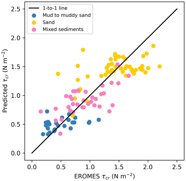
The fit made to each sediment class (Sand, Mud, Mixed sediments) separately had only modest predictive power, whereas the combined model (using all observations) explained a substantially larger portion of the variance (R²=0.659, p≤0.01) (Table 3, Fig. 5). The RMSE of the full model was 0.31 N m⁻². Importantly, the combined fit captures the differences between the classes more efficiently than the class-specific models (Table 3). Since the primary purpose of the model is to provide class-level critical shear stress estimates for application to the seabed classes (Sect. 3.3), this ability of the model to reproduce the variation between classes is more relevant than its performance within individual classes.

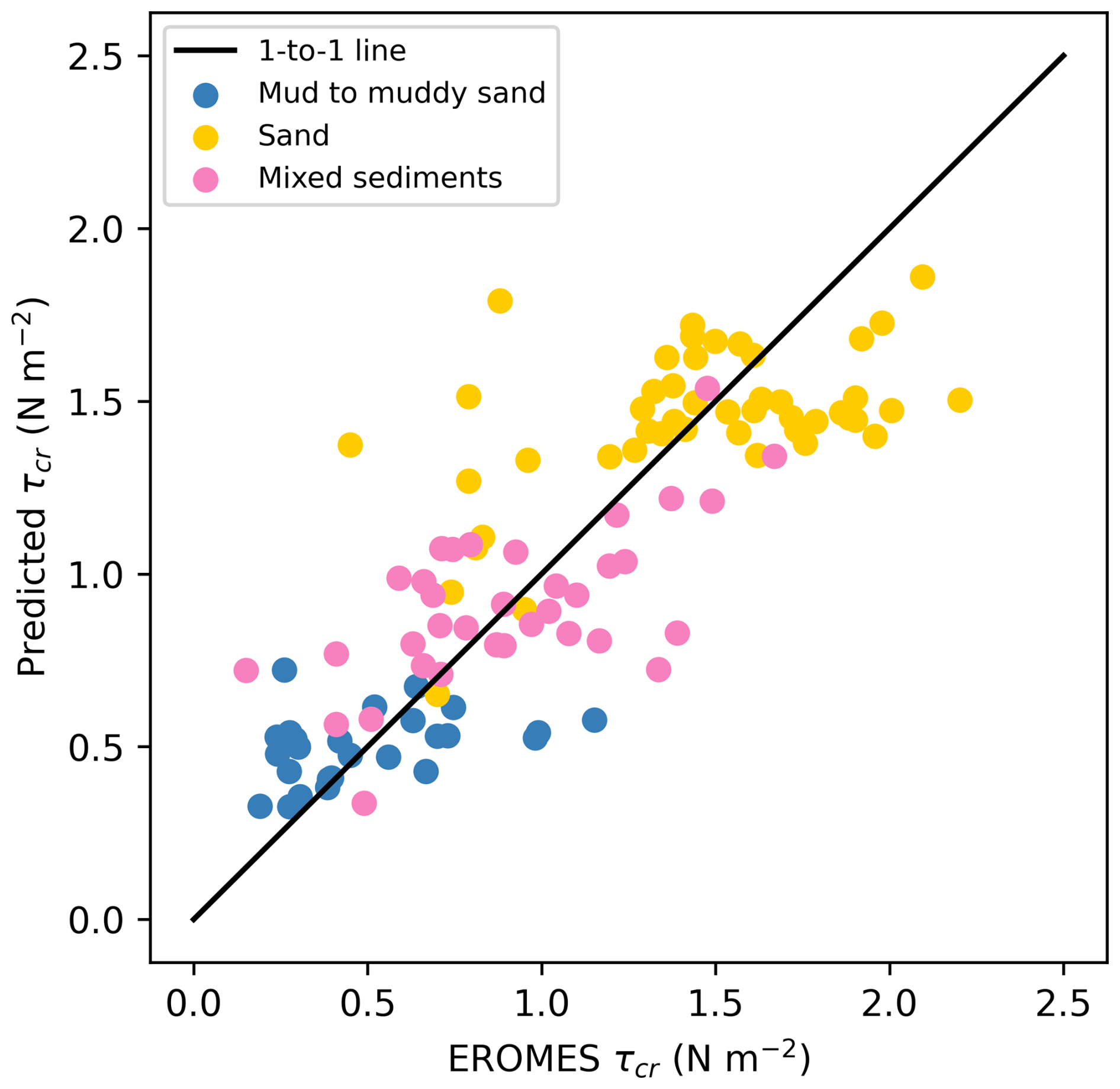
Figure 5 The critical shear stresses determined with the EROMES device from in situ samples compared to the critical stresses predicted using d₅₀, ρ_B and Chl a (Eq. 10).

Table 3 Multiple linear regression models for the critical shear stress ${\mathit{\tau }}_{\mathrm{cr}}={\mathit{\beta }}_{\mathrm{0}}+{\mathit{\beta }}_{\mathrm{1}}{d}_{\mathrm{50}}+{\mathit{\beta }}_{\mathrm{2}}{\mathit{\rho }}_{\mathrm{B}}+{\mathit{\beta }}_{\mathrm{3}}\mathrm{Chl}a$ (Eq. 10) based on the in situ data from Joensuu et al. (2018, 2020). For each sediment class, the regression coefficients, coefficient of determination (R²), p-value, root-mean-square error (RMSE; N m⁻²) and number of observations (n) are shown. The combined model using all sediment types (shown in bold) has the strongest predictive power and is the model applied in this study.

ns – not significant.

We assessed collinearity among the predictors used in the combined model (n=108) by examining pairwise Pearson correlations and variance inflation factors (VIF) following the protocol of Zuur et al. (2010). The two physical variables were strongly correlated (R=0.86 between d₅₀ and ρ_B), reflecting their expected co-variation in natural sediments, whereas Chl a showed only weak correlations with the physical variables (R=0.10 and R=0.34). VIF values indicated moderate collinearity for the physical variables (VIF${}_{d_{\mathrm{50}}}=\mathrm{4.96}$, VIF${}_{{\mathit{\rho }}_{\mathrm{B}}}=\mathrm{4.44}$) and low collinearity for Chl a (VIF = 1.33). Despite the moderate collinearity between the d₅₀ and ρ_B, omitting either variable from the combined model reduced the explained variance R², confirming that each physical variable contributes unique predictive information and should be retained.

Physical variables explained most of the variation in τ_cr, but including chlorophyll a increased the explained variance (R²) by approximately 0.1.

Our aim was not to build the most comprehensive model for the τ_cr but to define a practical model that can be combined with numerical wave model outputs. To use the modelled critical shear stresses with the spatio–temporal wave model data, we determined representative values of d₅₀ and ρ_B for each of the three classes (Mud, Sand, and Mixed sediments), and monthly values of Chl a for each of the classes. The model is not applied to coarse sediments or boulders because representative values cannot be reliably determined from the available data.

The raw data from the in situ samples were therefore grouped according to the determined seabed classes: $\mathrm{Mud}=\mathit{\{}\mathrm{ID}\mathrm{04},\mathrm{ID}\mathrm{16}\mathit{\}}$, $\mathrm{Sand}=\mathit{\{}\mathrm{ID}\mathrm{02},\mathrm{ID}\mathrm{05},\mathrm{ID}\mathrm{06},\mathrm{ID}\mathrm{07},\mathrm{ID}\mathrm{10},\mathrm{ID}\mathrm{11},\mathrm{ID}\mathrm{14}\mathit{\}}$ and $\mathrm{Mixed}=\mathit{\{}\mathrm{ID}\mathrm{01},\mathrm{ID}\mathrm{03},\mathrm{ID}\mathrm{09},\mathrm{ID}\mathrm{15}\mathit{\}}$ (see Table 1). For each site, monthly means were computed while retaining the year (e.g. 6–29 August 2014 and 25–27 August 2015 remain distinct) to avoid overweighting data from the spatial campaign. For d₅₀ and ρ_B, class-level monthly means were computed and then averaged to obtain time-invariant values (Table 2). For Chl a, temporal variability was retained by computing monthly means for each class. Months lacking measurements were filled with the off-season mean (September–April).

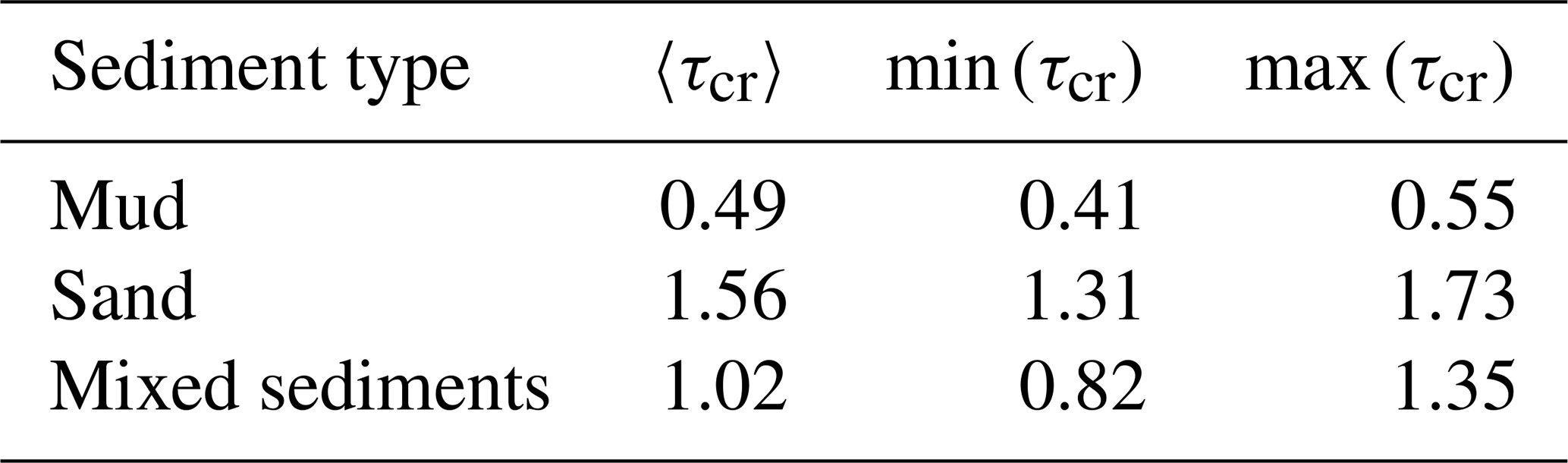
The physical variables (d₅₀ and ρ_B) define the overall magnitude of the critical shear stress for each class, with Mud being lowest and Sand being highest (Fig. 4b). The variation caused by the monthly variations in Chl a is substantial (Table 4), being up to 52 % of the mean value for Mixed sediments, and 29 % and 27 % for Sand and Mud, respectively. Nevertheless, the monthly variation never changes the ordering between the classes.

Table 4 The critical shear stresses ${\mathit{\tau }}_{\mathrm{cr}}(d_{\mathrm{50}},{\mathit{\rho }}_{\mathrm{B}},\mathrm{Chl}a(t\left)\right)$ modelled using the non-stationary physical–biological model (Eq. 10) and the values determined from the data of Joensuu et al. (2018, 2020) (Table 2). 〈〉 denotes the average of all the monthly values.

5 Spatially extensive wave-induced shear stresses

5.1 Numerical model results

Modelled shear stresses were estimated based on the near-bottom velocities (Sect. 2.2), the representative grain sizes (Sect. 4.3), and the friction coefficients (Sect. 2.3). The shear stresses were determined for every model time step from all available data (2014, 2015 and 2017). The in situ data doesn't contain samples from categories Boulders or Coarse sediments. Therefore, no representative grain sizes could be determined, and wave-induces near-bottom stresses could not be determined. Results are therefore only given for categories Mud, Sand and Mixed sediments, while the other areas are masked out.

Mean values were generally low, remaining below 1 N m⁻² across the entire area (Fig. 6a). The 95th percentiles ranged between 0.5 and 1 N m⁻² over extensive areas, especially where the seabed was classified as sand, and exceeded 1 N m⁻² in more exposed locations (Fig. 6b). The maximum near-bottom shear stress values (Fig. 6c) shows localised peaks exceeding 2 N m⁻² along several exposed areas of the coastline. These peaks occur mainly in areas classified as mud or muddy sand (compare Figs. 4 and 6c), because these locations coincide with narrow wave-exposed channels and long fetch, where near-bottom orbital velocities are particularly high (see Fig. B1 in Appendix B). Thus, although sandy areas tend to exhibit moderately larger shear stress values, the largest instantaneous maxima occur over mud bottoms due to local wave-bathymetry interactions rather than sediment type itself. The maximum values also indicate that the area directly south-west of the Tvärminne research station is well sheltered from waves, resulting in small wave-induced near-bottom shear stresses.

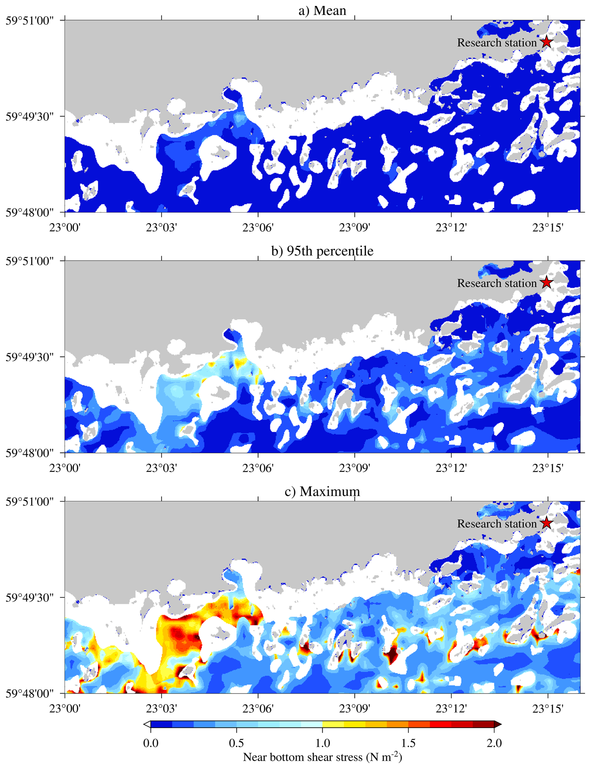
Figure 6 The mean (a), 95th percentile (b), and maximum values (c) of the modelled near-bottom shear stress covering the modelled time periods in 2014, 2015 and 2017. No results are available for classes Boulders and Coarse sediments (white), since no measurements were available from those classes to determine representative grain sizes. The red star marks the Tvärminne research station for reference.

5.2 Exceedance probabilities for critical shear stress

Modelled near-bottom shear stresses were compared to critical shear stresses to estimate erosion threshold exceedance probabilities. These probabilities reflects the likelihood that wave-induced shear stress exceeds the critical value, indicating potential sediment resuspension. Exceedance depends on wave conditions, depth, and seabed class. The critical shear stress was determined from the model in Sect. 4.3, and therefore varied monthly. Exceedance probabilities were determined simply from the fraction of times the modelled shear stress for a given time exceeded the modelled critical shear stress for the given class and month. The model is not applicable to categories Boulders and Coarse sediments, and those areas are therefore masked out.

Exceedance of the critical shear stress was generally low across the study area (Fig. 7). Localized patches in the outer archipelago exhibited exceedance of up to 10 %, indicating that sediment mobilization mostly occurs during episodic high-energy events. These areas were not limited to the coastline but also appeared among groups of islands and islets located about 2–3 km from the shoreline where the water is shallow, and include narrow channels that concentrate wave energy. Sheltered nearshore areas remained below the threshold, suggesting stable sediments and minimal resuspension potential. Even during high-wind events, modeled wave-induced shear stresses rarely exceeded predicted or measured thresholds, indicating that sediment mobilization is episodic and limited to localized areas.

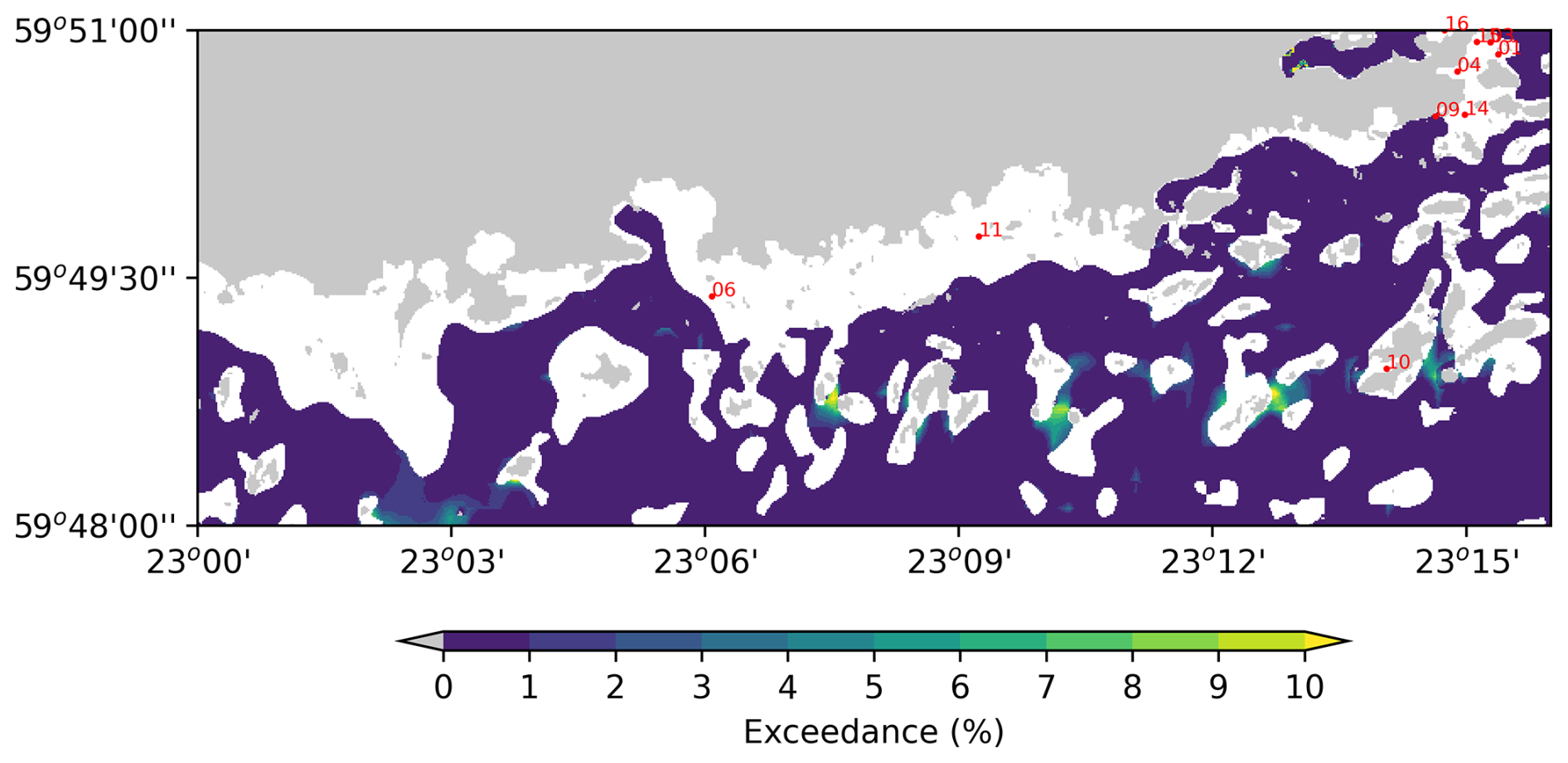
Figure 7 Percent of times the modelled shear stresses exceeded the modelled critical values during the modelled time periods in 2014, 2015 and 2017. No results are available for classes Boulders and Coarse sediments (white), since no measurements were available from those classes to determine representative values for grain size, dry bulk density and chlorophyll a.

Kahma (2021) estimated the potential for wave-induced near-bottom velocities using the long-wave (7 s) wave heights from a ray-tracing model as a proxy. The results of Kahma (2021) were 10 % exceedance values. While they are able to identify some areas that might be vulnerable to higher wave-induced near-bottom velocities, the author noted that they are not a substitute for specifically modelling the near-bottom velocities. The use of wave heights as a proxy can naturally also not account for the variation in the seabed type or the temporal variation of the critical shear stress caused by changing biological activity, as done in this study.

5.3 Wave-induced stresses during representative high-wind events

Two late-November 2015 storms illustrate the impact of strong winds on wave forcing and initiation of sediment movement. On 28 November, south-westerly winds (19–20 m s⁻¹) generated significant wave heights of ∼ 3 m offshore and ∼ 2 m within the archipelago (Fig. 8a). Near-bottom orbital velocities reached 0.5 m s⁻¹ along exposed coastlines (Fig. 8b), producing localized shear stresses exceeding 2 N m⁻² (Fig. 8c).

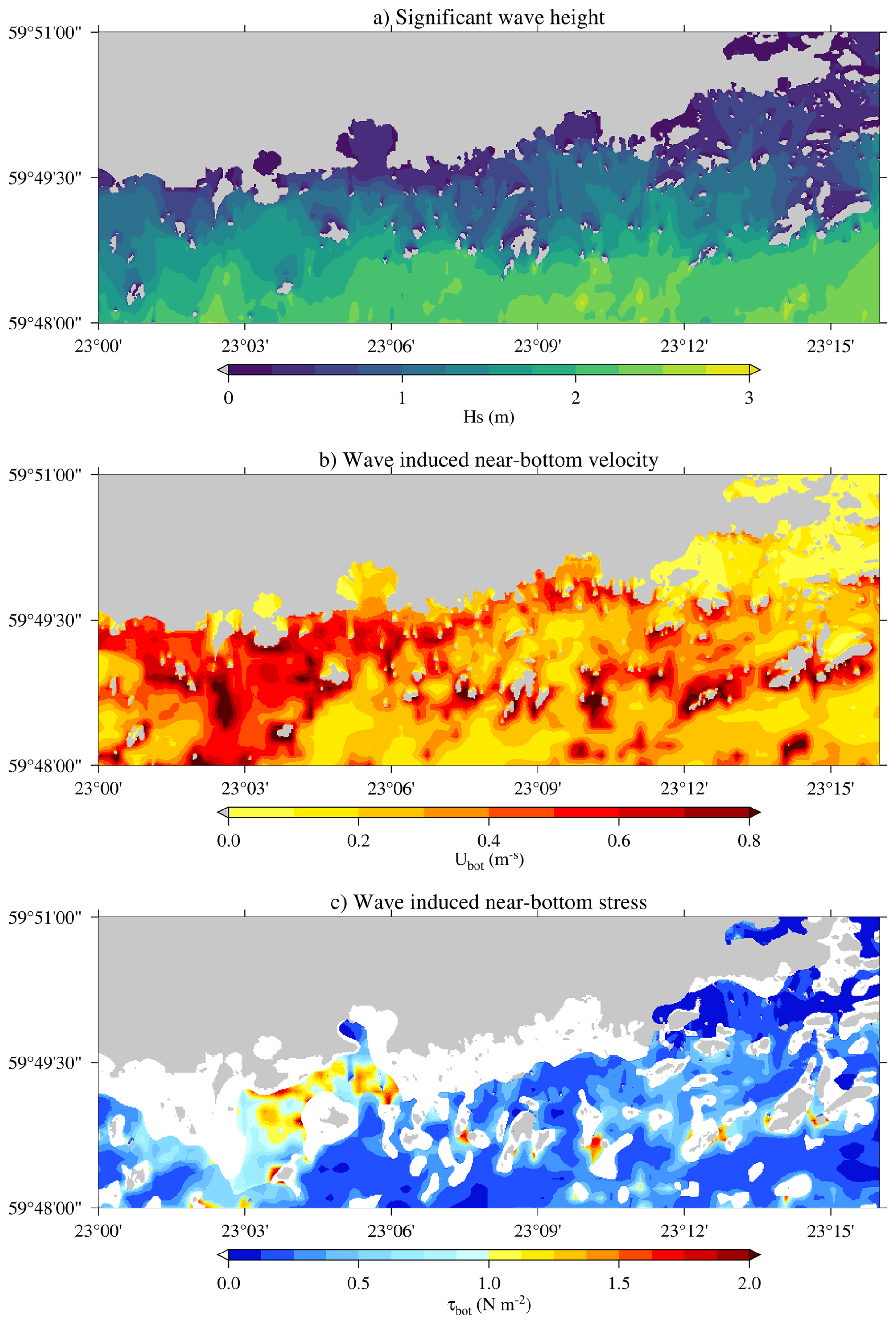
Figure 8 Wave conditions on 28 November 2015 during SW winds: (a) significant wave height, (b) near-bottom orbital velocity, (c) shear stress. Near bottom stresses are not available for classes Boulders and Coarse sediments (white), since no measurements were available from those classes to determine representative grain sizes.

The 30 November event was more severe, with SSE winds of 23–25 m s⁻¹ (gusts up to 26 m s⁻¹) causing offshore wave heights exceeding 4 m and near-bottom velocities approaching 1 m s⁻¹ in shallow exposed areas (Fig. 9b). Shear stresses surpassed 2 N m⁻² across extensive outer archipelago areas, conditions sufficient to mobilize coarse sediments (Fig. 9c).

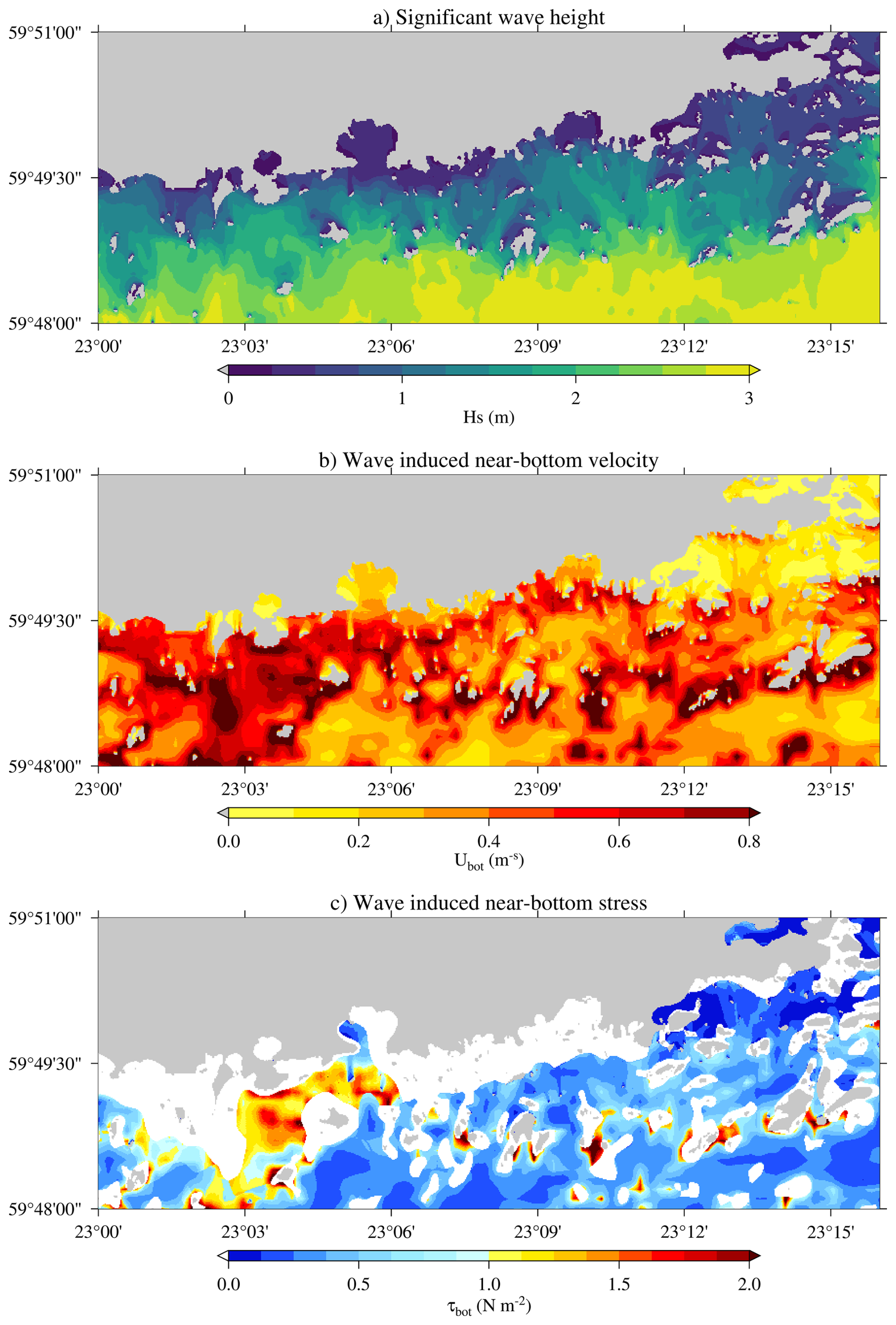
Figure 9 Wave conditions on 30 November 2015 during SSE winds: (a) significant wave height, (b) near-bottom orbital velocity, (c) shear stress. Near bottom stresses are not available for classes Boulders and Coarse sediments (white), since no measurements were available from those classes to determine representative grain sizes.

While the strongest shear stresses were mostly concentrated to the same areas in both cases, the areas with sand bottom in the western part of the area were more exposed during the SSE winds on 30 November. These two examples represent typical cases of higher waves propagating towards the shore, with south-westerly winds being the most dominant in the area. Together these two events demonstrate that sediment mobilization is highly episodic, concentrated in exposed shallow areas and constricted channels, with implications for turbidity, nutrient fluxes, and benthic habitats.

6 Discussion

The erodibility of natural sediments is influenced by a complex interplay of physical, geochemical, and biological sediment properties. For example, benthic fauna can modify sediment erodibility by altering water content, bulk density, and the particle size distribution through bioturbation activities (de Deckere et al., 2001; Le Hir et al., 2007). The experimental critical shear stresses used in this study were derived from natural submerged sediment samples, capturing variability across both space (Joensuu et al., 2018) and time (Joensuu et al., 2020). The theoretical grain-size-based thresholds following Soulsby and Whitehouse (1997) underestimated the sediment stability of the data by Joensuu et al. (2018, 2020) by roughly an order of magnitude. Indeed, previous work by e.g. Thompson et al. (2019) has shown that bulk density is an important parameter when predicting the critical shear stress, while also incorporating more detailed information about the grain size distribution (e.g. kurtosis).

Our data did not contain detailed information about the grain size distribution, so unfortunately we could not apply the models of Thompson et al. (2019) directly, but we could only assume some typical values for the missing parameters. We still found that the models of Thompson et al. (2019) were not a good description for our data. One of the main issues was that the dependence on the bulk density was negative when using multiple variables, even though the authors had found a positive dependence when using only the bulk density to describe the critical shear stresses (see their Fig. 3). It would seem like the model did not extrapolate well to the higher values of bulk density in our data. This discrepancy in sign for the coefficient might have been caused by correlations between the used variables, but we did not investigate the causes in more detail. Another reason for the weak predictive power of the model by Thompson et al. (2019) to our data might be the biological activity that can vary strongly with depth, and our data were collected in a much shallower region.

The primary limitation of grain-size-only models is their inability to account for consolidation and biological effects (Grabowski et al., 2011; van Rijn, 2020). Bulk density is a strong predictor of sediment stability: high-density sediments are more compacted and resistant to erosion, whereas low-density sediments are loose and easily mobilized (Jepsen et al., 1997; Roberts et al., 1998). Biological activity further modifies stability, especially throughout the growth season, complicating critical shear stress estimates and spatial mapping (Joensuu et al., 2018, 2020; Le Hir et al., 2007). We therefore proposed a model that addresses these limitations by incorporating bulk density and chlorophyll a as a proxy for biostabilization.

The critical shear stresses derived here represent initiation of motion rather than suspension. Suspension thresholds (e.g. van Rijn, 2020) are typically based on idealized sediment properties and do not account for biological effects or sediment heterogeneity, making them not directly comparable with EROMES-based estimates. This distinction may contribute to variability, particularly in coarser sediments, but does not affect the assessment of sediment mobilization.

We decided to build our model that relies on a few key variables for two main reasons. First, a model can only be applied if the necessary data is available. Using only three variables increases the likelihood that future datasets will contain all the required variables. Second, many of the variables correlate, and using several correlated variables further increases the uncertainty in the estimates for the individual coefficients when working with a limited data set. We chose to fit our model to three parameters: median grain size, dry bulk density and chlorophyll a. The physical aspects are covered by the grain size and bulk density, while the biology is represented by the chlorophyll a. There is no objective way to choose the variables, but these three have been used in previous models and it is expected that they might be among the variables that are more routinely measured compared to e.g. grain size distributions.

The three parameter linear model could explain most of the variation in the measured shear stresses between sediment classes (Mud, Sand, and Mixed sediments), accounting for 65.9 % of the total variance across all observations (Table 3, Fig. 5). Nonetheless, the variation of the individual critical shear stress measurements from the data within a single class were not explained equally well (Table 3). The model especially struggled with samples from a muddy seafloor, while performing better on samples classified as mixed sediments. Joensuu et al. (2020) found that, compared to the other classes, the shear stress for muddy bottoms were more heavily influenced by the biology, and we surmise that a single variable (Chl a) might not capture the biological effects well enough to sufficiently model the variations in critical shear stress on muddy seabeds. In particular, extracellular polymeric substances (EPS) produced by microphytobenthos can contribute to sediment cohesion; however, EPS measurements from the same study area showed pronounced seasonal and sediment-type variability but did not emerge as a significant explanatory variable for sediment erodibility (Joensuu et al., 2020). For this reason, EPS was not included in the present model, although it may be an important factor in other environments, such as intertidal mudflats. Nonetheless, when the aim is to spatially generalize the measurements with only class-based maps, each class can only be represented by a single value. It is therefore most critical that the model can separate the varying behaviour between the classes. It follows, however, that if spatial maps with more detailed information would be available, they would simultaneously increase the requirements on the model for the critical shear stress.

Our study highlights that bridging the gap between single in situ measurements and larger scale numerical simulations is far from straightforward. One of the largest uncertainties seems to be the classification of the seabed types and finding representative values for the classes. The combination of our measurements with the EMODnet seabed model had two main weaknesses: (1) Our in situ data could not provide representative shear stress values for all of the classes. While areas covered with boulders are not relevant from a resuspension perspective, lacking results of the large areas marked as coarse sediments near the coastline is a clear limitation. (2) The classification doesn't seem to properly match up with the bottom types determined from the in situ samples. Several stations that had been determined as sand from the samples were located in the coarse sediment category in the EMODnet data.

A second, although probably lesser, source of uncertainty lies in the bottom depth and wave model simulation itself. The water depth used in the wave model directly influences the results, as surface waves are affected by factors like bottom friction and wave breaking, both of which depend on local water depth. More critically, the water depth is essential for transferring surface wave energy to the bottom, as wave motion attenuates rapidly with depth. This sensitivity is evident from wave measurements made with the inner wave buoy, where the water depth is approximately 17 m; if a 15 m depth is used to transfer the measured surface waves to the seafloor, the mean orbital velocities increase by 26 % (not shown). Nevertheless, the sensitivity to small discrepancies in the water depth should decrease in extremely shallow depths, as horizontal wave motion does not attenuate significantly when the wavelength is at least 20 times the water depth (Holthuijsen, 2007). Furthermore, accurate estimates of near-bottom mean currents were not available for this study, and the absence of current data likely biases the resuspension potential probabilities toward lower values. Nevertheless, current speeds are expected to be relatively low compared to the maximum wave-induced velocities, especially since tidal currents in the the Baltic Sea are generally weak.

Overall, sediment resuspension potential is highly heterogeneous in the Hanko archipelago. Even with accurate wave forcing simulations, exceedance probabilities should be interpreted qualitatively until larger datasets and regional calibration reduce uncertainty. Future work should expand empirical measurements, incorporate biological metrics, and test model transferability across regions.

7 Conclusions

We implemented a numerical spectral wave model (SWAN) with an exceptionally high spatial resolution (20 m) for the coastal archipelago area of Hanko in the Baltic Sea. Modeled wave-induced shear stresses were combined with seabed data to evaluate where the critical shear stress for erosion is exceeded, based on laboratory measurements from in situ samples.

Our results reveal a strong spatial variability in near-bottom orbital velocities and shear stresses, driven by depth gradients and exposure differences. Nevertheless, theoretical critical shear stresses based on grain size alone underestimate sediment stability. To address this limitation, we developed a parsimonious predictive model that integrates grain size, bulk density, and seasonal chlorophyll a as a proxy for biostabilisation. The model was found to be relatively accurate to predict critical shear stresses between sediment classes, and was therefore well suited to be used with the class-based spatial maps available for our study area.

Our model could predict a significant seasonal variation in the critical shear stress based on the the seasonal chlorophyll a values, thus highlighting the importance of including the biological activity when modelling the critical shear stress. At the same time it is not obvious how to best model the effect of the biological activity, especially on a more detailed level than the class based monthly values used in this study. Our findings in comparing our data to previously published models for critical shear stress also suggests that applying these type of locally determined models to other geographical areas might be extremely challenging, if even feasible.

This study underlines the importance of incorporating both physical and biological factors – and their temporal dynamics – into sediment transport models to achieve reliable predictions of erosion thresholds and resuspension potential. Additional work is still required to construct models that can reconcile data from different geographical areas and conditions, and that can accurately predict the observed spatio–temporal variations in critical shear stress both between and within seabed classes. Such improvements would be of significant support to coastal management and ecosystem restoration.

Appendix A: Definition of wave parameters

Third generation numerical wave models model the so called wave spectrum S(ω) (m² s), which gives the variance density of waves of different (angular) frequency ω=2πf (rad s⁻¹) and direction, θ (rad), where f (Hz) is the linear frequency. The variance of a wave component is directly proportional to the square of its height, which is directly proportional to its energy.

The wave model solves the action balance equation, not the energy balance equation, since the spectral variance density is only conserved in deep water without currents. Since this study did not use currents, we give the action balance equation (e.g. Holthuijsen, 2007) below without currents:

$$\begin{array}{}\text{(A1)}& {\displaystyle \frac{\partial N}{\partial t}}+{\mathrm{\nabla }}_x\cdot \left({\mathit{c}}_{\mathrm{g}}N\right)+{\displaystyle \frac{\partial c_{\mathit{\sigma }}N}{\partial \mathit{\sigma }}}+{\displaystyle \frac{\partial c_{\mathit{\theta }}N}{\partial \mathit{\theta }}}={\displaystyle \frac{G_{\mathrm{tot}}}{\mathit{\sigma }}},\end{array}$$

where $N=S/\mathit{\sigma }$ is the wave action, c_g is the group speed of a wave component, c_σ and c_θ signifies the speed of the change in frequency and direction, ∇_x is the spatial partial derivative, and G_tot is a sum of the so called source terms, which model the different physical processes that add, remove or redistribute energy of the wave components. Without currents the intrinsic frequency σ (rad s⁻¹) equals the angular frequency ω.

The wave parameters were calculated from the modelled or measured wave spectrum. First, the near-bottom wave spectrum was calculated (The SWAN team, 2024):

$$\begin{array}{}\text{(A2)}& S_{\mathrm{b}}\left(\mathit{\omega }\right)={\displaystyle \frac{S\left(\mathit{\omega }\right)}{{\sinh }^{\mathrm{2}}kh}},\end{array}$$

where S(ω) (m² s) is the aforementioned surface wave spectrum, h (m) is the water depth, and k (rad m⁻¹) is the wavenumber solved from wave frequency using linear wave theory. Note, that the wave spectrum from both wave measurements and model output is usually given as a function of f, and in this case E(f)=2πS(ω) (m² Hz⁻¹) to conserve the area under the spectral curve (i.e. the total variance of the wave field).

The maximum near-bottom orbital velocity U_bot (m s⁻¹) is defined (The SWAN team, 2024) using the near-bottom spectrum as

$$\begin{array}{}\text{(A3)}& U_{\mathrm{bot}}=\sqrt{\mathrm{2}\int S_{\mathrm{b}}\left(\mathit{\omega }\right){\mathit{\omega }}^{\mathrm{2}}\mathrm{d}\mathit{\omega }}=\sqrt{\mathrm{2}}{U}_{\mathrm{rms}},\end{array}$$

where U_rms is the root-mean-square orbital velocity at the bottom.

The near-bottom amplitude a_bot (m) is defined as

$$\begin{array}{}\text{(A4)}& a_{\mathrm{bot}}=\sqrt{\mathrm{2}\int S_{\mathrm{b}}\left(\mathit{\omega }\right)\mathrm{d}\mathit{\omega }},\end{array}$$

while the near-bottom mean wave period is defined as

$$\begin{array}{}\text{(A5)}& T_{{\mathrm{m}}_{\mathrm{bot}}}=\mathrm{2}\mathit{\pi }\sqrt{{\displaystyle \frac{\int S_{\mathrm{b}}\left(\mathit{\omega }\right)\mathrm{d}\mathit{\omega }}{\int S_{\mathrm{b}}\left(\mathit{\omega }\right){\mathit{\omega }}^{\mathrm{2}}\mathrm{d}\mathit{\omega }}}}=\sqrt{{\displaystyle \frac{\int E_{\mathrm{b}}\left(f\right)\mathrm{d}f}{\int E_{\mathrm{b}}\left(f\right)f^{\mathrm{2}}\mathrm{d}f}}}.\end{array}$$

The relationship between these three parameters is therefore

$$\begin{array}{}\text{(A6)}& a_{\mathrm{bot}}={\displaystyle \frac{T_{{\mathrm{m}}_{\mathrm{bot}}}{U}_{\mathrm{bot}}}{\mathrm{2}\mathit{\pi }}},\end{array}$$

meaning that two of them exactly determines the third.

Appendix B: Near-bottom velocities, U_bot

Figure B1 shows the mean, 95th percentile and max values of the modelled near-bottom velocities. These velocities are based purely on the wave model data, and don't contain any effects from the chosen grain sizes.

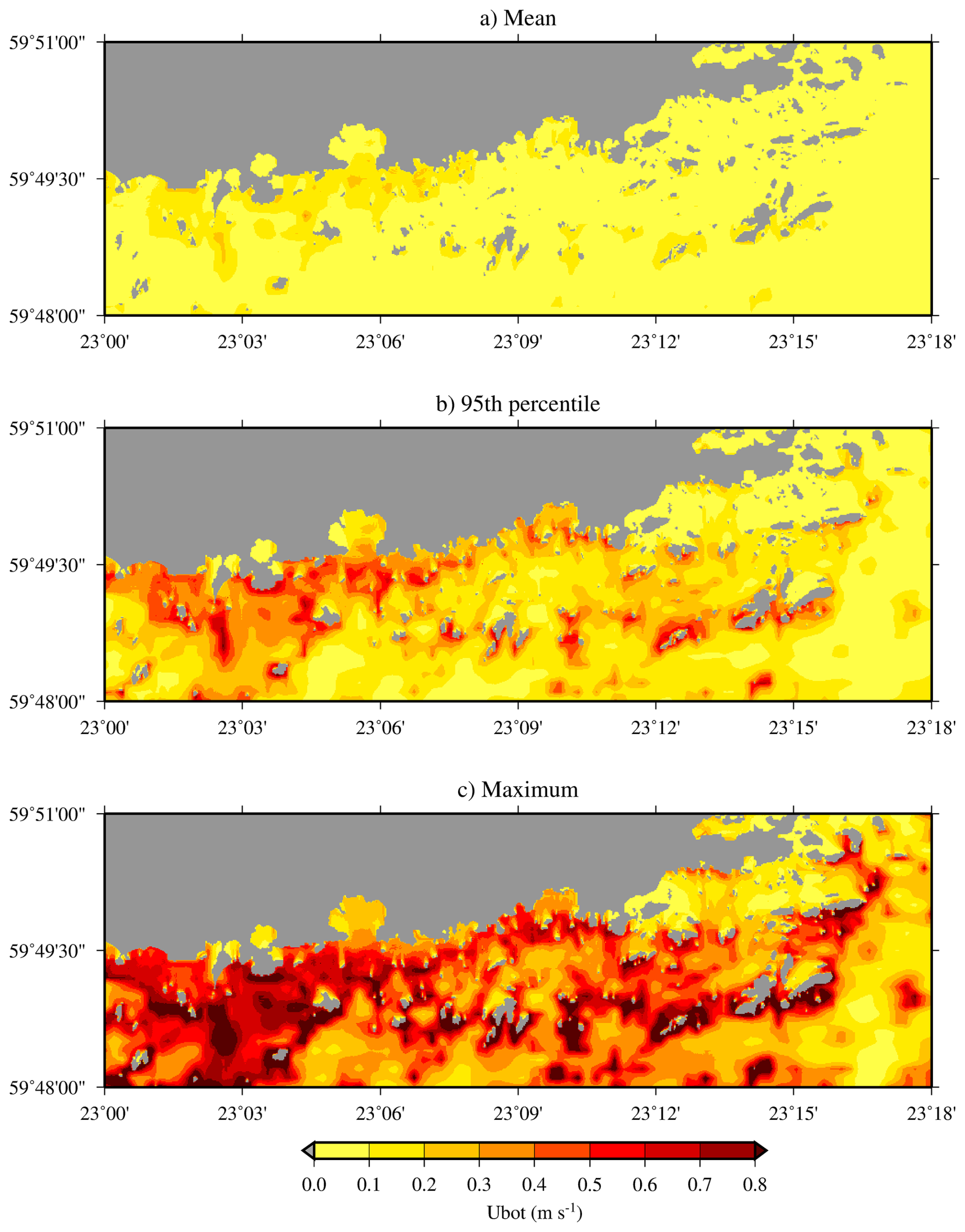
Figure B1 Near-bottom velocities (U_bot) as modelled by the SWAN model.

Appendix C: Validation of wave model performance at outer and inner wave buoys

Figures C1 and C2 presents the validation of the SWAN wave model against in situ measurements from the outer and inner wave buoys.

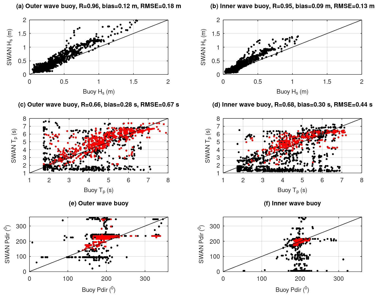
Figure C1 Model-observation scatterplots for significant wave height (H_s), peak wave period (T_p) and mean wave direction at the outer and inner buoys. The locations of the buoys are indicated in Fig. 2. Black dots: all data, red dots: cases when H_s>0.3 m. The statistics for H_s (upper panels) are calculated from the full data set, and the statistics for T_p (middle panels) from the data set with H_s>0.3 m.

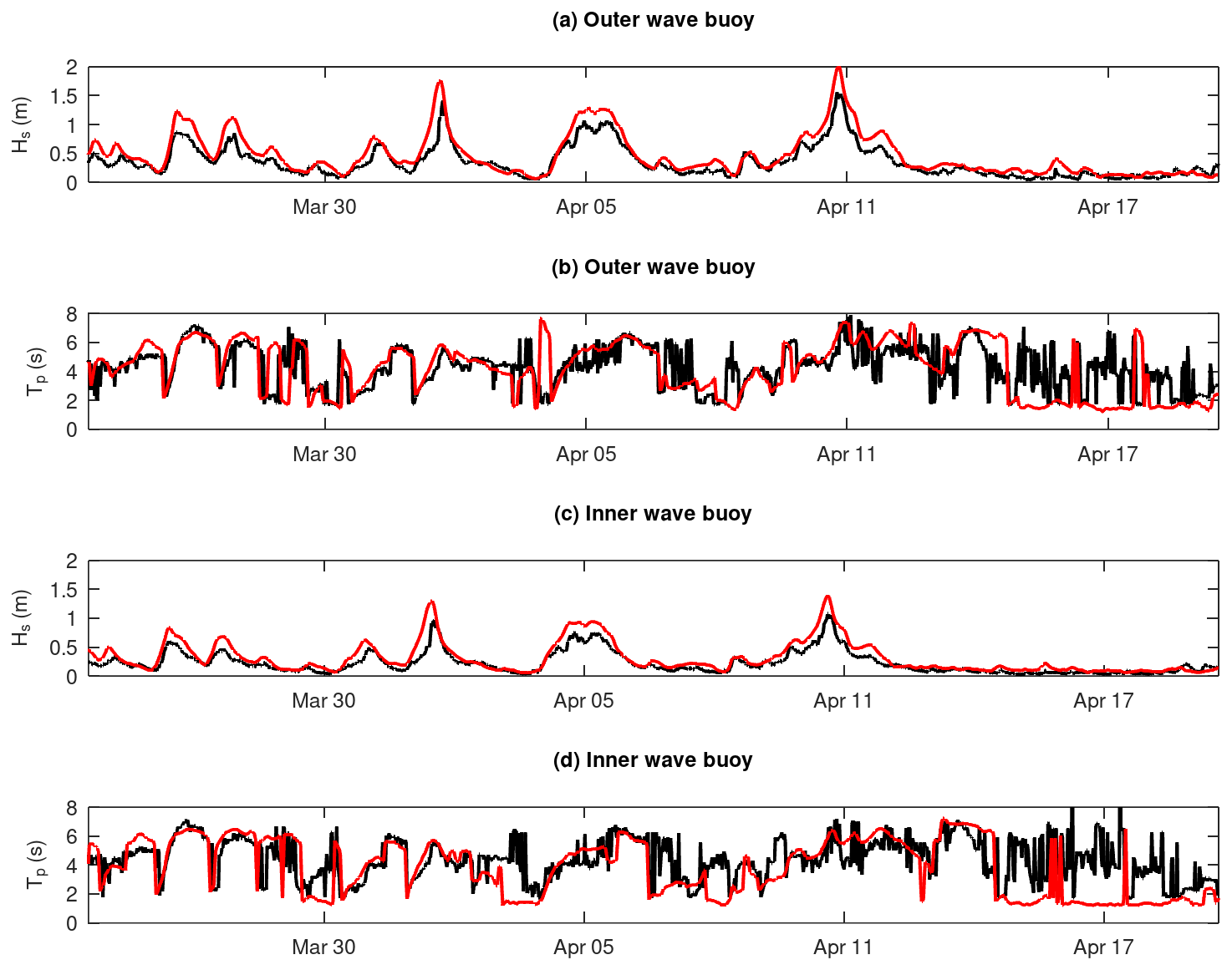
Figure C2 Time series of significant wave height (H_s) and peak wave period (T_p) from buoy observations (black lines) and SWAN model output (red lines) at the outer and inner buoys.