Along-channel variability of Total Exchange Flow in a narrow, well-mixed estuary: influence of the M4 tide

This study provides preliminary estimates of Total Exchange Flow (TEF) along the Guadalquivir River Estuary (Spain) at different cross-sections during low river flows. The analysis combines 3 years of observations from a real-time monitoring network with an analytical exchange flow scenario featuring a sectionally-homogeneous M2+M4 oscillating tidal flow and salinity. Exchange profiles and volume and salinity transports sorted by salinity classes are computed. The results indicate that bulk along-channel TEF estimates decrease upstream.

The largest net incoming water volume transport, on the order of 300 m³ s⁻¹, is attained at the lower part of the estuary, near where the largest salinity gradient is observed. This value is about 12-fold the normal river flow from the head dam at Alcalá del Río. Knudsen bulk quantities are consistent with the weakly-stratified character of the Guadalquivir estuary, whose mixing completeness is larger than 67 % at all cross-sections. The covariance between M2 salinity and current seems to play a more important role in exchange flow in the Guadalquivir estuary than the effects due to tidal asymmetry.

Overall, the inclusion of the M4 improves TEF estimates in ∼ 10 % in the Guadalquivir estuary. A sensitivity analysis shows that in other estuaries and semi-enclosed basins the effects of the M4 could be even larger. The inclusion of the M4 constituent changes the exchange flow profile by salinity class, modifying the range of salinities of both outflows and inflows.

1 Introduction

Knudsen (1900) proposed the simplest, yet insightful quantification of the steady-state exchange flow by considering the volume and salt budget in estuaries (see Knudsen work's translation by Burchard et al., 2018a). The exchange flow is defined here as the tidally-averaged, along-channel net water volume transport inflow (Q_in) and outflow (Q_out) through an estuarine cross-section (Geyer and MacCready, 2014). Assuming that the river discharge Q_r enters the estuary at zero salinity, the long-term averaged volume and salt budgets in an estuary bounded by a fixed transect have been formulated by Knudsen (1900) as

$$\begin{array}{}\text{(1)}& Q_{\text{in}}+Q_{\text{out}}+Q_{\mathrm{r}}=\mathrm{0},Q_{\text{in}}{s}_{\text{in}}+Q_{\text{out}}{s}_{\text{out}}=\mathrm{0},\end{array}$$

where s_in and s_out are the characteristic inflow and outflow salinities, respectively, at the location of the bounding transect. The classical Knudsen relations,

$$\begin{array}{}\text{(2)}& Q_{\text{in}}={\displaystyle \frac{s_{\text{out}}}{s_{\text{in}}-s_{\text{out}}}}{Q}_{\mathrm{r}},Q_{\text{out}}=-{\displaystyle \frac{s_{\text{in}}}{s_{\text{out}}-s_{\text{in}}}}{Q}_{\mathrm{r}},\end{array}$$

are directly derived from Eq. (1) and allow calculating the inflowing and outflowing volume transport which are otherwise difficult to estimate. Using the Knudsen relations (Eq. 2), the exchange flow is thus conveniently estimated in terms of simple bulk values (i.e. Knudsen-bulk values or estimates) which condense the complex dynamics of the exchange flows in estuaries. The Knudsen relations implicitly include mixing of the freshwater discharge with the inflowing ocean water of salinity s_in, and the volume-integrated (bulk) mixing M, which is understood as the salinity variance destruction in the estuary, could be quantified as M=s_ins_outQ_r (MacCready et al., 2018).

The Total Exchange Flow (TEF) analysis framework provides one consistent calculation method that allows for computing the exchange flow and its characteristic salinities using salinity (isohaline) coordinates (MacCready, 2011; Burchard et al., 2019). With this, TEF provides for each estuarine transect profiles of transports of volume and salt per salinity class, as function of a salinity coordinate substituting the two-dimensional Eulerian coordinate of the transect, a method that substantially simplifies the representation of the exchange flow. Moreover, the TEF could be mapped back from salinity coordinates to vertical (Eulerian) coordinates. However, as shown by several authors (MacCready, 2011; Sutherland et al., 2011; Burchard et al., 2018a), this Eulerian method strongly underestimates the exchange flow. A parcel of water that is flowing into the estuary across the transect at a certain salinity class and afterwards flowing out at the same salinity class but possibly at a different area of the transect (i.e., without having been mixed), does not contribute to TEF. In contrast to that, such an exchange of water parcels without mixing would contribute to Eulerian exchange flow. This shows that TEF is closely related to salinity mixing in estuaries (see Burchard et al., 2025b, for more details). The TEF analysis framework determines the most representative Knudsen-bulk estimates by finding the correct values of s_in and s_out, namely the Knudsen-consistent salinity values or estimates. Tidally-averaged net volume and mass transport through an estuarine cross-section are thus obtained sorted by salinity classes (transports as a function of salinity class). Among its outstanding features are: TEF estimates include transports due to covariance of current velocity and salinity, thereby generalizing the classical Knudsen relations; and TEF naturally allows quantifying volume-integrated mixing, which in turn controls the inflow and outflow transport of water and salinity.

Burchard et al. (2019) proposed a simple, sectionally-homogeneous analytical scenario considering only the M2 constituent to show that TEF can also develop even under tidally-energetic conditions. The oscillating exchange flow scenario required prescribing M2 tidal amplitudes and phases in such a way that a specified runoff was obtained and that the residual salt transport is zero. These authors obtained Knudsen-bulk estimates for inflow and outflow of water and their corresponding salt concentrations from TEF analysis. Lorenz et al. (2019) provided an algorithm which extends the formulation of the dividing salinity method (MacCready et al., 2018). The algorithm allows to overcome numerical issues regarding the practical computation of TEF for a large number of salinity classes, thereby ensuing convergence to the TEF bulk values. These authors used the same simple analytical tidal scenario to test the extended dividing salinity method and its convergence. The goodness of the convergence behavior allows extending the method to exchange flows with more than two layers in the salinity space (see, e.g., Burchard et al., 2025a).

However, the influence of tidal asymmetry on TEF remains unexplored. The non-linear generation of the overtide M4 from the primary tidal constituent M2 is known to create ebb-flood asymmetry in water levels and currents (e.g. Speer and Aubrey, 1985; Parker, 1991; Friedrichs and Aubrey, 1994) and affects the transport of solutes and particulate matter (e.g. de Swart and Zimmerman, 2009; Burchard et al., 2018b). Consequently, it is expected to have an impact on TEF. In this study, the M2 oscillating exchange flow scenario devised by Burchard et al. (2019) is extended to include the contribution of the M4 tidal constituent, thereby requiring the prescription of both M2 and M4 amplitudes and phases both in current and salinity. The extended approach is applied to the Guadalquivir estuary, which is a tidally-energetic estuary, to estimate TEF at various cross-sections. While previous TEF research has focused predominantly on highly- or partially-stratified semi-enclosed basins, the tidally-energetic part of the estuarine parameter space has been overlooked. Furthermore, no TEF estimates currently exist for the Guadalquivir estuary. Quantifying TEF from observations and unraveling the role of the M4 constituent in the Guadalquivir estuary is essential for understanding its direct implications for water quality, residence times, and primary productivity (e.g. Díez-Minguito and de Swart, 2020; Castillo et al., 2025). A sensitivity analysis of TEF to the inclusion of the M4 to the tidal current and salinity equations is carried out in this study as well.

To address the estimates of TEF in the Guadalquivir estuary, high-resolution field data of along-channel currents and salinity at seven cross-sections was the basis for the analysis. Observations were automatically recorded between 2008 and 2011 by a real time monitoring network (Navarro et al., 2011). The Guadalquivir estuary is a flood-dominated, tidally-energetic estuary that features a well-mixed to partially mixed (near the mouth) water column during low river flow conditions (Díez-Minguito et al., 2012, 2013). The analysis combines those observations with the M2+M4 oscillating exchange flow scenario. Exchange profiles and volume and salinity transports sorted by salinity classes were computed. To address the sensitivity analysis of the TEF to the overtide M4, a set of simulations was performed including the M4 contribution to the tidal currents and salinity. The ratio between M4 and M2 current and salinity amplitudes, as well as the difference between M4 current and salinity phases, is varied. Effects in exchange profiles, and thus in volume transports, salinities, and salt transports, are examined.

The study is organized as follows. Section 2 sets the TEF framework and introduces the oscillating exchange flow scenario, including both the M2 and M4 constituents (Sect. 2), and describes the Guadalquivir estuary study area (Sect. 2.3) and the field measurements recorded in it (Sect. 2.4). The TEF estimates are described in the Results and Discussion Sect. 3. The results, along with the sensitivity analysis of the TEF to the overtide M4, and their implications are discussed in the same Section. Main conclusions are drawn in Sect. 4.

2 Formulation and Methodology

2.1 TEF Framework

According to the TEF analysis framework, the time-averaged volume transport per salinity class Q through a given cross-section A with salinity s greater than a given value S is obtained as

$$\begin{array}{}\text{(3)}& Q\left(S\right)=\stackrel{\mathrm{‾}}{\underset{A(s\ge S)}{\int }u\mathrm{d}A},\end{array}$$

where the bar $\stackrel{\mathrm{‾}}{\cdot }$ indicates time-averaging, and u is the along-channel current normal to the cross-section A. Changes in cross-sectional area due to tides are not taken into account.

From Eq. (3) the exchange profile of water transport per salinity class is obtained as

$$\begin{array}{}\text{(4)}& q\left(S\right)=-{\displaystyle \frac{\mathrm{d}Q\left(S\right)}{\mathrm{d}S}},\end{array}$$

which verifies $Q={\int }_{s\ge S}q\left(s\right)\mathrm{d}s$. Separating incoming and outgoing volume transports, it reads

$$\begin{array}{}\text{(5)}& Q_{\text{in}}=\underset{S_{\text{min}}}{\overset{S_{\mathrm{0}}}{\int }}q\mathrm{d}s,Q_{\text{out}}=\underset{S_{\mathrm{0}}}{\overset{S_{\text{max}}}{\int }}q\mathrm{d}s,\end{array}$$

where S₀ is the dividing salinity which separates the inflow and outflow, and S_min and S_max are the minimum and maximum salinities in the cross-section. In general, Eq. (5) assumes the incoming and outgoing flows are arranged in two layers in the salinity space (not necessarily in the vertical coordinates as occurs with the classical estuarine circulation). Lorenz et al. (2019) also generalized the formulation for exchange flows with more than two layers in the salinity space.

Similarly to Eqs. (3) and (4), the time-averaged transport of salt, Q^s, reads

$$\begin{array}{}\text{(6)}& Q^{\mathrm{s}}\left(S\right)=\stackrel{\mathrm{‾}}{\underset{A(s\ge S)}{\int }su\mathrm{d}A},\end{array}$$

where $Q^{\mathrm{s}}={\int }_{s\ge S}{q}^{\mathrm{s}}\left(s\right)\mathrm{d}s$ and

$$\begin{array}{}\text{(7)}& Q_{\text{in}}^{\mathrm{s}}=\underset{S_{\text{min}}}{\overset{S_{\mathrm{0}}}{\int }}{q}^{\mathrm{s}}\mathrm{d}s,Q_{\text{out}}^{\mathrm{s}}=\underset{S_{\mathrm{0}}}{\overset{S_{\text{max}}}{\int }}{q}^{\mathrm{s}}\mathrm{d}s.\end{array}$$

Based on quantities defined in Eqs. (5) and (7), Kundsen-consistent salt concentrations for in- and outflows at a cross-section are

$$\begin{array}{}\text{(8)}& s_{\text{in}}={\displaystyle \frac{Q_{\text{in}}^{\mathrm{s}}}{Q_{\text{in}}}},s_{\text{out}}={\displaystyle \frac{Q_{\text{out}}^{\mathrm{s}}}{Q_{\text{out}}}}.\end{array}$$

From Eq. (8) and the bulk mixing M≈s_ins_outQ_r, considering the maximum possible mixing, i.e. $M_{\text{max}}=s_{\text{in}}^{\mathrm{2}}{Q}_{\mathrm{r}}$, the mixing completeness is defined as the ratio between both (MacCready et al., 2018; Burchard et al., 2019)

$$\begin{array}{}\text{(9)}& \mathrm{MC}=M/M_{\text{max}}=s_{\text{out}}/s_{\text{in}}.\end{array}$$

2.2 Oscillating and Well-Mixed Tidal Flow

Tidal current and salinity are assumed a superposition of the main semidiurnal constituent M2 and their most energetic overtide M4 as

$$\begin{array}{}\text{(10a)}& {\displaystyle }\begin{array}{rl}u(x,t)=u_{\mathrm{r}}\left(x\right)& +u_{\mathrm{a}}\left(x\right)\cos \left({\mathit{\omega }}_{\mathrm{M}\mathrm{2}}t\right)\\ & +u_{\mathrm{b}}\left(x\right)\cos ({\mathit{\omega }}_{\mathrm{M}\mathrm{4}}t+{\mathit{\phi }}_{\mathrm{b}}(x\left)\right)\end{array}\text{(10b)}& {\displaystyle }\begin{array}{rl}s(x,t)=s_{\mathrm{r}}\left(x\right)& +s_{\mathrm{a}}\left(x\right)\cos ({\mathit{\omega }}_{\mathrm{M}\mathrm{2}}t+{\mathit{\psi }}_{\mathrm{a}}(x\left)\right)\\ & +s_{\mathrm{b}}\left(x\right)\cos ({\mathit{\omega }}_{\mathrm{M}\mathrm{4}}t+{\mathit{\psi }}_{\mathrm{b}}(x\left)\right)\end{array}\end{array}$$

with x indicating the along-channel location of the cross-section, u_r the residual current induced by the river flow, s_r the residual or tidally-averaged salinity, u_a and u_b the current M2 and M4 amplitudes, φ_b the current M4 phase relative to that of the M2, s_a and s_b the salinity M2 and M4 amplitudes, and ψ_a and ψ_b the salinity M2 and M4 tidal phases relative to the current M2 phase. Residuals, amplitudes and phases are obtained (and prescribed) from field measurements (described below). Tidal periods are $T_{\mathrm{M}\mathrm{2}}=\mathrm{2}\mathit{\pi }/{\mathit{\omega }}_{\mathrm{M}\mathrm{4}}$ = 12.42 h and $T_{\mathrm{M}\mathrm{4}}=\mathrm{2}\mathit{\pi }/{\mathit{\omega }}_{\mathrm{M}\mathrm{4}}$ = 6.21 h.

The tidally-averaged (residual) salinity flux $\stackrel{\mathrm{‾}}{u\cdot s}$ through a given cross-section at x is obtained from Eqs. (10a) and (10b) as

$$\begin{array}{}\text{(11)}& \stackrel{\mathrm{‾}}{u\cdot s}=u_{\mathrm{r}}{s}_{\mathrm{r}}+{\displaystyle \frac{u_{\mathrm{a}}{s}_{\mathrm{a}}}{\mathrm{2}}}\cos \left({\mathit{\psi }}_{\mathrm{a}}\right)+{\displaystyle \frac{u_{\mathrm{b}}{s}_{\mathrm{b}}}{\mathrm{2}}}\cos ({\mathit{\phi }}_{\mathrm{b}}-{\mathit{\psi }}_{\mathrm{b}}).\end{array}$$

Zero residual salinity flux, i.e. $\stackrel{\mathrm{‾}}{u\cdot s}=\mathrm{0}$, implies

$$\begin{array}{}\text{(12)}& \cos \left({\mathit{\psi }}_{\mathrm{a}}\right)=-\mathrm{2}{\displaystyle \frac{u_{\mathrm{r}}{s}_{\mathrm{r}}}{u_{\mathrm{a}}{s}_{\mathrm{a}}}}-{\displaystyle \frac{u_{\mathrm{b}}{s}_{\mathrm{b}}}{u_{\mathrm{a}}{s}_{\mathrm{a}}}}\cos ({\mathit{\phi }}_{\mathrm{b}}-{\mathit{\psi }}_{\mathrm{b}}).\end{array}$$

This zero flux condition reduces the degrees of freedom of the problem to eight, to be determined from observations: u_r, s_r, u_a, s_a, u_b, s_b, φ_b and ψ_b. Considering the M2 tide only in Eqs. (10a) and (10b), as in Burchard et al. (2019); Lorenz et al. (2019), the condition of zero residual salinity transport would reduce to $\cos \left({\mathit{\psi }}_{\mathrm{a}}\right)=-\mathrm{2}\left(u_{\mathrm{r}}{s}_{\mathrm{r}}\right)/\left(u_{\mathrm{a}}{s}_{\mathrm{a}}\right)$.

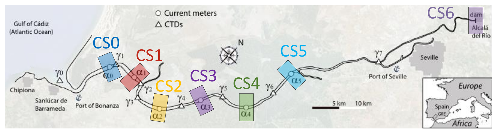
Figure 1 Map of study area. Data in this work is obtained from current-meter profilers, ADCPs (circles, α_i), and environmental quality probes or CTDs (triangles, γ_i). Cross-sections CS_i (Fig. 1), with $i=\mathrm{0},\mathrm{\dots },\mathrm{5}$ are defined by the location of the current meters α_i. Salinity tidal data are linearly interpolated at α_i locations.

2.3 Study Area

The Guadalquivir River Estuary is a coastal-plain estuary located in the south-western part of the Iberian Peninsula. The Guadalquivir estuary comprises the last 110 km of the Guadalquivir river, from head dam at the town of Alcalá del Río to Sanlúcar de Barrameda, where its waters flow into the Gulf of Cádiz in the Atlantic Ocean (Fig. 1). The estuary is convergent with tidally-averaged cross-sections approximately decreasing exponentially from the mouth to the landward end according to

$$\begin{array}{}\text{(13)}& A\left(x\right)=A_{\mathrm{0}}\exp (-x/a_{\mathrm{0}}),\end{array}$$

with A₀ = 5800₉₀₀ m² and a₀ = 60₅ km, where the subscript indicates the 95 % confidence interval in the last significant figure. Its mean depth in the thalweg, h≈ 7 m, is maintained by periodic dredging of the navigation channel (Sirviente et al., 2023). Tides are mesotidal (vertical tidal range at spring tides ∼ 3.5 m at the mouth) and semidiurnal, M2 being the most significant constituent. The estuary is flood-dominated as evidenced by the tidal phase differences between M2 and its first overtide M4, which accounts for (intra)tidal asymmetry (Díez-Minguito et al., 2012). The tide propagation is dominated by friction and in the upper part by tidal wave reflection at the head dam of Alcalá del Río dam (Díez-Minguito et al., 2012; Muñoz-Lopez et al., 2024).

The climate in most of the Guadalquivir River basin is Mediterranean, characterized by hot, dry summers and mild, rainy winters. The basin is highly altered by human activities, with the discharge regime largely controlled by extensive upstream regulation and long-term land-use changes. Freshwater discharges inputs to the estuary from the Alcalá del Río dam are usually below Q_r = 40 m³ s⁻¹, most often about Q_r∼ 25 m³ s⁻¹. Salinity decreases from the mouth upstream due to freshwater input. The mesotidal conditions along with the relatively low values of Q_r make the estuary tidally-energetic and well-mixed (partially-mixed near the mouth) in terms of salinity during low river flows. This is confirmed by the low values of the estuarine Richardson number (Ri_E < 0.08) and the potential energy anomaly (Cobos et al., 2020). Díez-Minguito et al. (2013) determined from an observational analysis that time correlation between tidal flow and salinity controls a substantial part of the salt transport. Modeling results by Biemond et al. (2024) showed that the salt transport due to the density-driven flow interacts with that of the current-salinity correlation and that both transports are equally important in the Guadalquivir estuary. Under low river flow conditions, most of the observed suspended matter in the Guadalquivir estuary is due to the resuspension by tidal currents (Díez-Minguito et al., 2014; Díez-Minguito and de Swart, 2020). The transport due to the M2 and M4 covariance of current velocity and suspended sediment explains the setting of Estuarine Turbidity Maxima in the Guadalquivir estuary (Caballero et al., 2014; Díez-Minguito et al., 2014).

2.4 Data Collection

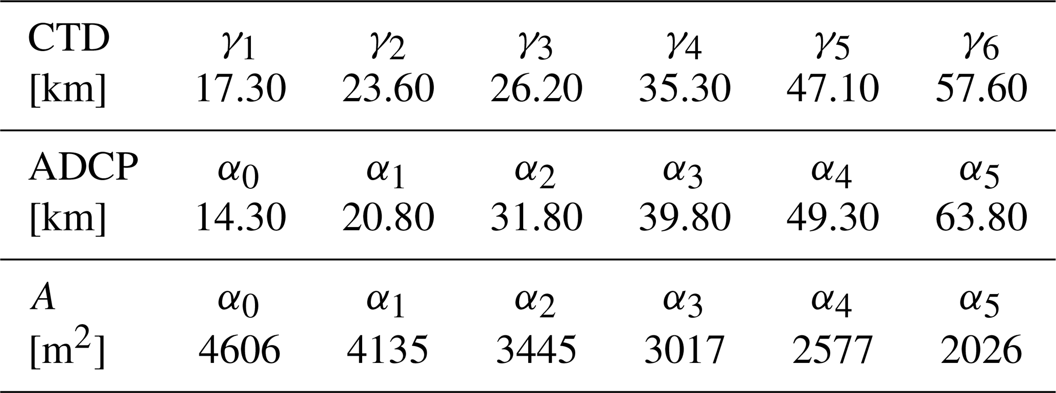
Salinity and current data were recorded between 2008 and 2011 by a real time monitoring network, which was described in detail by Navarro et al. (2011) and depicted in Fig. 1. Here only a brief description of the equipment is provided. Instrumentation was installed as close as possible to the navigation channel. Salinity data was recorded every 30 min in eight Conductivity-Temperature-Depth (CTD, denoted by γ_i in Fig. 1) probes. The origin of the along-channel coordinate x was set at γ₀, installed at the mouth of the estuary, and chosen chosen positive upstream. Table 1 shows the locations of the CTDs used in this study. Along-channel current data was obtained from six Acoustic Doppler Current Profilers (ADCPs) (α_i in Fig. 1), providing one data set every 15 min. Table 1 shows the kilometer points and geographic coordinates where the ADCPs were located in the Guadalquivir estuary.

Table 1 Locations where the CTDs (γ_i) and ADCPs (α_i) were located, with respect to the estuary mouth, and tidally-averaged cross-sections computed using Eq. (13) at the ADCP locations.

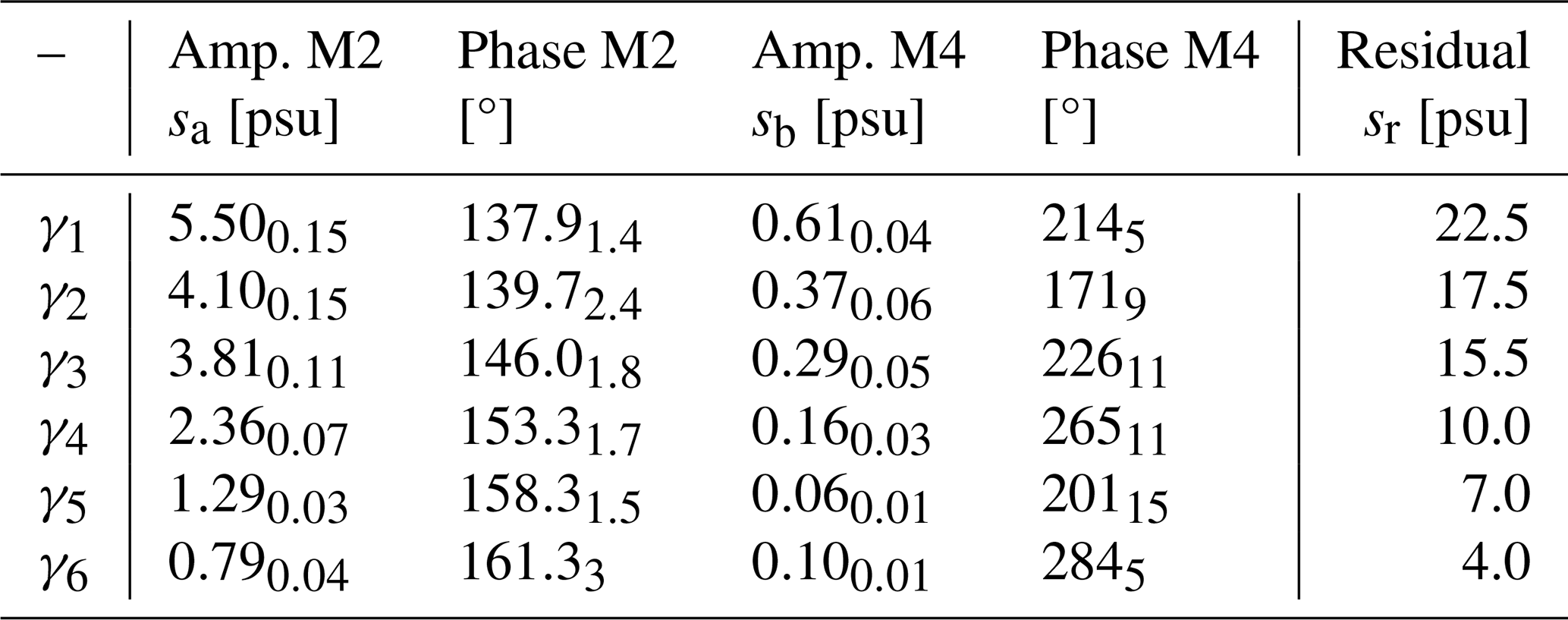
Standard harmonic analysis was performed on the along-channel current and salinity time series using T_TIDE (Pawlowicz et al., 2002). Results are shown in Tables 2 and  3. The time span for the harmonic analysis was 5 June 2008 through 5 December 2008. This time span was chosen according to the following three criteria. The interval must be larger than 28 d to separate the M2 from other semidiurnal constituents and to assure a zero residual net salt flux. And, finally, the chosen interval is that one with the fewer and smaller exceedances over 40 m³ s⁻¹ to assure that the data analysis corresponds with low river flow conditions.

Table 2 Harmonic analysis of the along-channel horizontal tide time series. Amplitudes are in cm s⁻¹ and phases in ° Greenwich. Errors (subscripts) corresponds to the 95 % confidence interval. Subtracting the current M2 phase to the current M4 phase, φ_b is obtained as the M4 phase relative to that of the M2, as defined in Eqs. (10a) and (10b).

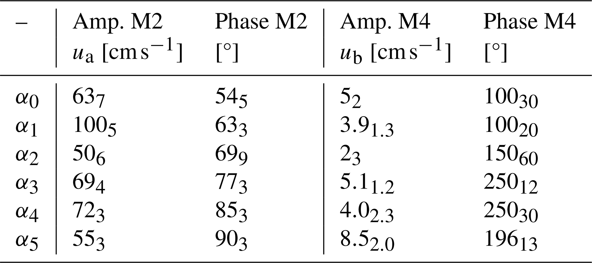
Table 3 Harmonic analysis of the salinity time series. Residual values and amplitudes are in psu and phases in ° Greenwich. Errors (subscripts) corresponds to the 95 % confidence interval. Subtracting the current M2 phase to the salinity M2 and M4 phases, ψ_a and ψ_b are obtained as the salinity M2 and M4 tidal phases relative to the current M2 phase, respectively, as defined in Eqs. (10a) and (10b).

Daily discharge data records at Alcalá del Río were provided by the Regional Water Management Agency (Red de seguimiento de la Confederación Hidrográfica del Guadalquivir, MAPAMA, station code 5072).

3 Results and Discussion

3.1 Volume Transports, Exchange Profiles and Bulk Quantities

Volume transports and exchange profiles sorted by salinity classes are computed numerically using the analytical time series from Eqs. (3) and (4), respectively. They are computed at different cross-sections along the Guadalquivir estuary indicated in Table 1 (and Fig. 1). Tidal currents and salinity are obtained from Eqs. (10a) and (10b), which include both the M2 and M4 constituents.

Values of u_r, s_r, u_a, s_a, u_b, s_b, φ_b and ψ_b (Eqs. 3 and 4) at each cross-section in Fig. 1 are thus needed. They are obtained from Tables 2 and 3. From Eq. (12), ψ_a is also computed from the other eight parameters at each cross-section. Differences between observed values of ψ_b (Table 3) and those determined from Eq. (12) imposing zero residual salt flux are smaller than 12° at all cross-sections, i.e., $\mathit{\{}\mathrm{5.45}\mathit{°},\mathrm{11.20}\mathit{°},\mathrm{1.70}\mathit{°},\mathrm{5.54}\mathit{°},\mathrm{7.80}\mathit{°},\mathrm{2.16}\mathit{°}\mathit{\}}$. Therefore, at the analysis scale, the estuary can be reasonably considered close to equilibrium conditions (zero residual salt flux).

Figure 2 shows the isohaline volume transport (solid lines) and the exchange profile (dotted lines), which are computed numerically using analytical time series according to Eqs. (3) and (4), respectively, as a function of the salinity at cross-sections CS_i. Overall, as the tide propagates upstream, i.e., towards estuarine parts of lower salinity and current, the maximum values of Q(S) become smaller. The largest volume transports Q(S) are observed at the CS₁ and CS₀ cross-sections, which are in the lower part of the estuary where the tidal currents are larger. The exchange profile q(S) per salinity class is structured in two layers at all locations, thereby showing a incoming transport of water per salinity class (q_in) at higher salinity and an outgoing transport at lower salinity (q_out). It is evident from Fig. 2 that incoming and outgoing transport vary more by salinity class in locations near the estuary mouth.

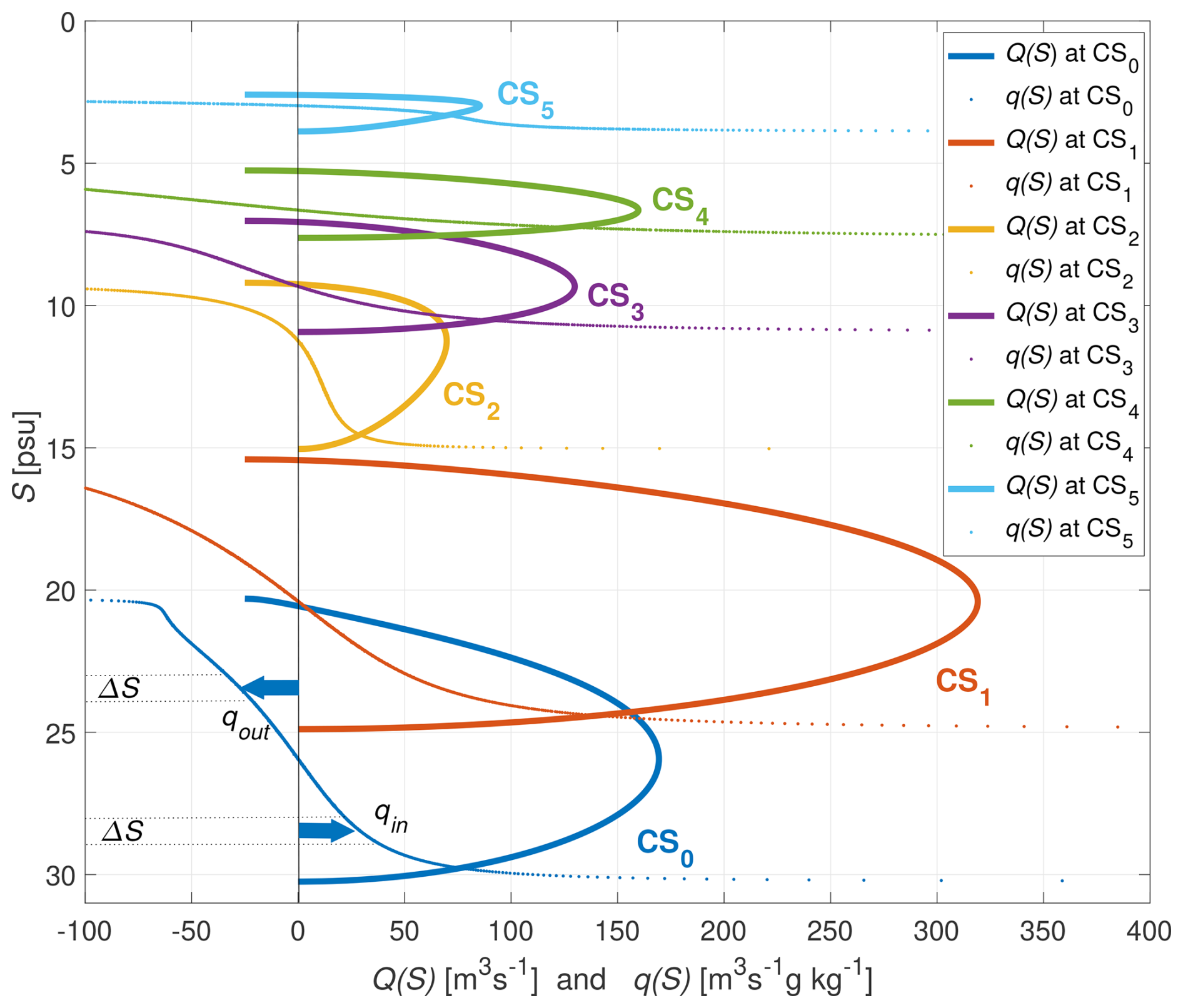
Figure 2 Volume transports Q(S) (solid curves) and exchange profiles (dotted curves) q(S) sorted by salinity classes are computed at cross-sections CS_i. Note the inversion of the vertical axis.

Figure 3 shows the Knudsen-bulk estimates along the main channel determined from the TEF analysis, Q_in and Q_out, determined integrating q_in and q_out (Eq. 5), i.e. positive and negative transports, respectively. The results indicate that bulk along-channel exchange flow tends to decrease upstream, as expected. Incoming and outgoing water volume transports estimated here in the lower part of the estuary are about 10 % larger than volume transports inferred from the tidally-averaged horizontal current profiles shown by Reyes-Merlo et al. (2013), who considered the density-driven flow only using an Eulerian approach at CS₀ and CS₁. This estimate difference from different approaches will be further discussed in Sect. 3.4. At the landward boundary at the head dam (CS₆), the outgoing volume transport coincides with the freshwater discharge Q_r = −25 m³ s⁻¹. Negligible values are obtained in the upper part of the estuary near the head dam. In the middle part of the estuary, incoming TEF bulk volume values below 150 m³ s⁻¹ are obtained. The largest net incoming water volume transport, viz. Q_in≈ 300 m³ s⁻¹, is attained at the lower part of the estuary at CS₁. The outgoing bulk value at CS₁ is about 12-fold the normal river flow from the head dam at Alcalá del Río.

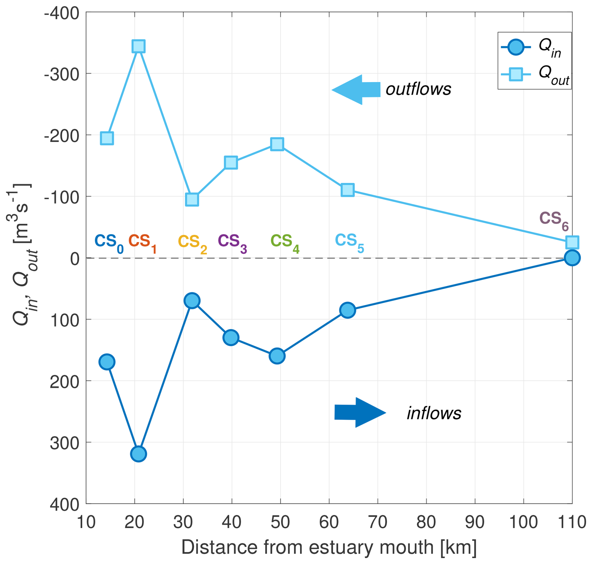
Figure 3 Outgoing Q_out (light blue curve, squares) and incoming Q_in (dark blue curve, circles) volume transports at each cross-section CS_i.

It is evident from the TEF results shown in Fig. 3 that the exchange flow does not decrease continuously from the estuary mouth to the head. The along-channel variability of the bulk estimates (from Eq. 7) are mainly due to changes in the along-channel currents and distribution of salinity. Cross-section CS₁ is the closest to where the largest (averaged) along-channel salinity gradient (Díez-Minguito et al., 2013) and where the largest tidal currents are observed (Table 2). The relative exchange flow mininum at cross-section CS₂ is caused by a significant decrease of the M2 tidal current amplitude (Table 2). A plausible source of variability could be due lateral variations in the along-channel current over the cross-section. Although instrumentation was installed as close as possible to the main channel of the estuary, the particular mooring location of each current meter may also affect tidal current amplitudes and, thus, TEF estimates. The exchange flow minimum at cross-section CS₂ suggests that further upstream outflows are convergent and inflows are divergent, which can only be explained by a partial recirculation of the outflow towards the estuary head. Directly downstream of the minimum, outflow is divergent and inflow is convergent such that parts of the inflow is deflected back towards the mouth of the estuary. This mechanism has been described by Cokelet and Stewart (1985) as the efflux/reflux theory. In practice, this would imply longer residence times for conservative pollutants than in the absence of recirculation.

It should be noted that exchange flow in a well-mixed estuary does not mean that there is a distinct upstream flow of salty water near the bottom and a downstream flow of brackish water near the surface, even though the exchange profiles in salinity coordinates q(S) are structured in two layers (as in Fig. 2). The exchange flow following the Knudsen (1900) theory is formulated in salinity coordinates and means that the outflow Q_out occurs at lower salinities than the inflow Q_in. During flood a water parcel with a specific salinity passes through a transect, leaving an upstream flux contribution at a certain salinity class. Upstream of the transect, this water parcel exchanges salinity with other water parcels, such that during ebb it passes the transect at a different salinity, leaving a downstream contribution at this different salinity. Statistically, the flood flux happens at a higher salinity than the ebb flux, due to the lower salinities upstream, caused by the freshwater discharge from the upstream dam. This is why the fully cross-sectionally mixed idealized estuarine situation described in Eqs. (10a) and (10b) still results in an estuarine exchange flow, when formulated in salinity coordinates. Given that the Guadalquivir estuary is well-mixed during low river discharge, except for its partially-mixed lower part near the mouth, a vertically-structured exchange flow with persistent deep-water inflow and surface outflow might only develop in that lower region.

Figure 4 shows the along-channel Knudsen-consistent salt concentration estimates within inflows and outflows at each cross-section. Both curves resemble the (averaged) salinity along-channel distribution of salinity. The representative TEF bulk salinity values for the incoming transport are larger than those for the outgoing transport. Differences increase towards the estuary mouth from the head dam, where $s_{\text{in}}=s_{\text{out}}=\mathrm{0}$. At CS₀, which is the cross-section nearest to the mouth, the representative TEF bulk salinity value for inflows is 28 psu, whereas that for outflows at the same location is about 21 psu. Where the largest net incoming water volume transport occurs (CS₁) these values are 16 and 24 psu, respectively.

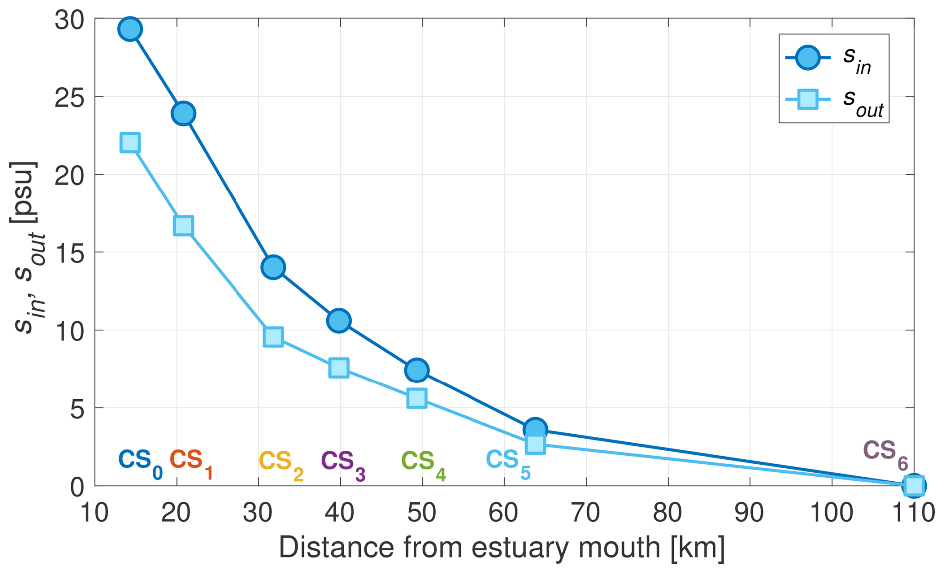
Figure 4 Knudsen-consistent salinities for in- (dark blue curve, circles) and outflows (light blue curve, squares) at cross-sections along the estuary.

3.2 Mixing Completeness

The small relative differences between representative TEF bulk salinity values for inflows and outflows, i.e. $\mathrm{1}-s_{\text{out}}/s_{\text{in}}$ (Fig. 4), ensue from the high rates of mixing in the Guadalquivir estuary. The analysis of salt transport indicates that the mixing completeness, estimated from Eq. (9) (in %), is larger than 67 % at all cross-sections (Fig. 5), thereby evidencing the poorly-stratified character of the Guadalquivir estuary during low river flows. The mixing completeness attains at the cross-section nearest to the mouth of the estuary. The net TEF exchange of variance upstream, at the tidal river part, is negligible due to vanishing salinities, such that the mixing is complete (100 %). Mixing completeness values in the lower and middle part of the Guadalquivir estuary, which are between 70 % and 75 %, are similar to the 75 % estimated near the mouth of the Elbe during low discharge conditions (Reese et al., 2024). The estimated values in the Guadalquivir are not far from those obtained in and idealized convergent V-shaped model estuary, viz. 64 % (MacCready et al., 2018), which seems reasonable as the Guadalquivir estuary is a highly channelized estuary. While the mixing completeness can range between zero and 100 % in estuaries (Burchard et al., 2025b), the Guadalquivir estuary can be rated as of relatively high mixing completeness compared to other estuaries which typically at high discharge or neap-tide conditions are more stratified and therefore of lower mixing completeness (below 50 %).

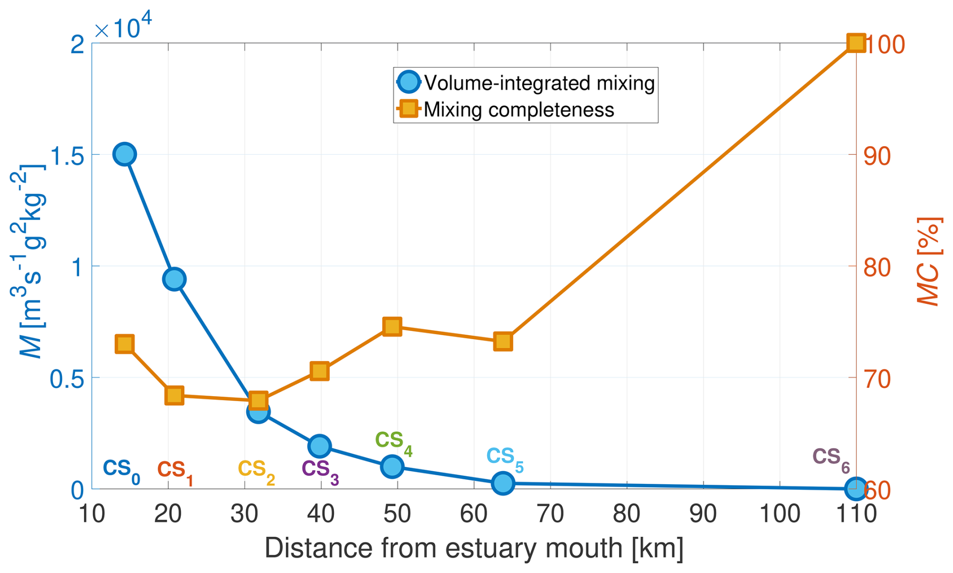
Figure 5 Volume-integrated mixing (left y-axis; dark blue curve, circles) and mixing completeness (right y-axis; dark yellow curve, squares).

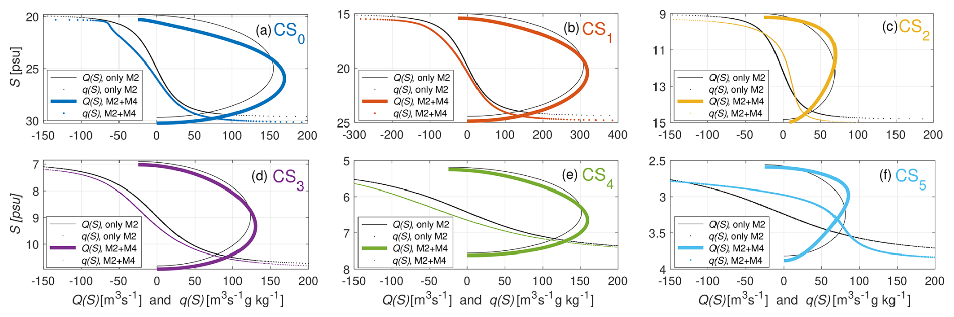
Figure 6 Volume transports Q(S) (solid curves) and exchange profiles (dotted curves) q(S) sorted by salinity classes are computed at cross-sections CS_i considering the superposition of the M2 and M4 constituents (colored curves) and the M2 only, without the M4 contribution (black curves).

3.3 Influence of M4 in Total Exchange Flow

3.3.1 Guadalquivir Estuary

The inclusion of the M4 tidal constituent in the analysis, with regards to the original M2(-only) oscillatory exchange flow analysis by Burchard et al. (2019); Lorenz et al. (2019), produces noticeable effects in both the volume transports Q(S) and exchange profiles q(S). Figure 6 shows results of Q and q per salinity class at cross-sections CS_i for the extended analytical scenario, which includes the M4 and M2 contribution (colored curves), and that with the M2 constituent only (black curves). Colored curves are in fact the same as in Fig. 2. Differences in magnitude between both are evident at all cross-sections, but they are somehow more acute at CS₀ and CS₅. The M4 inclusion does not change the two-layered feature of the exchange profile in salinity coordinates. However, it changes the the range of salinities of each layer in the salinity space. The M4 contribution, which is known to account for the tidal asymmetry, increases the range of salinities of the seaward flow at all cross-sections, except at CS₂ and CS₅ where the lower inflowing salinity range increases due to the relatively low relative M2-M4 phase difference (ψ_a−2 ψ_b) at these locations (Table 3). The changes at all locations are evidenced in the shift of the maxima of Q(S) towards higher salinities and lower salinities, respectively. At all locations the maxima of the volume transports Q(S) are about 10 % larger when considering the superposition of M2 and M4 constituents.

Table 4 Knudsen-bulk values of outgoing and incoming volume transports (Q_out and Q_in, respectively), knudsen-consistent salinities for out- and inflows (s_out and s_in, respectively), and outgoing and incoming salt transports ($Q_{\text{out}}^{\mathrm{s}}$ and $Q_{\text{in}}^{\mathrm{s}}$, respectively) with and without the M4 contribution, i.e., with the M2 tide only, at each cross-section CS_i.

Estimates of volume transports, salinities, and salt transports (with and without the inclusion of M4) obtained from Q(S) and q(S) in Fig. 6 are shown in Table 4. The largest differences due to the inclusion of the M4 are obtained in the cross-section closest to the mouth (CS₀). At this cross-section, percentage differences in outgoing and incoming volume with and without the M4 contribution (Q_out and Q_in) are ∼ 8 % and ∼ 9 %, respectively, whereas differences in Knudsen-consistent salinities are smaller, viz. ∼ 5 % and ∼ 2 %, respectively. This yields increases in outgoing and incoming salt transports ($Q_{\text{out}}^{\mathrm{s}}$ and $Q_{\text{in}}^{\mathrm{s}}$) ∼ 13 % and ∼ 11 %, respectively. At other cross-sections differences in the bulk estimates for inflow and outflow of water and salt do not exceed 8 %. These percentage values are not particularly large, but non-negligible either. This seems to ensue that the covariance between M2 salinity and current is a mechanism more significant controlling the exchange flow in the Guadalquivir estuary than the tidal asymmetry. Notice that the ratio of the M4 and M2 amplitudes is below 16 % for currents and below 13 % for salinities, being the largest ratios observed at CS₀ and CS₅ (see Tables 2 and 3). These two locations are where differences in volume transport and exchange profiles shown in Fig. 6 are the largest.

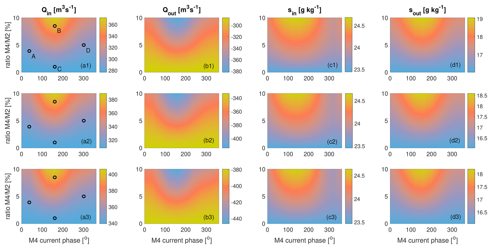
Figure 7 Sensitivity of incoming (panels a1, a2, and a3) and outgoing volume transports (panels b1, b2, and b3) and salinities for inflows (panels c1, c2, and c3) and outflows (panels d1, d2, and d3) to ratio between M4 and M2 current amplitudes ($u_{\mathrm{b}}/u_{\mathrm{a}}$) and to M4 current phase (φ_b). First, second and third row of panels correspond with R = 10 m³ s⁻¹, R = 25 m³ s⁻¹, and R = 40 m³ s⁻¹, respectively. Black circles and capital letters indicate example cases in the parameter space shown in Fig. 8.

With a view to gaining insight into the effects of including M4 and to better interpret the results, these effects are compared with those produced in the TEF by changes in the bathymetry. The outgoing and incoming volume transports with the M4 contribution at each cross-section CS_i are compared with those obtained for the M2 tide only considering bathymetric changes. New incoming and outgoing volume transports are thus estimated when cross-sections according to Eq. (13) are varied, either due to variations in the convergence length a₀ or in the cross-section at the mouth A₀. Reference values a₀ = 60 km and A₀ = 5800 m² are those in Eq. (13). Overall, the increase in the cross-sectional areas, whether due to an increase in the convergence length or in the cross-section at the mouth, enhances the exchange flow. It is found that a change in the convergence length when increased from a₀ = 60 km to 90 km (50 % increase) produces outgoing and incoming volume transports similar to those obtained by including M4 in the section closest to the estuary mouth (CS₀). At the other locations CS_i, the results are reproduced for convergence lengths between 65 and 70 km. Similarly, a sensitivity analysis carried out with the cross-sectional area at the mouth A₀ indicates that a increase from A₀ = 5800 m² to A₀ = 6250 m² (7.75 % increase) produces outgoing and incoming volume transports close to those obtained by including M4 at all cross-sections. Therefore, the increase in TEF due to the inclusion of M4 corresponds to appreciable increases in the cross-sectional areas of the estuary.

3.3.2 Sensitivity Analysis

The effects on TEF due to the inclusion of the M4 in the tidal current and salinity equations depend on the relative differences of amplitudes and phases, thus they could differ in other estuaries or semi-enclosed basins. A sensitivity analysis of TEF to values of current and salinity amplitudes and phases (i.e. those in Eqs. 10a and 10b) and freshwater discharge is thus performed considering values at CS₁ in the Guadalquivir estuary as reference. The analysis is performed only during the low riverflow conditions for R = 10, 25, and 40 m³ s⁻¹. The analysis considers as reference parameters those observed in the cross-section CS₁, which exhibits the largest exchange flow in the Guadalquivir estuary, viz. A = 4135 m², u_a = 1 m s⁻¹, s_r = 19.72 g kg⁻¹, s_a = 4.72 g kg⁻¹, and ψ_b = 127.11°. The residual current is u_r = −0.0024 m s⁻¹ for R = 10 m³ s⁻¹, u_r = −0.0060 m s⁻¹ for $R=\mathrm{25}{\mathrm{m}}^{\mathrm{3}}{\mathrm{s}}^{-\mathrm{1}}$, and $u_{\mathrm{r}}=-\mathrm{0.0097}\mathrm{m}{\mathrm{s}}^{-\mathrm{1}}$ for R = 40 m³ s⁻¹. The M2 salinity phase ψ_a is determined from the zero residual salinity flux condition (Eq. 12). The ratio between M4 and M2 current amplitudes, $u_{\mathrm{b}}/u_{\mathrm{a}}$, is varied from 0 % to 15 %, according to observations in a number of estuaries. The ratio of the M4 and M2 tidal water level amplitudes rarely exceeds 0.15 (Friedrichs and Aubrey, 1988), although higher ratios are usually observed in tidal creeks and tidal flats. Ratios of M4 and M2 tidal current amplitudes in the Guadalquivir estuary range from 0.04 to 0.15 (Table 2). Similar ranges were found by Blanton et al. (2002) in their study on the tidal current asymmetry in the Satilla River estuary. The ratio between M4 and M2 salinity amplitudes, $s_{\mathrm{b}}/s_{\mathrm{a}}$, consistently varies along with the currents from 0 to 0.9059. Current and salinity M4 and M2 amplitudes are chosen not to be independent to match observations in CS₁ when u_b = 0.039 m s⁻¹, s_b = 0.4767 g kg⁻¹ (Tables 2 and  3), and also when u_b=0, s_b=0 (which corresponds with the only M2 case). The difference between M4 current and salinity phases, φ_b−ψ_b, is varied from 0 and 360°.

The inclusion of M4 term in the tidal equations significantly influences bulk quantities of the exchange with regards to the M2 only reference case. The results of this analysis yield differences in volume transports, salinities, and salt transports. Figure 7 shows patterns of incoming (Q_in, Fig. 7 panels a) and outgoing volume transports (Q_out, Fig. 7 panels b) and their respective consistent salinities s_in (Fig. 7 panels c) and s_out (Fig. 7 panels d) in the explored parameter space for R = 10 m³ s⁻¹ (upper row), R = 25 m³ s⁻¹ (middle row), and R = 40 m³ s⁻¹ (lower row). Values for the only M2 reference case correspond with the ratio of M4 and M2 current amplitude $u_{\mathrm{b}}/u_{\mathrm{a}}=\mathrm{0}$. Overall, for R = 10 m³ s⁻¹ (upper panels in Fig. 7), the higher the ratio of M4 and M2 current amplitudes ($u_{\mathrm{b}}/u_{\mathrm{a}}$) and the closer to ∼ 160° the M4 current phase (φ_b) is, the higher the influence in Q_in (Fig. 7a1), Q_out (Fig. 7b1), s_in (Fig. 7c1), and s_out (Fig. 7d1). Differences in Q_in and Q_out between cases including M4 and the case with only M2 can be as much as ± 94 m³ s⁻¹ when the ratio of amplitudes is $u_{\mathrm{b}}/u_{\mathrm{a}}\approx$ 0.10, thereby being Q_in≈ 371 m³ s⁻¹ (panel a1) and Q_out≈ −381 m³ s⁻¹ (Fig. 7b1). Salinity for inflows increases due to the inclusion of the M4 up to s_in = 24.7 psu (+1.2 psu, Fig. 7c1), whereas for outflows increases up to s_out = 19.0 psu (+3.0 psu, Fig. 7d1).

Patterns of the same variables for R = 25 m³ s⁻¹ and R = 40 m³ s⁻¹ are shown in the second and third rows of panels, respectively. The highest bulk values in Q_in (Fig. 7a2 and a3, respectively), Q_out (Fig. 7b2 and b3, respectively), s_in (Fig. 7c2 and c3, respectively), and s_in (Fig. 7d2 and d3, respectively) also occur for large M4 vs. M2 current amplitude ratios and M4 current phase values φ_b≈ 160°. Results also indicate that the higher the freshwater discharge, the higher the exchange. For R = 25 m³ s⁻¹, the highest incoming volume transport bulk value is Q_in≈ 388.90 m³ s⁻¹ (Fig. 7a2) and the lowest outgoing volume attained is Q_out≈ −413.90 m³ s⁻¹ (Fig. 7b2). These values differ about 80 m³ s⁻¹ from what is observed in CS₁ in the Guadalquivir estuary, i.e. for R = 25 m³ s⁻¹, Q_in = 308.2 m³ s⁻¹, Q_out = −333.2 m³ s⁻¹ (same parameters as Case A, and also in Table 4). For R = 40 m³ s⁻¹, the highest incoming and outgoing transports (Q_in≈ 406.25 m³ s⁻¹ (Fig. 7a3) and Q_out≈ −446.25 m³ s⁻¹) (Fig. 7b3) occur at the same phase.

Additionally, in the parameter space explored, as the freshwater discharge increases, both the s_in and s_out values tend to decrease. Regarding differences with respect to the only M2 case, the maxima/minima s_in values slightly decrease/increase with increasing freshwater discharge, i.e. from 23.44–24.68 psu for R = 10 m³ s⁻¹ (Fig. 7c1) to 23.46–24.63 psu for R = 40 m³ s⁻¹ (Fig. 7c3). The maxima/minima s_out values slightly decrease/increase with increasing freshwater discharge, i.e. from 16.02–19.05 psu for R = 10 m³ s⁻¹ (Fig. 7c1) to 16.05–18.19 psu for R = 40 m³ s⁻¹ (Fig. 7c3). Overall, s_in and s_out values are rather insensitive to changes in R within the low river flow range analyzed (R = 10–40 m³ s⁻¹).

Figure 8 shows four example Cases (A, B, C, and D in Fig. 7a1) of modified volume transports Q(S) and exchange profiles q(S) sorted by salinity classes which correspond with four sets of parameters for three different freshwater discharges (Fig. 7a1–a3). Overall, the inclusion of the M4 constituent changes the magnitude of the exchange flow by salinity class, and also the range of incoming and outgoing salinities. The extent of the change depends on the ratio between M4 and M2 current amplitudes ($u_{\mathrm{b}}/u_{\mathrm{a}}$) and to M4 current phase (φ_b). Case A (Fig. 8a) represents the parameters observed at CS₁, incorporating the M4 and M2 tidal constituents for various freshwater discharge rates. This case indicates that the inclusion of M4, relative to the M2-only scenario, increases the range of salinities of outflows in the q(S) profile for all discharge values, viz. R = 10 m³ s⁻¹ (blue curve), R = 25 m³ s⁻¹ (red curve), and R = 40 m³ s⁻¹ (yellow curve). This effect is more pronounced at higher river flows, though the differences are not substantial. Similar patterns are observed in Case D (Fig. 8d), which displays q(S) profiles for comparable M4 vs. M2 ratios to those of Case A but with φ_b≈ 300°. In Case D, it is likewise observed that the inclusion of M4 increases the range of salinities associated to outflows (upper layer of the q(S) profile) compared to the M2-only for the three discharge values simulated, although, again, without significant variations. A slight intensification of the outflows is observed near the lowest salinity classes (S_min in Eq. 5). In both Cases A and D, for a given salinity class, the volume transport Q(S) decreases with decreasing discharge.

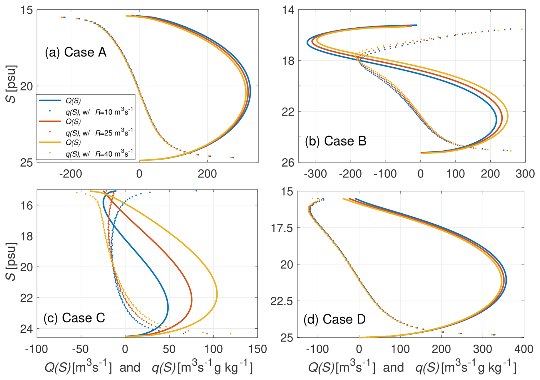
Figure 8 Volume transports Q(S) (solid curves) and exchange profiles q(S) (dotted curves) for cases A, B, C, and D marked with black circles in the parameter space in panels a1 (R = 10 m³ s⁻¹), a2 (R = 25 m³ s⁻¹), and a3 (R = 40 m³ s⁻¹) of Fig. 7. Legend is common to the four panels.

More significant changes occur for phases φ_b≈ 160° for both low and high ratios between M4 and M2 current amplitudes. In Case B (Fig. 8b), characterized by higher M4 vs. M4 amplitude ratios in both current and salinity, inflow (positive q(S) values) is observed at low salinity classes. This is a consequence of the covariance between current and salinity, which governs the integrated salt flux. This phenomenon occurs for this Case B for the three simulated discharges R = 10, 20, and 40 m³ s⁻¹. In Case C, the M4 vs. M2 ratio is smaller, and the exchange transports per salinity class are lower. The salinity range of the q(S) profile widens relative to the M2-only case for all three freshwater discharge values. In this case, inflow is only observed for q(S) over a narrow range of low-salinity classes. Higher freshwater discharge shifts the q(S) profile toward negative (outflowing) values.

3.4 Scope and Limitations

The idealized approach used in this study is simplified and does not take all physical processes affecting exchange flow in estuaries into account. The assumptions made to simplify the equations allow for the construction of a fast and understandable model, but they also limit its scope.

The analysis is restricted to normal, low river flows with zero residual salinity flux. Non-stationarity, which is not taken into account, influences TEF prior and after high-discharge events. Freshwater discharge variability is conditioned by extensive upstream regulation of the drainage basin and is characterized by seasonal, short-duration high-discharge events (days to a few weeks), reflecting the regulation effects of the river basin upstream of the Alcalá del Río dam.

The choice to consider only the most energetic constituent M2 and its main overtide M4 allows for a first reliable and approximate assessment of TEF in estuaries at low computational cost, particularly in cases where no complex high-resolution model is available, or as a benchmark prior to its implementation, highlighting the importance of the covariance between salinity and current. Additionally, this simplified scenario has allowed the effect on TEF of including M4, which accounts for tidal asymmetry, to be evaluated. However, it must be acknowledged that this simplification is a limitation that does not allow for an accurate estimation of TEF capable of capturing its spatio-temporal variability, which is controlled by tidal-fluvial interaction and complex bathymetry. In this regard, a precise estimation of TEF and its variability in the Guadalquivir estuary should be the subject of future research. To this end, other semidiurnal tides should be considered to capture the spring–neap modulation; diurnal constituents which generate diurnal inequality and also contribute to a semidiurnal–diurnal tidal asymmetry (Hoitink et al., 2003); as well as their corresponding compound tides and overtides.

Although it is a common approximation in funneled estuaries, parameterizing the cross-sections using a decreasing exponential is an oversimplification of real bathymetric profiles. Besides, there are lateral and vertical variations of TEF in cross-sections that are not accounted for in this work and should be mentioned. Vertical salinity variations are negligible in an estuary such as the Guadalquivir that is mostly well-mixed, except perhaps in the lower reach near the mouth, where partial stratification may occur. Vertical variability in tidal currents is more significant and, in this regard, the approach adopted in this study may be overestimating total exchange flows. According to Losada et al. (2017), within a monitored water column of ∼ 6 m, differences close to 50 % can occur between the M2 semimajor axis amplitude of the tidal ellipse at the surface and at the bottom. Vertical differences in the M2 tidal ellipse phase do not appear to be significant. Regarding lateral variations, with the available data it is difficult to quantify them. However, there is indirect evidence in the Guadalquivir estuary of their importance (Díez-Minguito et al., 2013) and, therefore, they should be included in future detailed studies with high-resolution numerical models to achieve a more accurate estimation of exchange flows. Lateral separation of the subtidal flow in estuaries occurs due to, e.g., tidal residual currents or lateral variations in the estuarine circulation Burchard et al. (2011); Geyer and MacCready (2014). It is also well-known that local topographic features, such as bends, may have considerable influence on the lateral mixing driven by secondary flows and hence on the salt transport and exchange flows (e.g. Smith, 1976; Lewis and Lewis, 1983; Pein et al., 2018).

Recently, Rummel et al. (2025) studied the salt transport mechanisms in the North German Weser River Estuary using a detailed transport decomposition method applied to a high-resolution numerical model. These authors found that opposing flows often occur between the channel and adjacent shoals in this estuary. Outflow subtidal depth-averaged transport occurs on the shoals, whereas a net inflow occurs on the inner part of the channel. Also, in the bends of the Weser estuary, an outflow is found in the outer part of the bend, whereas in the center of the channel as well as the inner shoals, a residual inflow occurs. In the Guadalquivir estuary, Díez-Minguito et al. (2013) provided indirect evidences of lateral separation of salt fluxes from analysis of observations near the thalweg. These authors noticed that during several months during low river-flows the 2 psu isohaline location (X₂) did not show appreciable variations besides its a weak spring-neap variability. However, there was a persistent net salt influx on the inner part of the channel, thereby suggesting the presence of lateral variations over the cross-section and a compensating net salt outflux on the shoals.

Finally, TEF estimates of incoming and outgoing water volume transports in the lower part of the estuary obtained in this study are about 10 % larger than volume transports inferred from a tidally-averaged Eulerian approach by Reyes-Merlo et al. (2013), who only considered the contribution of the density-driven flow to the exchange. The actual differences from these two different approaches are likely to be larger since the present study only considers the contribution of the M2 tidal constituent to TEF. As noted above, other constituents may potentially enhance tidal salt transport. Díez-Minguito et al. (2013) observed that tidal salt transport is dominant, showing that Stokes transport and tidal pumping are at least one order of magnitude larger than those induced by vertically-sheared currents. Nevertheless, the water column structure in the lower part of the estuary is partially stratified rather than well-mixed, showing the residual horizontal currents an evident vertically-sheared profile (Reyes-Merlo et al., 2013). Semi-analytical model results by Biemond et al. (2024) highlighted the importance of accounting for density-driven flow when estimating salt transport, particularly in this lower part of the estuary. They showed that this transport mechanism cannot be neglected. Salt transport due to density-driven flow interacts with that associated with current–salinity correlations, and both contributions are equally important in the lower part of the Guadalquivir Estuary.

4 Conclusions

An oscillatory exchange flow scenario including the contributions of M2 and M4 current and salinity is applied to the Guadalquivir estuary to estimate Total Exchange Flow (TEF) for the first time at seven cross-sections during low river flow conditions. Estimates are determined combining the analytical approach with high-resolution field measurements of currents and salinity along the main channel. A sensitivity analysis of exchange profiles and volume transports to the inclusion of the M4 constituent to the tidal flow and salinity is performed. The results of this study translated into the following conclusions.

Knudsen-bulk estimates along the main channel using TEF framework decrease upstream in the Guadalquivir estuary. Incoming and outgoing water volume transports are about 10 % larger than previous estimates based on gravitational circulation only. In the middle part of the estuary, incoming TEF bulk volume values below 150 m³ s⁻¹ are obtained. The largest net incoming water volume transport, viz. approx. 300 m³ s⁻¹, is attained at the lower part of the estuary, near where the largest salinity gradient is observed. This value is about 12-fold the normal river flow from the head dam at Alcalá del Río. Its corresponding representative TEF bulk salinity value is 20 psu, whereas the representative value for outflows at the same location is about 16 psu. This is consistent with the the poorly-stratified character of the Guadalquivir estuary, with a mixing completeness larger than 67 % at all cross-sections. The Guadalquivir estuary can be thus rated as of relatively high mixing completeness.

The covariance between M2 salinity and current seems to play a more important role in exchange flow in the Guadalquivir estuary than the effects due to tidal asymmetry. The inclusion of the M4 tidal constituent with regards to the original analysis of the M2(-only) tidal flow produces noticeable effects in salinity values, volume transports and exchange profiles. Knudsen-consistent salinity values increased up to 5 %. At all locations in the estuary, the maxima of the volume transport Q(S) are about 10 % larger when considering the superposition of M2 and M4 constituents.

The inclusion of the M4 yield differences with regard to the only-M2 case in volume transports and exchange profiles, and thus in volume transports, salinities, and salt transports. These differences could be even more significant in other semi-enclosed basins with higher tidal asymmetry than that of the Guadalquivir estuary. The sensitivity analysis shows that the M4 constituent changes magnitude of the exchange flow by salinity class and range of salinities associated to outflows and inflows. Changes in magnitude of the exchange flow due to the M4 inclusion are comparable in magnitude to those produced by changes in along-channel cross-section profile. The larger deviations from the reference case with the M2 term only occur when the ratio between M4 and M2 current amplitudes is larger, and the M4 current phase is closer to 160°. The modified exchange profiles show in that case a remarkable inflow at low salinity classes.

Overall, this study contributes to further understanding TEF in weakly-stratified estuaries. Estimates provided in this work, which are based on a simple tidal oscillatory set of equations and field data from a comprehensive field campaign, could serve as a basis and touchstone for further works with more complex computational models in the Guadalquivir estuary. The low computational cost of the M2+M4 oscillatory exchange flow scenario makes it particularly suitable to be applied systematically (and simultaneously) in a large number of estuaries at a regional scale. This approach allows studying trends in TEF caused by climate-scale changes in freshwater discharges, salinity distribution, and tidal parameters in estuaries.