Climatology and annual cycle of global ocean dissolved oxygen represented by multiple observational gridded products

Ocean dissolved oxygen (O₂) is an essential climate variable crucial for sustaining the marine life; thus, changes of O₂ at various spatiotemporal scales should be quantified and understood. Here, we study the climatology and annual cycle of O₂ at regional to global scales using eight available gridded observational products. These datasets are generated by different groups using different primary data selection, quality control, bias correction, and interpolation methods, including statistical and machine-learning-based mapping methods. A common set of metrics was collaboratively developed by the community of the Gridded Observational Dataset Intercomparison Project-Dissolved Oxygen (GODIP-DO) to facilitate the inter-comparison. We find that global mean O₂ profiles are consistent among all products (±3 µmol kg⁻¹), with the well-established decrease from high surface values to a minimum ∼ 1000 m, and subsequent increase to higher O₂ at depth, although local differences could reach ±25 µmol kg⁻¹ (0–1000 m). The hemispheric O₂ annual cycle correlates strongly with ocean temperature changes, suggesting the key driver of temperature for the O₂ annual cycle. However, there is substantial variation in the global mean 0–100 m O₂ annual cycle, the magnitude ranges from −1 to 0.8 µmol kg⁻¹, with a standard deviation of the datasets of ∼ 0.3 µmol kg⁻¹. Average oxygen minimum zones (OMZ) volume among the products is 80.92 × 10⁶ km³ (±1.95 %) for a 60 µmol kg⁻¹ threshold and 152.00 × 10⁶ km³ (±1.72 %) for a 90 µmol kg⁻¹ threshold. Our results help to depict and understand the spread among the available O₂ gridded datasets.

1 Introduction

Anthropogenic climate change drives ocean warming, increases stratification, and alters ocean circulation (Bindoff et al., 2019). These changes lead to the loss of ocean dissolved oxygen (O₂), namely deoxygenation, because of the changes in the O₂ solubility, ventilation, and deep ocean respiration (Keeling et al., 2010; Schmidtko et al., 2017; Breitburg et al., 2018; Oschlies et al., 2017, 2018; Garcia-Soto et al., 2021). Deoxygenation occurred in most open ocean regions during the mid-20th to early 21st centuries, such as the Mediterranean Sea, tropical oxygen minimum zones (OMZ), and the North Atlantic Subtropical Gyre (Tan et al., 2026), influencing marine ecosystems through resulting biogeochemical feedbacks such as ocean productivity, nutrient cycling, carbon cycling, marine habitat, etc (Levin, 2018; Bindoff et al., 2019). Given its importance, studying O₂ changes at various spatiotemporal scales becomes critical.

Observations and model simulations document a robust decline of the global O₂ inventory, which is a grand challenge for the accurate assessment of deoxygenation (Ito et al., 2017; Schmidtko et al., 2017; Breitburg et al., 2018). For trends, current assessments such as the Intergovernmental Panel on Climate Change (IPCC) Special Report on the Ocean and Cryosphere in a Changing Climate (SROCC) indicates that the open ocean is losing O₂ overall with a decadal variability of 0.3 %–2 % since the 1960s over all ocean depths and of 0.5 %–3.3 % between 1970 and 2010 from the ocean surface to 1000 m, with an expansion of OMZ by 3 %–8 % (Bindoff et al., 2019; Gulev et al., 2021; Zhou et al., 2022). In addition, a recent observational-based assessment by Tan et al. (2026) shows that significant signal emergence of long-term O₂ trends (both deoxygenation and oxygenation) can now be detected across global ocean in a large-scale and deep-reaching pattern since the 1990s, although the regional data uncertainty still needs to be taken into account. These studies reveal substantial uncertainty in quantifying the open ocean O₂ trends, however, there is no dedicated study assessing the available products on O₂ climatology and its annual cycle, which is the key focus of the present study.

The differences among different O₂ products may arise from the instruments/platforms used to obtain O₂ profiles and the data processing techniques including quality control processes, bias correction approaches, vertical interpolation methods, mapping methods (horizontal interpolation), land-ocean masks, and so on. Since the late 19th century, oceanographers have measured ocean O₂ using many observing systems with varying sampling resolutions. The very first observing system includes the chemical titration method developed by Winkler (Ocean Station Data, OSD), which restricted the O₂ observations derived from water samples to several depth levels. Electrochemical and optical sensors for measuring O₂ became prevalent in the 1960s–1970s and are now widely used to make continuous measurements on platforms such as the CTD (Conductivity-Temperature-Depth) profilers. Biogeochemical Argo profiling floats (BGC-Argo) have provided increasing ocean O₂ observation profiles since the early 2000s, and underwater gliders (GLD) and moorings are especially useful for regional oceanography (Gregoire et al., 2021; Gourteski et al., 2024b). The Winkler data are labour intensive with lower sampling resolution, whereas sensor-based measurements have better spatiotemporal resolution, and the proliferation of the BGC-Argo program has dramatically increased O₂ observations.

With the ocean O₂ observations collected using different observing systems, there have been several quality controlled global ocean O₂ observation datasets from different research organizations/groups such as the National Centers for Environmental Information (NCEI) of the National Oceanic and Atmospheric Administration (NOAA) (Garcia et al., 2024; Garcia et al., 2018; Boyer et al., 2018), Shanghai Jiao Tong University (SJTU, Zhou et al., 2022) and the Institute of Atmospheric Physics (IAP) Chinese Academy of Sciences (Gourteski et al., 2024b). These quality controlled observations are then used to construct gridded O₂ data products by filling data gaps with a mapping method where direct observations were not available. The available mapping methods include objective analysis (Garcia et al., 2024), ensemble optimal interpolation with dynamic ensemble (Cheng et al., 2024; Cheng et al., 2017; Cheng and Zhu, 2016), Data Interpolating Variational Analysis (DIVA; Roach and Bindoff, 2023), machine learning techniques (Sharp et al., 2023; Ito et al., 2024; Huang et al., 2023; Liu et al., 2025), and geostatistical regression (Zhou et al., 2022).

All the previously mentioned instrumental data have measurement errors and biases, and the data processing techniques are imperfect, leading to uncertainty in representing the O₂ climatological mean state and its annual variation. A systematic multi-product intercomparison at regional to global scales could serve as the primary tool to assess the robustness of our observational understanding and to quantify the spread in current climatological representations. The spread among different datasets includes all uncertainty factors and is different from the recent single-factor assessment of Ito et al. (2025) who focused solely on mapping methods. In particular, we employed eight ocean O₂ climatology products, covering statistical and machine-learning-based mapping methods whereas Ito et al. (2025) included statistical mapping methods only. Our analysis includes the gridded O₂ dataset from IAP (Gourteski al., 2024), World Ocean Atlas 2023 (hereafter, WOA23; Garcia et al., 2024) and World Ocean Atlas 2018 (hereafter, WOA18; Garcia et al., 2018; Boyer et al., 2018) by NCEI, a machine-learning-based data product by Sharp et al. (2023) (Gridded Ocean Biogeochemistry from Artificial Intelligence, hereafter, GOBAI; Sharp et al., 2023), two data products based on DIVA by Roach and Bindoff (2023) (hereafter, RB; Roach and Bindoff, 2023) and Global Ocean Data Analysis Project (hereafter, GLODAP; Lauvset et al., 2016), a geostatistical gridded O₂ dataset from SJTU (Zhou et al., 2022), and a machine-learning-based data product (hereafter, Jingwei; Lu et al., 2024).

The rest of the paper is organized as follows. The gridded datasets and methods employed in the study are presented in Sect. 2. In Sect. 3, the results of depicting the characteristics and assessing the spread of O₂ climatology and annual cycle for different products are introduced. The analysis related to OMZ distribution is also presented in Sect. 3. The results of the study are summarized and discussed in Sect. 4.

2 Datasets description

We used eight O₂ gridded products (IAP, WOA23, WOA18, GOBAI, RB, GLODAP, SJTU, and Jingwei) that are different in many aspects including the instruments to get raw O₂ profiles and also the data processing techniques, such as quality control and bias correction approaches, vertical interpolation methods, mapping methods, land-ocean masks, and so on (Table 1).

The observations used by IAP, WOA23, WOA18, RB, SJTU, and Jingwei are mainly from WOD (World Ocean Database, Boyer et al., 2018; Mishonov et al., 2024) and BGC-Argo. Observations from GLODAP are also used in GOBAI product. The IAP, WOA23, WOA18, and GOBAI datasets include monthly climatology, and the remaining four data products (RB, GLODAP, SJTU, and Jingwei) only provide the annual mean climatology. So, analyses related to the annual variation of the global ocean O₂ and the annual cycle are restricted to the four datasets with monthly climatology (IAP, WOA23, WOA18, and GOBAI). The gridded data products of IAP, WOA23, WOA18, RB, GLODAP, and Jingwei reach the ocean bottom of about 5500 m/6000 m. GOBAI and SJTU only cover the top 2000 m. The horizontal resolution of the data product of RB and SJTU is 0.5° × 0.5° and 2° × 2°, respectively, and all the other six products are at a resolution of 1° × 1°. The horizontal space coverages of all the datasets are also slightly different. The space coverage of the GOBAI data is limited by the distribution of the temperature and salinity data product on which it is based, so GOBAI only covers 64.5° S–79.5° N of the open ocean (O₂ in the coastal regions and oceans with complex topography are not reconstructed). The mapping method for WOA18 and WOA23 is based on objective analysis and that for IAP is the ensemble optimal interpolation with dynamic-ensemble. GLODAP and RB both adopt the DIVA method to generate gap-filled fields. SITU develops the geostatistical regression interpolation method. The feed-forward neural network and the spatio-temporal graph hypernetwork are used for the machine learning process of the GOBAI and Jingwei data products, respectively (Table 1). To illustrate the spatiotemporal characteristics of the observation profiles, the spatial distribution and annual number of the three main observation platforms (OSD, CTD, BGC-Argo) for 1960–2024 are shown in Fig. 1.

Table 1 Global ocean O₂ gridded datasets employed in the comprehensive inter-comparison of the climatology (EnOI-DE: ensemble optimal interpolation with dynamic-ensemble; OA: objective analysis; ML: machine learning; GR: geostatistical regression).

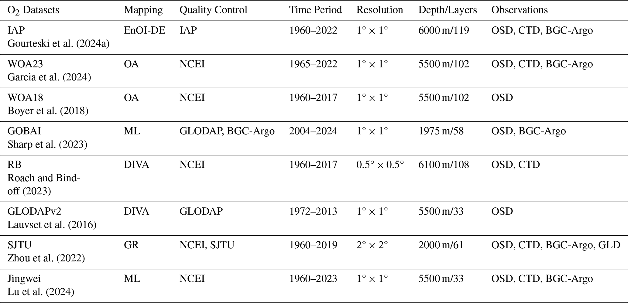
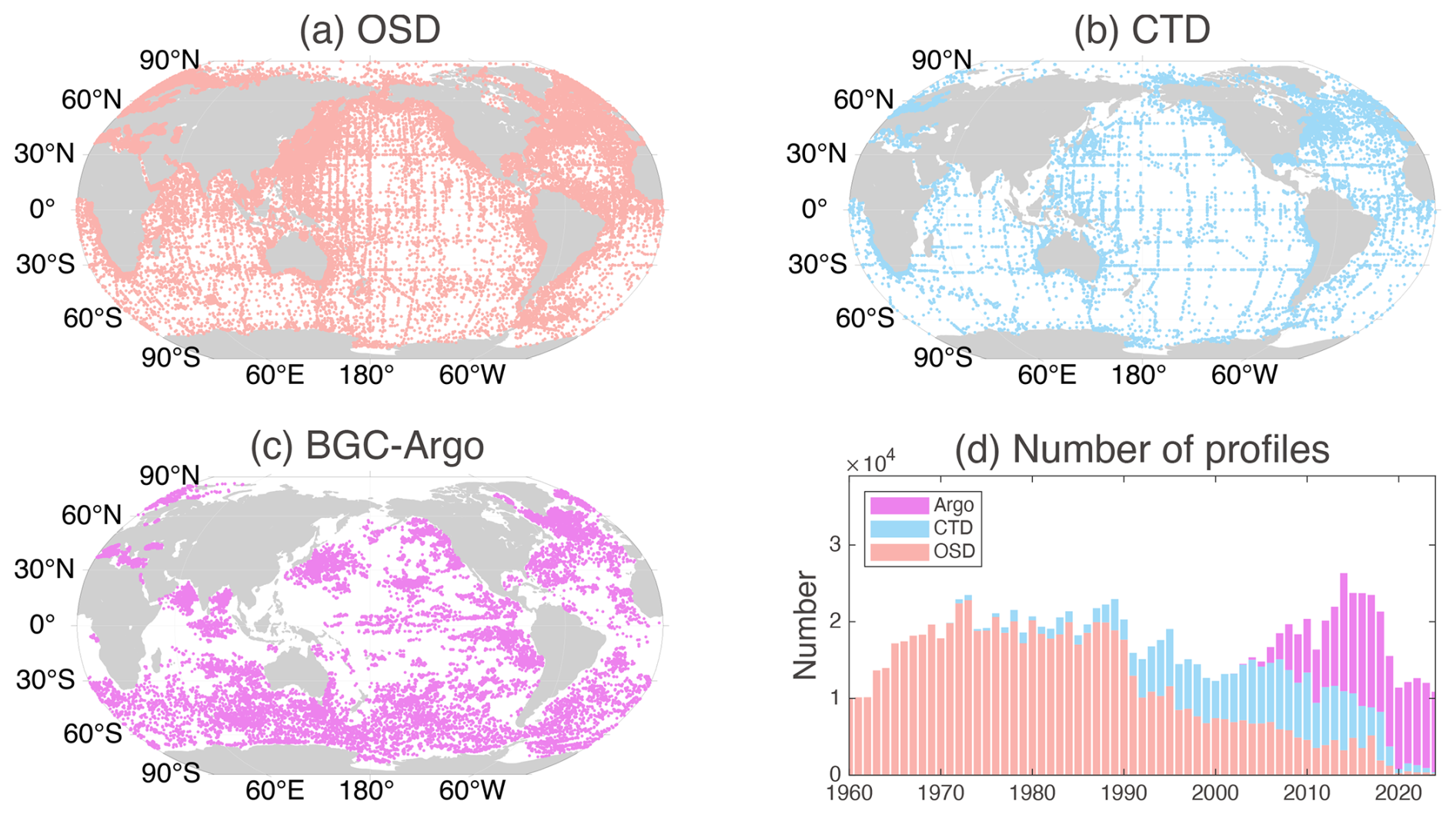
Figure 1 Spatial distribution ((a) OSD, (b) CTD, (c) BGC-Argo) and annual number (d) of observation profiles.

This study used a common ocean mask, which is defined as ocean grid points with all data products available. The common land-ocean masks for the layers of 100 and 2000 m are presented in Fig. 2 and the common masks for the other layers (1000, 3000, 4000, and 5000 m) are available in Fig. S1 in the Supplement. This will be a uniform comparison and remove the impacts of different data coverage on the results. The datasets of RB and SJTU were interpolated to a common 1° × 1° resolution as all the other datasets to facilitate the comparison, but the interpolation has a negligible impact on the results presented in this work (less than 0.01 % for the global mean O₂).

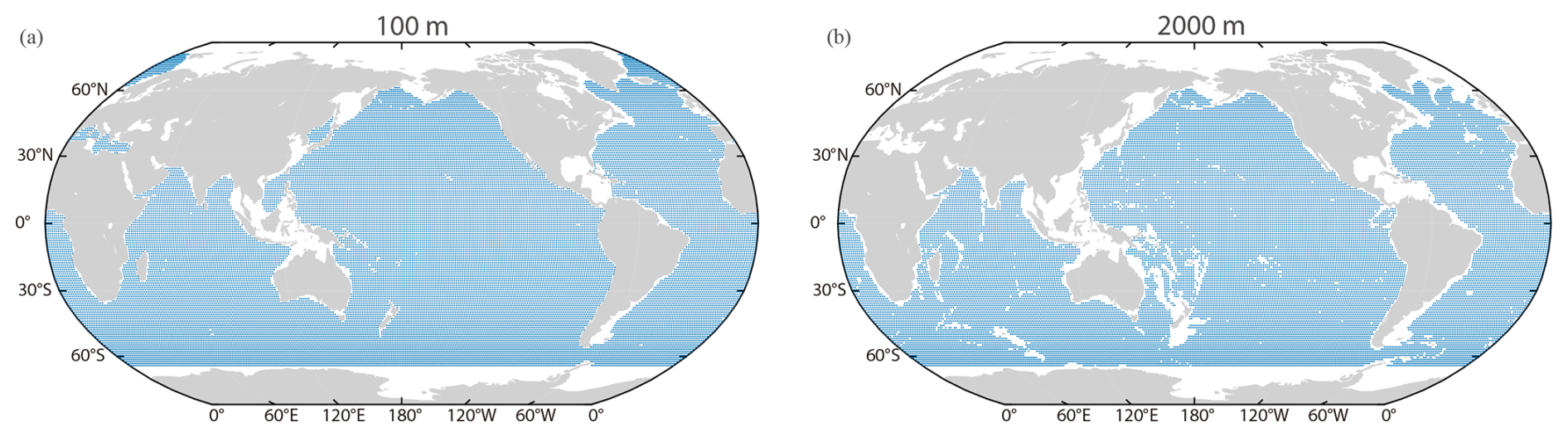
Figure 2 Grid point distribution of the common land-ocean mask for the layers of 100 m (a) and 2000 m (b).

3 Results

3.1 Global mean O₂

The global area-weighted mean O₂ profile is first presented in Fig. 3a, showing a well-established vertical structure and a good consistency among all products. O₂ is higher near the surface than in the deeper ocean because of the gas exchange with the atmosphere and photosynthesis. The O₂ reaches the lowest value at ∼ 1000 m because of the respiration and limited O₂ supply from the surface. The O₂ increases from ∼ 1000 m to the deep ocean (∼ 5000 m) because of the weaker respiration and the intermediate, deep, and bottom water formation that supplies higher O₂ water into the deep layers, where cold, dense surface water sinks, and is then distributed globally by deep ocean currents, slowly losing O₂ along its centuries-long journey (Musan et al., 2023).

To better quantify the differences among the datasets, we take the difference between all seven other data products (WOA23, WOA18, GOBAI, RB, GLODAP, SJTU, and Jingwei), and IAP data (Fig. 3e–h). The differences are mostly within ±3 µmol kg⁻¹ among all the datasets with a common land-ocean mask from ocean surface to 5500 m, except that the differences for SJTU and Jingwei range between −6 and 5 µmol kg⁻¹ for the upper 200 m. The differences are comparable to the magnitude of O₂ anomaly, whose semi-decadal median is within ±10 µmol kg⁻¹ within major ocean basins (Schmidtko et al., 2017).

There is a negative offset between GOBAI and IAP ($\sim -\mathrm{2}$ µmol kg⁻¹). The differences between WOA18, RB, and IAP are positive. One possible reason for these differences is that different data products construct climatologies using data from different time periods with different resolutions. The SJTU climatology uses CTD, OSD, BGC-Argo, and additional GLD data, then interpolates them at coarser 2° × 2° resolution. The GOBAI climatology is reflective of a more recent period compared to the other datasets (2004–2024), which might at least partly explain the negative difference between GOBAI and IAP (where data from 1960–2022 are used). Because of the general deoxygenation trend, a “newer” climatology is expected to show less global mean O₂ than an “older” climatology. IAP is close to WOA23 at the upper 2000 m within 1 µmol kg⁻¹, which is reasonable because both IAP and WOA23 used bottle (OSD), CTD, and delayed-mode BGC-Argo data using the same 1° × 1° data resolution, and they have similar time coverage of data used to generate climatology (IAP, 1960–2022, and WOA23, 1965–2022).

Below 2000 m, there is an offset between IAP and WOA23: WOA23 O₂ is 0.2–0.6 µmol kg⁻¹ higher than IAP. Possible explanations may be the differences in quality control and mapping methods. Another possibility is the “jump” around 2000 m of IAP minus WOA23. It is common to have a discontinuity around 2000 m because of the big differences in data amount and data distributions at upper and deeper layers (observations are concentrated in the upper ocean and most of the BGC-Argo data are in the upper 2000 m). Differences in infilling the empty grid nodes during the mapping procedure may also play a significant role in deep ocean layers where the number of observation data is severely limited. Results of applying different mapping methods to the same in situ datasets suggest that mapping methods may contribute to a difference of less than ±1 µmol kg⁻¹ for the 0–5500 m area-weighted averaged O₂ (Ito et al., 2025). And using two different quality control processes and the same mapping procedure yields a difference of only ±0.5 µmol kg⁻¹ (Ito et al., 2025).

The mean O₂ profiles and the differences between datasets for major ocean basins (Pacific, Atlantic, Indian) are calculated separately and presented in Fig. 3b–d and f–h. The differences are mostly within ±4 µmol kg⁻¹ among all the datasets for the Pacific and Indian Oceans, except that the difference for Jingwei ranges between −8 and 2 µmol kg⁻¹ for the upper 200 m in the Pacific Ocean (Fig. 3f). The mean O₂ profiles for the Atlantic Ocean show more notable differences compared to other ocean basins (Fig. 3c), including that the mean O₂ profile of SJTU data shows a difference of −10 to −5 µmol kg⁻¹ for the depth of 1000–2000 m, while the differences of all the other datasets are constrained to −5 to 5 µmol kg⁻¹ from ocean surface to the depth of 5500 m (Fig. 3g). For the Atlantic Ocean, the mean O₂ reached the minimun at the depth of ∼ 500 m (Fig. 3c), which is much shallower than the O₂ minimun layers for the Pacifc and Indian Oceans (∼ 1000 m, Fig. 3b, d), possibly due to a combined effect of the formation, transport, and mixing process of the North Atlantic Deep Water (NADW), the ventilation processes such as Atlantic Meridional Ocean Circulation (AMOC), and so on (Levin, 2018; Koelling et al., 2022; Musan et al., 2023; Ruhl et al., 2025).

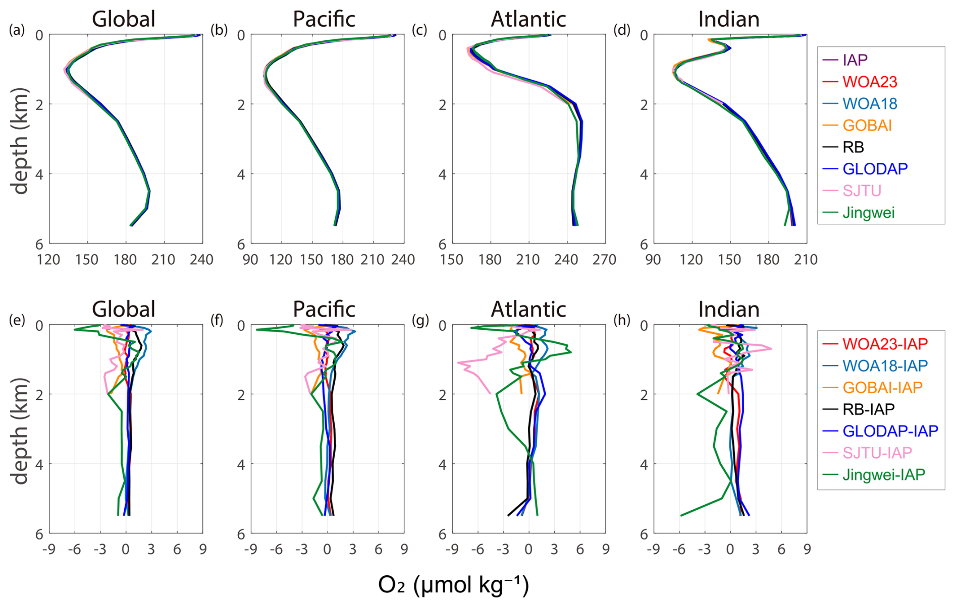
Figure 3 Area-weighted mean O₂ climatology (a–d) and difference (e–h) relative to the IAP for the Global, Pacifc, Atlantic, and Indian Oceans from ocean surface to 5500 m with a common ocean mask for different ocean basins in units of µmol kg⁻¹. The subplots for O₂ climatology (a–d) use different scales.

3.2 Zonal mean structure

The global zonal mean O₂ concentration of the eight datasets for the upper 1000 m shows consistency for the zonal structure (Fig. 4a). There is a minimum of mean O₂ levels around the tropical regions for all the datasets, associated with a shoaling of the tropical and subtropical thermocline depth (Deutsch et al., 2011) and the presence of the tropical upper ocean OMZ. The differences in the global zonal mean O₂ for the upper 1000 m between the seven data products (WOA23, WOA18, GOBAI, RB, GLODAP, SJTU, and Jingwei) and IAP are shown in Fig. 4b. The differences in zonal mean 0–1000 m averaged O₂ are mostly within ∼ 5 µmol kg⁻¹. The zonal mean O₂ difference between IAP and WOA23 is the smallest, which is generally within ∼ 1.5 µmol kg⁻¹. The zonal mean of GOBAI is generally lower than that of IAP, especially in the Northern Hemisphere, which may imply stronger deoxygenation trends in the Northern Hemisphere, as the GOBAI climatology baseline is newer than that of IAP. The zonal mean of the RB dataset is higher than that of IAP by ∼ 0.78 µmol kg⁻¹ on average, consistent with the positive offset shown in Fig. 3. Jingwei dataset has the strongest differences from IAP and other products, showing a notable zonal fluctuation.

The results for the depth layers 0–600 and 0–2000 m (Fig. S2) show similar variation pattern to the depth layer 0–1000 m. The differences in the global zonal mean O₂ between data products are mostly within ∼ 5 µmol kg⁻¹ for 0–600 m and within ∼ 3 µmol kg⁻¹ for 0–2000 m (Fig. S2b, d). For 0–600 m, the zonal mean O₂ difference between IAP and WOA23 is the smallest and Jingwei shows the strongest differences from IAP and other products. For 0–2000 m, the depth average makes the difference between datasets much smaller. Jingwei still shows relatively large discrepancy from the other datasets in the regions around 60° N and the equator. Within the latitude range 20–50° S where all other data products show the best agreement, Jingwei exhibits a significant deviation of ∼ 5 µmol kg⁻¹ from the rest.

However, the zonal mean O₂ concentration for 0–100 m (Fig. 4b) shows a relatively distinct pattern. The zonal mean O₂ decreases linearly with the decrease of latitude for all the datasets, except that for the high latitude range 60–80° S, the zonal mean O₂ profiles maintain a relatively stable value and the estimations between different data products vary to an extent of ∼ 20 µmol kg⁻¹ (Fig. 4d), which illustrates the relatively higher uncertainty in the data reconstruction in this high latitude range.

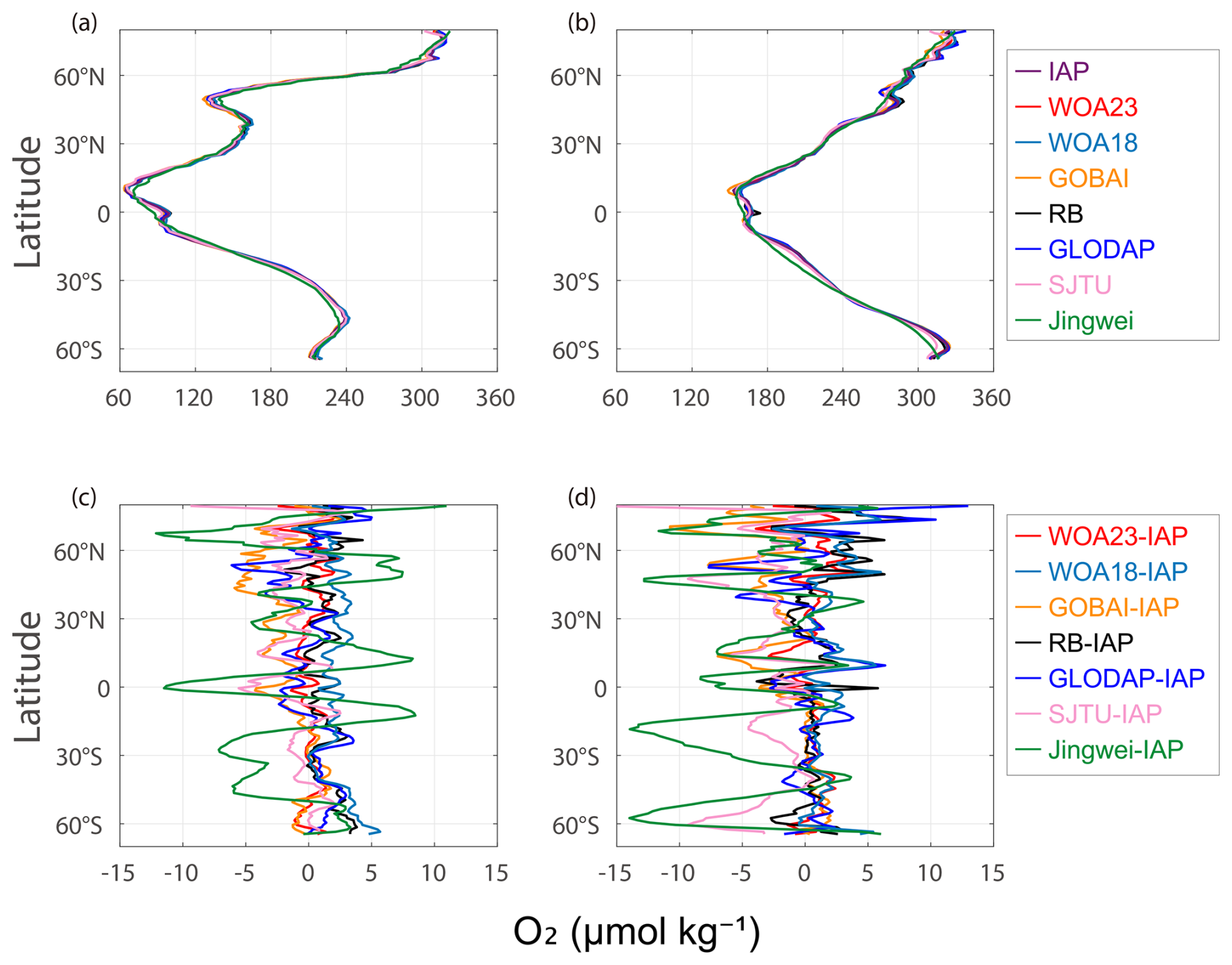
Figure 4 Global zonal mean O₂ concentration and differences for 0–1000 m (a, c) and 0–100 m (b, d) (unit: µmol kg⁻¹).

3.3 Spatial pattern

The spatial distribution of the upper 1000 m mean O₂ and the difference between IAP and six other datasets is shown in Fig. 5a–m. The dataset of Jingwei is not included because the spatial maps are not currently available. The difference of the 0–1000 m mean O₂ is mainly within the magnitude of ∼ 15 µmol kg⁻¹, which shows substantial local differences even though their differences are relatively small when averaged globally (∼ 3 µmol kg⁻¹, Fig. 3). The mean O₂ of the GOBAI dataset is generally lower than IAP for 0–1000 m (Fig. 5f), consistent with the conclusions from the previous comparisons. There are bigger differences located in the regions such as the subpolar North Pacific, the Southern Ocean fronts, and the eastern Pacific regions close to OMZ boundaries, where the strong spatial O₂ gradient, makes the reconstruction sensitive to the mapping process and data distribution (Ito et al., 2025). GOBAI, SJTU, and GLODAP show a negative difference ($\sim -\mathrm{15}$ µmol kg⁻¹) compared to IAP for the upper 1000 m mean O₂ in most of the north and equatorial Pacific Ocean, and equatorial Atlantic Ocean. WOA23 and GOBAI show a similar pattern of difference in the Indian and Pacific Oceans: more positive offsets in the eastern Pacific/Indian Oceans and negative offsets in the western Pacific/Indian Oceans. For the two generations of WOA products, the difference between WOA23 and IAP is more negative globally than the difference between WOA18 and IAP, likely due to the use of more recent data in WOA23. SJTU exhibits a distinct pattern of differences, with substantial negative differences occurring in the tropics.

The spatial map of the spread of the upper 1000 m mean climatological O₂ among all the datasets except Jingwei is presented in Fig. 5n. The spread here is defined as the maximum absolute value of the differences between all the other products and IAP. The spread is within 12 µmol kg⁻¹ in most of the ocean areas, with the largest spread reaching 25 µmol kg⁻¹ where strong spatial O₂ gradients exist. The spread is generally lower in the Southern Hemisphere than in the Northern Hemisphere, in contrast to the fact that there are more observations in the North. This might be related to three issues: (1) A common error in the mapping method, where the spatial interpolation generates over-smoothed or similar-biased fields in the Southern Hemisphere; (2) the variability is lower in the Southern Hemisphere than in the Northern Hemisphere, which reduces the reconstruction errors in the Southern Hemisphere; (3) the deoxygenation trends are higher in the Northern Hemisphere than in the Southern thus the spread reveals the O₂ level at different periods.

The exact reason can be explored with single-factor reconstruction experiments such as those performed by Ito et al. (2025), which use the same input data but different mapping methods to isolate the impact of mapping on climatology reconstruction. Further analyses are required, but it is useful to know the differences between the products. When comparing the depth-mean O₂ between the eight datasets we adopted here which didn't distinguish different impact factors in the process of generating gridded data products and aimed to illustrate a comprehensive discrepancy, the difference for all the datasets for 0–300 m is within ±25 µmol kg⁻¹ and the spread is up to 35 µmol kg⁻¹ (Fig. S3). The regions of high variability mainly locate in the tropical and East Pacific, subpolar North Pacific and Southern Ocean fronts where there are strong spatial O₂ gradients. However, when using the same quality-controlled observational data as input and constraining the impact on data reconstruction to only the mapping method, the difference of the mapped O₂ concentration between different mapping methods is within ±10 µmol kg⁻¹ for 0–300 m (Ito et al., 2025). The overall difference between the data products is more than two times of the difference constrained to a single factor of the mapping method, indicating that the other factors, such as the quality control technique, bias correction, vertical interpolation, and so on, also contribute to the uncertainty source to a large extent. Further analyses are required to assess and quantify the impact of every individual procedure on the whole process of O₂ data reconstruction, but it is useful to know the differences between the data products as a start.

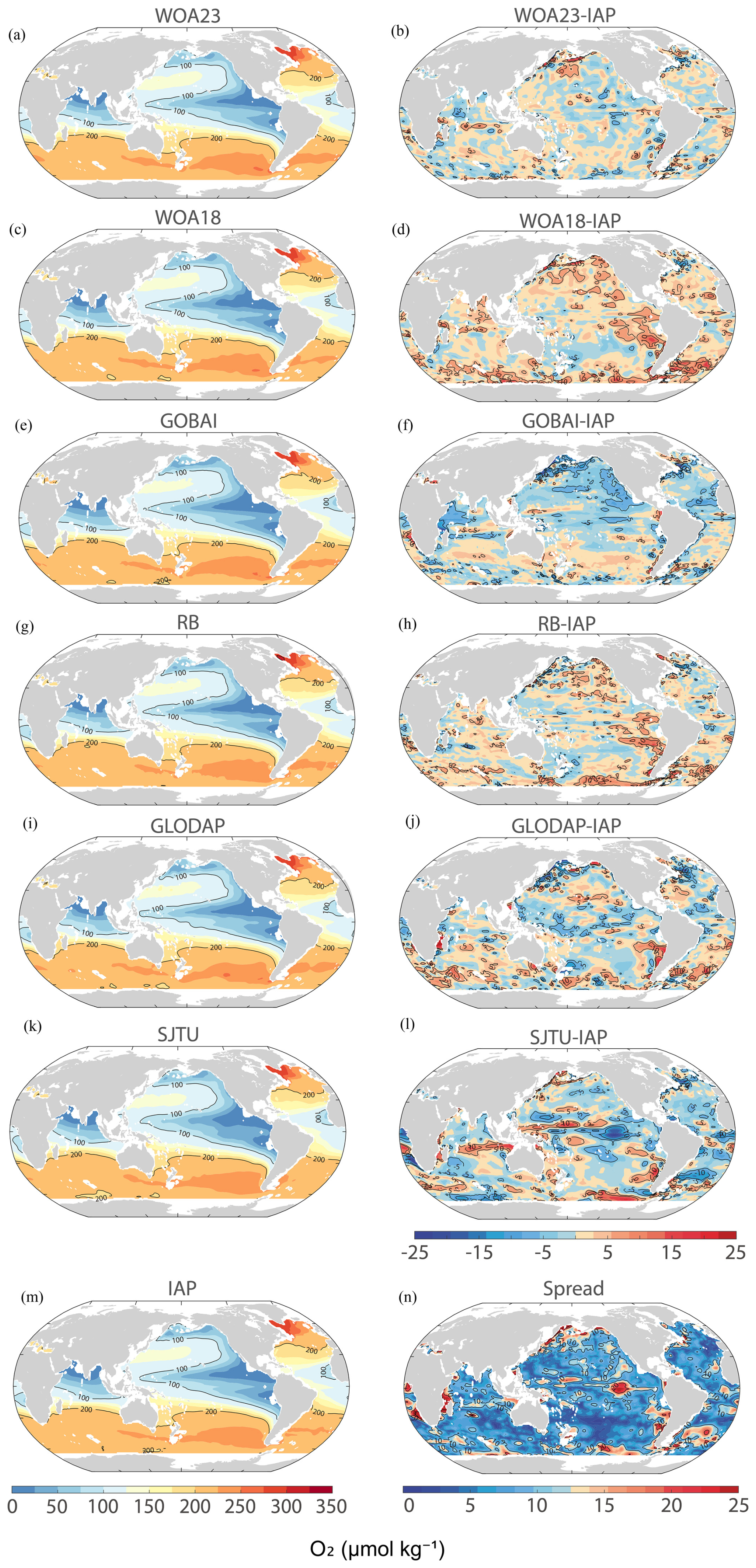
Figure 5 The spatial patterns of the upper 1000 m climatological mean O₂ concentration (unit: µmol kg⁻¹). (a) WOA23, (b) WOA23-IAP, (c) WOA18, (d) WOA18-IAP, (e) GOBAI, (f) GOBAI-IAP, (g) RB, (h) RB-IAP, (i) GLODAP, (j) GLODAP-IAP, (k) SJTU, (l) SJTU-IAP, (m) IAP, (n) Spread is calculated as the difference of the upper 1000 m climatological mean O₂ among the datasets.

3.4 Annual cycle

The annual cycle of the four products that provide a monthly climatology (IAP, WOA23, WOA18, and GOBAI) is presented in Fig. 6 for the 0–100, 100–600, and 600–1500 m, and for Northern and Southern hemispheres, respectively calculated by the monthly anomalies derived by subtracting the annual mean climatology of every data product respectively. The annual cycle of the 0–100 m temperature for northern and southern hemispheres is also calculated using the gridded temperature climatology product of IAP (Cheng et al., 2024). The magnitude of the O₂ seasonal cycle, defined as the maximum amplitude of the annual variation, is greatest near the surface and decreases with depth. Specifically, it is approximately 6 µmol kg⁻¹ for the 0–100 m layer and 2 µmol kg⁻¹ for the deeper layer (100–600 m). The reduced annual cycle with depth is associated with stronger annual variations of ocean temperature, wind-driven ventilation, and biological processes in the upper ocean compared to the deep ocean.

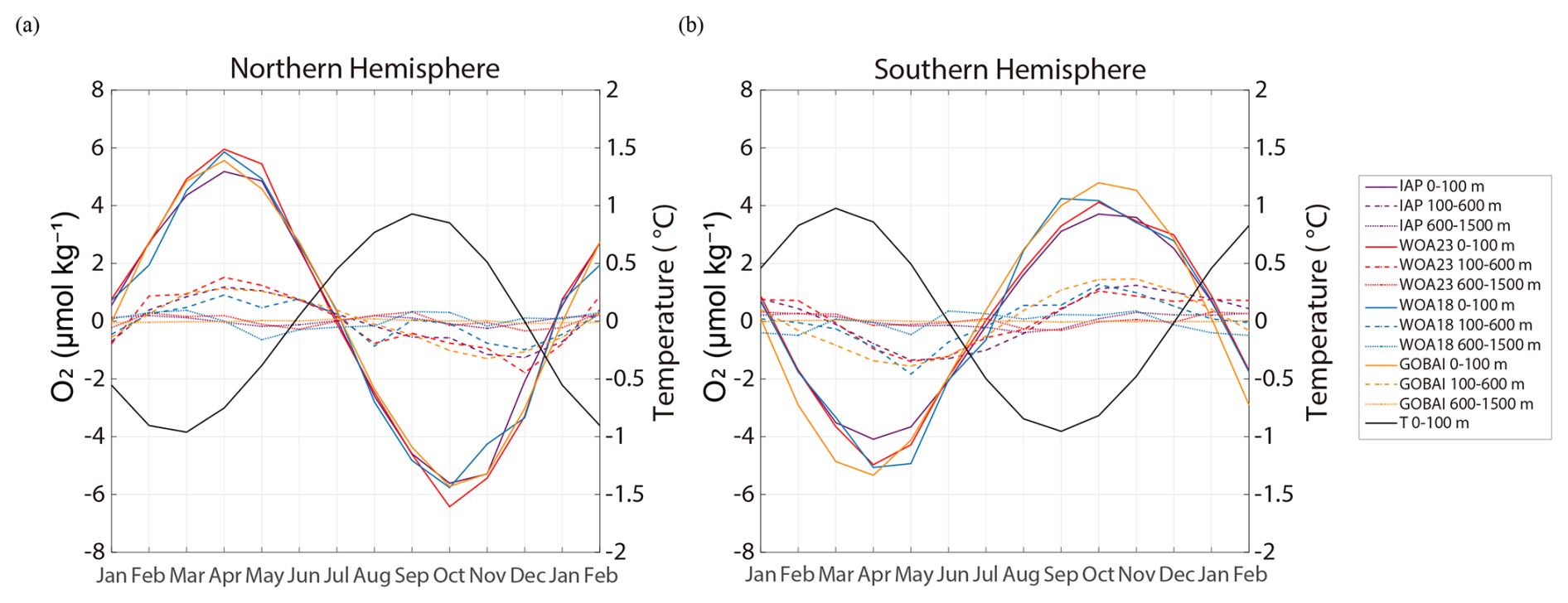
Figure 6 Annual variation of the (a) Northern Hemisphere and (b) Southern Hemisphere global mean O₂ for IAP, WOA23, WOA18, and GOBAI datasets.

The appearance time of maximum (April) and minimum (October) O₂ levels in the northern hemisphere are consistent among the four datasets for 0–100 m global mean O₂. Moreover, the O₂ maximum in the depth layer in the northern and southern hemispheres for 0–100 m lags about one month behind the temperature change, reflecting that besides the dominant thermal induced increase in O₂ solubility, some physical/biological processes also impact the concentration of ocean O₂ (Garcia et al., 2005b; Wang et al., 2022). For the northern hemisphere, the annual variation of the subsurface 100–600 m layer also shows a pattern of annual cycle with the maximum (April) and minimum (December) similar to the surface 0–100 m layer, indicating that the O₂ annual cycle could penetrate to the deeper layer of ∼ 600 m. It is primarily due to the mechanisms including climatological winter mixed layer deepening, which ventilates the subsurface, and seasonal thermocline dynamics coupled with organic matter remineralization (Stramma et al., 2010). For the southern hemisphere, similar patterns also exist.

Although the two hemispheric O₂ annual cycles can be well-defined, the global mean is more subtle, as different products show large differences in patterns of the global mean annual cycle (Fig. 7). It appears that global 100–600 m O₂ annual cycles are more consistent across data products than 0–100 m, probably associated with noiser data and more natural variability near the sea surface. For global 100–600 m O₂, all datasets suggest an O₂ reduction from March to September and an increase from October to February, consistent with the Southern Hemisphere changes (Fig. 7b versus Fig. 6b). The magnitude of the global 0–100 and 100–600 m annual cycle ranges from −1 to 0.8 µmol kg⁻¹ for the four datasets, but the standard deviations among the four datasets are ∼ 0.3 µmol kg⁻¹ (0–100 m) and ∼ 0.2 µmol kg⁻¹ (100–600 m), indicating a similar level of signal and noise (Fig. 7).

Figure 7 Global annual variation of the (a) 0–100 m and (b) 100–600 m global mean O₂ for IAP, WOA23, WOA18, and GOBAI datasets.

The annual cycle of O₂ anomalies shows a distinct spatial pattern (0–100 m mean O₂, April versus October, Fig. 8). The anomalies are calculated by subtracting the annual mean from the monthly climatologies for the four datasets (IAP, WOA23, WOA18, and GOBAI) respectively. In April, the O₂ anomalies of 0–100 m in most of the northern hemisphere are positive, and they turn negative in October. The tropical ocean annual cycle is not easily defined, as many regions have semi-annual variability. Different products exhibit a consistent pattern of change, whereas the detailed structures are quite distinct. In general, WOA23 and WOA18 have more patchy characteristics than IAP and GOBAI, likely related to the mapping methods employed by each: WOA uses an anti-distance weighted function to interpolate the field; on the other hand, IAP uses model simulations to provide covariance and GOBAI takes advantage of correlations between O₂ and temperature and salinity, both building physical ocean properties into the reconstruction.

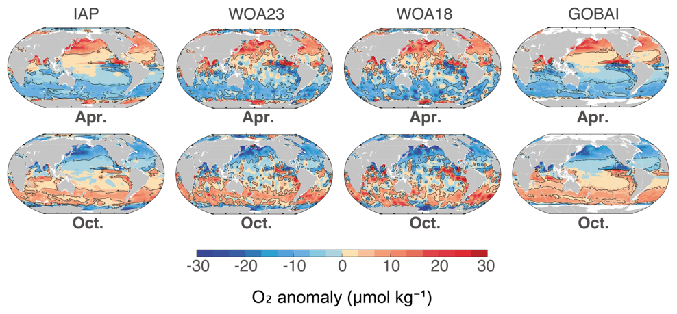
Figure 8 Spatial distribution of the O₂ anomaly (0–100 m) for the IAP, WOA23, WOA18, and GOBAI climatology.

The zonal mean structure of the annual cycle is shown in Fig. 9, and all the datasets show similar annual cycle patterns with some difference in smoothness and magnitude for both 0–100 and 100–600 m mean O₂. For 0–100 m, the largest seasonal changes occur in the extra-tropics in the 30 to 60° N belts of the Northern hemisphere. In the Southern hemisphere, the largest seasonal changes occur in the latitudinal band centered near 40° S. For both 0–100 and 100–600 m, the phase transitions occur around July and January for all datasets, which are consistent with the annual variation analysis in Fig. 6. The phase change of O₂ lags about one month behind the temperature change (June and December as shown in Fig. S4), reflecting that some physical/biological processes also impact the concentration of O₂ besides the dominant thermally induced increase in O₂ solubility. Semi-annual cycles near the equator are visible in the upper ocean for almost all products. There is a distinction of the annual cycle at about 10° N, corresponding to the location of the intertropical convergence zone (ITCZ) (Garcia et al., 2005b).

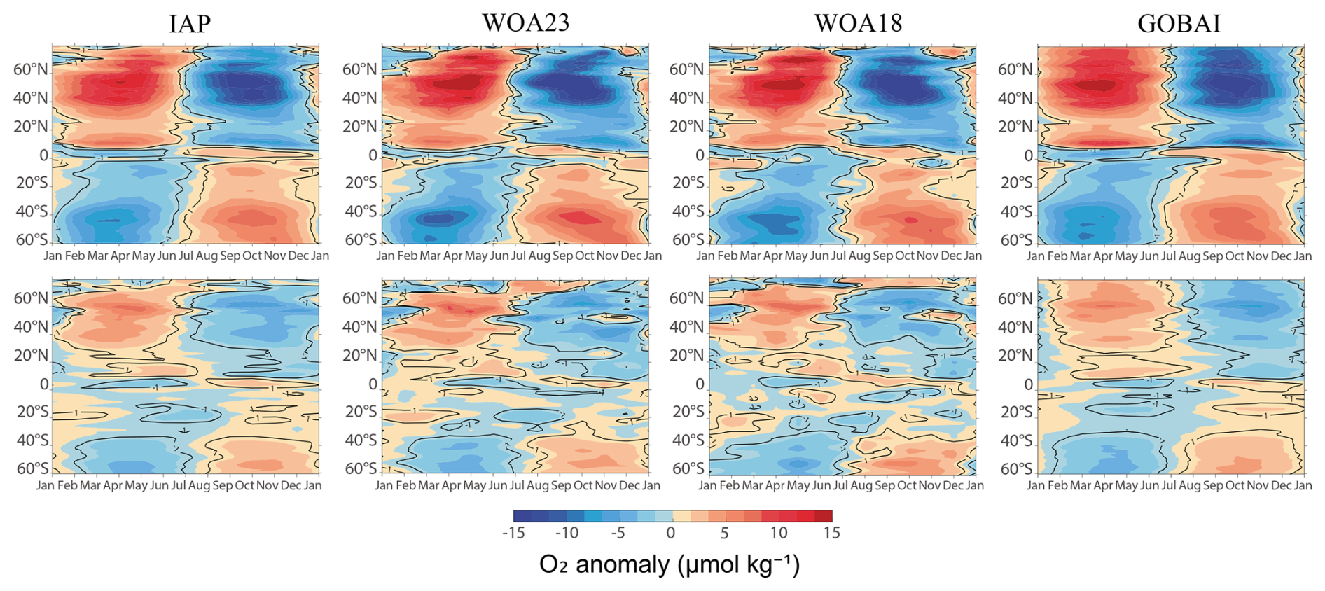
Figure 9 Zonal mean annual cycles for 0–100 m (upper) and 100–600 m (lower) for different data products (IAP, WOA23, WOA18, and GOBAI).

The zonal mean annual cycles of solubility and Apparent Oxygen Utilization (AOU) of different data products for 0–100 and 100–600 m are shown in Fig. 10. The solubility is calculated using the gridded temperature and salinity products of IAP (Cheng et al., 2024) following the Garcia and Gordon (1992) method. Generally, the zonal 0–100 m O₂ seasonal cycle is mainly dominated by the solubility, whereas the AOU dominates the 100–600 m O₂ pattern.

For 0–100 m, the AOU seasonal cycle in the mid-latitude is about two to three months lagging that of the temperature/solubility seasonal variation (Figs. 6, 10, S4). Within 20–60° N, the zonal mean AOU anomaly of 0–100 m is mostly negative from March to August. The phase transition of AOU occurs in March, which corresponds to the temperature minimum/solubility maximum. And AOU reaches a minimum in about May/June, corresponding to the phase transition of the zonal mean temperature/solubility anomaly (Figs. S4, 10). A possible explanation is from the combined impacts of biological and physical processes (Garcia et al., 2005a). The spring phytoplankton bloom lags the onset of temperature increase (starting in March) because phytoplankton proliferation requires sufficient light from increasing spring insolation and nutrient entrainment due to a shallower mixed layer (Martin, 2012). And the net community production (NCP, the difference between gross community photosynthesis and community respiration) reaches a maximum in about May (Wang et al., 2022). The solubility reaches a minimum in September, which corresponds with the phase change of AOU. And the maximum of AOU lags about two months behind the temperature maximum/solubility minimum, which is also a combined effect of the prolonged response time of biological processes and the physical processes possibly induced by the deepening autumn mixed layer. The situation in 20–60° S is similar to 20–60° N for 0–100 m, mainly with the signs reversed. For 100–600 m, the annual variation in temperature/solubility is relatively small, and the pattern of AOU variation dominates, with the underlying processes requiring further investigation.

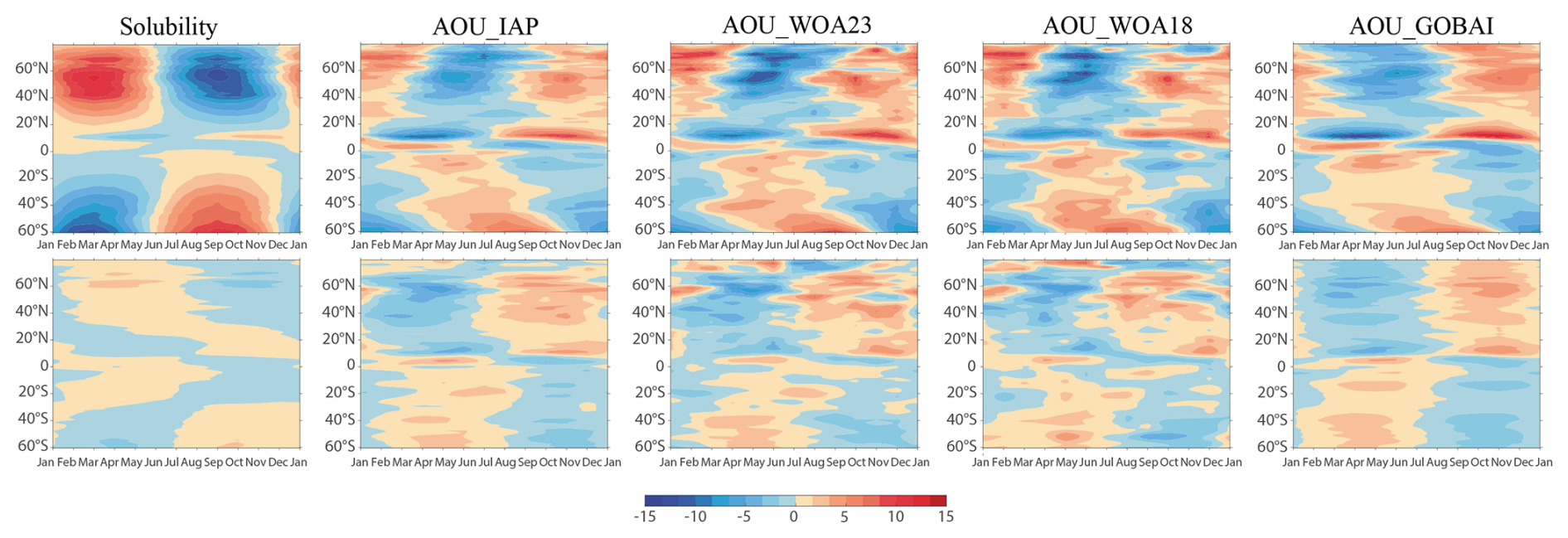
Figure 10 Zonal mean annual cycles of the solubility and AOU anomaly of different data products (AOU_IAP, AOU_WOA23, AOU_WOA18, and AOU_GOBAI) for 0–100 m (upper) and 100–600 m (lower) (unit: µmol kg⁻¹).

To assess the patterns of annual cycle regionally, the zonal mean structures of the annual cycle for different ocean basins are shown in Figs. S5–S7. Distinct seasonal changes exist in the Pacific, Atlantic and Indian Oceans. The annual cycle patterns for the Pacific and Atlantic Ocean coincide with the global O₂ annual cycle both for the 0–100 and 100–600 m layers closely. For the Indian Ocean, there are larger seasonal changes in the latitude range of ∼ 10–20° N for 0–100 m than the Pacific and Atlantic Oceans. The annual variations of the mean O₂ for three major ocean basins (Pacific, Atlantic, Indian) for 0–100 and 100–600 m are shown in Figs. S8–S10, and also for the North and South Pacific/Atlantic, respectively, in Figs. S11–S12. The magnitude of the O₂ seasonal cycle is greatest in the Atlantic Ocean (∼ 3 µmol kg⁻¹) for the 0–100 m layer, which corresponds to a magnitude of ∼ 6 µmol kg⁻¹ in the North Atlantic and ∼ 4 µmol kg⁻¹ in the South Atlantic. The minimum and maximum O₂ levels (−4 to 6 µmol kg⁻¹) and also occurrance time (July/October) of WOA18 for 0–100 m differ the most from those of the other three datasets in the South Atlantic (Fig. S12b).

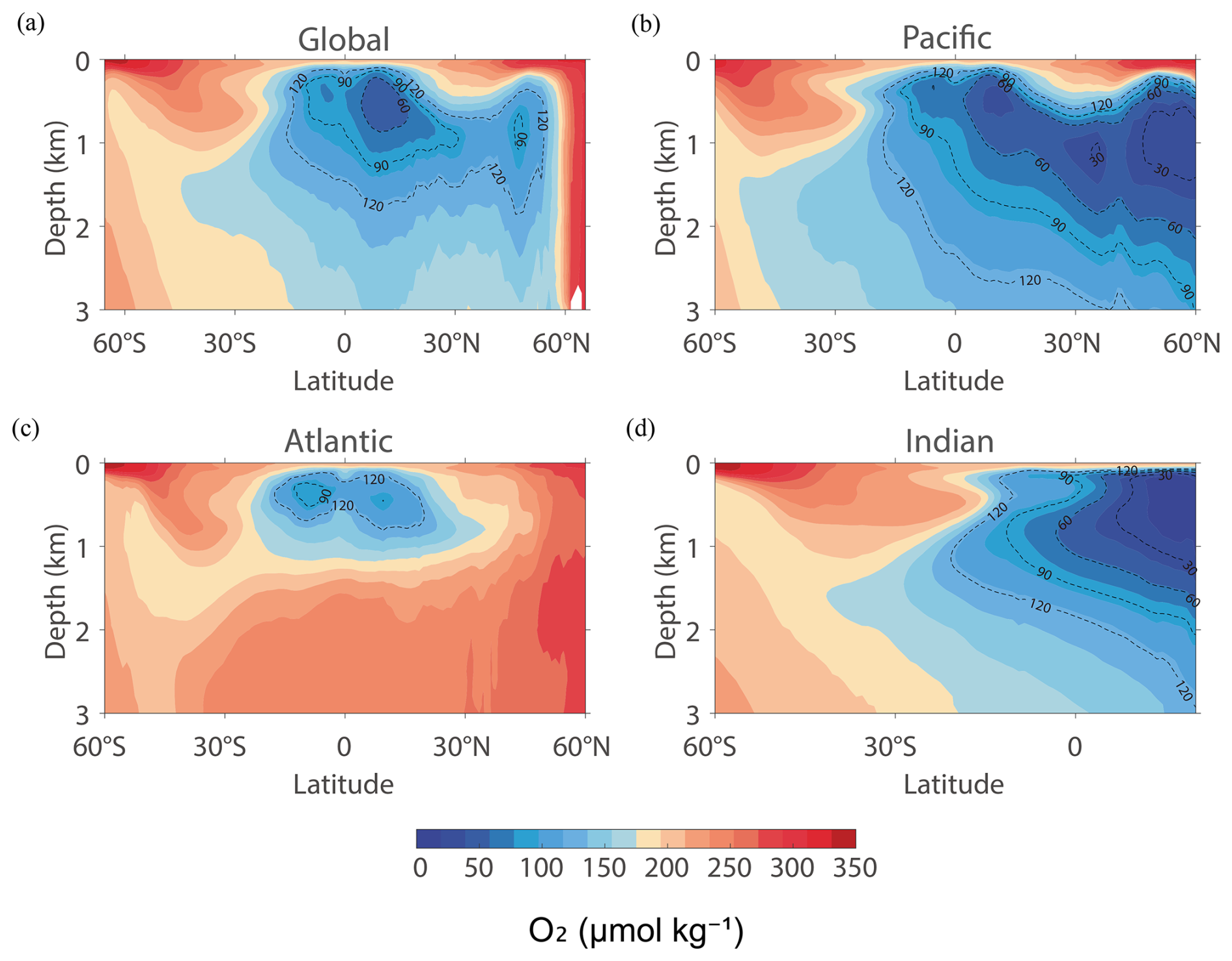
Figure 11 Comparison of zonal mean O₂ climatology (IAP climatology, unit: µmol kg⁻¹) in the (a) Global Ocean, (b) Pacific, (c) Atlantic, and (d) Indian Oceans.

3.5 Oxygen minimum zones

Oxygen minimum zones (OMZ) are important regions that impact marine organism distributions and biogeochemical cycling. OMZ occur in various regions such as the tropical Pacific and Atlantic Oceans, the North Pacific Ocean, and the North Indian Ocean, posing challenges for marine organisms adapted to higher O₂ concentrations (Stramma et al., 2008, 2021). In various studies, OMZ are bounded by different thresholds of O₂ levels. Here, we select two typical thresholds of 60 and 90 µmol kg⁻¹ to define OMZ (Ito et al., 2025), referred to as OMZ60 and OMZ90, respectively.

The zonal mean O₂ of the IAP climatology dataset for global and three major basins are shown in Fig. 11. Globally, the zonal mean OMZ90 regions are mainly located within 200–1200 m and 5° S–30° N, associated with upwelling and high O₂ consumption. The Pacific Ocean contains the largest volume of OMZ60 and OMZ90 among the three ocean basins, with the OMZ90 extending from ∼ 15° S to ∼ 60° N and from a depth of ∼ 200 to ∼ 3000 m. There is a gradual increase in the max depth of OMZ90 and OMZ60 in the Pacific Ocean from ∼ 15° S to ∼ 60° N; thus, the OMZ in the North Pacific Ocean has greater vertical extent. The OMZ in the North Pacific Ocean is also more severe because there is a notable region with zonal O₂ levels less than 30 µmol kg⁻¹ in the ∼ 700 to ∼ 1500 m layer. The OMZ90 in the Indian Ocean extends from ∼ 10° S to the northernmost end and is located from ∼ 20 down to a maximum depth of 1800 m. In the Atlantic Ocean, the OMZ90 is located within a 300–500 m layer, with an area much smaller than that of the Pacific and Indian Oceans (Table 2).

Table 2 The volume of OMZ60 and OMZ90 calculated from the annual mean climatology for each basin and for different products. The values are in the units of 10⁶ km³.

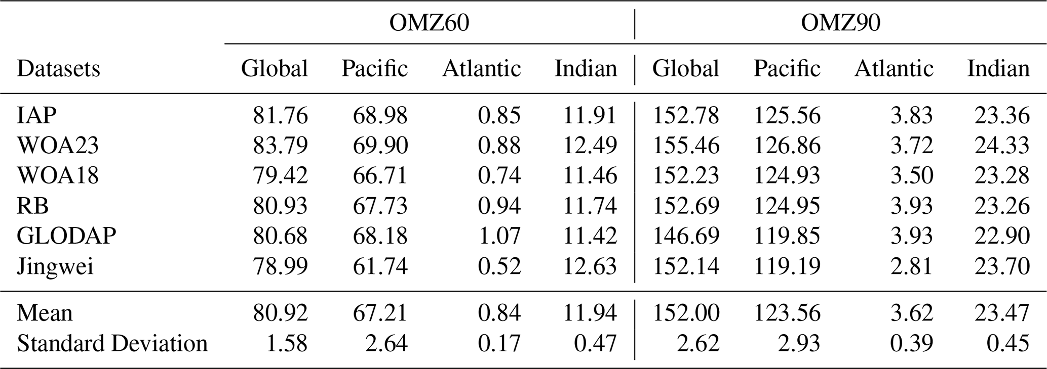
We also calculated the volume of OMZ60 and OMZ90 globally and for each basin in Table 2 using six datasets (excluding GOBAI and SJTU because their maximum depth only reaches about 2000 m below the ocean surface). The global volume of OMZ60 and OMZ90 is generally consistent among the datasets, with a standard deviation of 1.95 % and 1.72 % across the products for OMZ60 and OMZ90, respectively. The Pacific Ocean contains most of the OMZ (83.05 % of the global OMZ60 and 81.29 % of the global OMZ90), with a standard deviation of 3.93 % and 2.37 % across the products. The Atlantic Ocean contains about 1.04 % and 2.38 % of the global OMZ60 and OMZ90, respectively, which is the lowest among the three ocean basins. The standard deviation is 20.24 % and 10.77 % for the Atlantic Ocean OMZ60 and OMZ90, respectively. The estimated OMZ for the Atlantic Ocean may be more sensitive to the horizontal resolution, mapping method, and so on.

The OMZ areas as a function of depth and density are shown in Fig. 12. The density layers are calculated with the Gibbs-SeaWater Oceanographic Toolbox (IOC et al., 2010; McDougall and Barker, 2011; Kwiecinski and Babbin, 2021), using the gridded temperature and salinity climatology products of IAP (Cheng et al., 2024). The maximum OMZ60 area occurs at a depth of ∼ 800 m and a density of 27.75 kg m⁻³ for all the datasets. Most OMZ60s exist in the upper 2000 m. So that all the climatologies including GOBAI and SJTU with the maximum depth of 2000 m could be involved in the analysis of OMZ areas at depth levels. GOBAI and SJTU exhibit a larger OMZ60 volume within the upper 2000 m compared to other products, and the maximum depth of SJTU OMZ60 is ∼ 1700 m, which is shallower than that of the other products. At density levels, the products are very consistent, and SJTU shows a larger area of OMZ60 near the 27.4 kg m⁻³ level and Jingwei shows a smaller area of OMZ60 near the 27 kg m⁻³ level.

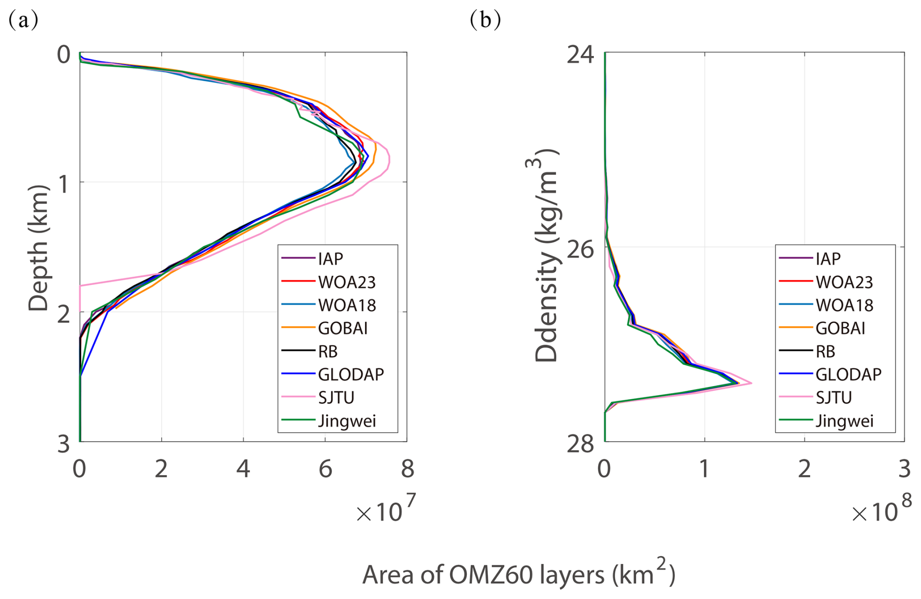
Figure 12 The global horizontal area of OMZ60 in each interpolated layer with respect to depth and (b) density.

Figure 11a–c shows the horizontal OMZ60 area at depth levels for the Pacific, Atlantic, and Indian Oceans, respectively. Consistent with the volume assessment in Table 2, the Pacific Ocean contains the largest OMZ60 area, followed by the Indian and Atlantic Oceans. The maximum OMZ60 area occurs at a depth of about 800 m in the Pacific and Indian Oceans, but at a much shallower depth of ∼ 400 m in the Atlantic Ocean. Jingwei shows the largest difference from the other products in the Pacific and Indian Oceans at the upper 500 m depth. SJTU shows a larger area of OMZ60 in the Pacific and Indian Oceans but a smaller area in the Atlantic Ocean than the other products (Fig. 13). Collectively, different products show a spread of ±4 × 10⁶ km² for the Pacific OMZ60 and of ±1 × 10⁶ km² for the Indian and Atlantic OMZ60 (Fig. 13d–f), except that Jingwei shows a very large difference of up to $-\mathrm{9}\times {\mathrm{10}}^{\mathrm{6}}$ km² at the depth around 500 m for the Pacific OMZ60 area compared to the ensemble mean (Fig. 13d).

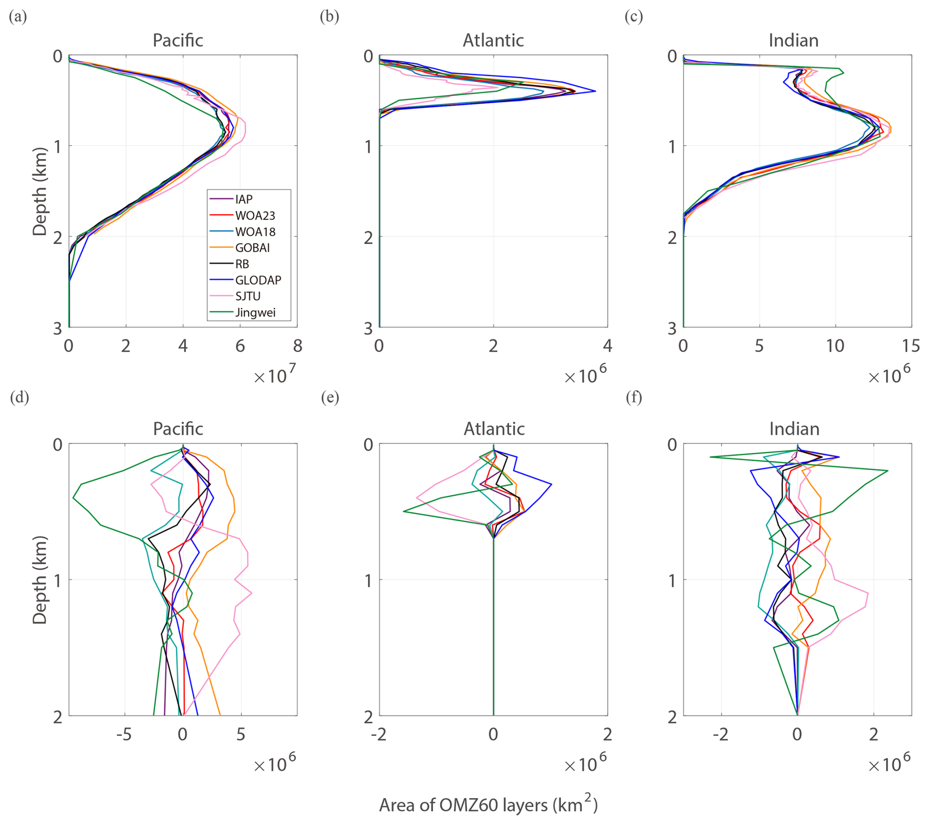
Figure 13 OMZ60 area for the Pacific, Atlantic, and Indian Oceans in units of 10⁶ km². The upper row is the vertical distribution of the OMZ areas: (a) Pacific, (b) Atlantic, (c) Indian. The lower row is the differences in the OMZ areas relative to the ensemble mean: (d) Pacific, (e) Atlantic, (f) Indian.

4 Conclusions

Observationally-based gridded data products provide a basis for detecting and understanding ocean O₂ changes at various spatial and temporal scales. These observational datasets are also used to validate the computational ocean biogeochemistry and earth system models. This study provides a quantitative description of the O₂ climatology, annual cycle, and OMZ distribution with eight O₂ data products. There have been several new O₂ data products developed in recent years, which makes this comparative analysis timely.

The global mean O₂ shows a well-established high-low-high vertical structure and a good consistency among all products. The global mean O₂ concentrations of the products over depth generally agree within ±3 µmol kg⁻¹. Regionally, the gridded mean difference of the 0–1000 m mean O₂ is mainly within ∼ 12 µmol kg⁻¹. For the global 0–100 m O₂ annual cycle, O₂ anomalies (differences from the annual mean) ranges from −1 to 0.8 µmol kg⁻¹, but the inter-products difference (defined by the standard deviation of four datasets that provide a monthly climatology) can be as large as ∼ 0.3 µmol kg⁻¹, indicating a similar signal-to-noise ratio among the four datasets of monthly climatology. We also analyzed the OMZ distribution for different climatology datasets. Different products show a spread of ±4 × 10⁶ km² for the Pacific OMZ60 and ±1 × 10⁶ km² for the Indian and Atlantic OMZ60.

The assessments presented in this study demonstrate the consistency and differences among available products, supporting their future use. Substantial local differences (±25 µmol kg⁻¹ for the upper 1000 m climatological mean) can be seen, which could influence the baseline from which anomalies and trends are calculated and could give an insight into regions that are relatively more sensitive in the process of gridded data reconstruction, such as the subpolar North Pacific, the Southern Ocean fronts, and the eastern Pacific regions close to OMZ boundaries where the spatial O₂ gradient is large.

The overall spread across products results from all uncertainty sources (e.g., measurement errors, mapping errors, different time periods, etc.). Controlled intercomparisons that isolate each uncertainty source are needed in the future to understand the contribution of a single factor, especially in regions showing a large spread. It will eventually help the community to improve the methodologies and reduce the spread in the future. Another caveat is that only a limited number of products are included in this inter-comparison. We hope to maintain and extend this activity in the future and serve as a regular intercomparison exercise to provide critical information to the data users.