The Scotland–Canada overturning array (SCOTIA): twenty years of meridional overturning in the subpolar North Atlantic

The Atlantic meridional overturning circulation (AMOC) is expected to decline dramatically over the 21st century, with severe impacts for Northern Hemisphere climate. After 20 years of sustained monitoring in the subtropics, a detectable AMOC weakening trend is now beginning to emerge. However, continuous observations at subpolar latitudes are currently too short-lived to determine any weakening signal above the large-amplitude interannual variability. Here, we introduce a new subpolar observing configuration, SCOTIA (Scotland–Canada overturning array), combining parts of the existing OSNAP mooring array with scattered CTD and Argo data, to extend the record of subpolar AMOC backward in time to cover the subtropical monitoring period, 2004–2024. SCOTIA facilitates a rigorous comparison of the decadal-scale variability in transports and overturning at subpolar and subtropical latitudes. Our results show subpolar AMOC varies on pentadal to decadal timescales with an amplitude comparable to that observed in the subtropics. Anomalously high overturning during 2016–2020 was driven by increased southward transports in the density classes associated with Labrador Sea Water. We find no statistically significant trend in subpolar AMOC during the period 2004–2024.

1 Introduction

The Atlantic meridional overturning circulation (AMOC) transports warm water northward and is a principal control over ocean heat distribution and climate in the Northern Hemisphere. AMOC decline is among the most consequential impacts of anthropogenic climate change (van Westen and Baatsen, 2025), and has been suggested by theory (Stommel, 1961), paleo proxy records (Caesar et al., 2021), and climate simulations (Weijer et al., 2020). Several paleo records indicate that the AMOC has weakened dramatically during the industrial era (Caesar et al., 2021), while state-of-the-art climate simulations suggest no significant trend during 1850–2014 but project dramatic decline over the course of the 21st century (Weijer et al., 2020). This lack of consensus over past and present AMOC behaviour has called into question the confidence in CMIP model projections (McCarthy and Caesar, 2023).

Systems for directly observing the AMOC have been installed in recent decades. The RAPID array was installed in 2004 to monitor the AMOC strength in the subtropical North Atlantic at ∼26.5° N with 12-hourly temporal resolution. This calculation relies upon measuring the transatlantic thermal wind shear using hydrographic moorings at the eastern and western boundaries, with velocities in boundary currents and the Florida Current observed directly (McCarthy et al., 2015). The overturning at RAPID is typically presented in depth space, although a recent analysis by Smeed et al. (2026) presents the overturning at RAPID in density coordinates. In spite of a sudden step-down in AMOC strength observed in 2009, the RAPID time series has generally been considered too short to resolve any anthropogenic AMOC weakening signal over the noise of stochastic interannual variability. However, recent analysis suggests that, after 20 years of sustained observing, a statistically significant weakening trend of $\sim -\mathrm{1}$ Sv per decade is now detectable in the RAPID time series (McCarthy et al., 2025).

Since 2014, the Overturning in the Subpolar North Atlantic (OSNAP) array has provided a record of the AMOC strength at subpolar latitudes (Lozier et al., 2019), complementing the subtropical observations on the RAPID array. The OSNAP array consists of two subarrays: OSNAP west, which connects the east coast of Canada with southwest Greenland; and OSNAP east which stretches from southeast Greenland to Scotland. This configuration allows subpolar overturning to be partitioned into contributions from processes occurring east and west of Greenland (e.g. Lozier et al., 2019; Li et al., 2021; Fu et al., 2023a, 2025), and captures the volume transports of both freshwater and dense overflow water by the Greenland boundary currents (e.g. Pacini et al., 2020; Foukal and Pickart, 2023; Koman et al., 2024; Sun et al., 2025). The AMOC calculation at OSNAP is again reliant on thermal wind shear across interior ocean basins computed from hydrographic moorings located either side. However, because the AMOC at OSNAP is computed in density coordinates, it is sensitive to these basins' interior density structure. Furthermore, the OSNAP section crosses a region with more complex topography than at RAPID, so relies more heavily on direct velocity observations in several narrow, barotropic boundary currents. As a result, the OSNAP array is highly resource intensive, currently comprising around 50 hydrographic moorings compared to just 9 at RAPID.

The AMOC observed by the OSNAP array exhibits no significant trend, potentially because this 10 year record remains too short to resolve any anthropogenic climate signal. Although first installed in 2014, some components of the OSNAP array have been in place longer. Specifically, the western boundary current has been observed by the 53° N mooring array since the mid 1990s, while regular Ellett Array hydrographic sections across the North Atlantic Current pathway have been operating since the mid 1970s, meaning that at least some data from the westernmost and easternmost boundaries are available from before 2014. The advent of the Argo programme in the early 2000s means that the hydrography of the Atlantic interior is also well observed before 2014. These longer-term observations introduce the potential for calculating subpolar overturning strength over a longer time period, facilitating a rigorous comparison of decadal-scale variability at the subpolar latitudes with observed changes in subtropical latitudes.

In this paper, we generate a 20 year observational record of the AMOC on a new transatlantic section, the Scotland–Canada overturning array (SCOTIA, Fig. 1). This section coincides with the OSNAP line at the western and eastern boundaries but crosses the subpolar North Atlantic directly without intersecting Greenland. Combining available mooring, Argo and CTD profiles, we generate gridded temperature and salinity fields across the subpolar North Atlantic from 2004–2024 with monthly temporal resolution. These data are then combined with satellite altimetry and atmospheric reanalysis to generate the corresponding velocity field on the section, from which we diagnose the AMOC in density coordinates. We validate this time series by comparison with the equivalent calculation on the OSNAP line since 2014 then, extending back to 2004, compare the 20 year subpolar AMOC record with results from the subtropical RAPID array.

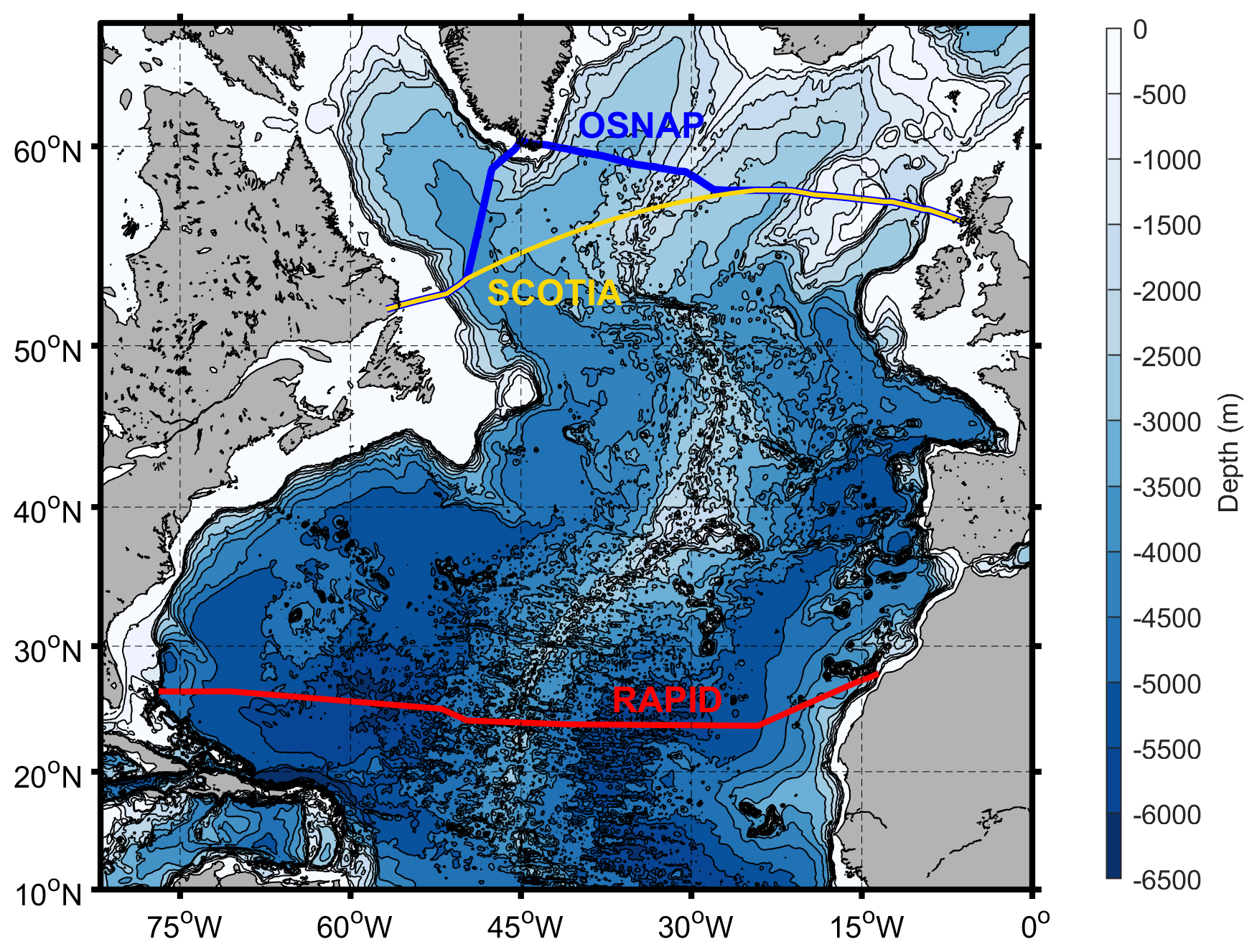
Figure 1 Bathymetric map of the North Atlantic showing the locations of the RAPID (2004–present), OSNAP (2014–present), and SCOTIA (2004–present) sections.

2 Methods

2.1 The SCOTIA line

The SCOTIA line follows the OSNAP line at the western and eastern boundaries but crosses the subpolar North Atlantic directly without intersecting Greenland. SCOTIA connects the 53° N mooring array in the Labrador Sea in the west with Iceland Basin and Rockall Trough Ellett Array mooring arrays in the east, with the central section following a great circle path. Full coordinates for the SCOTIA line are included in the associated data files.

Across deep basins – areas where flow is overwhelmingly geostrophic and without complex topography – the vertical shear in transports normal to a section is entirely defined by the vertical structure of pressure at the boundaries. This can be measured with dynamic-height moorings at each side of the basin. The determination of net transport then requires a basin-wide velocity or pressure gradient reference to set the amplitude of the barotropic part of the flow. The horizontal spatial distribution of this barotropic flow across deep basins is largely irrelevant to the depth-space overturning calculation (Johns et al., 2005; McCarthy et al., 2015). These ideas are so powerful that basin-wide overturning estimates, particularly those calculated in depth space, largely do not attempt to observe the time-varying barotropic velocities away from the boundaries over the ocean interior, instead relying on a compensation transport to reproduce their effect on overturning.

For a density-space overturning calculation, as required in subpolar latitudes, things are slightly more complicated as the horizontal distribution of compensation velocities can impact the estimate of overturning via horizontal variability in the depth of maximum overturning. OSNAP tackles this using detailed current observations from moored current meters near strong topography while relying on the end-point analysis and compensation transports across basin interiors.

Now consider the SCOTIA section. Examination of output from the Viking20x model (Biastoch et al., 2021; Getzlaff and Schwarzkopf, 2024), a high-resolution ocean model hindcast, suggests that the end-point analysis described above is inadequate to estimate the density-space overturning across the long interior section. This is due to the combination of the topography across the mid-Atlantic ridge and strong horizontal density gradients. Instead, to reliably observe overturning and transports across the SCOTIA interior section requires fully-determined, referenced, geostrophic currents (in the horizontal, vertical and in time) (Fig. S3). For this, first we require monthly temperature and salinity across the whole SCOTIA section gridded in the horizontal and vertical.

2.2 Generating monthly gridded temperature and salinity fields

Monthly temperature and salinity fields are constructed along the entire length of the SCOTIA line. Our approach is built around isolating the anomalies of in situ observations relative to the mean and seasonal cycle, which is well resolved by observations. These anomalies are then linearly interpolated in 3D ($x,z,t$) onto the SCOTIA grid, and the mean and seasonal cycle is then added back in. This means the final fields remain faithful to in situ observations while retaining a rich and realistic spatial and temporal structure.

The grid has a nominal horizontal resolution of 15 km across the central Great Circle section, with 3 km resolution in the west and east, a vertical resolution of 20 m, and monthly temporal resolution. Horizontal grid spacing is adjusted to ensure that grid nodes coincide with the average mooring locations.

2.2.1 Monthly mean climatology

We construct a monthly mean seasonal climatology for SCOTIA temperature and salinity fields following the methods of Curry (1996) and Jones et al. (2023). This climatology utilises all available mooring, Argo and CTD profile data. These profiles are averaged in depth space within the mixed layer, and on isopycnals below the mixed layer to preserve vertical structure in the presence of isopycnal heave.

Observations up to 100 km from the SCOTIA line (60 km on the European continental shelf) and between 2004–2025 are included in the product (Figs. 2b and S1a in the Supplement). A centre-weighted variable search radius, dependent on data density, is used to populate the grid cells. CTD profiles with poor vertical resolution (<15 observations), and those sampling only part of the water column were excluded. Mooring data are averaged into month-mean profiles prior to gridding, to prevent their higher sample rate biasing the mean. The region covered by the 53° N mooring array has excellent data coverage, so the search radius is fixed at 2 km to preserve the strong horizontal density gradients in this region. A partition was manually imposed at −34° E to prevent data from being “smeared” across the mid-Atlantic ridge.

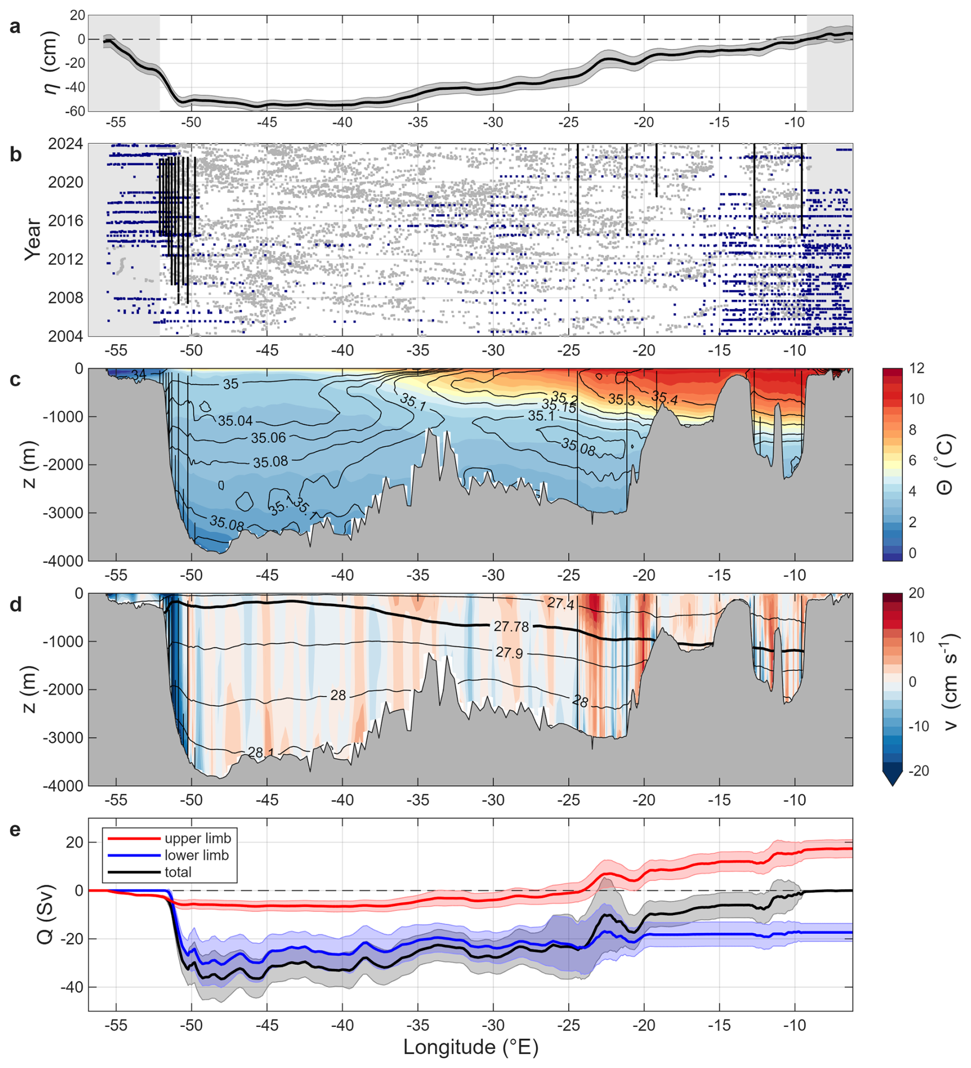
Figure 2 Constructing density-space transports from gridded satellite altimetry and scattered hydrographic profiles. Panel (a) shows the 2004–2024 mean and standard deviation of the satellite-derived absolute dynamic topography along the SCOTIA section, while panel (b) shows the spatiotemporal distribution of CTD (blue) and mooring (black) and Argo (grey) profiles along the section. Greyed-out regions in panels (a) and (b) indicate where GLORYS reanalysis has been used in place of direct observations on the Scottish and Canadian shelves. Panel (c) shows the time-mean gridded conservative temperature (Θ, colour scale) and absolute salinity (S [g kg⁻¹], contour lines) fields on the SCOTIA section, with moorings denoted as vertical black lines. Panel (d) shows the corresponding neutral density (γ [kg m⁻³]) field with time-mean γ_MOC highlighted in bold, alongside the time-mean section-normal velocity field (colour scale) computed from thermal wind shear referenced to absolute dynamic topography (panel a). Panel (e) shows the mean and standard deviation of the transport accumulated from west to east for the upper limb (γ<γ_MOC), the lower limb (γ>γ_MOC), and the total (cf. Fig. 2 of Lozier et al., 2019).

2.2.2 Vertical interpolation and extrapolation of mooring data

Data from the Ellett Array are linearly interpolated onto the 20 m vertical grid following Fraser et al. (2022). For the 53° N mooring data, vertical interpolation is performed using a CTD and Argo-derived local gradient method (Johns et al., 2005) to resolve the complex halocline structure (note that AMOC estimates are particularly sensitive to the vertical interpolation method employed for the 53° N mooring array). For all moorings across the SCOTIA line, near-surface temperature is interpolated between the topmost instrument and the satellite SST value using Argo-derived climatological vertical gradients. The corresponding salinity is populated using the topmost instrument and the climatological gradient only.

2.2.3 Extending Argo temperature and salinity to the seabed

Most Argo floats profile to 2000 m, so the deep ocean is comparatively data sparse. The main symptom of this abrupt reduction in data density is an unphysical step in climatological profiles at 2000 m. A separate sub-2000 m climatology is therefore constructed with parameters tuned to optimise the available deep data. As there is no resolvable seasonal cycle below 2000 m, we use all available CTD profiles to construct a mean section. Large horizontal data gaps in the sub-2000 m domain are filled using linear horizontal interpolation.

Argo profile data are appended below 2000 m using this deep climatology. To prevent a vertical step in the composite profile, an offset is applied to the top of the sub-2000 m data, diminishing linearly to zero at 2750 m. The profile is then incorporated into the isopycnal averaging scheme used to construct the monthly mean climatology.

2.2.4 Time-varying gridded temperature and salinity fields

Anomalies of in situ CTD, mooring and Argo profiles are computed relative to the monthly mean climatology. These anomalies were then translated onto the SCOTIA grid using a 3D linear interpolation across distance (x), depth (z) and time (t). Note that since the profile data are dense in z but comparatively sparse in x and t, this is conceptually similar to a 2D (x,t) interpolation on each depth level. Deeper than 2000 m, where data are especially sparse, CTD and Argo-derived anomalies are linearly tapered to zero at 2750 m, to prevent the unphysical propagation of anomalies across large intervals of distance and time. The mean and seasonal cycle, from the monthly mean climatology, is added to the gridded anomalies to produce the monthly temperature and salinity fields. The fields are corrected for any unstable stratification using the Gibbs SeaWater (GSW) Oceanographic Toolbox of TEOS–10 (McDougall and Barker, 2011). Finally, due to data sparsity on the Scottish and Canadian shelves, we follow the methodology of OSNAP in using output from the Global Ocean Physics Reanalysis (GLORYS12V1, hereafter “GLORYS”, Lellouche et al., 2021) for the temperature and salinity fields on the Scottish and Canadian shelves.

From these final temperature and salinity fields, we compute the corresponding neutral density field (Jackett and McDougall, 1997). The resulting mean SCOTIA sections for conservative temperature (Θ), absolute salinity (S) and neutral density (γ) are shown in Fig. 2c and d.

2.3 Velocity component normal to the section

To fully determine our geostrophic velocity fields from observations we use thermal wind calculations from the monthly SCOTIA temperature and salinity fields referenced to monthly mean satellite absolute dynamic topography (ADT; Copernicus Marine Service, 2025). Geostrophic currents were calculated using the Python Gibbs SeaWater (GSW) Oceanographic Toolbox of TEOS–10 (McDougall and Barker, 2011). To these were added Ekman surface transports derived from ERA5 wind stress data (Hersbach et al., 2020, 2023). Ekman surface currents were calculated by splitting the transport evenly across the top 60 m of the water column. The results were not sensitive to the details of the Ekman velocity profile. As with the temperature and salinity fields, we use velocity fields from GLORYS on the Scottish and Canadian shelves.

We tested other velocity calculation methods, following OSNAP and RAPID methodology in using direct moored current meter data when available in the western boundary and Rockall Trough, regions of strong currents and steep topography. This gave no qualitative advantage over the use of geostrophy across the full section, while introducing a step-change in the methodology corresponding to the deployment of moored current meters on the Ellett Array halfway through the 20 year time series. Further details of the alternative data and velocity calculations can be found in the Supplement (SI, Sect. S4).

2.3.1 Compensation velocities

Compensation transports, applied as a constraint on the net mass (or volume) flux are an essential tool in overturning observation, primarily used to represent unmeasured, mostly barotropic, flows but also to compensate for measurement uncertainty. On short timescales, such compensation transports can be tens of Sverdrups, larger than the overturning transport signal being sought, though generally substantially smaller than the gross poleward or equator-ward transport. This compensation is usually applied via spatially uniform velocities over some subsection of the full array. It is common practice (OSNAP, RAPID) to locate the compensation in regions where current shears are calculated from the density structure using thermal wind. This is analogous to choosing a reference level for the geostrophic velocity calculation, and the use of such compensation velocities is an important component of overturning observation.

For the SCOTIA section, we attempt to fully determine the geostrophic flows from the gridded monthly temperature and salinity fields referenced to monthly satellite ADT at the surface. However, compensation velocities are still required to balance the flow.

The long interior section with no continuous mooring data, between about 50° W (mooring K10) and 24° W (mooring IB3) contains the mid-Atlantic ridge, which is capable of supporting horizontal pressure gradients. The presence of this ridge emphasises accurate determination of density on its flanks below the top of the ridge (about 1500 m). However, with no deep moorings on the flanks of the ridge and Argo data generally stopping at 2000 m, deep temperature and salinity data are sparse and so their structure and variability are more uncertain, this potentially introduces errors and mean biases into the overturning calculations. A second potential source of transport imbalance is mismatches in spatial resolution between ADT, density structure, and bathymetry. Finally, ageostrophic, non-surface-Ekman flows will not be observed by the methods described here. Analysis of likely extent and amplitude of these possible errors in the Viking20x model output suggests possible systematic bias towards overestimating mean southward flow by 5–10 Sv at depth. Importantly, little bias was found in the upper limb transport due to any of these factors.

All the mechanisms identified here as possible sources of systematic errors or biases in our transport calculations – below 2000 m and the westernmost part of the section – are dominated by lower limb waters. Combining these arguments with the comparison of transport in depth and density space between SCOTIA and OSNAP (Fig. S2a and b) suggests a two-part compensation strategy. The mean transport imbalance is compensated below 1800 m, with the adjustment increasing linearly between 1800–4000 m. In contrast, the time-varying transport imbalance is addressed using the conventional approach of applying a spatially uniform compensation velocity across all depths. In this way the mean compensation has no impact on the estimate of MOC (though it will marginally impact mean temperature, salinity and density fluxes). The time-varying part of the compensation transport and its contribution to the MOC time series is seen in Fig. S2c and d.

2.4 Overturning metrics

We compare overturning and transports at SCOTIA, OSNAP and RAPID using five key metrics: the traditional four – the maximum of the overturning streamfunction (MOC), the density at which this maximum occurs (γ_MOC), northward heat transport (ℋ), northward freshwater transport (ℱ) – and, more unusually, the density flux (𝒟).

The first four of these are entirely consistent with previous literature, perhaps beyond mentioning that freshwater transports use a section-average salinity reference and that we adopt the neutral density variable. However, we will briefly introduce the density flux, 𝒟. For full details see Fox et al. (2025).

2.4.1 Density flux

The zonally integrated overturning streamfunction in density space, Ψ(γ,t), can be written:

$$\begin{array}{}\text{(1)}& {\displaystyle }{\displaystyle }\mathrm{\Psi }\left(\mathit{\gamma },t\right)=\underset{R\left(\mathit{\gamma },t\right)}{\iint }v\left(x,z,t\right)\mathrm{d}z\mathrm{d}x,\end{array}$$

where R(γ,t) is the part of the (x,z) vertical plane defined by ${\mathit{\gamma }}_{\text{min}}<{\mathit{\gamma }}^{\prime }\left(x,z,t\right)<\mathit{\gamma }$, that is, we integrate over the area with neutral density less than γ. Here $x\in [w,e]$ is the along-section coordinate, $z\in [-H,\mathit{\eta }]$ is the vertical coordinate (positive upwards), and $v\left(x,z,t\right)$ is the velocity normal to the section. H(x) is the water depth and η(x,t) the sea surface height. We then define, in the usual way, the meridional overturning, MOC_γ(t), as the maximum of Ψ for all γ, and γ_MOC(t) as the density at which this maximum occurs:

$$\begin{array}{}\text{(2)}& {\displaystyle }& {\displaystyle }{\text{MOC}}_{\mathit{\gamma }}\left(t\right)=\underset{\mathit{\gamma }}{max}\left[\mathrm{\Psi }(\mathit{\gamma },t)\right]\text{(3)}& {\displaystyle }& {\displaystyle }{\mathit{\gamma }}_{\text{MOC}}\left(t\right)={\text{arg\hspace{0.17em}max}}_{\mathit{\gamma }}\left[\mathrm{\Psi }(\mathit{\gamma },t)\right].\end{array}$$

The northward meridional density flux (𝒟):

$$\begin{array}{}\text{(4)}& {\displaystyle }{\displaystyle }\mathcal{D}\left(t\right)=-\underset{{\mathit{\gamma }}_{\text{min}}}{\overset{{\mathit{\gamma }}_{\text{max}}}{\int }}\mathrm{\Psi }\mathrm{d}\mathit{\gamma },\end{array}$$

the area under the streamfunction curve. We follow convention in referring to this as “density flux” while the units of kg s⁻¹ perhaps suggest “mass flux”. However, the term “density flux” captures the process intuitively – with lighter water flowing northwards and denser water returning southward being characterised as a southward (or negative northward) density flux. We can see this more clearly by rearranging Eq. (4) for the case of no net throughflow (which is true by construction for the observational sections studied here), it is straightforward to show that

$$\begin{array}{}\text{(5)}& {\displaystyle }{\displaystyle }\mathcal{D}=\underset{w}{\overset{e}{\int }}\underset{-H}{\overset{\mathit{\eta }}{\int }}v\mathit{\gamma }\mathrm{d}z\mathrm{d}x,\end{array}$$

the northward flux of density γ by velocity v.

The advantages of including density flux in our suite of overturning metrics, and possible problems associated with relying too heavily on MOC_γ, have been demonstrated on seasonal timescales (Fox et al., 2025), however it isn't yet clear how this applies at longer time-scales.

More than other commonly used overturning metrics, density flux helps describe changes in the most relevant physical property for ocean dynamics – density. It also explicitly retains the link between overturning observation and the powerful watermass transformation theory (Tziperman, 1986; Speer and Tziperman, 1992; Nurser et al., 1999). Density flux forms part of the mass balance in the ocean (under the Boussinesq approximation): density fluxes across lateral boundaries into a region are balanced by surface density fluxes integrated over the whole region and changes in total mass, this balance is unaffected by interior mixing. MOC_γ, by contrast, is part of the volume balance of the upper (or lower) limb, balanced by interface heave and transformation across the interface. These transformations are primarily driven surface fluxes where the interface outcrops and internal mixing across the interface. Considering both density flux and MOC_γ, which are easily calculated from the same observations, gives a more complete and balanced description of overturning.

3 Comparing SCOTIA with OSNAP

We first compare overturning and transports on the SCOTIA line with those on the established OSNAP line. We note that we do not expect a strict one-to-one correspondence between parameters on the two lines. Differences will exist due to surface forcing, internal mixing and internal storage in the triangular region, mostly in the Irminger Basin, lying between the OSNAP and SCOTIA lines (Fig. 1). Nonetheless, we expect a high-degree of correspondence between the overturning at SCOTIA and OSNAP, so this comparison is useful as a first-order validation. For consistency with the OSNAP data product, we translate our analysis from neutral density (γ) coordinates to potential density (σ₀) coordinates for this portion of the analysis.

To assess how the difference in location impacts overturning and transport metrics on the SCOTIA and OSNAP lines, we again turn to output from the Viking20x model. Comparing the modelled SCOTIA and OSNAP sections (Fig. S4), MOC, σ_MOC, and density flux show very similar results for the two sections. Overturning and southward density fluxes are generally slightly greater at SCOTIA than OSNAP, the result of surface forcing and watermass transformation in the region between the sections. The density of maximum overturning, σ_MOC, is also found to be consistently slightly greater at SCOTIA that OSNAP. Overall, though, the modelled overturning and transports at the two sections are strikingly similar, supporting our use of OSNAP as ground truth for our new section.

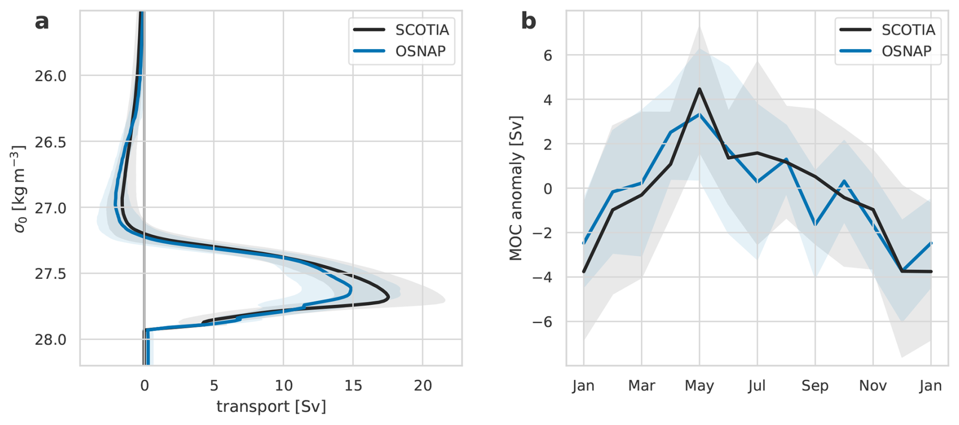
Figure 3 (a) Mean overturning streamfunctions [Sv] in density space for SCOTIA (black line) and OSNAP (blue line). Shaded areas show the standard deviation of the streamfunction. (b) The seasonal cycle of overturning anomalies for SCOTIA (black line) and OSNAP (blue line). Lines show the mean anomaly for each calendar month, shaded areas the standard deviation. The means and seasonal cycle have been calculated for the period spanned by the available OSNAP data (2014–2022), but the SCOTIA results are not qualitatively different when considering the full period (2004–2024).

So we proceed to ground truth our new SCOTIA time series against the established OSNAP time series for the OSNAP period 2014–2022. The SCOTIA mean overturning streamfunction (Fig. 3a) shows about 2 Sv stronger MOC (the maximum of the overturning streamfunction) than OSNAP, with the maximum at a slightly higher density. Both these features are as expected from the model, though with perhaps larger difference between SCOTIA and OSNAP than predicted. Note that to some extent the SCOTIA mean streamfunction has been “tuned” to be close to the OSNAP streamfunction by the choice of spatial distribution of compensation velocity and the use of GLORYS data on the shelves.

We see good agreement in the timing and amplitude of the AMOC seasonal cycle between SCOTIA and OSNAP (Fig. 3b). Fox et al. (2025) find that AMOC seasonality at OSNAP is dominated by a combination of wind-driven surface Ekman transports and the density of the upper ∼500 m at the western boundary. The good agreement between SCOTIA and OSNAP is unsurprising, as seasonal variability of wind fields occurs on horizontal scales which are large compared to the separation of OSNAP and SCOTIA lines, and the two analyses are informed by the same data in the western boundary region.

The time series of SCOTIA MOC is remarkably similar to that for OSNAP (Fig. 4a, correlation r=0.660), generally lying within the OSNAP MOC error bars. Neither time series shows a significant trend over the 2014–2022 period, while the SCOTIA MOC shows slightly higher variance. Indeed, SCOTIA displays larger variability than OSNAP on most time scales (Fig. S6). There are two short periods during which there appears to be a more persistent difference between SCOTIA and OSNAP MOC, in summer/autumn 2016 and 2019. In both cases SCOTIA suggests more overturning than recorded at OSNAP. Corresponding differences between SCOTIA and OSNAP are seen in the density, heat and freshwater fluxes (Fig. 4c–e) in 2019, though less so in 2016. In 2019 the observed differences in heat and freshwater flux between SCOTIA and OSNAP act in opposite directions, possibly suggestive of warming and salinification of the upper ocean waters in the region between the two sections, with the warming dominating. We have not been able to definitively pin these differences down to either a real physical effect or a result of the different observations and methodologies employed by the two analyses.

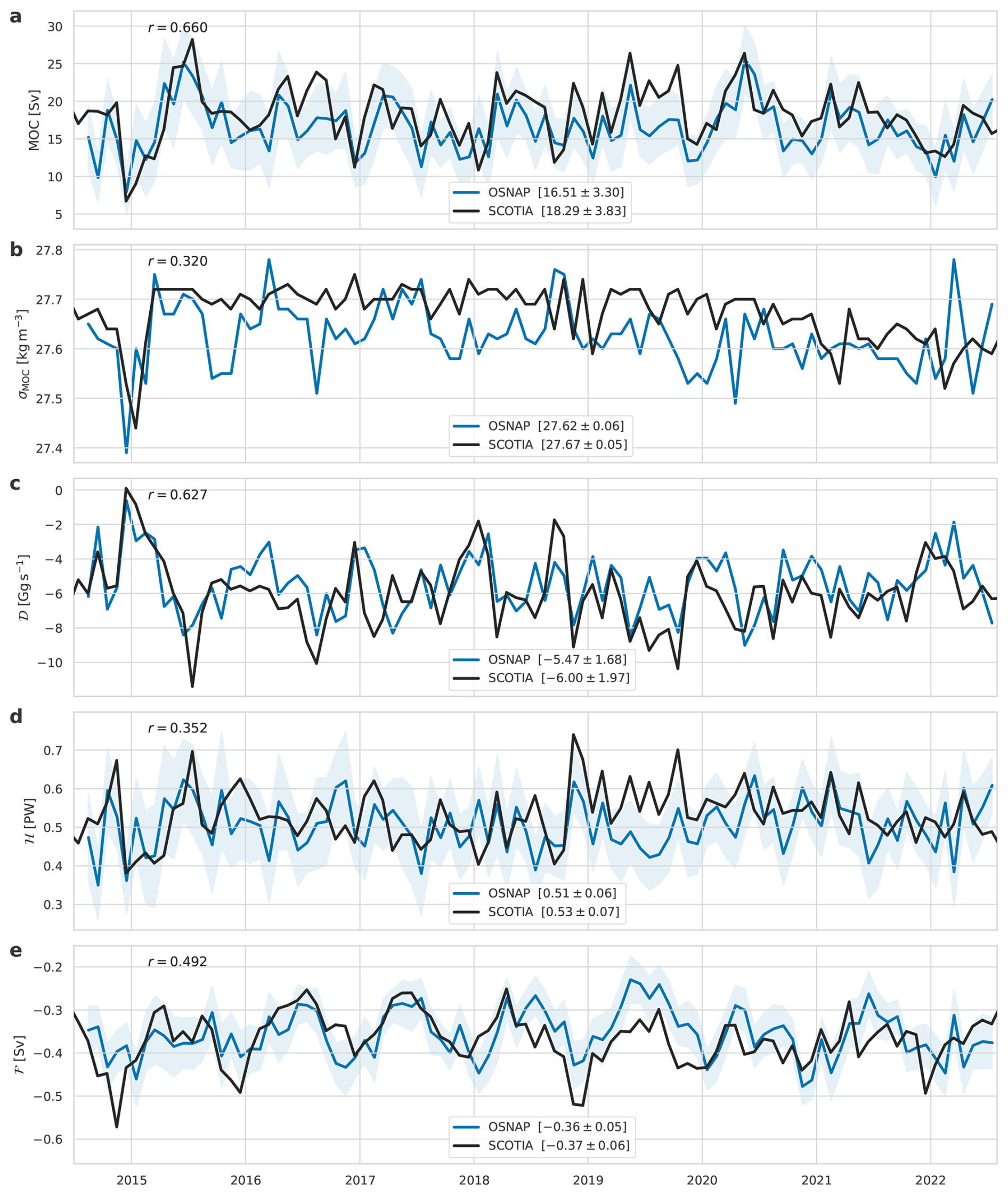
Figure 4 Time series of (a) MOC, (b) σ_MOC, (c) northward density flux 𝒟, (d) northward heat flux ℋ, and (e) northward freshwater flux ℱ from SCOTIA (black) and OSNAP (blue) for the period covered by the available OSNAP data (2014–2022). The mean and standard deviation of each time series are shown in square brackets. Correlation coefficients r are all significant at the 95 % confidence level. Blue shading represents the uncertainties provided with the OSNAP data product.

We now consider the density of maximum overturning (Fig. 4b), which has a correlation of r=0.320 between SCOTIA and OSNAP. This lower correlation perhaps reflects that, on shorter timescales, σ_MOC is very sensitive to local fluctuations in the velocity field. On longer timescales, however, we see many similarities between the two. Both have a large negative anomaly in σ_MOC in winter 2014/15, a time of anomalously low overturning. Both show a long-term shift in σ_MOC towards lower values from 2020 compared to the period 2015–2018. The σ_MOC for SCOTIA appears significantly less “spiky” than OSNAP, possibly because the SCOTIA line lies entirely south of the deep convection sites around Greenland.

Density flux (Fig. 4c) time series, very similarly to MOC, show high correlation (r=0.627) slightly higher variability at SCOTIA, no significant trend and the summer/autumn 2019 higher MOC at SCOTIA is reproduced as more negative northward density flux (i.e. more southward density flux).

Heat fluxes (Fig. 4d) show a smaller correlation between SCOTIA and OSNAP (r=0.352). The only notable shared feature is the low northward heat flux in winter 2014/15 followed by a peak in summer 2015, and again there is an increased northward heat flux in the SCOTIA time series in 2019 which is not seen at OSNAP. Apart from this, the two series both show similar amplitude but unrelated small variability around a value of 0.5 PW. Lagged auto- and cross-correlations performed on these two series (not shown) suggest that both are indistinguishable from a slight seasonal cycle superimposed with white noise.

Freshwater fluxes (Fig. 4e) at both SCOTIA and OSNAP show a marked seasonal cycle (which is also seen reflected, though less clearly, in both MOC and density flux). This seasonal cycle is responsible for the recorded correlation between the two series (r=0.492), and when removed the remaining signals again appear to be “noise” as for heat flux. The seasonal cycle at OSNAP has been examined in detail previously (Fox et al., 2025), and it is no surprise that the cycle at SCOTIA is very similar since the dominant processes are located near-surface in the Labrador Current outflow where the two lines, and the data used in the two calculations, coincide.

Finally, we note that the comparisons in this section have been conducted over a period when OSNAP mooring data is available. SCOTIA uses these mooring temperature and salinity data when calculating anomalies in the west and east of the section. However, when extending the time series back in time to 2004 such mooring-based data are generally not available. To test the possible effects of this reduced data and the possible discontinuity in data availability before and after the start of OSNAP on our estimates, we test the quality of SCOTIA overturning estimates without using any OSNAP mooring-based temperature and salinity anomaly data. We find significant skill in reproducing OSNAP results is still demonstrated by these estimates, though correlations with OSNAP are slightly reduced compared to our “best” estimate (Fig. S5). In particular it is reassuring to note that the exclusion of these data does not change the mean values of the overturning metrics significantly, does not introduce trends in the observed time series and appears to retain the longer term signals including the observed decline in σ_MOC after 2020 and the mismatch between OSNAP and SCOTIA values in 2019. For more details see Sect. S4.

4 A twenty-year record of subpolar North Atlantic overturning

4.1 Comparing SCOTIA with RAPID

Comparison of SCOTIA overturning metrics with those of the established OSNAP line shows that our innovative SCOTIA calculations are performing well. This convinces us that SCOTIA allows, for the first time, presentation of a 20 year, observation-based, monthly time series of overturning in the subpolar North Atlantic. We now revert to neutral density, γ, coordinates (Jackett and McDougall, 1997) as these allow comparison in density space across the wider range of latitudes and depths required to compare subtropical and subpolar density-space overturning.

Examining the new 20 year time series of MOC at SCOTIA, and comparing to the simultaneous RAPID time series (Fig. 5a and b) shows the SCOTIA signal to contain generally higher variability than the RAPID signal at timescales from monthly up to periods of 4–5 years. Both time series show seasonal variations but with different phases, the seasonal maximum at RAPID being later in the year than at SCOTIA, consistent with published results for OSNAP and RAPID sections (Fu et al., 2023a; Fox et al., 2025; Kanzow et al., 2010). There is no obvious correspondence visible between MOC variability at SCOTIA and at RAPID at periods longer than seasonal and up to 4–5 years. Comparing power spectra of MOC at SCOTIA and RAPID (Fig. S7) confirms the generally higher variability at SCOTIA, including a stronger seasonal cycle (peak at 1 year) and, particularly, the stronger variability at a period of 3–4 years. Over the longest timescales observed, while RAPID shows a slow, but significant, decline in MOC of 0.93 Sv decade⁻¹ (95 % CI $[-\mathrm{1.64},-\mathrm{0.22}]$), SCOTIA shows no significant long-term trend (0.42 Sv decade⁻¹, 95 % CI $[-\mathrm{0.39},\mathrm{1.22}]$) in subpolar MOC over the 20 years.

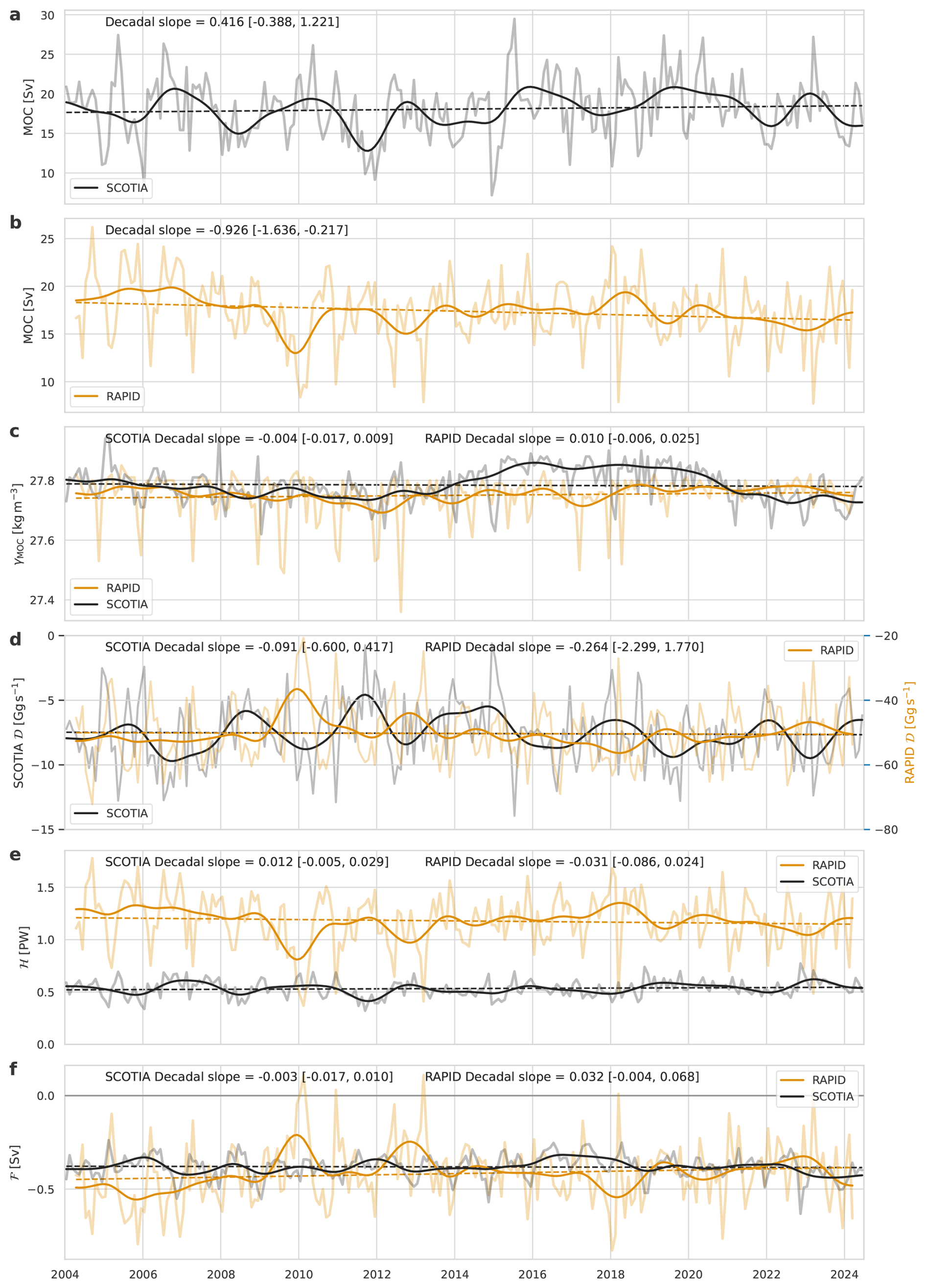
Figure 5 Time series of overturning and transports from SCOTIA and RAPID for the period 2004–2024). Black lines – SCOTIA, amber lines – RAPID. In each case the paler solid lines are the monthly values, darker solid lines the 18 month low-pass filtered time series, and the dashed lines show the trend. The trend and the 95 % confidence limits on the trend (in square brackets) are given in each panel. Panel (a) SCOTIA MOC, (b) RAPID MOC, (c) γ_MOC, (d) northward density flux 𝒟, (e) northward heat flux ℋ, and (f) northward freshwater flux ℱ. In panel (d) the density fluxes have been scaled for easier comparison.

Mean MOC and γ_MOC at SCOTIA closely match those at RAPID (the maxima in Fig. 6). However, the mean overturning streamfunction comparison highlights how overturning at RAPID (Smeed et al., 2026) is associated with much higher southward density flux (the area under the curves in Fig. 6) than at SCOTIA. In the mean, density flux is largely balanced by surface density exchange north of the section, so the area between the two sections represents surface density input (predominantly by cooling) in the region between RAPID and SCOTIA.

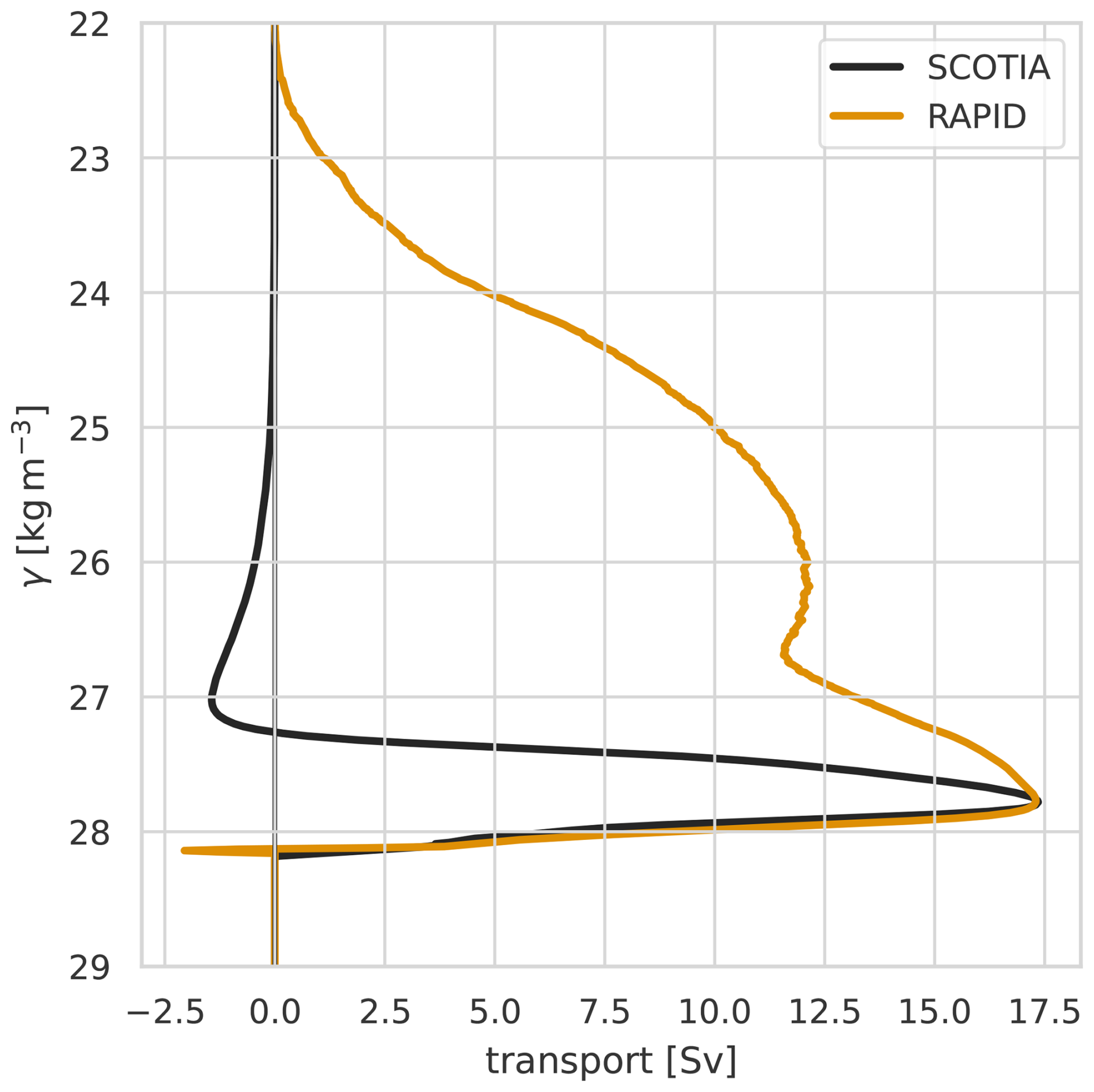
Figure 6 Twenty-year mean overturning streamfunction in density space for SCOTIA (black line) and RAPID (amber line).

Perhaps the most striking feature in Fig. 5 is the increased density of maximum overturning, γ_MOC, at SCOTIA between 2015–2020 (Fig. 5c). We commented on this in the comparison between OSNAP and SCOTIA, where over the OSNAP period it appears in both time-series as a decline in γ_MOC. We now see this event in a wider context as a period of higher γ_MOC between two periods of lower observed γ_MOC.

Turning to the southward density fluxes, 𝒟, in Fig. 5d, these have been scaled to visually match the amplitudes of MOC. The correspondence between the two metrics is remarkably close, suggesting a simple linear relationship between MOC and 𝒟 at timescales longer than seasonal, in both the subpolar (SCOTIA) and subtropical (RAPID) regions. Notably, the observed small downward trend in MOC at RAPID is not seen in the density flux 𝒟. The observed slight weakening of overturning has been counterbalanced by a slight increase in mean density difference between upper and lower limbs. The heat and freshwater fluxes suggest this is most likely due to a slight downward trend in net southward freshwater flux at RAPID rather than changing heat flux.

Tooth et al. (2023) showed how the RAPID overturning streamfunction in density space could be considered a combination of subtropical gyre circulation – giving the secondary peak at around 26 kg m⁻³ – and the MOC peak at 27.75 kg m⁻³. Using this paradigm, the linear relationship between MOC (the maximum of the streamfunction curve) and 𝒟 (the area beneath that curve) suggests that either water transformation rates in the subtropical gyre are fairly constant, or they vary coherently with the deeper overturning.

Heat flux (Fig. 5e) across SCOTIA is markedly smaller, and shows smaller variability, than at RAPID. Again this is expected due to the large heat losses from the ocean to the atmosphere between the two sections. For both sections the 18 month low-pass filtered time-series of heat flux corresponds nicely with the MOC and the density flux, though as for density flux the small trends found are not significant. Freshwater flux (Fig. 5f) shows slightly greater southward freshwater flux at RAPID than at SCOTIA early in the record, with similar fluxes by the end of the record. This is due to the RAPID observations having a marginally significant decrease in southward freshwater flux over the two decades of observations, while there is no significant trend observed at SCOTIA. The consequent reducing difference between freshwater flux across SCOTIA and RAPID during the observational record suggests either long term freshening or reduced net freshwater input (increased net loss) to the ocean from the land and atmosphere in the region between the sections.

4.2 Pentadal to decadal scale variability

We now look in more detail at the pentadal (5 year) to decadal (10 year) period variability in overturning. The production of the 20 year SCOTIA observational overturning time series, matching the time span of the RAPID array, allows us for the first time to examine subpolar overturning variability on these longer timescales and make comparisons between these and observed subtropical overturning.

To examine the lower-frequency variability we apply a 5 year low-pass filter across the the MOC and transport time series (Fig. 7). On these pentadal to decadal timescales MOC shows remarkable similarity between SCOTIA and RAPID: for each, MOC drops from a local maximum before 2008, to a minimum between 2009–2012, back to a peak between 2016–2020, before falling again towards the end of the time series. The signal at RAPID appears to lead that at SCOTIA by around two years, although with less than two complete cycles on these timescales present in the data it is not possible to reliably assess lead or lag times. At RAPID, though in depth rather than density space, the observed pattern has been previously described (Smeed et al., 2014, 2018; McCarthy et al., 2025). The overall decline in MOC at RAPID is ascribed (Smeed et al., 2018) to a step change around 2008–2009 rather than a steady decline. Overturning at SCOTIA does not appear to experience this step change during the observation period presented here and, as already noted, shows no significant trend between 2004–2024.

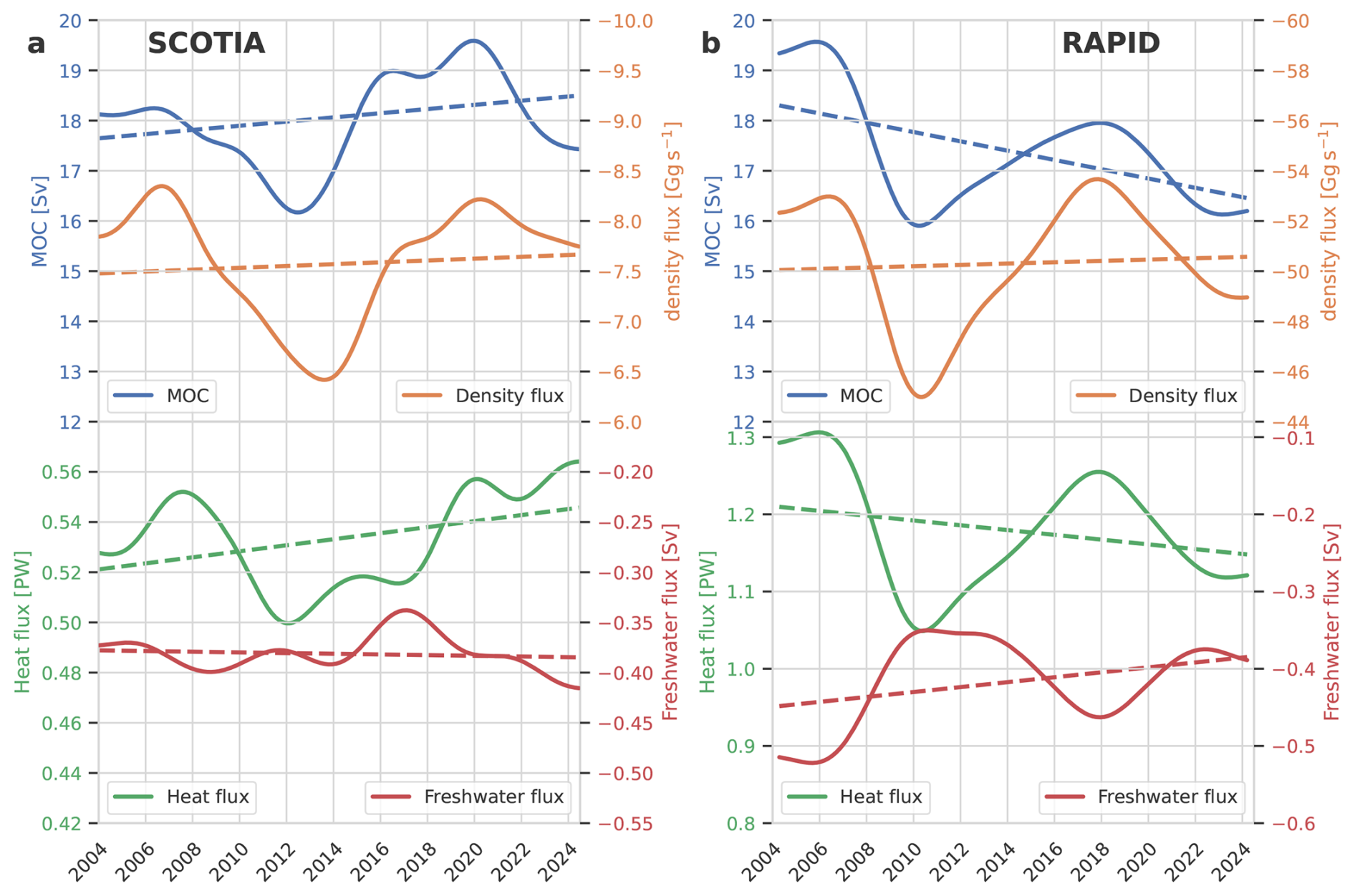
Figure 7 Time series of 5 year low-pass filtered MOC, northward density flux 𝒟, northward heat flux ℋ, and northward freshwater flux from (a) SCOTIA and (b) RAPID. Dashed lines show the corresponding linear trends. Note that we have reversed the y axis scale for density flux to emphasise the similarity to MOC variability.

Pentadal to decadal variability of density flux, as for the shorter timescales, follows the same pattern as MOC, with increased southward density flux at times of increased MOC. This same pattern is seen in the northward heat flux, though slightly modified at SCOTIA by the greater freshwater influence. Variability in freshwater flux at RAPID on these longer timescales tends to oppose the density flux and MOC variability, which are both dominated by temperature. In contrast, at SCOTIA, there are periods where heat fluxes dominate the density flux and MOC variability (e.g. 2008–2012, 2017–2019) and other periods where freshwater fluxes appear dominant (e.g. 2014–2016).

Deep and overflow waters play a crucial role in the overturning circulation, these lower limb waters occupy depths from the depth of γ_MOC down to over 5000 m, and neutral densities from 27.75 to 28.1 kg m⁻³. South of around 40–50° N the deep, southward-flowing watermasses are generally separated into upper and lower North Atlantic Deep Water (uNADW and lNADW). These watermasses in turn are primarily formed from overflow waters (Denmark Strait Overflow Water, DSOW; Iceland–Scotland Overflow Water, ISOW) and Labrador Sea Water (LSW) by intense mixing processes in the region 40–50° N (e.g. Liu and Tanhua, 2021; Lozier et al., 2022). DSOW and ISOW, originating in the Arctic Ocean, mix to form the majority of the lNADW; while LSW, formed in the Labrador Sea, comprises a major part of uNADW.

Precise definitions of these deep water masses can be complex, involving overlapping ranges of density, depth, temperature, salinity and oxygen and nutrients, which might also change with time. Here we use simplified definitions, based purely on neutral density ranges, estimated by comparison with depth and density ranges quoted in the literature (e.g. Smeed et al., 2014; Zantopp et al., 2017; Liu and Tanhua, 2021; Lozier et al., 2022; Yashayaev, 2024). These ranges, in kg m⁻³, are: at SCOTIA – upper LSW $\mathrm{27.78}<\mathit{\gamma }<\mathrm{27.88}$, lower LSW $\mathrm{27.88}<\mathit{\gamma }<\mathrm{27.98}$, ISOW $\mathrm{27.98}<\mathit{\gamma }<\mathrm{28.08}$, DSOW γ>28.08; and at RAPID – uNADW $\mathrm{27.75}<\mathit{\gamma }<\mathrm{28.08}$, lNADW $\mathrm{28.08}<\mathit{\gamma }<\mathrm{28.14}$, northward-flowing Antarctic bottom water close to the bed (AABW) γ>28.14.

We now apply the same 5 year low-pass filter to the lower limb volume transport time series (Fig. 8). By construction, the total lower limb transports and MOC (Fig. 8a and b) differ only in sign and in the transports being referenced to a fixed density rather than a time-varying density as for MOC. Splitting the lower limb into lighter upper (Fig. 8c) and denser lower (Fig. 8d) categories, reveals that at both SCOTIA and RAPID the observed MOC variability pattern is largely coming from the denser waters. That is the lNADW at RAPID and waters with γ>27.98 at SCOTIA. For RAPID this corresponds with previously published results (Smeed et al., 2014), however observations of overflow transports find them to be fairly constant so this appears a surprising result for SCOTIA.

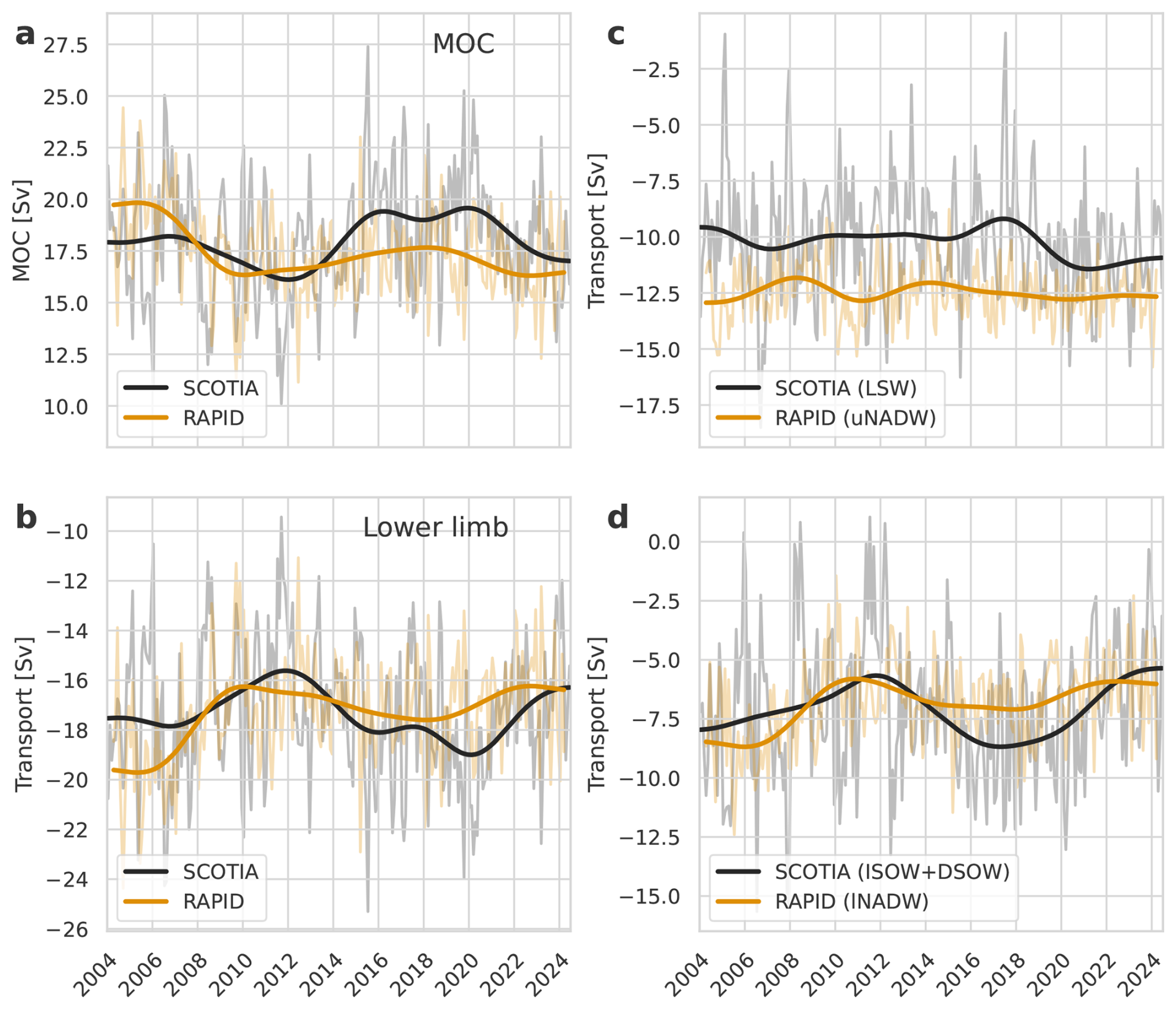
Figure 8 Time series of overturning and watermass transports at SCOTIA (black lines) and RAPID (amber lines). The paler lines show the monthly time series, these differ from those in Fig. 5 in that the seasonal cycle and surface Ekman driven components have been removed. The darker lines show the results from a 5 year low-pass filter. Panel (a) MOC. (b) lower limb transports, these differ from MOC in that they are referenced to the mean, rather than monthly, γ_MOC. RAPID lower limb includes AABW transport. (c) The lighter part of the lower limb transport (LSW at SCOTIA and uNADW at RAPID). (d) the denser part of the lower limb transport (DSOW and ISOW at SCOTIA, and lNADW at RAPID). See the text for the watermass definitions used.

We display in Fig. 9 density space transports accumulated over both the upper and lower MOC limbs from zero transport at γ_MOC. This novel way of visualising the evolution of the density-space overturning streamfunction emphasises transport variability within density classes. For overturning transports at RAPID, we find (Fig. 9b) that in the lower limb the step change in overturning transports is centred on waters of neutral density $\mathrm{28.10}<\mathit{\gamma }<\mathrm{28.13}$ kg m⁻³, this water is at depths of 4000–5000 m. The corresponding signal in the upper limb shows as a reduction in northward transport in the density range $\mathrm{26.2}<\mathit{\gamma }<\mathrm{27.0}$ kg m⁻³, that is about 200–600 m depth. Upper limb waters of this density sit around the local minimum in Fig. 6, that is the overlap region between subtropical gyre and deep overturning cells described in Tooth et al. (2024), or the subtropical recirculating downward spiral of Berglund et al. (2022) preceding the northward advection of water particles to the subpolar regions. Notably, the net northward transport of water with density less than 26.2 kg m⁻³ remains quite constant throughout the period. This again reflects the idea described earlier when considering overturning and density fluxes, that if the subtropical overturning is considered as the superposition of two cells – a shallow subtropical recirculation and a deep recirculation via subpolar and polar ocean – the variability is primarily seen in the deep recirculation.

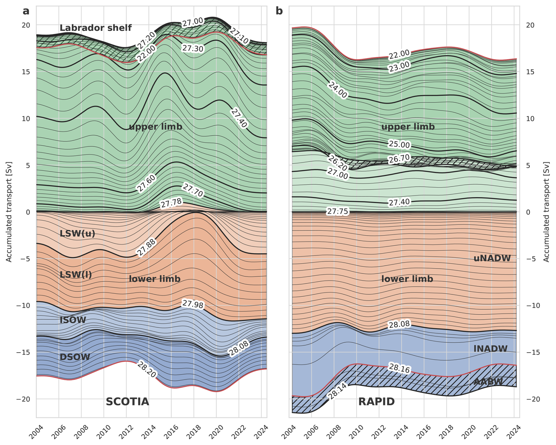
Figure 9 Time series of 5 year low-pass overturning streamfunction at (a) SCOTIA and (b) RAPID plotted as northward transport (y axis) in the density range between γ and γ_MOC. Transport in any density range is shown by line spacing, wider line spacing show density ranges and times of stronger transport. So parallel lines show largely constant transport, lines that aren't parallel show transports changing with time. In the upper, green shaded regions, hatched regions are density ranges with net southward transport. These are confined to the lightest, Labrador shelf water on SCOTIA, and to a density range of about 26.2–26.7 kg m⁻³ for RAPID (see Fig. 6). In the lower, amber and blue shaded regions, hatched regions have net northward transport. This is confined to the AABW at γ>28.20. Where contours cross the zero line (2014–2020 at SCOTIA) indicates periods where γ_MOC is notably different from the long term mean.

For SCOTIA (Fig. 9a), we see more transport variability than at RAPID. The most prominent feature of the SCOTIA low-frequency overturning transport time series is the increased southward transport of the denser class of Labrador Sea Water (LSW(l)) between 2014–2022. Yashayaev (2024) provides a time series of the formation of LSW via deep convection in the central Labrador Sea, detailing the many drivers of convection depth and LSW density as well as the appearance of the LSW downstream in the Labrador Sea outflow. The time evolution of the 5–10 year MOC we observe at SCOTIA looks extremely similar to that of central Labrador Sea convection depth (Fig. 4 of Yashayaev, 2024). So why do our results in Fig. 8d suggest the source of this signal lies mostly in the deep overflow waters? This is partly because Fig. 8d shows only the total LSW transport (the sum of LSW(u) and LSW(l)), whereas Fig. 9a reveals that the increased southward transport of LSW(l) is compensated by a reduced, or even northward, transport of LSW(u). This is also likely an artefact of our LSW definition occupying a fixed density range, since LSW production shows significant variation in density, the 2014–2018 period showing production of some of the densest classes of LSW seen since the early 1990s (Yashayaev, 2024).

Finally we return to the high γ_MOC at SCOTIA in the period 2014–2020 (Fig. 5c). We see this in Fig. 9 as the protrusion of LSW into the “upper limb” of the circulation. This again coincides with the production of more, and denser, LSW through deep convection in the central Labrador Sea. As this water leaves southward in the Labrador Sea outflow, it results in shoaling of the isopycnals in the outflow (Fox et al., 2022) and a resulting shift in γ_MOC to higher density to maintain volume transport balance. This is consistent with modelling results of Petit et al. (2025) who show that the density at which the maximum overturning occurs at OSNAP is linked to an atmospherically driven shoaling of isopycnals. This shoaling then propagates along the western boundary, taking about a year to reach 45° N, and is a key precursor of mid-latitude AMOC strength.

5 Discussion

Here, we have demonstrated that SCOTIA provides an overturning structure and variability consistent with that from the full OSNAP array. Crucially, because many of the observations used extend back to the mid-2000s, SCOTIA provides a 20 year record of subpolar overturning: the first sustained observational view of decadal AMOC variability at subpolar latitudes.

We find no statistically significant MOC decline in the 20 year SCOTIA record. This result can be compared with studies suggesting limited long-term change in subpolar overturning since the 1990s (e.g. Fu et al., 2020), although differences in time period and methodology mean that the results are not directly comparable. The lack of a trend is not unexpected, given that the MOC at SCOTIA displays greater variability than at RAPID, where the time window required to detect a trend is estimated to be 14–42 years (Lobelle et al., 2020). Thus, the lack of clear evidence for a trend should not be interpreted as evidence against the anthropogenic MOC decline suggested by proxies (Caesar et al., 2021) and models (Weijer et al., 2020).

What does it mean for MOC to decline at RAPID but not at SCOTIA? There is little if any outcropping of the γ_MOC isopycnal between the two sections, so little direct surface-driven transformation from upper to lower limb. Therefore, the difference in MOC must be balanced either by dense water accumulation or by changes in diapycnal mixing within that region over the past 20 years.

The SCOTIA product provides new observational insights into how transports in different density classes impact subpolar overturning and transport evolution on longer (pentadal- to decadal-scale) time scales. This longer time series allows us to identify that the subpolar MOC during 2016–2020 was anomalously high, and was associated with both an increased γ_MOC and an increased southward transport of lower Labrador Sea Water. This period broadly coincides with progressively deeper convection in the Labrador Sea during 2012–2018 generating an anomalously large and dense class of Labrador Sea Water (Yashayaev, 2024). This process both transforms more water from upper to lower limb densities and rearranges the vertical structure within the lower limb. The additional transformation causes shoaling of isopycnals in the strong southward-flowing western boundary current, reducing southward flow in the upper limb and shifting γ_MOC to higher density to retain mass balance. We expect the increased lower limb density at the western boundary to also impact the dynamic height gradients across the subpolar North Atlantic, accelerating the upper limb. Labrador Sea convection controlling AMOC variability over these timescales is suggested by recent modelling results (Yeager et al., 2021), and we here establish the first observational evidence for this mechanism.

The observations of decadal-scale variations in γ_MOC at SCOTIA also represent the first such observations in subpolar overturning, observations which have been enabled by the extended length of the SCOTIA time series. Modelling work (Petit et al., 2025) has identified this subpolar γ_MOC variability as a key precursor to overturning in mid-latitudes.

SCOTIA offers an alternative configuration for observing subpolar AMOC and the associated heat and freshwater fluxes. By omitting observations of the boundary currents around Greenland, the SCOTIA methodology cannot discriminate between convection in the Irminger and Labrador Basins (e.g. Lozier et al., 2019; Li et al., 2021; Fu et al., 2023a, 2025), resolve freshwater fluxes on the shelf and slope either side of Greenland (e.g. Le Bras et al., 2018), or capture signals in the overflow transports immediately downstream of the Greenland–Scotland Ridge (e.g. Pacini et al., 2020; Foukal and Pickart, 2023; Koman et al., 2024; Sun et al., 2025). SCOTIA should not, therefore, be considered a substitute for the OSNAP array, which resolves these features, but rather an additional, partially independent measure of subpolar overturning with the advantage of providing a longer-term perspective. There are, however, increasing pressures to make ocean observing more sustainable, as reflected by changes to funding landscapes and government priorities across the North Atlantic towards reduced ship-time, lower emissions, and greater use of autonomous and low-cost platforms. Under these constraints, it is far from clear that the present AMOC monitoring infrastructure can be maintained in the long term. The approach presented here might provide a useful template for a lightweight and sustainable subpolar AMOC observing system for the coming decades.

The degree of independence between SCOTIA and OSNAP warrants careful interpretation. Although SCOTIA draws on a subset of OSNAP moorings and shared reanalysis products (ERA5 and GLORYS), it employs a distinct methodological framework. Notably, SCOTIA infers geostrophic currents over sloping boundaries rather than relying on direct velocity observations, uses time-varying altimetric referencing, and adopts an alternative compensation strategy. In this sense, SCOTIA provides a novel assessment of subpolar overturning from partially overlapping data. However, elements of the SCOTIA methodology, such as the spatial structure of the compensation velocity and the treatment of shelf regions, have been selected for consistency with OSNAP. Consequently, correlations between the two time series should not be interpreted as arising from wholly independent analyses.

The 20 year SCOTIA record presented here offers a unique opportunity to enhance our understanding of decadal-scale variability in the subpolar North Atlantic and its relationship with climate. Further work is required to better understand how variability in the overturning and fluxes observed at SCOTIA related to key climate metrics (e.g. NAO index) and regional ocean conditions (e.g. sea surface height and temperature). The longer time series also provides the opportunity to better assess how well ocean and climate models represent decadal modes of variability.

Our methodology allows near-real-time updates to be generated based on the latest Argo and satellite data, with a refined delayed-mode analysis following mooring recovery, reducing uncertainty in the final fields. The simplified array design also makes near-real-time mooring telemetry across the full array a realistic ambition, paving the way for a high-fidelity “AMOC live stream”.