Sea-surface temperature variability and climate drivers in Cuba's Jardines de la Reina National Park (2003–2022)

Coral reef systems on the southeastern Cuban shelf are exposed to rapid warming and increasingly frequent marine heatwaves (MHWs). However, the physical drivers of local sea-surface temperature (SST) variability remain poorly quantified. The present study examines seasonal-to-decadal SST variability in and around the Jardines de la Reina National Park (JRNP) and investigates the extent to which atmospheric–ocean processes and large-scale climate modes influence that variability. The study analyses daily 1 km Multi-Scale Ultra High Resolution (MUR) SST from 2003–2022, in conjunction with ERA5 surface heat fluxes and GLORYS12 mixed-layer fields. A mixed-layer heat budget, compiled from daily values and averaged to monthly values, is used to attribute the seasonal cycle; long-term trends, MHWs and modes of variability (Empirical Orthogonal Funtions – EOFs) can be used to explain interannual to decadal changes and their links to El Niño Southern Oscillation (ENSO), the Western Hemisphere Warm Pool (WHWP), the Tropical North Atlantic (TNA) and the North Atlantic Oscillation (NAO).

Net air–sea heat exchange sets the seasonal evolution of SST, whereby horizontal advection provides a smaller modulation near the shelf break; a characteristic ∼2-month lead of heat flux over temperature is consistent with mixed-layer heat storage. This thermodynamic control explains a marked autumn–winter shelf–offshore contrast between the shallow gulfs (Gulfs of Ana María – GAM and Guacanayabo – GG) and the adjacent Caribbean Sea. Superimposed over this area is a warming trend of ∼0.28 °C per decade (strongest in winter/transition months, peaking around April at ∼0.48 °C and November at ∼0.35 °C per decade) and a step-like shift in 2011–2013 towards a persistently warmer state. MHWs intensified during the second decade; the mean event-wise maximum intensity was higher inside GAM, while upper categories occurred more frequently offshore. EOF1 (87.5 %) is a basin-wide mode linked on an interannual basis to ENSO/WHWP and latent-heat flux and at low frequency to the NAO, while EOF2 (6.2 %) captures a shelf–offshore dipole related to TNA.

Our results provide a physical basis for which to issue early warnings from forecasts of net heat flux and mixed-layer depth, thus encouraging the use of regional high-resolution modeling and targeted observations. Key limitations to the present study include a 20-year MHW baseline and an under-resolution of currents in highly shallow and complex bathymetry.

1 Introduction

Sea surface temperature (SST) is a key regulator of marine ecosystems, since it drives physical, chemical and biological processes. Its variability has profound implications for coastal and oceanic regions in a warming climate (Venegas et al., 2023). Since the industrial era, anthropogenic pressures have altered ocean dynamics and accelerated habitat degradation (Jackson et al., 2014; Lotze et al., 2006). Rising SSTs are closely linked to coral bleaching, habitat fragmentation and biodiversity loss in tropical regions (Bruno et al., 2019; Hughes et al., 2003). Coral reef ecosystems are susceptible to temperature fluctuations and to co-occurring stressors, including light, sedimentation and chemical changes (Cramer et al., 2020). As a result, understanding the patterns and drivers of SST variability has become crucial in order to predict ecological impacts and inform conservation efforts.

The Caribbean Sea (CS) hosts extensive coral reefs and numerous marine protected areas (MPAs), which are central to regional conservation and livelihoods. The Jardines de la Reina National Park (JRNP), the largest marine reserve in Cuba and one of the largest in the Caribbean, is notable due to its exceptional reef conditions and biodiversity (Appeldoorn and Lindeman, 2003; Linton et al., 2002; Gerhartz-Muro et al., 2018). Yet, JRNP faces a number of challenges typical of Caribbean reefs, including the dramatic decline of historically dominant species, such as Acropora palmata, now classified as critically endangered (Caballero-Aragón et al., 2020). Prior work at JRNP has focused primarily on reef ecology and conservation status (Hernández-Fernández et al., 2011, 2016, 2019; Pina-Amargós et al., 2008), with fewer studies addressing the physical drivers that modulate local thermal stress and ecosystem vulnerability. This research gap is significant, since thermal extremes and the persistence thereof increasingly govern the risk of coral bleaching across the region (van Hooidonk et al., 2015; Graham et al., 2015; Mumby et al., 2014).

At a broader scale, southern Cuba exhibits warmer SST than the northern shelf of the island, influenced by exchanges with the CS (Cerdeira-Estrada et al., 2005; Chollett et al., 2012; Caravaca et al., 2022; González-De Zayas et al., 2022). Basin-wide analyses also point to a significant warming trend during recent decades, which are particularly pronounced to the south of Cuba (Avila-Alonso et al., 2020). However, existing studies provide merely a partial view of SST variability on the southeastern Cuban shelf and seldom disentangle the relative roles of air–sea heat fluxes, horizontal advection and large-scale climate modes in shaping local conditions within and adjacent to JRNP.

Large-scale atmospheric variability modulates Caribbean SST through several well-documented pathways. The El Niño Southern Oscillation (ENSO) influences trade winds and latent heat flux over the Western Hemisphere Warm Pool (WHWP), defined as the region warmer than 28.5 °C in the Western Tropical Atlantic and in the eastern North Pacific, which alter regional SST at interannual scales (Wang and Enfield, 2001, 2003; Czaja et al., 2002). The North Atlantic Oscillation (NAO) affects wind patterns, precipitation and heat exchange across the North Atlantic–Caribbean system, including via the Caribbean Low-Level Jet (Hurrell, 1995; Wang et al., 2007; Cook and Vizy, 2010). Additional variability arises from the Tropical North Atlantic (TNA) and WHWP indices, which capture shifts in regional SST (Enfield et al., 1999; Enfield and Lee, 2005). The process of clarifying how these climate modes project onto local SST in the shelf versus adjacent oceanic waters near JRNP is crucial for efforts to link physical forcing with ecological risk.

In the present study, we investigate seasonal-to-decadal variability of sea-surface temperature in and around JRNP and its controlling mechanisms using daily 1 km Multi-Scale Ultra High Resolution (MUR) SST (2003–2022), ERA5 dataset surface heat fluxes, and GLORYS12 (1/12°) dataset currents/temperature by: (i) resolving the seasonal cycle and diagnosing the mixed-layer heat budget to gauge air–sea heat exchange versus horizontal advection; (ii) quantifying long-term trends and testing for regime shifts; (iii) detecting and characterizing marine heatwaves (MHWs); and (iv) extracting dominant modes via Empirical Orthogonal Functions (EOFs) and relating them to the ENSO, the NAO, the TNA, and the WHWP.

Accordingly, we address three working hypotheses: (1) at seasonal scales, air–sea heat fluxes dominate SST variability, with shallow shelf waters exhibiting stronger amplitude and faster cooling/warming than adjacent oceanic waters; (2) interannual variability shows modulation by ENSO/WHWP and TNA via latent-heat-flux anomalies and circulation changes; and (3) decadal changes in the region, including post-2010 regime shifts, are consistent with NAO-related variations in atmospheric forcing. By resolving shelf–offshore contrasts and attributing variability across time scales, the analysis herein provides a physical basis for interpreting recent and future thermal stress in this MPA in addition to anticipating ecosystem responses under continued warming.

2 Data and methods

2.1 Study region: Jardines de la Reina National Park

The JRNP lies on the southeastern Cuban shelf, bordered to the north by the Gulf of Ana María (GAM), to the east by the Gulf of Guacanayabo (GG) and to the south by the CS (Fig. 1). The archipelago comprises ∼661 cays (keys) that extend east–west and which are fringed by mangroves. According to Pina-Amargós et al. (2008), the protected area covers 217 036 ha, of which 200 957 ha are marine hectares. The seafloor shows a marked north–south contrast: to the north, the shallow GAM is characterized by extensive flat banks, seagrass beds and soft sediment with a general depth of <20 m; to the south, the shelf edge transitions abruptly to a steep continental slope descending to >3000 m. This sharp gradient underpins a mosaic of habitats, from shallow coastal ecosystems to deep-sea environments.

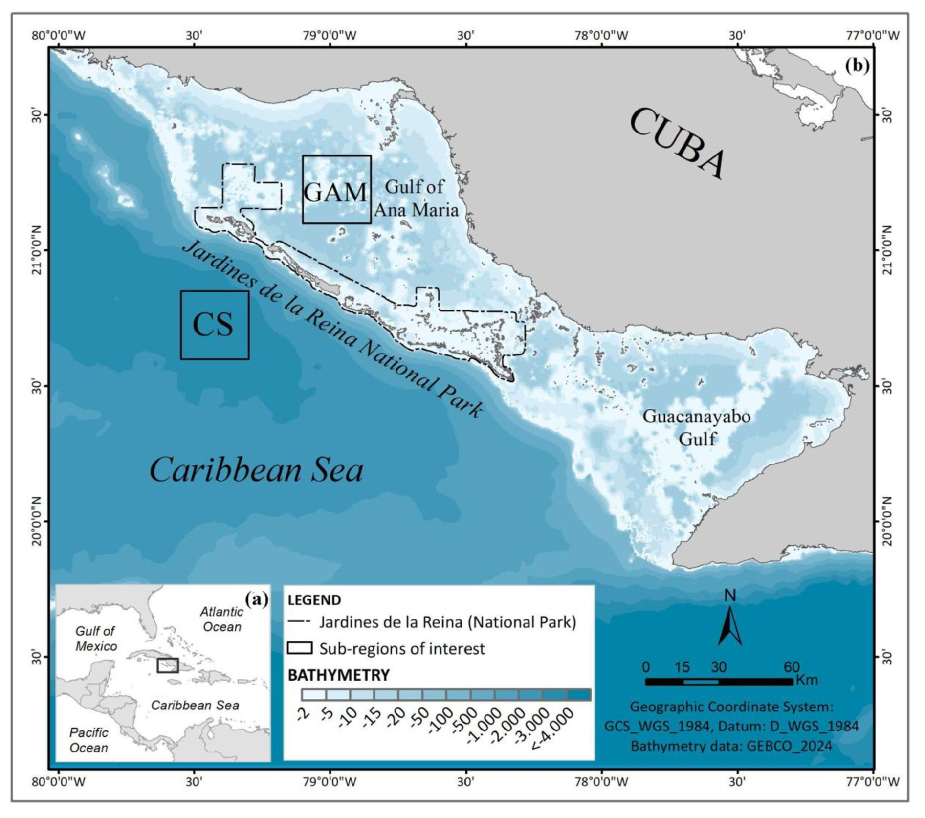
Figure 1 Study area and sub-regions. (a) Regional setting: Cuba in the Caribbean Sea (CS), with the study domain indicated by the black rectangle. (b) Southeastern Cuban shelf showing the Jardines de la Reina National Park (black polygon) and neighbouring gulfs: Gulf of Ana María (GAM) and Gulf of Guacanayabo (GG). Black boxes mark the two analysis sub-regions: GAM (shelf) and CS (oceanic). Colour shading shows bathymetry (m) from GEBCO_2024.

The region has a tropical climate with two boreal seasons: a wet season (May–October) and a dry season (November–April). Prevailing trade winds are generally northeasterly and strengthen during the dry season (Pérez-Santos et al., 2010). Sea-level pressure follows a seasonal cycle, with higher values in boreal winter (January–March) under the influence of the subtropical high, and lower values in summer (July–September) as the intertropical convergence zone approaches (Waliser and Jiang, 2015). Air temperatures are warm year-round (∼24–30 °C) and there is modest interannual variability, despite pronounced diurnal and seasonal cycles. Summer is warmest while winter is slightly cooler (Caravaca et al., 2022). On the southeastern Cuban shelf, the mean flow is westward under the prevailing easterlies (Emilsson and Tápanes, 1971). It is modulated by tides and currents from the adjacent ocean, notably the Caribbean Current Arriaza et al., 2008). Tides are mixed and exert little direct control on the mean shelf circulation, although tidal currents can enhance vertical mixing (Emilsson and Tápanes, 1971; Arriaza et al., 2008).

2.2 SST data

Sea-surface temperature was obtained from the Group for High Resolution Sea Surface Temperature MUR Level-4 analysis produced by the NASA Jet Propulsion Laboratory. This product provides daily global fields at ∼1 km (0.01°) by blending multiple infrared and microwave satellite sensors (Chin et al., 2017) and is widely used in tropical reef and coastal studies (for example, Kumagai and Yamano, 2018; Skerrett et al., 2024). The present study analyzed data from 2003 to 2022 and subsequently subset the domain, as shown in Fig. 1.

All processing was performed on the native 1km grid, unless otherwise specified. Daily fields were: (i) land-masked and quality-screened using the product masks; (ii) averaged to monthly means for the long-term, seasonal and EOF analyses; and (iii) converted to monthly anomalies by removing the 2003–2022 monthly climatology (further details are provided in Sect. 2.5). For diagnostics requiring co-location with reanalyses (mixed-layer heat budget and horizontal advection), SST was bilinearly remapped to the target grid (GLORYS12 at 1/12° or ERA5 at 1/4°) to avoid artificial gradients from mismatched resolutions. All temperatures are reported in °C.

We retained the 1 km fields to show frontal structures in Fig. 2; frontal overlays are computed from local SST differences (threshold ≥ 0.5 °C) and lightly smoothed with a 3×3 neighbourhood operator to suppress pixel-scale noise.

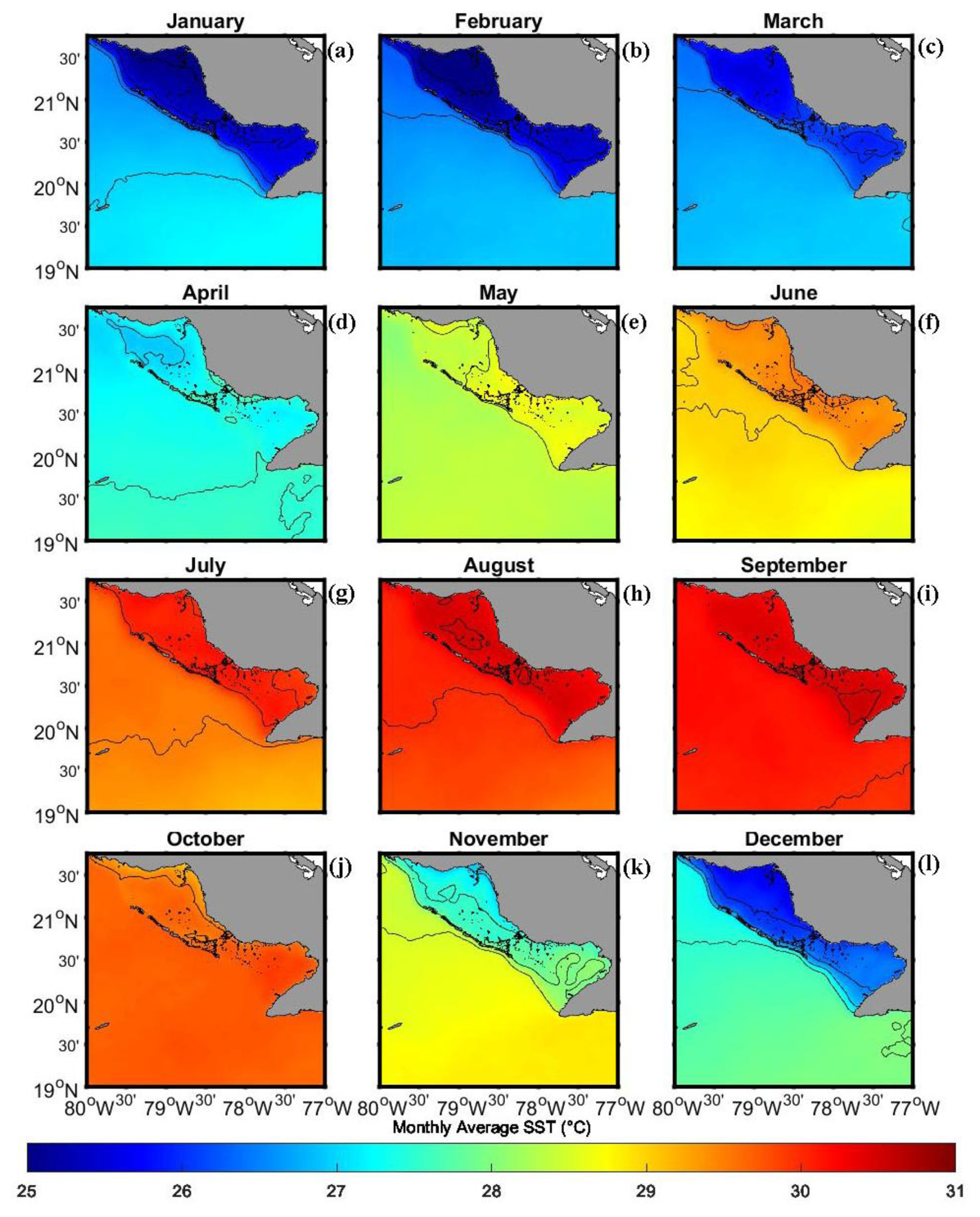
Figure 2 Monthly SST climatology (based on period 2003–2022). Panels (a)–(l) show monthly mean sea-surface temperature (°C) from January to December. Black contours mark SST fronts identified, where local horizontal SST differences are ≥0.5 °C. Seasonal groupings are: (a–c) boreal winter (JFM), (d–f) spring (AMJ), (g–i) summer (JAS), and (j–l) autumn (OND). The colour bar indicates monthly mean SST (°C); land is masked in grey.

It should be noted that MUR SST was not used in the mixed-layer heat budget (Sect. 2.6); there, we diagnosed temperature tendencies ($\partial T/\partial t$) using the GLORYS12 mixed-layer temperature (MLT), depth and currents for reasons of internal consistency with regards to the terms. At monthly scales, MUR SST and GLORYS12 MLT were correlated throughout the study area, thus, variability in MLT is interpreted as the explanation for the observed SST variability.

To assess the internal consistency of the SST variability represented by the different products used in this study, we performed a quantitative intercomparison between MUR SST, ERA5 SST, and GLORYS12 MLT over the full analysis domain and period (2003–2022). The agreement is summarized in Sect. S1 in the Supplement (Fig. S1 in the Supplement) using a Taylor diagram (correlation, normalized standard deviation, and centered RMSD referenced to MUR), which provides an objective measure of how well the coarser-resolution products reproduce the temporal variability and amplitude of the satellite-based SST anomalies. In addition, an independent consistency check using short-term in situ temperature time-series available within the Jardines de la Reina region is presented in Fig. S2. Although these comparisons do not constitute a full in situ validation for the region, they support the suitability of MUR SST for describing spatial and temporal variability and provide a transparent characterization of cross-product differences relevant to the interpretation of our results.

2.3 Atmospheric fluxes and ocean reanalysis

The present study used ERA5 surface flux components (shortwave, longwave, latent and sensible) and 10 m winds at native hourly resolution, aggregated to daily and then monthly means for the period 2003–2022. The upper-ocean state was characterized with GLORYS12 at daily resolution (temperature, horizontal currents and Ocean Mixed Layer Thickness), with monthly means used for non-budget diagnostics. Heat flux was measured in W m?⁻². The oceanographic convention that holds that positive net heat flux warms the ocean was adopted throughout the course of the present research.

The upper-ocean state was characterized by GLORYS12 (eddy-resolving, 1/12°, 50 vertical levels, daily), from which potential temperature, horizontal currents and mixed layer depth and temperature were extracted over the same period. Fields were subset to the domain shown in Fig. 1 and, where necessary, bilinearly remapped to a standard grid (ERA5-GLORYS12) for the mixed-layer heat budget and advection diagnostics. Regarding the budget, ERA5 fluxes were first aggregated to daily values and then bilinearly remapped to the GLORYS12 grid; the results were subsequently averaged to a monthly basis. For descriptive analyses, monthly fields were utilized.

2.4 Climate indices

The present study used a monthly time series of large-scale climate indices known to modulate Caribbean SST. The ENSO was represented by the Multivariate ENSO Index v2 (MEI.v2) (Zhang et al., 2019; Wolter, 1993), obtained from the NOAA Physical Sciences Laboratory (PSL). The WHWP index (Wang and Enfield, 2001, 2003; Enfield and Lee, 2005; Wang et al., 2006) and the TNA index (Enfield et al., 1999; Chen et al., 2021) were also taken from NOAA PSL. The NAO index was obtained from the NOAA Climate Prediction Center (CPC) (Barnston and Livezey, 1987; Chen and Van den Dool, 2003; Van den Dool et al., 2000).

All indices were analyzed at monthly resolution pertaining to the period 2003–2022, to match the SST analysis period. Prior to correlation and filtering analyses (Sect. 2.9), each index was standardized (zero mean, unit variance) over the 2003–2022 period. Provider sign conventions were retained.

2.5 Statistical analysis

All analyses were performed over the domain 19–21.75° N, 77–80° W (Fig. 1). Land points were masked. Daily fields were aggregated to monthly means, while monthly anomalies were computed by removing the 2003–2022 monthly climatology. Unless otherwise specified, statistics refer to the aforementioned monthly anomalies.

Long-term monthly means were used to show the seasonal cycle of SST and surface heat fluxes (Figs. 2–4). To contrast shelf and offshore regimes, we computed time series over the two small boxes shown in Fig. 1: GAM (shelf) and CS (oceanic). For each box, monthly anomalies, standard deviations and seasonal composites were calculated. To verify that our GAM and CS time series are not sensitive to the exact choice of box location and size, we repeated the analysis using multiple alternative boxes within GAM and offshore in the CS (Sect. S2, Fig. S3). The resulting SST-anomaly time series remain highly consistent with the reference series (all correlations significant at ≥95 % confidence; Table S1 in the Supplement), indicating that the reported shelf–offshore contrasts are robust to reasonable variations in box definition.

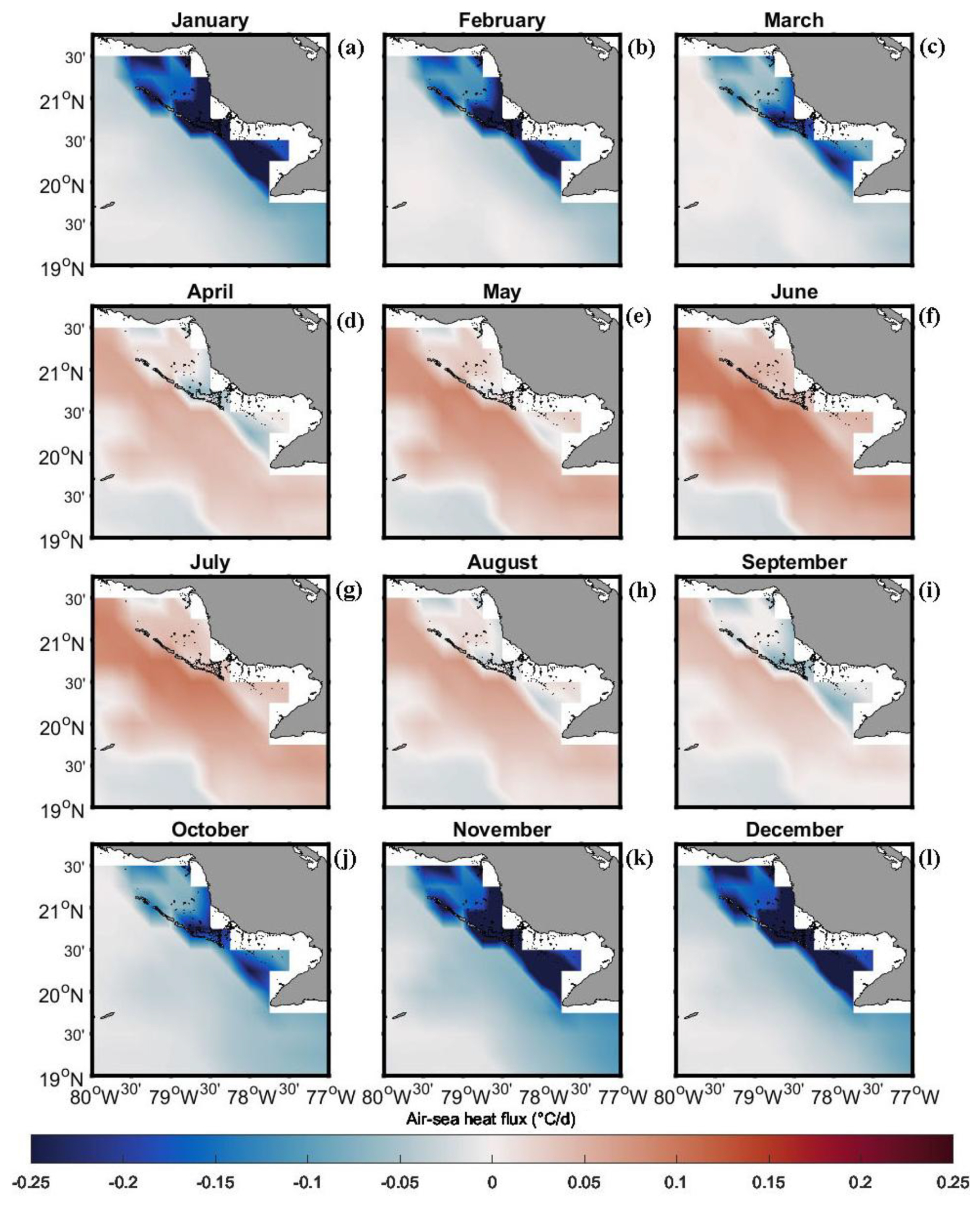
Figure 3 Monthly air–sea heat-flux tendency term. Panels (a)–(l) show the monthly mean mixed-layer heating rate due to net air–sea heat exchange, expressed as °C d⁻¹ and computed as $(\partial T/\partial t){\mathrm{|}}_Q=Q_{\mathrm{net}}/\left(\mathit{\rho }{C}_{\mathrm{p}}h\right)$. Positive (red) warms the ocean; negative (blue) cools the ocean. Months run January–December; seasonal groupings are (a–c) boreal winter (JFM), (d–f) spring (AMJ), (g–i) summer (JAS), and (j–l) autumn (OND). Flux components are from ERA5, mixed-layer depth h from GLORYS12 all variables are for the period 2003–2022; land is masked in grey.

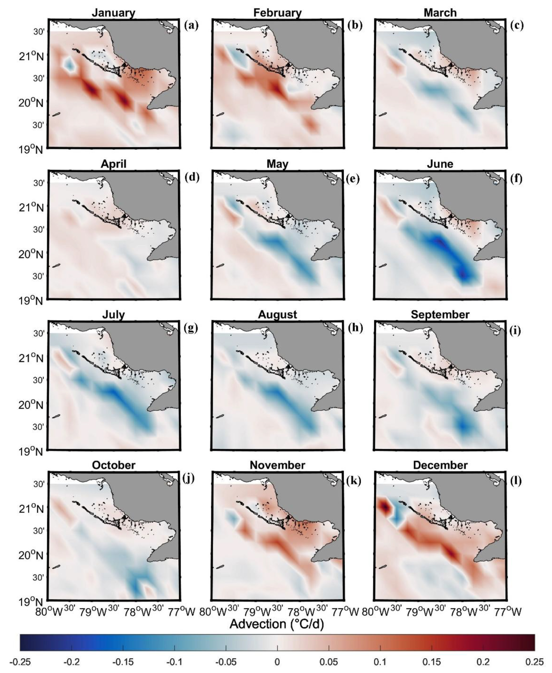
Figure 4 Monthly horizontal heat-advection tendency term. Panels (a)–(l) show the monthly mean mixed-layer temperature tendency due to horizontal advection, expressed as °C d⁻¹ and computed as $(\partial T/\partial t){\mathrm{|}}_{\mathrm{adv}}=-\mathit{U}\cdot \mathrm{\nabla }T$. Positive (red) warms the mixed layer; negative (blue) cools it. Currents and temperature gradients are from GLORYS12 (ML-averaged currents and mixed-layer temperature) all variables are for the period 2003–2022; land is masked in grey.

Linear trends were estimated using ordinary least squares applied to monthly anomalies at each grid point, separately for each calendar month. Slopes are reported in °C per decade. Statistical significance was assessed at the 95 % level using a two-sided Student's t test. To account for serial autocorrelation inherent in geophysical time series, we calculated the effective degrees of freedom (N^*) following the approximation by Thomson and Emery (2024). N^* was estimated using the lag-1 autocorrelation coefficient (r₁):

$$\begin{array}{}\text{(1)}& N^{*}=N{\displaystyle \frac{\mathrm{1}-\mathrm{|}{r}_{\mathrm{1}}\mathrm{|}}{\mathrm{1}+\mathrm{|}{r}_{\mathrm{1}}\mathrm{|}}}.\end{array}$$

Thus, the significance tests for trends and correlations use an effective degrees-of-freedom estimate, yielding more conservative p values under serial correlation.

To quantify coupling between SST and different drivers, cross-correlations between SST anomalies and net surface heat flux were computed (and, where relevant, horizontal heat advection; Sect. 2.6) using monthly data, by scanning lags from −6 to +6 months. Reported lags correspond to the peak absolute correlation. Significance was evaluated using the t test for the correlation coefficient and the effective degrees of freedom approach. Where budget terms are summed (Sect. 2.6; Fig. 5), the uncertainty of the sum was obtained by root-sum-of-squares, assuming weak covariance between terms at monthly resolution. All computations and figure generation were carried out via the MATLAB computing platform using standard scientific libraries.

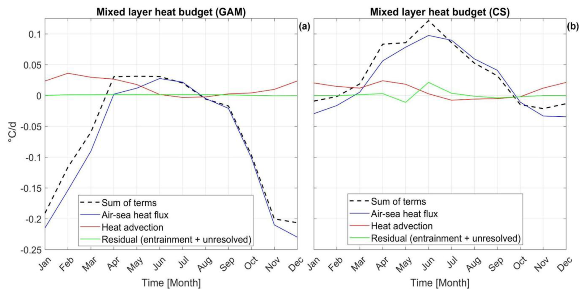
Figure 5 Seasonal mixed-layer heat budget (2003–2022). Monthly climatologies of mixed-layer temperature tendencies (°C d⁻¹) for (a) GAM and (b) CS. Blue line: air–sea heat-flux tendency $(\partial T/\partial t){\mathrm{|}}_Q=Q_{\mathrm{net}}/\left(\mathit{\rho }{C}_{\mathrm{p}}h\right)$. Red line: horizontal advection $(\partial T/\partial t){\mathrm{|}}_{\mathrm{adv}}=-\mathit{U}\cdot \mathbf{\nabla }T$. Dashed black line: sum of resolved terms (flux + advection). Green line: residual (entrainment + unresolved processes), computed as the observed mixed-layer temperature tendency minus the sum of resolved terms. Positive values warm the mixed layer; negative values cool it. All terms were computed from daily fields and averaged to monthly means; see Sect. 2.6 for data sources and sign conventions.

2.6 Mixed-layer heat budget

To identify the processes governing the seasonal variability of SST, we applied a standard mixed-layer (ML) heat budget (for example, Moisan and Niiler, 1998). Since the budget is defined in relation to the bulk mixed layer, the GLORYS12 MLT and mixed-layer depth (MLD) were used to ensure physical and numerical consistency among terms (flux → heating rate via h; advection using currents acting on the same temperature field). At monthly scales, MUR SST and GLORYS12 MLT were well correlated over the domain (Sect. 2.2), Therefore, accounting for MLT variability was taken as providing an explanation for the observed SST variability.

The prognostic equation for MLT T is

$$\begin{array}{}\text{(2)}& {\displaystyle \frac{\partial T}{\partial t}}={\displaystyle \frac{Q_{\mathrm{net}}}{\mathit{\rho }{C}_{\mathrm{p}}h}}-\mathit{U}\cdot \mathbf{\nabla }T-{\displaystyle \frac{\left(\frac{\partial h}{\partial t}+{\mathit{U}}_{-\mathrm{h}}\cdot \mathbf{\nabla }h+w_{-\mathrm{h}}\right)\mathrm{\Delta }T}{h}}+R\end{array}$$

where ρ=1025 kg m⁻³ is seawater density, C_p=3990 J kg⁻¹ K⁻¹ is the specific heat capacity, h is the MLD, Q_net is the net downward surface heat flux (into the ocean, W m⁻²),$\mathit{U}=(U,V)$ is the horizontal current vector representative of the ML. The entrainment (positive downward) velocity at the ML base is calculated as follows. The term ${\mathit{U}}_{-\mathrm{h}}\cdot \mathbf{\nabla }h$ represents the contribution to vertical advection associated with horizontal flow (U_−h) moving over an inclined bottom, where U_−h is the horizontal velocity evaluated at the bottom and ∇h the horizontal gradient of the bathymetry, w_−h is obtained by vertically integrating the horizontal velocity divergence from −h to the surface. $\mathrm{\Delta }T=T_{\mathrm{ML}}-T_{\mathrm{below}}$ is the temperature jump across the base of the ML, and R collects unresolved terms (for example, diffusion, sub-monthly variability and analysis noise). All heating rates are reported in °C d⁻¹. Conversion from flux to heating rate follows, whereby

$$\begin{array}{}\text{(3)}& \mathrm{1}\mathrm{W}{\mathrm{m}}^{-\mathrm{2}}\equiv {\displaystyle \frac{\mathrm{86}\mathrm{400}}{\mathit{\rho }{C}_{\mathrm{p}}h}}\mathrm{K}{\mathrm{d}}^{-\mathrm{1}}\end{array}$$

so, for example, with h=20 m, 1 W m${}^{-\mathrm{2}}\sim \mathrm{0.0011}$ °C d⁻¹.

All budget terms were computed from daily fields and then averaged to monthly means for analysis and plots. MLD h was obtained from GLORYS12 “mixed layer thickness”. This estimate is based on a density criterion (Δσ_θ=0.03 kg m⁻³), following the approach proposed by de Boyer Montégut et al. (2004). Daily horizontal velocities from GLORYS12 were vertically averaged from the surface to the local ML base, approximated by thickness-weighted averaging across GLORYS12 levels within the ML.

Surface fluxes (Q_net) were estimated from ERA5 shortwave (SW) and longwave (LW) radiation, latent (LHF) and sensible (SHF) heat fluxes on the 1/4° grid. To reiterate, we adopted herein the oceanographic convention that positive Q_net warms the ocean: $Q_{\mathrm{net}}=(\mathrm{SW}\downarrow -\mathrm{SW}\uparrow )+(\mathrm{LW}\downarrow -\mathrm{LW}\uparrow )-\mathrm{LHF}-\mathrm{SHF}$. The ERA5 native signs (upward positive for turbulent fluxes) are converted accordingly. Fluxes were bilinearly remapped to the GLORYS12 grid prior to the application of Eq. (1).

Horizontal gradients $\partial T/\partial x$, $\partial T/\partial y$ were computed with centered finite differences on the GLORYS12 grid. At a monthly resolution, the flux and advection tendencies in addition to their sum are presented. Furthermore, the entrainment plus unresolved tendency is treated as a residual (for example, the difference between the observed monthly MLT tendency and the sum of resolved terms).

2.7 Marine heatwaves

MHWs were detected from daily 1 km MUR SST data, following the hierarchical definition provided by Hobday et al. (2016, 2018), which contends that an MHW occurs when SST exceeds the seasonally varying 90th percentile threshold for ≥5 consecutive days. For each grid point, we computed a day-of-year (DOY) climatology and corresponding 90th percentile threshold over the period 2003–2022. The DOY climatology and threshold were formed using a ±5 d moving window in order to smooth sampling noise. Events were characterized according to their intensity (absolute anomaly relative to the DOY climatology), duration, frequency, total MHW days and cumulative intensity. MHW categories (Moderate/Strong/Severe/Extreme) were assigned using the factor-of-rule relative to the local threshold exceedance (Hobday et al., 2018).

All diagnostics were computed per grid cell and subsequently summarized for the sub-regions (GAM and CS, Fig. 1). Figure 8 shows the following: (i) maps pertaining to the mean maximum intensity and total MHW days (2003–2022); and (ii) an annual time series of the number of events, mean maximum intensity and maximum category for GAM and CS. It should be noted that the 20-year baseline (2003–2022) used in the present study corresponds to the period during which 1 km MUR SST data were available. Although shorter than the conventional 30-year climatology, the present research does, nevertheless, provide consistent thresholds across the study period. Schlegel et al. (2019) evaluated the impact of time-series length on MHW detection and found that, in general, event durations and intensities derived from a 10-year baseline are not appreciably different from those obtained using a standard 30-year baseline. In addition, to quantify the influence of our 20-year baseline and improve comparability with studies using 30-year climate normals, we performed a sensitivity analysis using GLORYS12, which provides a 30-year record (1993–2022). Following the Hobday et al. MHW definition, we computed MHW thresholds using a 30-year baseline (1993–2022) from GLORYS12 and re-detected MHWs over 2003–2022, then compared the number of days with MHW per year, mean intensity and the standard deviation of the intensity. Results are shown in Table S2. Differences were relatively small, indicating that our conclusions regarding the increase in MHWs during the second decade and the spatial contrasts within JRNP are not sensitive to baseline choice.

2.8 Empirical orthogonal functions

The present study used EOFs to extract the dominant space–time patterns of SST variability over the study domain (19–21.75° N, 77–80° W). The input field was monthly MUR SST anomalies (Sect. 2.2), i.e., monthly means with the 2003–2022 monthly climatology removed. Unless otherwise specified, anomalies time series were not detrended to ensure that the modes were able to capture the interannual–decadal variability previously discussed in Sect. 3.4. For comparison, we also include EOF results computed after removing the linear trend (Fig. S4). All calculations were performed on the native ∼ 1 km grid. EOFs were obtained from the covariance matrix of the anomalies, computed via singular-value decomposition. Spatial patterns (EOFs) were scaled to the unit variance of their associated principal components (PCs) and the fraction of total variance explained by each mode. The sampling uncertainty of eigenvalues was estimated using North's rule of thumb, and whereby modes were treated as distinct when the eigenvalue separation exceeded such uncertainty. PCs were standardized to zero mean and unit variance; their sign was arbitrary and was chosen so that positive EOF loadings corresponded to positive PC anomalies during warm events. For correlation analyses in Sect. 3.5, both the raw monthly PCs and low-pass filtered PCs were used to isolate variability bands. Specifically, a 2-year cutoff was employed to emphasize interannual variability (ENSO/WHWP/TNA) and a 5-year cutoff for decadal/interdecadal variability (NAO). EOF analysis was carried out in MATLAB using standard linear-algebra routines.

3 Results

3.1 Seasonal cycle and mixed-layer heat budget (GAM vs. CS)

3.1.1 SST and flux climatologies

Monthly SST climatologies (Fig. 2) exhibited the expected annual cycles, with boreal summer–early autumn (August–September) temperatures reaching ∼30–33 °C, and winter (January–March) readings dropping to ∼22–26 °C. A pronounced shelf–offshore contrast emerged from November to March, when the GAM/GG shallow waters are cooler than the adjacent CS, while from April to October this contrast weakened and wase virtually absent in certain months (for example, April and September–October). SST fronts (≥0.5 °C) aligned with the shelf edge and were most frequent/intense during the transition and winter months, consistent with stronger horizontal gradients at that time.

Air–sea flux climatologies (Fig. 3) indicated net ocean cooling from October to March and net warming from April to September. Winter cooling was strongest within the gulf, whereas summer heat peaked near the shelf break and CS. Cross-correlations between SST and net heat flux reveal a high degree of coupling (r between 0.6–0.9), with a characteristic lag of ∼2 months (flux leads SST; see Fig. S5), consistent with mixed-layer heat storage. Seasonal maps of horizontal heat advection (Fig. 4) reveal smaller-magnitude, spatially patchy tendencies that warm during cold months (November–February) and cool during warm months (May–October), thus reflecting the seasonal reversal of horizontal temperature gradients. Advection effects were most significant along the gulf–ocean boundary.

3.1.2 Mixed-layer heat budget for the seasonal cycle

To attribute the seasonal evolution mechanistically, the mixed-layer heat budget (Sect. 2.6) was applied and GAM and CS were compared (Fig. 5). It was found that the air–sea heat-flux tendency $(\partial T/\partial t{\mathrm{|}}_Q=Q_{\mathrm{net}}/(\mathit{\rho }{C}_{\mathrm{p}}h)$ dominates the seasonal cycle in both regions. The horizontal advection term $(\partial T/\partial t){\mathrm{|}}_{\mathrm{adv}}=-\mathit{U}\cdot \mathbf{\nabla }T)$ is generally an order of magnitude smaller, although it modulates the signal near the shelf edge. The summed tendency (flux + advection) term reproduces the observed monthly mixed-layer temperature tendency with a ∼2-month lag (flux leads), which confirms that surface heat exchange sets the seasonal cycle, while advection acts in a secondary manner.

Seasonal extremes occur as follows: maximum warming rates from fluxes took place in June–July, and maximum cooling rates occurred in November–December, with stronger magnitudes recorded over GAM in winter and greater summer warming registered nearer to the CS. Advection is more energetic in GAM than in CS (notably during January–June and November–December), which resulted in warming during the cold season and cooling during the warm season. This is consistent with the sign of horizontal SST gradients. The residual (entrainment plus unresolved terms) is small at monthly scales, thus indicating that the flux and advection terms essentially achieve budget closure. It should be noted that the mixed-layer heat budget was applied solely to the seasonal cycle; longer-term variability is addressed in Sect. 3.2–3.4 without a heat-budget decomposition.

3.2 Interannual variability, long-term trends and the 2011–2013 regime shift

Monthly linear trends of SST anomalies (Fig. 6) reveal spatially coherent warming across the domain from 2003 to 2022, with the largest magnitudes occurring in the transition and winter months. Peak grid-point trends occur in April and November, consistent with the domain-mean results, and were more pronounced along the shelf edge compared to offshore waters. Summer trends were weaker and spatially smoother, with local minima in June and July. By conducting stippling, we highlight grid cells that are statistically significant at the 95 % confidence level after adjusting for serial autocorrelation. Significant warming dominated most months, particularly from November to March and April.

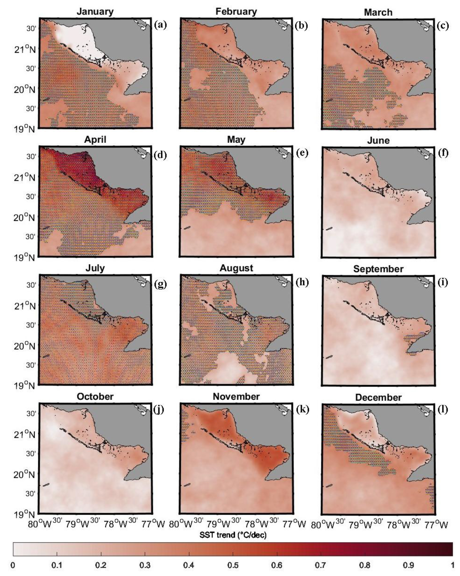
Figure 6 Monthly SST trends (2003–2022). Linear trends of monthly SST anomalies (°C per decade) for January–December (a–l). Trends are estimated by ordinary least squares applied to monthly anomalies at each grid point. Stippling indicates grid cells that are significant at the 95 % level (two-sided t test), using effective degrees of freedom to account for autocorrelation. Warming intensifies in winter and transition months, with maxima in April and November; land is masked in grey.

Monthly SST anomalies (Fig. 7a and c) show greater variability on the shelf (GAM) than offshore (CS), with standard deviations of 0.61 and 0.41 °C, respectively. Several cold winters marked the first half of the record (for example, 2004, 2009, 2011), which were more pronounced in GAM. An additional cold event in 2010 was evident in GAM but weak/absent in CS. In the second decade of study, warm winters predominated (for example, 2014, 2016, 2019, 2020), with stronger occurrences over GAM. Despite not every year conforming to the general trend, results demonstrate an overall evolution that is shifting from predominantly cool to predominantly warm conditions.

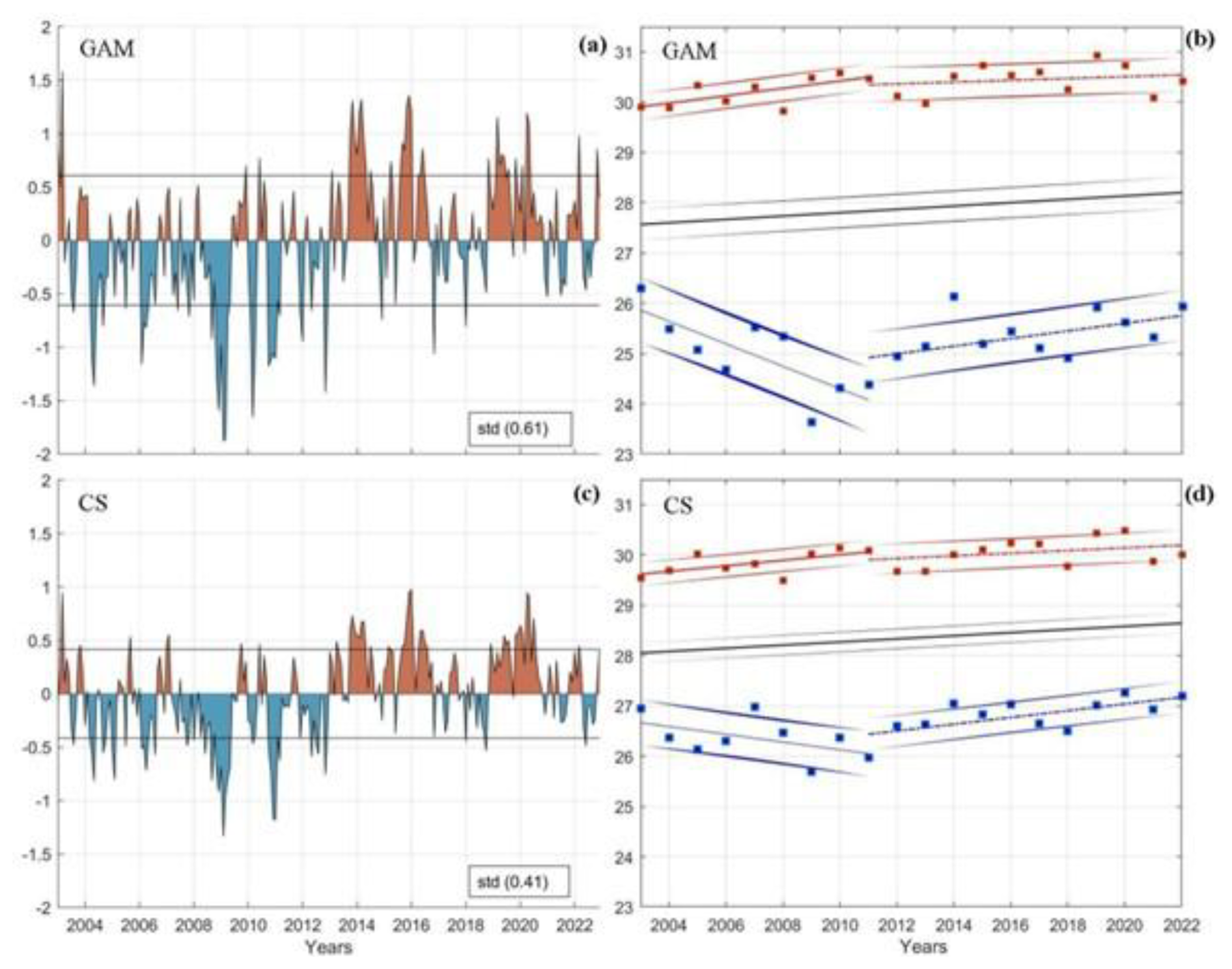
Figure 7 (a, c) Monthly SST anomalies (°C) for the Gulf of Ana María (GAM) and the Caribbean Sea (CS), respectively, 2003–2022. Thin horizontal black lines indicate ±1 SD (standard deviation) over the full period (value shown in each panel). (b, d) Yearly seasonal means for summer (July–August–September; red squares) and winter (January–February–March; blue squares) in GAM and CS, respectively. Black lines show linear trends of the annual means. Coloured lines show piecewise linear fits to the seasonal means prior to (2003–2011) and after (2012–2022) the 2011 transition. All series represent area averages over the GAM and CS boxes shown in Fig. 1a and b.

Seasonal means by year (Fig. 7b and d) confirm that winter (January to March) drives most of the low-frequency change. Piecewise linear fits prior to and after 2011 indicate a winter cooling tendency during 2003–2011, followed by a marked winter warming during 2012–2022. Summer (July to September) warmed throughout the record, albeit with smaller slopes than winter in both regions. The black line in Fig. 7b and d shows the yearly linear trend, which is positive for both GAM and CS. In conjunction, these patterns indicate a step-like transition from 2011 to 2013 to a persistently warmer state, which is coherent across both shelf and offshore boxes. To formally assess whether the apparent transition toward a warmer state is statistically significant, we applied a changepoint test based on a two-phase regression with a common trend (XLW), which is designed to detect a step-like shift in the mean level while allowing for an underlying linear trend. The test was performed on the monthly SST anomaly series for the two representative subregions (GAM and CS; Fig. 7a and c), scanning all admissible changepoint times and using the maximum F statistic (F_max; see Reeves et al., 2007); significance was estimated via Monte Carlo simulation under the null with serial autocorrelation accounted for in the residual structure. The analysis identifies an optimal changepoint in December 2012 in both subregions, consistent with the step-like transition highlighted visually in Fig. 7b and d. The estimated mean-level increase after the changepoint is 0.67 °C for CS (F_max=53.45; 98 % confidence) and 0.84 °C for GAM (F_max=35.75; 95 % confidence). These results provide quantitative support that the late-2012 shift represents a statistically significant transition toward persistently warmer conditions in both shelf and offshore environments.

In summary, the shelf exhibits larger variance and a stronger wintertime response than the adjacent CS, consistent with Sect. 3.1 (shallower mixed layers and stronger air–sea coupling). This transition foreshadows the increase in marine heatwave activity (see below Sect. 3.3) and is consistent with the low-frequency modulation captured by the EOF analysis (Sect. 3.4).

3.3 Marine heatwaves

Spatially, the mean of event-wise maximum intensity ranges from ∼1–2 °C across the domain (Fig. 8a), with a regional mean of 1.3±0.2 °C. Intensities were systematically higher inside the gulf than offshore. Events in GAM tended to have higher absolute intensity, whereas the CS, which experienced lower background variance, more often reached higher MHW categories under the Hobday scheme. The total number of MHW days from 2003 to 2022 exceeds 200 at every grid cell and surpasses 400 over most of the GAM (Fig. 8b).

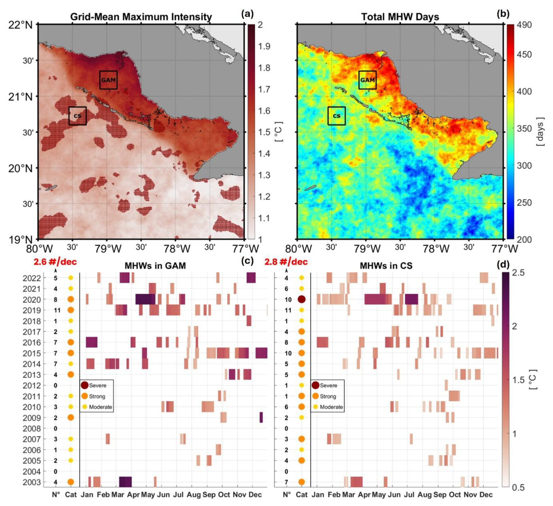
Figure 8 Marine heatwave (MHW) characteristics between 2003–2022. (a) Mean of event-wise maximum intensity (°C) at each grid point. Grid cells that experienced Severe category events at least once are shaded (reddish shading). (b) Total MHW days per grid point accumulated from 2003 to 2022. Black boxes mark the GAM and CS sub-regions. (c, d) Event calendars for GAM and CS, respectively: coloured rectangles denote individual events by month, with darker shading indicating increased intensity (°C). Left-hand columns indicate, for each year, the number of events (No.) and the maximum category reached (circle colour: Moderate/Strong/Severe). At the top left of (c, d), the trend in event frequency is shown as the number of events per decade (# per decade).

The year-by-year event calendars for the representative boxes (Fig. 8c and d) show broadly similar annual frequencies in GAM and CS (typically 4–5 events per year), with a marked increase in frequency and intensity during the second decade. The most active period is 2019–2020, followed by 2015–2016, in both regions. The years 2004 and 2008 are the only ones in which no MHW was detected in either box. Accordingly, a key shelf–offshore contrast emerges: Events in GAM tended to be more intense, while more high-category events were registered in the CS; over the entire period, 73 events were recorded in GAM compared to 90 in CS. These patterns are consistent with the seasonal contrasts established in Sect. 3.1, i.e., shallow, strongly forced shelf waters favour larger absolute temperature anomalies (higher intensity), while offshore, the background threshold and variance regime support more frequent escalation to higher categories.

3.4 Modes of variability

EOFs of monthly SST anomalies (2003–2022) indicate that the first two modes account for 93.7 % of the total variance (EOF1: 87.5 %, EOF2: 6.2 %) and possess clear physical significance (Fig. 9). EOF1 displays a monopole pattern with positive loadings across the domain, slightly enhanced toward the shelf edge and offshore. This mode represents coherent warming/cooling of the entire region. Its principal component (PC1) exhibits low-frequency variability with a pronounced minimum during the 2009–2011 period and positive excursions in the 2013–2016 and 2019–2020 periods. The 2-year low-pass PC1 highlights the step-like transition to a warmer state after the 2011–2013 period, consistent with Sect. 3.2 and with the increase in MHW activity (Sect. 3.3).

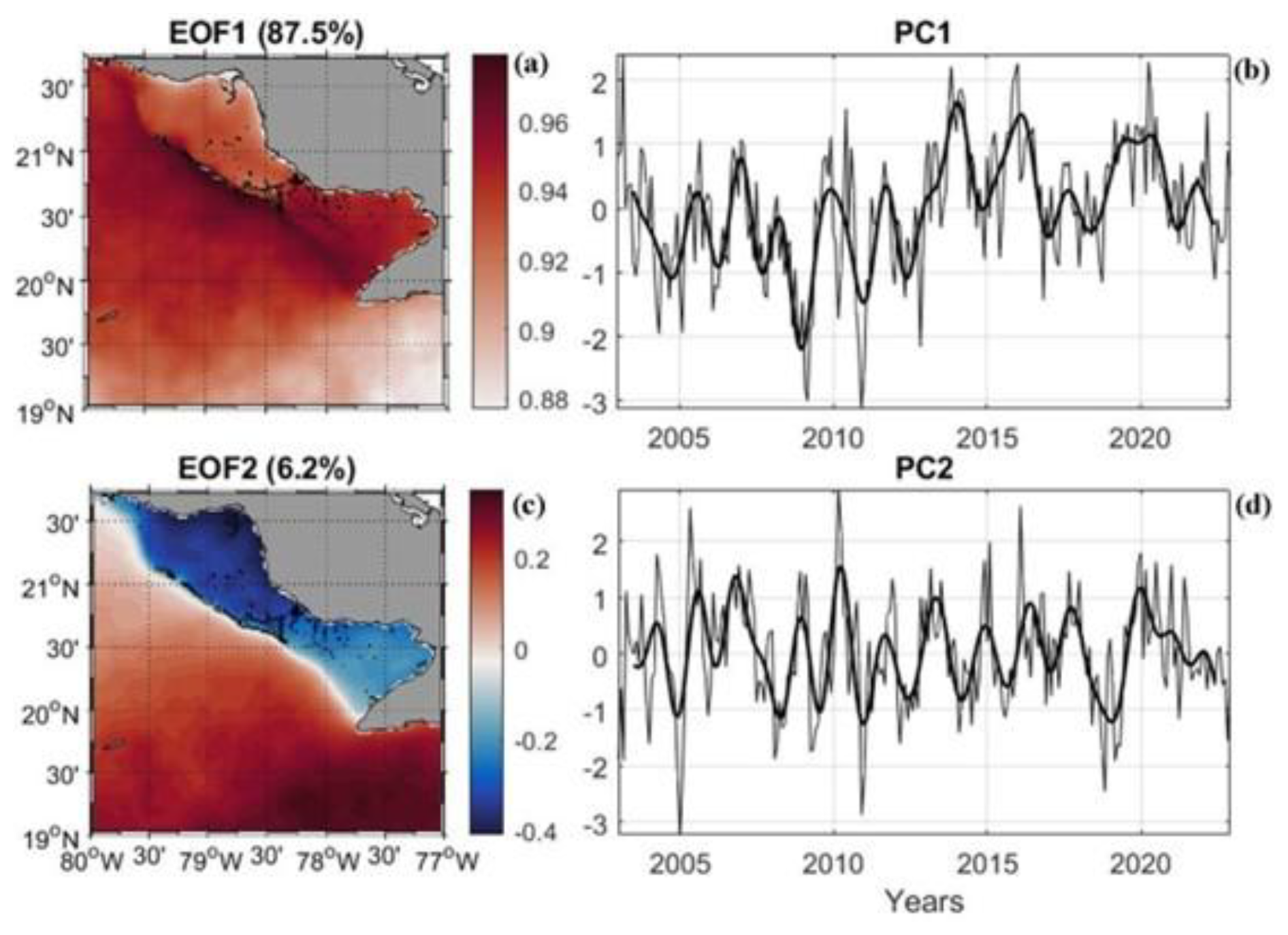
Figure 9 EOF analysis of monthly SST anomalies for 2003–2022. (a, c) Spatial patterns of EOF1 (87.5 %) and EOF2 (6.2 %). (b, d) Corresponding principal components (PC1, PC2); thick black curve represents a two-year low-pass filter to emphasize interannual variability. (PC signs are arbitrary and chosen so that positive PCs correspond to warm anomalies in EOF1.)

EOF2 is a dipole that opposes the shallow shelf (GAM/GG) to the adjacent CS, with larger amplitudes along the shelf break. This mode captures differential heating/cooling between coastal and oceanic waters, consistent with the seasonal mechanisms diagnosed in Sect. 3.1 (stronger air–sea coupling over the shelf and modulation by horizontal advection). PC2 fluctuates primarily at interannual timescales, exhibiting alternating positive/negative phases throughout the period of study, with no persistent trend identified. This indicates variability that redistributes anomalies between the shelf and offshore regions, rather than warming the entire region.

Overall, EOF1 reflects basin-wide anomalies that underpin the regime shift, whereas EOF2 explains spatial structure related to the shelf–offshore gradient. In Sect. 3.5, these modes are related to large-scale climate indices in order to assess likely drivers of the interannual–decadal variability.

3.5 Climate drivers: EOF PCs vs. large-scale indices

A relationship was established between the leading SST modes and climate variability by comparing PC1/PC2 with standard indices (ENSO [MEI], WHWP, TNA and NAO, Sect. 2.4) and with domain-mean latent heat flux (LHF, ERA5). Interannual variability was isolated with a 2-year running-mean low-pass, and low-frequency variability with a 5-year running-mean low-pass (zero-lag correlations reported; significance assessed with effective degrees of freedom; Sect. 2.5).

At interannual scales (Fig. 10a), PC1 co-varies with MEI (r≈0.49), WHWP (r≈0.58), and especially with LHF (r≈0.73), consistent with an air–sea heat-flux pathway linking climate modes to regional SST. At low frequencies (Fig. 10c), PC1 closely tracks the NAO (r≈0.90), consistent with the step-like warming observed after 2011–2013 (Sect. 3.2). The effective degrees of freedom (N^*) and associated significance levels for all correlations (computed after low-pass filtering) are summarized in Table S3.

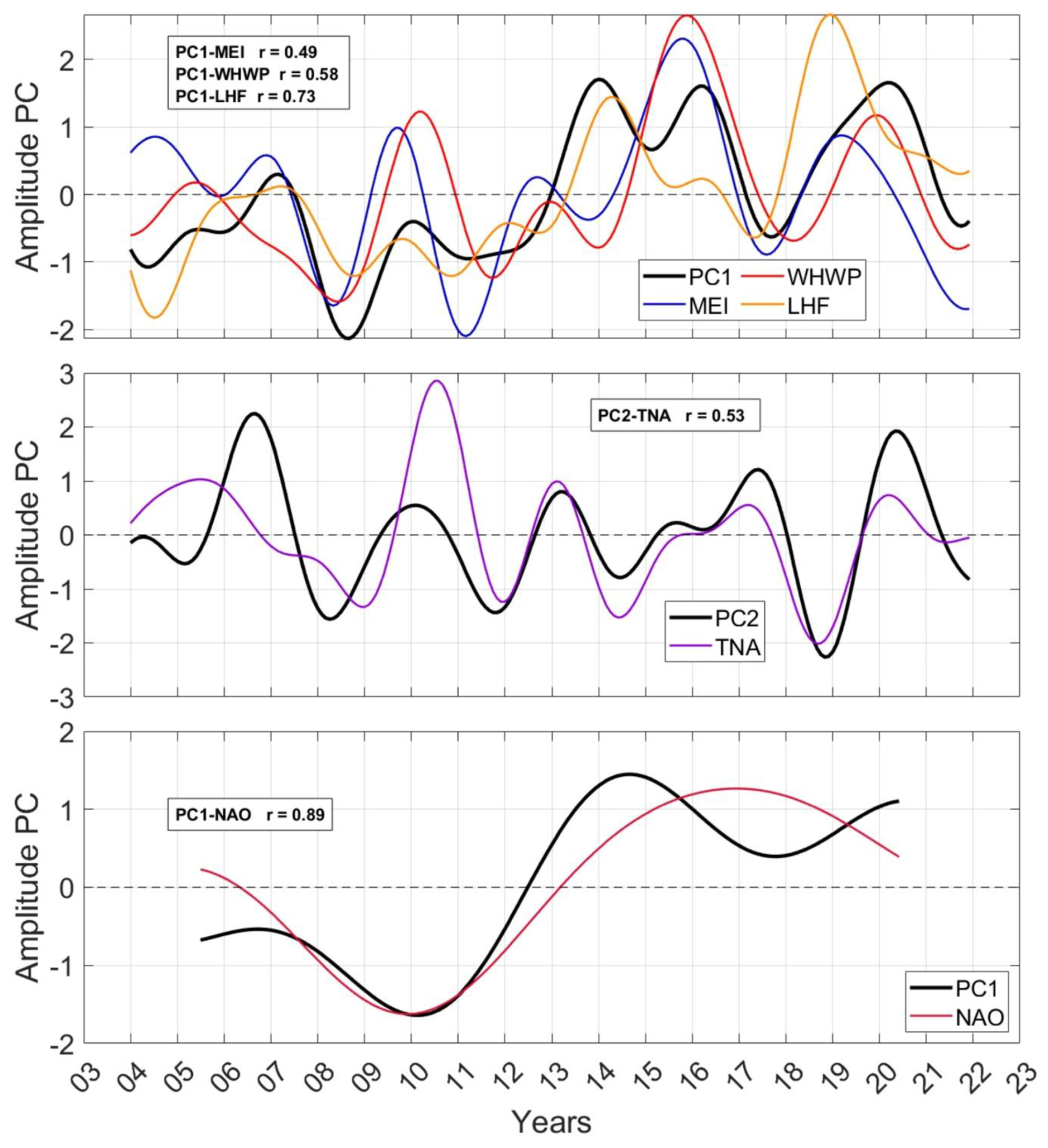
Figure 10 Co-variability of SST principal components (PCs) with climate drivers. (a) Interannual band: 2-year running-mean low-pass of PC1 (black) plotted with MEI.v2 (blue), Western Hemisphere Warm Pool (WHWP) (red), and domain-mean latent heat flux (LHF) from ERA5 (orange). (b) Interannual band: PC2 (black) with Tropical North Atlantic (TNA) (magenta). (c) Low-frequency band: 5-year running-mean low-pass of PC1 (black) with North Atlantic Oscillation (NAO) (red). Numbers in text boxes denote zero-lag Pearson correlations (r) computed on the filtered monthly series. Significance is evaluated using effective degrees of freedom (Sect. 2.5). Series are standardized.

At interannual scales (Fig. 10b), PC2 correlates with the TNA index (r≈0.53), consistent with variability that redistributes anomalies between shelf and offshore rather than producing basin-wide warming. In conjunction, these results indicate that ENSO/WHWP modulates basin-wide anomalies (PC1) via latent heat flux on interannual scales and through the NAO on low-frequency scales. Simultaneously, the shelf–offshore contrast (PC2) is tied to TNA-related variability. Physical mechanisms are discussed in Sect. 4.

4 Discussion

4.1 Seasonal and low-frequency drivers of SST variability

The seasonal evolution of SST in and around JRNP is primarily controlled, with net air–sea heat exchange setting both the sign and timing of the mixed-layer temperature tendency, and horizontal advection providing a secondary modulation near the shelf break. This behaviour is consistent with mixed-layer heat-budget theory, in which surface fluxes dominate the seasonal cycle and heat storage produces an intrinsic lag between forcing and response (de Boyer Montégut et al., 2004; Moisan and Niiler, 1998). The pronounced autumn–winter shelf–offshore contrast arises naturally from mixed-layer-depth differences: for comparable surface forcing, the shallow mixed layer inside the Gulf of Ana María yields larger temperature tendencies ($\propto Q_{\mathrm{net}}/h$), thereby producing faster cooling and stronger gradients than in the adjacent Caribbean Sea. The observed persistence of frontal structures aligned with the shelf edge supports a regime in which thermodynamic forcing establishes the large-scale seasonal baseline, while circulation refine the spatial structure. This interpretation is coherent with prior descriptions of SST variability around Cuba and the southern Cuban shelves, where shelf-ocean contrasts and regional exchange with the Caribbean Sea shape the spatial pattern of SST (González-De Zayas et al., 2022; Caravaca et al., 2022; Cerdeira-Estrada et al., 2005).

Superimposed on this seasonal baseline, the dominant interannual-decadal signal is captured by a coherent basin-wide mode (EOF1) that covaries with ENSO/WHWP and, most directly, with latent-heat-flux variability. This is physically consistent with established Caribbean air–sea coupling pathways, whereby ENSO-related atmospheric anomalies modulate trade winds and near-surface humidity over the warm-pool region, altering evaporative cooling and thus SST at interannual time scales (Wang et al., 2006; Enfield and Lee, 2005; Wang and Enfield, 2001, 2003; Czaja et al., 2002;). In this framework, latent heat flux acts as an efficient bridge between large-scale atmospheric variability and local SST anomalies: weaker trades and/or reduced air-sea humidity gradients reduce evaporation, thereby decreasing upward latent-heat loss and favouring SST warming. The strong co-variability between PC1 and latent heat flux in our results is consistent with this pathway and supports an interpretation in which basin-wide SST anomalies are primarily atmospherically forced through surface turbulent fluxes.

This mechanistic perspective also provides a coherent explanation for the step-like transition toward a persistently warmer state during 2011–2013. The transition is spatially coherent across both, the shelf and offshore subregions and projects strongly onto EOF1/PC1, indicating that it reflects a regional scale forcing rather than a local artefact of subregion selection. At low frequencies, PC1 closely tracks the NAO, suggesting that Atlantic-scale atmospheric variability modulates the background state of surface forcing over the Intra-American Seas (Cook and Vizy, 2010; Wang et al., 2007; Hurrell, 1995). We therefore interpret the 2011–2013 shift as the manifestation of a low-frequency change in atmospheric conditions, which is consistent with NAO-related variability, that favours reduced net surface heat loss (through changes in winds and turbulent fluxes), allowing heat to accumulate and the system to transition into a warmer mean state. This interpretation is further supported by the timing of the transition in the low-pass PC1 and its correspondence with the increase in MHW activity during the second decade of the record. While the present analysis cannot establish causality, the proposed mechanism is physically grounded and consistent with the documented influence of ENSO/WHWP and Atlantic variability on Caribbean air-sea coupling and evaporative cooling (Cook and Vizy, 2010; Wang et al., 2006, 2007; Enfield and Lee, 2005; Wang and Enfield, 2001, 2003; Czaja et al., 2002; Hurrell, 1995).

Finally, the secondary mode (EOF2) helps interpret how large-scale variability translates into spatial structure at local scales. Its shelf–offshore dipole and relationship with the Tropical North Atlantic index indicate variability that redistributes anomalies between the semi-enclosed gulfs and the adjacent open Caribbean Sea rather than warming the entire region uniformly. Physically, such redistribution is consistent with differential mixed-layer coupling and with the role of horizontal gradients and shelf-break dynamics in shaping SST patterns. Importantly for JRNP, this multi-scale framework implies that MHW risk is conditioned by (i) the local thermodynamic sensitivity of shallow shelf waters to surface forcing and (ii) large-scale atmospheric variability that favours persistent warm anomalies, both of which are relevant for coral-reef thermal stress and associated ecological impacts (Cramer et al., 2020; Bruno et al., 2019; van Hooidonk et al., 2015; Hughes et al., 2003). From an applied perspective, these results support monitoring surface heat fluxes and mixed-layer depth alongside large-scale indices (ENSO/WHWP and NAO) to provide a physically informed context for early-warning assessments in the JRNP under continued warming.

4.2 Marine heatwaves: intensity, category and recent escalation

Marine heatwaves increased in frequency and intensity during the second decade, with 2019–2020 being the most active period, followed by 2015–2016 as the second most active. MHW detection and categorization follow Hobday et al. (2016, 2018). Relative to the local 90th-percentile threshold, the mean of event-wise maximum intensity is greater in GAM than offshore, while the total number of MHW days surpasses 400 across large areas of the gulf. However, the higher category scales (for example, Severe) occur comparatively more often offshore (CS). This contrast is expected under the Hobday scheme, in which categories are defined by the magnitude of local threshold exceedance. Thus, regions with lower background variance can experience higher categories, even for more minor absolute anomalies. Physically, GAM develops larger °C anomalies due to shallow, strongly forced mixed layers, while CS more readily crosses category thresholds owing to tighter local variability.

The warmer background state after the 2011–2013 period effectively preconditions the region for MHW development, increasing both the likelihood and persistence of threshold exceedances. Mechanistically, this links back to Sect. 3.1 and 3.5, whereby flux-dominated seasonality sets the baseline and phase, and large-scale atmospheric variability modulates the probability of sustained warm anomalies that seed or prolong events. These patterns echo broader reef-climate concerns in the Caribbean, where rising SSTs and compounding stressors have been associated with bleaching and ecological change (Hughes et al., 2003; Bruno et al., 2019; Cramer et al., 2020; van Hooidonk et al., 2015), including at JRNP and neighbouring MPAs (Pina-Amargós et al., 2008; Hernández-Fernández et al., 2011, 2016, 2019; Gerhartz-Muro et al., 2018; Caballero-Aragón et al., 2020).

4.3 Limitations, assumptions and robustness

Several methodological choices bound the interpretation. The budget is formulated for the bulk mixed layer and, as a consequence, we used GLORYS12 mixed-layer temperature, depth and currents for internal consistency among terms, by computing all tendencies on a daily basis and averaging these to monthly values. MUR SST was reserved for descriptive and MHW analyses. At monthly scales, MLT and SST are well correlated; however, residual differences may persist at daily scales due to skin effects and diurnal warming.

ERA5 and GLORYS12 may exhibit coastal biases. Particularly, it was not possible to directly evaluate the realism of GLORYS12 currents in the gulfs or the adjacent CS because no in-situ velocity observations (for example, those undertaken by Acoustic Doppler Current Profiler moorings or high-frequency radars) were available for the study period. This is a non-trivial caveat: reproducing circulation in highly shallow, embayed shelves, such as the GAM and the GG, is notoriously challenging for global reanalyses. This is because the effective 1/12° (∼8–9 km) resolution and required bathymetric smoothing under-resolve narrow channels, weak pressure-gradient flows and small eddies. Moreover, the abrupt depth changes along the shelf break and the roughness and enhanced bottom friction associated with coral-reef frameworks further challenge the representation by the model of nearshore dynamics. Accordingly, the advective term in the mixed-layer budget herein should be interpreted as a conservative lower bound, which captures sign and seasonality but, potentially, underestimates magnitudes close to the coast. Targeted in-situ current measurements and/or nested higher-resolution regional modelling would help refine the role of advection within the gulfs.

Trends and correlations account for serial autocorrelation through effective degrees of freedom. EOFs were analyzed from raw data as well as from data to which 2 and 5 year low-pass filters were applied. While filtering choices can shift correlation maxima to a certain degree, they do not alter the physical interpretation. The 1 km MUR record dictates the 20-year baseline (2003–2022) and is shorter than the canonical 30-year climatology. Thresholds and category counts may therefore be modestly sensitive to baseline choice; extending thresholds with longer-record products (for example, coarser-resolution SST) would represent a more thorough sensitivity check.

Overall, such limitations do not alter the headline result: that surface heat flux dominates the seasonal cycle, that basin-wide anomalies are atmospherically forced, and that shelf–offshore contrasts arise from the interplay of mixed-layer depth and horizontal gradients.

4.4 Implications for JRNP and outlook

Two immediate implications follow. First, the strong coupling between net heat flux and temperature, in conjunction with the typical ∼2 month lag, suggest that simple seasonal outlooks based on forecasts of radiative and turbulent fluxes and mixed-layer depth could offer early warning of forthcoming warming or cooling within GAM. Second, routine tracking of ENSO/WHWP (interannual) and NAO (low-frequency) provides a large-scale context for risk assessment. Consequently, positive phases aligned with reduced latent-heat loss increase the likelihood of basin-wide warmth (PC1) and, consequently, of MHW occurrence and persistence.

Moving forward, the following aspects have the potential to directly contribute to improving knowledge and forecasting capacity in the region: (a) in-situ observation of currents and conductivity, temperature and depth (from moorings or gliders transects) within JRNP and across the shelf break; (b) extended MHW climatologies, for example, by deriving thresholds from longer-record SST products, while retaining MUR for spatial detail; (c) targeted analyses of regional circulation features, such as shelf-break jets or eddy interactions, that may enhance advection during transition seasons at the local level; and (d) a practical next step is to implement a regional, high-resolution ocean model (for example, CROCO) nested in GLORYS12/ERA5 and tailored to the JRNP–GAM–GG system. A horizontal resolution of ∼1 km or finer (with tidal forcing, realistic bathymetry/reef roughness and bulk fluxes) would enhance efforts to resolve shelf-break jets, gulf exchanges and frontal dynamics that are under-represented in global reanalyses. Such steps would not only consolidate the mechanistic framework presented herein, but also help to translate it into operational guidance for conservation and management within the national park.

5 Conclusions

The present study has quantified seasonal-to-decadal variability of sea-surface temperature in and around the Jardines de la Reina National Park, with the primary objective to identify the mechanisms and climate drivers that shape this variability, using daily 1 km MUR SST (2003–2022), ERA5 surface fluxes and GLORYS12 mixed-layer fields.

A mixed-layer heat budget shows that net surface heat flux sets the seasonal evolution of SST, with horizontal advection providing a smaller modulation near the shelf break; a characteristic ∼2-month lead of flux over temperature is consistent with mixed-layer heat storage and explains the enhanced winter cooling and stronger thermal gradients along the shelf edge. A clear shelf–offshore contrast emerges: the shallow gulfs (GAM/GG) markedly differ from the adjacent Caribbean Sea in autumn–winter (November–March), whereas conditions during spring–summer are comparatively homogeneous. This reflects shallower mixed layers and greater flux sensitivity inside the gulfs, with advection adding local modulation. Superimposed on this baseline is a warming trend of ∼0.28 °C per decade (2003–2022), which is strongest in winter and transition months, with monthly maxima around April (∼0.48 °C per decade) and November (∼0.35 °C per decade), and a step-like transition in 2011–2013 towards a persistently warmer state. The warming trend is predominantly driven by the phase shift of the NAO, since the study period begins in a negative phase and ends in a positive phase. In addition, the interannual to decadal modulation of other dominant climatic oscillations in the region (ENSO, WHWP), in conjunction with latent heat fluxes, favours the progressive accumulation of heat in the ocean surface layer.

Marine heatwaves intensified during the second decade (with the 2019–2020 period the most active, followed by 2015–2016). Mean event-wise maximum intensity is higher within GAM, whereas upper categories occur relatively more often offshore, consistent with lower background variance in the area, while total MHW days exceed 200 across the domain and 400 over much of the gulf. EOFs separate a basin-wide mode (EOF1, 87.5 %), co-varying interannually with ENSO/WHWP and latent-heat flux and at low frequencies with the NAO, from a shelf–offshore dipole (EOF2, 6.2 %) linked most clearly to TNA. This indicates atmospheric forcing of basin-wide anomalies with regional thermodynamics and advection setting spatial structure.

Practically, seasonal outlooks based on forecasts of net heat flux and mixed-layer depth, in addition to routine monitoring of ENSO/WHWP and NAO, can help to inform MHW risk in relation to JRNP. Indeed, a regional high-resolution ocean model (for example, ROMS/CROCO at ∼1 km or finer), combined with targeted in-situ observations, would further improve prediction and attribution. In conjunction, the results of the present research provide a physically grounded baseline for anticipating future thermal stress and for guiding conservation and management efforts within JRNP in response to continued climate warming.