A novel multispecies approach for the detection of regime shifts in a plankton community – a case study in the North Sea

The physical environment both above and below the ocean surface has changed dramatically during the last century. Changes in the marine environment induced by increased release of greenhouse gases and direct exploitation of resources include increased ocean temperature, decreased salinity and pH, and removal of apex predators. The risk of ecological regime shifts occurring has similarly increased. A variety of methodologies to identify regime shifts have already been used in the North Sea, which has become an important case study for the analysis of regime shifts in a semi-enclosed waterbody. The North Sea is regarded as a case study in part due to the operation of the continuous plankton recorder, which has provided detailed abundance records of phyto- and zooplankton for over 60 years. Here, we propose a new methodology to calculate regime shift likelihood for every month between 1958 and 2020. This unique model produces a single time series of regime shift likelihood, using sequential abundance data of more than 300 plankton species. We show the model's ability to identify when regime shifts occurred in the past by comparing it to previous less automated methodologies. We have validated the model for use in the North Sea by estimating how often false positives and false negatives are generated. Results from the model indicate evidence for three periods of high regime shift likelihood in various parts of the North Sea: between 1962 and 1972, between 1989 and 1999, and from 2002 until 2015. We show that these periods are consistent with previous estimates of North Sea regime shifts, and discuss possible applications of the model's output of a single time series.

1 Introduction

The global ocean plays a critical role in regulating climate on Earth through heat and carbon redistribution. Global mean ocean temperature has increased since the Industrial Revolution, potentially inducing extreme events (IPCC, 2019). Changes in the oceanic environment associated with long-term temperature increase include more frequent marine heatwaves (Oliver et al., 2018, 2019), decreased pH (Doney et al., 2009), loss of oxygen concentration (Heinze et al., 2021; IPCC, 2019), and changes to large-scale circulation patterns such as the Atlantic Meridional Overturning Circulation (AMOC) (Johnson et al., 2020; Robson et al., 2014), salinity (Curry et al., 2009; Skliris et al., 2014), and stratification stability in the upper ocean (Hallegraeff, 2010; Sharples et al., 2006; Wells et al., 2020). The projected rates of ocean warming, acidification, and oxygen concentration are strongly dependent on the rate of greenhouse gas emissions (Kwiatkowski et al., 2020; Schmidtko et al., 2017). In 2017, signatories to the Paris Climate Agreement agreed therefore to limit global temperature increase to less than 2 °C by the end of the 21st century (Fox-Kemper et al., 2021). At current emission rates, it is likely that we will exceed these limits by 2050 (Fox-Kemper et al., 2021), which will potentially lead to the crossing of planetary boundaries, tipping points, and ecological regime shifts (Heinze et al., 2021; Rocha, 2022).

Regime shifts are characterized by large, abrupt, and persistent changes in the function and structure of an ecosystem that are not easily reversible (Scheffer et al., 2001; Reid et al., 2016). Such reorganizations of the ecological system can be, but are not always, preceded by dynamics such as critical slowing down (Scheffer et al., 2001; Scheffer, 2009; Wouters et al., 2015). Regime shifts preceded by critical slowing down are associated with an erosion of dominant feedback mechanisms until a critical threshold, the so-called tipping point, is crossed (Biggs et al., 2018). Regime shifts are ecologically important, in part due to the possible presence of hysteresis or non-reversibility of changes (Sguotti et al., 2022). In open ocean systems regime shifts are notoriously difficult to identify (Haines et al., 2024; Rudnick and Davis, 2003; Beaugrand, 2004b; Scheffer et al., 2001), because statistically significant estimates of biodiversity changes require sufficiently long time series. For example, it is thought that at least 50 years of measurements are needed to detect ecological changes driven by changing climate conditions, including regime shifts (Edwards et al., 2010), though there are studies which have used a shorter time frame (Hare and Mantua, 2000). Regime shifts in marine systems have therefore been documented most often in regions where in situ measurements and remote sensing data are relatively abundant, such as the northeast Pacific Ocean (Hare and Mantua, 2000), along the Norwegian coast (Vollset et al., 2022), and the North Sea (Beaugrand, 2014; Djeghri et al., 2023; Beaugrand and Reid, 2003; Edwards et al., 2001; Sguotti et al., 2022). In fact, the North Sea has become a case study for detecting regime shifts in marine environments. The North Sea has undergone monitoring by the continuous plankton recorder (CPR), which constitutes one of the longest marine ecological time series, and diligent fishery records. Despite this, considerable controversy remains around the identification of regime shifts.

Abrupt changes in the abundance of a single species may be indicative of either a regime shift, which may be seen in multispecies communities and ecosystems, or representations of decadal variability. Different regime shift identification methods are often applied to ecological or physical systems, but autocorrelation and critical slowing down signals have been detected in both systems (Overland et al., 2006; Scheffer et al., 2001; Rudnick and Davis, 2003; Haines et al., 2024). In order to differentiate the presence of multiple climatic stable states from multidecadal fluctuations, Overland et al. (2006) applied different statistical signals, including white and red noise, to the context of regime shift identification. Classical detection methods have been shown to falsely identify regime shifts in simulated time series data of species abundance, to which red noise had been introduced (Haines et al., 2024; Rudnick and Davis, 2003). A correct and simple identification of regime shifts is crucial for future management of ecosystems. Previous studies have often focused on periods where specific species experienced an abrupt shift (Alvarez-Fernandez et al., 2012; Beaugrand, 2014; Djeghri et al., 2023; Reid et al., 2001; Vollset et al., 2022), which can be identified using split moving window boundary analysis (Alvarez-Fernandez et al., 2012; Beaugrand, 2014) or change-point analysis algorithms (Boulton and Lenton, 2019; Arellano-Nava et al., 2022).

In our study, we apply a specific change-point analysis algorithm to a group of species at once, in order to create a single time series of regime shift likelihood. Producing a single time series of regime shift likelihood must necessarily remove context. This is a major difference from previous methods like the split moving window boundary analysis (Alvarez-Fernandez et al., 2012; Beaugrand, 2014) or exploration of principle component analysis (Djeghri et al., 2023), which are concerned with indicating which species or functional groups were changed with apparent regime shifts. An advantage of new approach over previous methods is that construction of a single time series of regime shift likelihood can be the first step towards exploring potential drivers through linear analysis.

Knowledge of ecosystems requires reliable time series from preferably more than one trophic level, for as many years as possible (Edwards et al., 2010; Wouters et al., 2015). Regime shifts in plankton are often detected in higher trophic levels first despite signals possibly previously being present in lower trophic levels (Reid et al., 2001; Vollset et al., 2022; Beaugrand, 2014). More data from higher trophic levels can be used to identify whether a system is controlled from the bottom up or through other means (Di Pane et al., 2022; Fauchald et al., 2011). Due to their relatively short lifespans and rapid generation time, planktonic organisms are especially useful for studying ecological responses to changing conditions in both the recent (Bowler et al., 2010; Beaugrand, 2004b; Djeghri et al., 2023) and ancient past (Strack et al., 2022; Lowery et al., 2020). The idea of using plankton as a “canary in the coal mine” to provide early warnings of wider regime shifts is not unique (Bowler et al., 2010). For example, it has been well documented using CPR data that a regime shift occurred in the North Sea between the years of approximately 1982 and 1988, evidenced by the sudden change in abundance of calanoid copepods Calanus finmarchicus and Calanus helgolandicus (Beaugrand and Reid, 2003; Reid et al., 2016, 2001). Some studies have suggested a change in the plankton community impacted higher trophic levels or ecosystem function, but not all agree (Djeghri et al., 2023; Reid et al., 2001).

In our study, we have analyzed multiple time series of plankton abundance simultaneously. We here describe the process of generating a single time series representing the likelihood of a regime shift occurring at any point represented by the time series. The aim of designing a new automated methodology for detecting regime shifts was not simply to add to the growing list of statistical methods and models already in use (see Alvarez-Fernandez et al., 2012; Beaugrand et al., 2014; Djeghri et al., 2023; Haines et al., 2024). The method described here does not require the user to identify particular species of interest before analyzing a dataset but rather uses all species in a dataset to estimate the likelihood of a regime shift occurring. Figures can be made showing the time series of species abundance with the greatest difference in abundance over time and which therefore likely contributed most to regime shift probability being high. These features are particularly valuable if the planktonic ecological history of the study area is not well known. We applied the new regime shift identification method to four areas of the North Sea. The method indicated regime shifts during periods and showed causative species were likely consistent with those found by previous methods. We discuss advantages and limitations of the new method, as well as possible future uses.

2 Methods

2.1 Study area

The study area is comprised of the marine environment within 50 and 65° N and 10° W and 8° E (Fig. 1). Using CPR sampling areas (also utilized by Montero et al., 2021; Alvarez-Fernandez et al., 2012; Djeghri et al., 2023) to search for evidence of regime shifts has been done previously and allows for the results of our approach to be compared to other previous results.

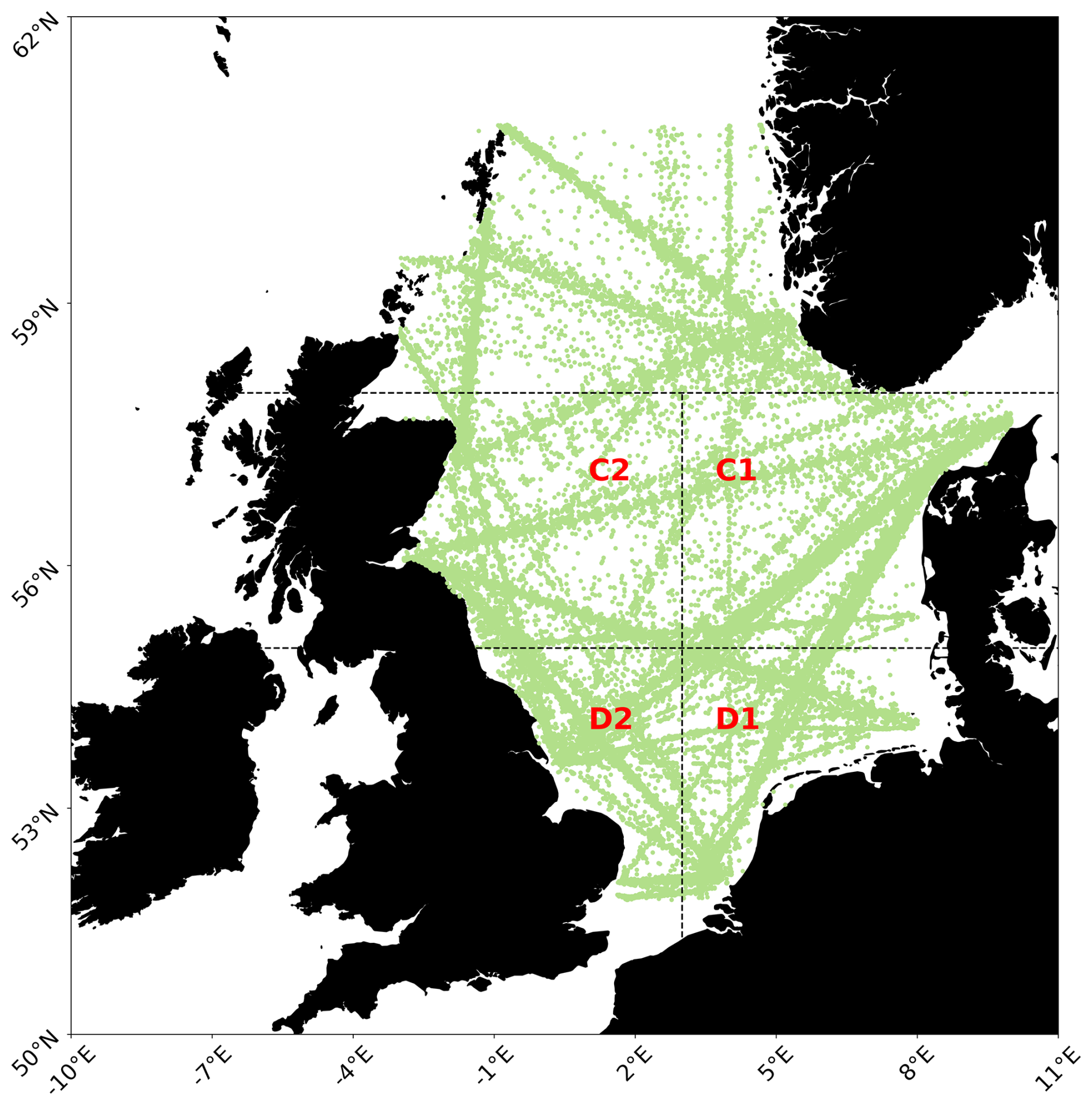
Figure 1 The North Sea study area with sampling points displayed in green, and CPR areas C1, C2, D1 and D2 denoted by dashed lines and area names in red. Map was built using Elson et al. (2024).

2.2 Ecological data

Abundance data concerning phytoplankton and zooplankton from 1958 until 2019 were obtained from the CPR (see Reid et al., 2003 for detailed methodology). Abundance data from the CPR for the over 200 phytoplankton species and 80 zooplankton species are given in captured organisms per 18 520 m (equivalent to 10 nautical miles) of towing (Reid et al., 2003). Removing the seasonality trends of these data was accomplished by converting abundances into monthly anomalies for each year using Eqs. (1) and (2).

Because the CPR survey is conducted by ships of opportunity, data from the CPR are highly variable in spatial and temporal resolution (Reid et al., 2003; Richardson et al., 2006). Sampling devices are towed behind ships at an average depth of 7 m, but this is also variable. There are some groups of plankton which are not routinely collected by the CPR survey, primarily large zooplankton (Marques et al., 2024) and some smaller species of phytoplankton (Richardson et al., 2006; Mengs et al., 2024). However, the distance covered and the period of operation provided by the CPR survey is unmatched by other plankton datasets and is thus a highly valuable source of ecological data (Beaugrand, 2004a; Beaugrand et al., 2014; Djeghri et al., 2023).

The Phytoplankton Color Index (PCI) is a logarithmic graded color scale estimated by the CPR Survey Group, and has been used as a proxy for chlorophyll concentration (Beaugrand, 2014; Reid et al., 2003). The PCI is a color scale completely separate from phytoplankton cells counted per sample, although high cell counts are likely correlated with high PCI. A logarithmic transformation was also applied to phytoplankton and zooplankton species captured by the CPR (Eq. 1), before mean abundance was calculated (Eq. 2):

$$\begin{array}{}\text{(1)}& x^{\prime }={\log }_{\mathrm{10}}\left(x_i+{\displaystyle \frac{\mathrm{LOQ}}{\mathrm{2}}}\right),\end{array}$$

where x is the species abundance as measured by the CPR at time point i and LOQ is the CPR limit of quantification, a constant of 20 cells per 10 nautical mile sample. The logarithmic transformation was applied to reduce the strong seasonal contrasts in abundance, particularly during bloom periods, and to stabilize variance across time series. This approach is commonly used for plankton data, where values can span several orders of magnitude (Djeghri et al., 2023; Beaugrand et al., 2014; Bedford et al., 2020a). Logarithmic transformation necessitates the additional manipulation of adding half the limit of quantification to avoid calculating logs of zero. Changing original data in two ways instead of one, such as in square root transformations, is not ideal, but logarithmic transformations were chosen because of the exponential difference in seasonal range observed in plankton abundance data and due to its use in previous studies (Beaugrand et al., 2014; Dees et al., 2017).

Mean abundance at each time step was calculated using Eq. (2), which also removed the seasonality signal from abundance time series:

$$\begin{array}{}\text{(2)}& \mathrm{\Delta }x\left(t\right)=x\left(t\right)-{\stackrel{\mathrm{‾}}{x}}_m,\end{array}$$

where Δx(t) is the mean abundance anomaly at year-month t which includes every month of every year between 1958 and 2019. x(t) is the mean abundance of each species after the transformation detailed in Eq. (1) has been applied, calculated over time step t. ${\stackrel{\mathrm{‾}}{x}}_m$ represents the mean abundance when the month m is the same as t but calculated over all years.

2.3 Detection and identification of regime shifts

The regime shift detection algorithm implemented here follows the method described by Boulton and Lenton (2019). The method of Boulton and Lenton (2019) was designed for use on detrended data, which required the removal of a seasonal signal from abundance time series (see Eq. 2). Converting raw data into logarithmically transformed anomalous means using Eqs. (1)–(2) is a necessary step before detecting abrupt shifts, as described in the following section. There is a risk that important features of the dataset, such as maxima and minima, are removed with this transformation. This is likely to result in more conservative estimates of abrupt changes in abundance. The largest driving force of plankton abundance throughout the year in temperate oceans is seasonality, but this was not the primary concern of this study. This model may not be suitable for identification of regime shifts exhibiting as changes to phenology or the timing of phytoplankton blooms.

The core idea behind this approach is to detect anomalous rates of change in a time series, based on the premise that regime shifts correspond to unusually steep increases or decreases in the gradient over short periods. The algorithm begins by dividing the time series into fixed-length, non-overlapping segments. Within each segment, a simple linear regression is applied to estimate the slope, representing the local rate of change. These slopes are then compared across all segments. To identify anomalous trends, the algorithm calculates the median slope and the median absolute deviation (MAD). Slopes that deviate from the median by more than three MADs are flagged as anomalous. In this context, linear regression is used solely to quantify rates of change: since no statistical inference is involved, assumptions such as normality and homoscedasticity are not required (Schmidt and Finan, 2018). We adapted and refined the Python version (Arellano-Nava et al., 2022) of this method to estimate the likelihood of a regime shift across multiple species and trophic levels, presenting the results as a single time series. Our approach is referred to as the RST (Regime Shift Time-series) model throughout this paper (Dees, 2025).

To track these anomalies, a regime shift indicator time series is initialized with zeros. At each time step corresponding to the center of an anomalous segment, the indicator is updated with +1 (for a steep positive slope) or −1 (for a steep negative slope). This process is repeated across a range of segment lengths, from a user-defined minimum to a maximum of one-third of the total series length. The cumulative indicator values are then divided by the number of segment lengths used, yielding a continuous regime shift likelihood index ranging from −1 to 1. Values near 0 suggest a low likelihood of abrupt change, while values approaching −1 or 1 indicate a high likelihood of a regime shift, with the sign reflecting the direction of change.

We applied this single-series regime-shift detection algorithm to identify abrupt changes in each species across the entire plankton community from the CPR dataset. The RST model is able to identify abrupt changes when assessing time series with regular time steps. This required the CPR dataset to be converted to a time series of mean anomaly abundances for each month in every year that the CPR has been in operation (see Sect. 2.2). Regime shift likelihood time series were generated for the logarithmically transformed time series of mean abundance per month per year (Δx(t)) and the logarithmically transformed time series of zooplankton abundance anomaly. The resulting time series indicates the likelihood of an abrupt change occurring at each time step for each species of zooplankton and phytoplankton captured by the CPR.

A low-pass filter was applied to abrupt change likelihood time series of each species. Distinct abrupt changes for species were determined by the abrupt shift likelihood exceeding the mean and standard deviation of the entire abrupt change likelihood time series. After an abrupt change was identified, Eq. (3) was used to check if the mean abundance of the species was different after the abrupt shift:

$$\begin{array}{}\text{(3)}& -\mathrm{2}{\mathit{\sigma }}_A<({\stackrel{\mathrm{‾}}{x}}_{\mathrm{0}}-{\stackrel{\mathrm{‾}}{x}}_{\mathrm{1}})<\mathrm{2}{\mathit{\sigma }}_A,\end{array}$$

where ${\stackrel{\mathrm{‾}}{x}}_{\mathrm{0}}$ and ${\stackrel{\mathrm{‾}}{x}}_{\mathrm{1}}$ are the mean abundance of species before and after an abrupt change, respectively, as determined by the algorithm of Boulton and Lenton (2019). The low-pass filter removed abrupt changes from the results if the mean abundance before and after a supposed abrupt shift did not differ by at least 2 standard deviations.

Next, we constructed a probability table to estimate the probability of an abrupt change for the entire sampled plankton community at each time point. For each species analyzed, the standard deviation of the regime shift likelihood time series was calculated. We then applied a series of weights to the likelihood of a regime shift occurring at every time step throughout the study period.

A rolling mean with a window length of 24 months was applied to the time series of abrupt shift likelihood, for each species. The length of this rolling window was chosen because changes in the phytoplankton community are assumed to influence the zooplankton community (Capuzzo et al., 2018; Marques et al., 2024), and we assumed that two annual cycles would be long enough to capture this influence. After making this assumption, a series of figures were made to test the effect of iteratively changing the number of months in the rolling window. The code provided here allows the user to explore alternative rolling window lengths, and we encourage future studies to do so (see Supplement).

Weights, based on the duration of sustained anomalies, were added to the relative importance of the time series of the likelihood of abrupt change if the time series exceeded one absolute standard deviation for an extended period (Eq. 4). This meant the added weight grew exponentially for species where standard deviation was exceeded for a longer time over the course of a 24-month rolling window. Sustained deviation away from a beginning point therefore had a greater effect than sudden changes which did not last longer than 5 months:

$$\begin{array}{}\text{(4)}& w=\left\{\begin{array}{ll}\mathrm{1}& \text{if }n<\mathrm{5}\\ \mathrm{2}& \text{if }\mathrm{5}\le n<\mathrm{10}\\ \mathrm{4}& \text{if }\mathrm{10}\le n<\mathrm{20}\\ \mathrm{10}& \text{if }n\ge \mathrm{20}\end{array}\right..\end{array}$$

Here, n is equal to the number of times the probability of an abrupt change was greater than 1 standard deviation away from 0, and w is the weight added to the total probability of a regime shift occurring. Again, the weights added in this study assume bottom-up control of North Sea plankton populations, as found by previous studies (Marques et al., 2024; Capuzzo et al., 2018). Not all plankton populations are bottom-up controlled. Regime shifts may sometimes be caused by removal of predators (Eklöf et al., 2020), and we encourage future studies to explore modifying the weights described here.

These weighted series were then summed across species to generate community-level indices for zooplankton (P_zoo(t)) and phytoplankton (P_phy(t)). The total probability of a regime shift in the plankton community was then calculated by adding the probability of an abrupt change in phytoplankton and zooplankton together.

$$\begin{array}{}\text{(5)}& P_{\text{RS}}\left(t\right)=P_{\text{zoo}}\left(t\right)+\mathrm{2}\sum _{t-\mathrm{23}}^t{P}_{\text{phy}}\left(t\right)\cdot P_{\text{zoo}}\left(t\right)\end{array}$$

Here, P_RS(t) is the total probability of a regime shift in the plankton community at time t, P_zoo(t) is the summed abrupt change likelihood for all zooplankton species at time t, and ${\sum }_{t-\mathrm{23}}^t{P}_{\text{phy}}\left(t\right)$ is the summed abrupt change likelihood for all phytoplankton species between time t and the previous 23 months. The product P_phy(t)⋅P_zoo(t) captures co-occurring abrupt changes in both phytoplankton and zooplankton, reflecting potential bottom-up propagation of regime shifts. Doubling this interaction term emphasizes the influence of phytoplankton variability on zooplankton dynamics within a 24-month window. We reiterate that the relative strength of bottom-up controls (Di Pane et al., 2022) and wasp-waist controls (Fauchald et al., 2011) on zooplankton in the North Sea is debated. However, we here assume a change in phytoplankton could induce sustained changes in zooplankton, which allowed us to quantify P_RS(t).

Adding the chosen weights (Eq. 4), and including results from the previous 24 months of the phytoplankton probability time series means that results from the first 2 years of the RST time series will be inaccurate (see Supplement). We encourage future studies to explore different ways of calculating P_RS(t) and how P_RS(t) changes under greater top-down control.

The time series of regime shift likelihood for all species was then converted into a percentage, so as to force the weighted scores for regime shift likelihood into a comparable estimate. Making RST model output a percentage means the estimated likelihood of a regime shift always reaches 100, even if the pre-percentage likelihood remains relatively low. This is an important limitation of the RST model, and must be taken into account when interpreting output which does not appear to vary for extended periods of time. In order to allow for a degree of uncertainty around the estimated percentage likelihood of a regime shift, the absolute deviation around the mean percentage was also calculated at each time step. The results of this time series were plotted with the PCI, used as a proxy for chlorophyll concentration, and the two most abundant phytoplankton and zooplankton species.

The model code allows the user to choose whether regime shifts are indicated when the percentage change in a regime shift occurring rises above a chosen threshold, or when the rate of change in percentage likelihood increases above a chosen threshold in too short of a time period. In the present study, we opted to indicate possible regime shifts using the critical gradient of 20 %. We here define a critical gradient as the change in percentage likelihood of a regime shift occurring between months. The choice to use a critical gradient to identify regime shifts was made because the percentage likelihood of a regime shift can remain above 50 %–60 % for prolonged periods when abrupt changes are induced in only a small percentage of species (see Fig. 2). Large changes in regime shift likelihood are more indicative of abrupt changes occurring in multiple species simultaneously. We chose to use the critical gradient of 20 % in the present study as validation tests indicated this resulted in an acceptable balance between false positive and false negative rates (Fig. 8). The limitation of the RST model producing time series that always reach 100 % has thus been mitigated somewhat.

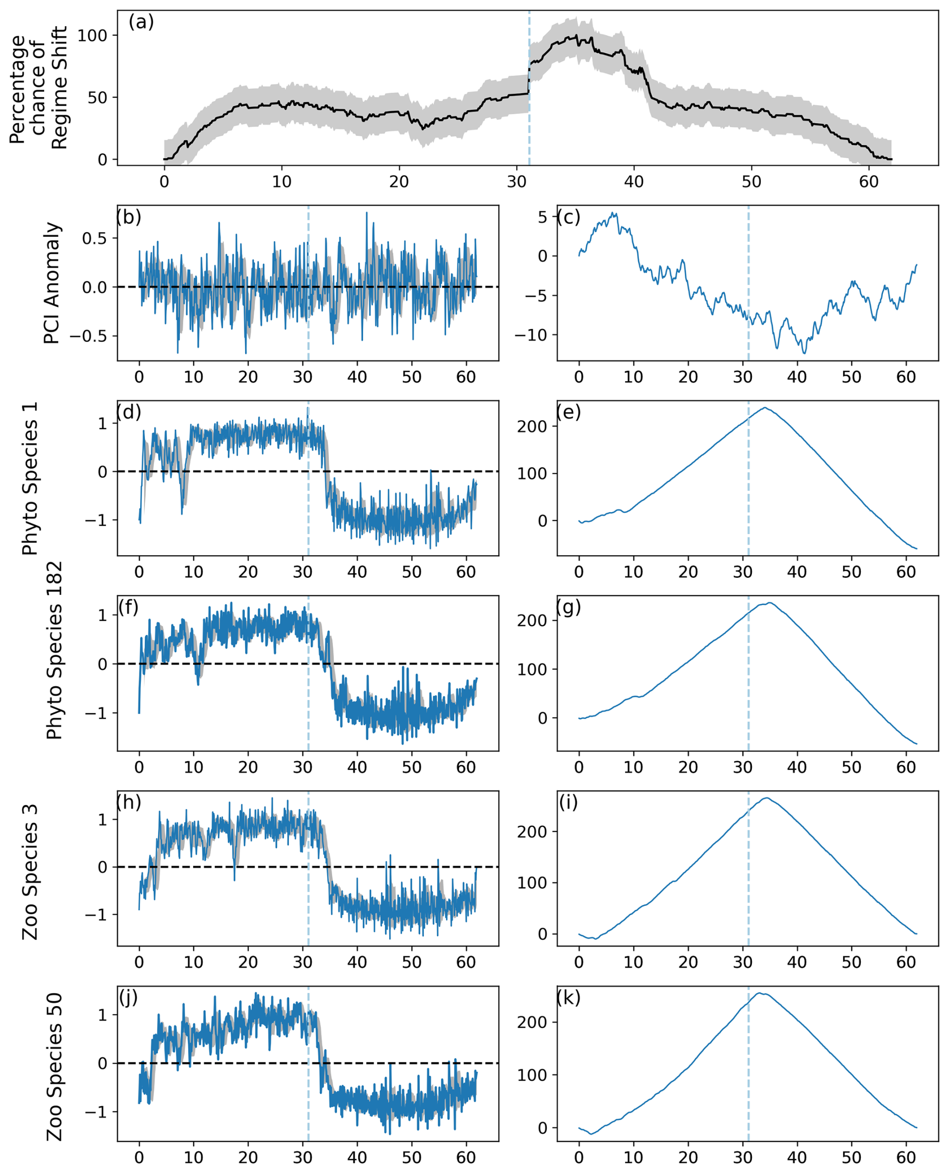
Figure 2 Output of the RST model applied to simulated data, in which a regime shift was induced in 10 % of 220 simulated phytoplankton species and 10 % of 80 simulated zooplankton species. (a) Time series of the percentage chance of a regime shift occurring, with shaded areas showing the mean absolute deviation, (b) anomalies in the simulated Phytoplankton Color Index (PCI), and (c) its cumulative sum. (d–k) Cell abundance anomalies and corresponding cumulative sums in log-transformed abundances for the (d–g) phytoplankton and (h–k) zooplankton species showing the greatest ranges in anomalies. Vertical dashed lines indicate months when the estimated regime shift likelihood changed by over 20 %. Shaded areas in (b), (d), (f), (h), and (j) represent the standard deviation around the 12-month rolling mean.

3 Validation of the model

In order to validate the RST model for its ability to detect regime shifts, a series of realistic data frames was constructed and subsequently analyzed. The RST model was designed to convert time series data into monthly mean anomalies. In validation tests this function was removed, and anomalous monthly means of species abundance were simulated using Eq. (6):

$$\begin{array}{}\text{(6)}& x\left(t\right)=\mathit{\alpha }\left(x\right(t-\mathrm{1})\cdot \mathrm{AR})+\mathit{\sigma }z,\end{array}$$

where x(t) represents the abundance of each simulated species at time step t, α is an auto-regressive coefficient used to prevent the series from moving too far from 0, kept at α=0.99, AR is the strength of autocorrelation in the time series, σ is a constant standard deviation, set to σ=0.1, and z is a random number between −1 and 1, generated at each time step.

Regime shifts were induced into a chosen proportion of the simulated data frame using Eq. 7:

$$\begin{array}{}\text{(7)}& x(t+\mathrm{1})=\left(x\right(t\left)\mathrm{AR}\right)+{\displaystyle \frac{-x(t{)}^{\mathrm{3}}+x(t)+m_t}{\mathrm{2}}}+\mathit{\sigma }z,\end{array}$$

where x(t+1) is the simulated abundance at time step t+1, m_t is a time-varying parameter that controls the regime shift dynamics, which is defined by one of three separate equations, depending on the time period, σ is a constant standard deviation, set to σ=0.2, and z is a random number between −1 and 1, generated at each time step.

The standard deviation for species in which abrupt shifts were induced was larger than for species in which shifts were not induced. The original reason for adding this effect was because it has been shown that variation increases before regime shifts caused by critical slowing down (Scheffer et al., 2001; Scheffer, 2009). It became clear that our interest should not be limited to regime shifts preceded by critical slowing down, but increasing variation for simulated species experiencing abrupt shifts resulted in increased range and a greater chance of their time series appearing in graphs (Figs. 2–7). Before any abrupt shift impacts x, m_t is equal to zero. From the beginning of the period when abrupt shifts are induced until the end of the shift, m_t gradually increases from zero until it reaches the bifurcation parameter μ:

$$\begin{array}{}\text{(8)}& \mathit{\mu }={\displaystyle \frac{\mathrm{2}\sqrt{\mathrm{3}}}{\mathrm{9}}}.\end{array}$$

The bifurcation parameter (Eq. 8) was taken from Arellano-Nava et al. (2022) in order to obtain greater control over the timing of abrupt changes. From the end of the shift until simulated abundance x returns to previous levels, m is equal to μ. In examples where x has a different behavior or abundance after an abrupt shift has taken place, m decreases gradually from the bifurcation parameter μ until −5. When m_t is equal to μ, an abrupt shift in simulated abundance is likely to occur. When m_t is decreased, abrupt shifts are unlikely.

These formulae were adapted from the original regimeshifts Python package by Arellano-Nava et al. (2022). Changes were made in Eq. (6) to allow the strength of autocorrelation to be modified, to remove the bifurcation parameter, and to allow for realistic time series that do not show a regime shift. The changes added to Eq. (7) allow for greater control of when and how long induced regime shifts take place. We performed different experiments to validate the model.

3.1 Number of species experiencing regime shifts

First, the model was tested with respect to the percentage of species experiencing a regime shift. While autocorrelation was kept at a constant level of 0.6, the proportion of simulated phytoplankton and zooplankton species in which an abrupt shift was induced was changed incrementally to show the effect of this on the percentage likelihood that a regime shift took place.

When 10 % of simulated phytoplankton and zooplankton species experienced an abrupt transition, the percentage likelihood of a regime shift remained around 50 % with little variation for the majority of the time series (Fig. 2). A regime shift was still identified just after modeled month 361, when the percentage likelihood of a regime shift occurring increased from approximately 50 % to 75 % before continuing to increase more slowly (Fig. 2).

When an abrupt shift was induced in approximately 70 % of simulated phytoplankton and zooplankton species, more dramatic increases in percentage regime shift likelihood were observed (Fig. 3). A regime shift was identified by the RST model just before the abundance of simulated PCI, phytoplankton, and zooplankton decreased (Fig. 3). The regime shift percentage likelihood increased soon after time step 361 of the simulated time series and decreased during approximately time step 460–500 (Fig. 3).

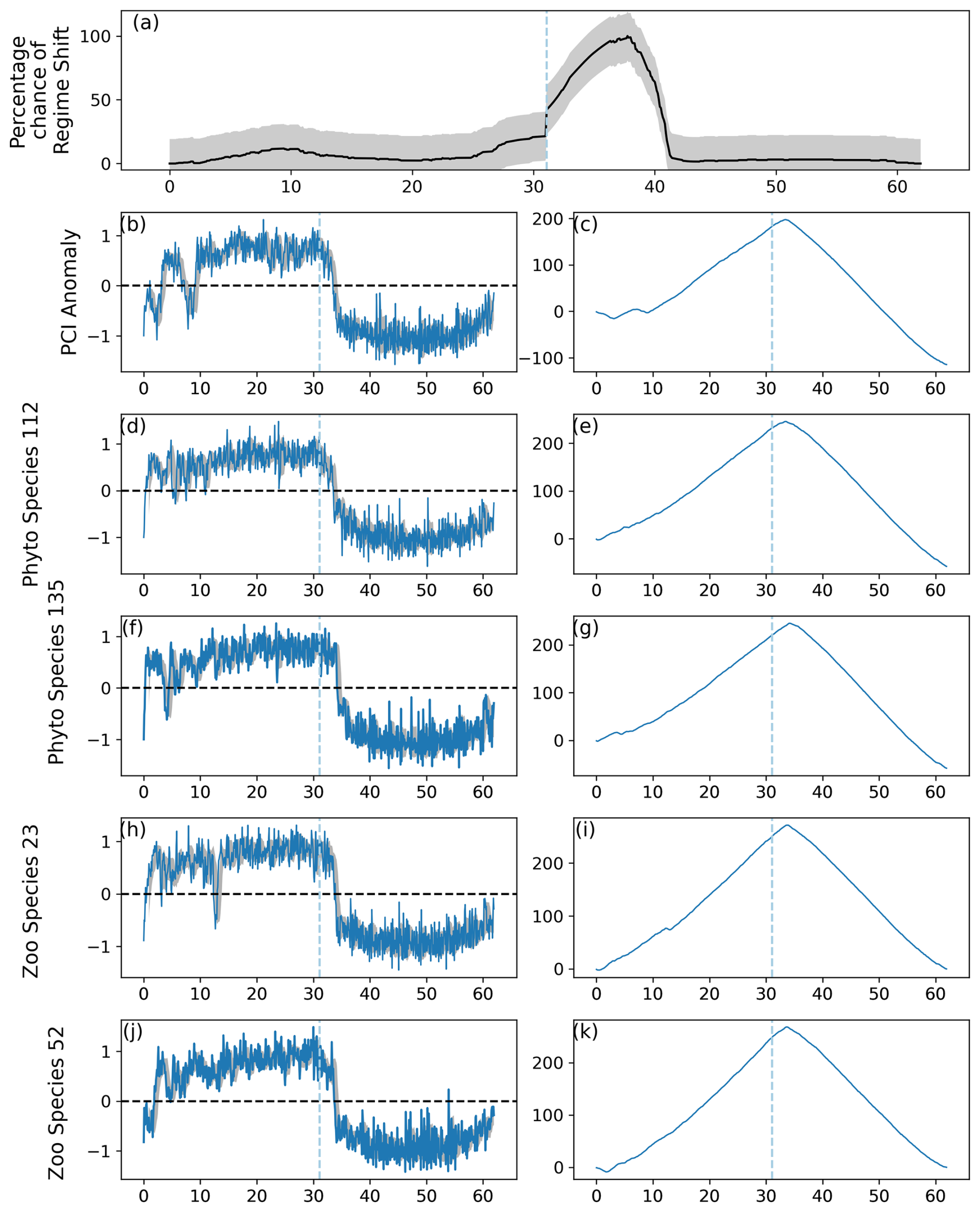
Figure 3 As for Fig. 2, except the regime shifts were induced in 70 % of simulated phytoplankton species and 90 % of simulated zooplankton species. The percentage likelihood of a predicted regime shift increased by greater than the critical gradient after simulated month 360 and continued to increase until approximately month 420. Abrupt shifts in the simulated PCI anomaly and simulated phytoplankton and zooplankton species can be observed between simulated months 0 and 150 and after 360.

3.2 Time period between induced regime shifts

Second, the effect that changing the time between induced abrupt shifts had on the percentage likelihood of a regime shift was tested. Here, the amount of autocorrelation was constantly high (0.6), and the proportion of species which experienced a regime shift was kept at a constant 0.4 while the length of time between the first and second induced abrupt changes was changed incrementally.

When the period between the first and last induced changes to simulated species abundance was restricted to lasting a maximum of 20 % of the time series, or 12.4 simulated years, the model was barely able to detect two separate regime shifts (Fig. 4). The percentage likelihood of a regime shift occurring did not decrease by more than 10 % between induced abrupt shifts (Fig. 4). When the period between the first and last induced abrupt changes was increased to being at least 22.5 % of the time series, or just less than 14 modeled years, two distinct regime shifts could be observed as the percentage likelihood fell by more than 20 % between the two induced shifts (Fig. 5).

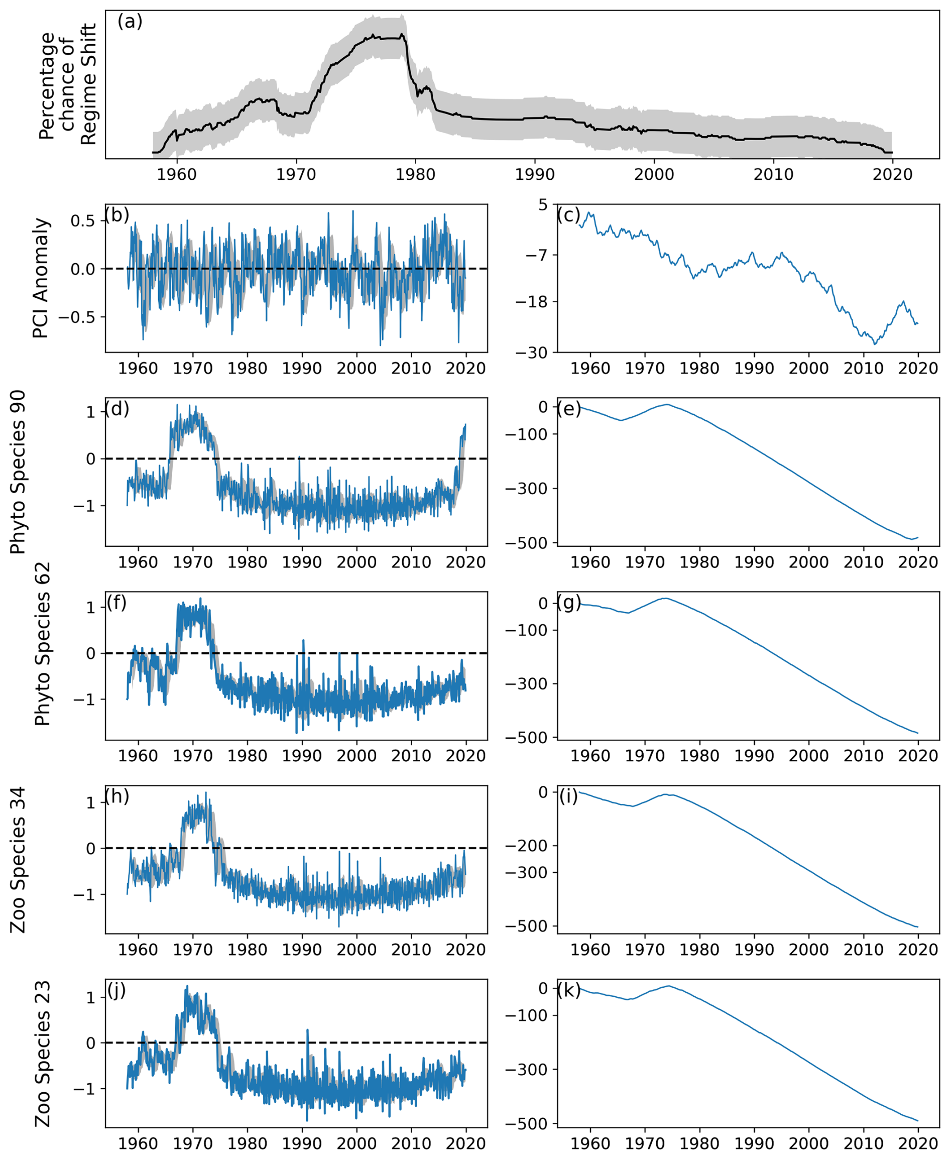
Figure 4 As for Fig. 2, except the period between first and last induced abrupt changes was restricted to last 20 % of the time series, or nearly 150 simulated months.

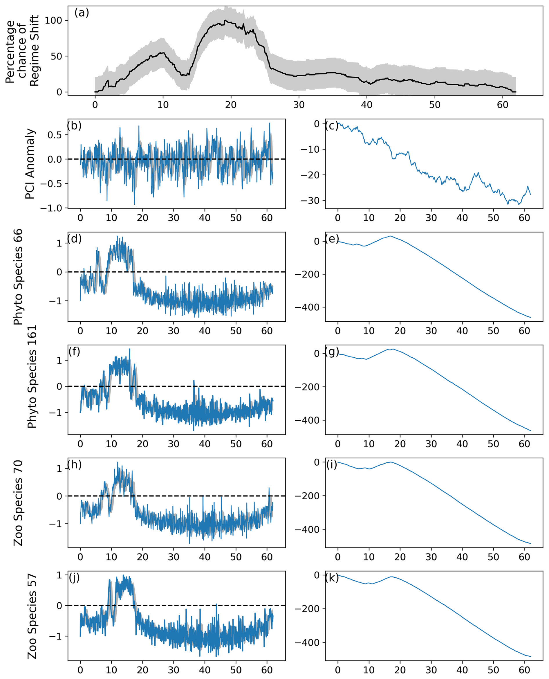
Figure 5 As for Fig. 2, except the period between first and last induced abrupt changes was restricted to 22.5 % of the time series, or 162 simulated months. The percentage likelihood of a regime shift can be observed in (a) to increase from month 150 until decreasing after approximately month 300.

3.3 Lag-1 autocorrelation strength

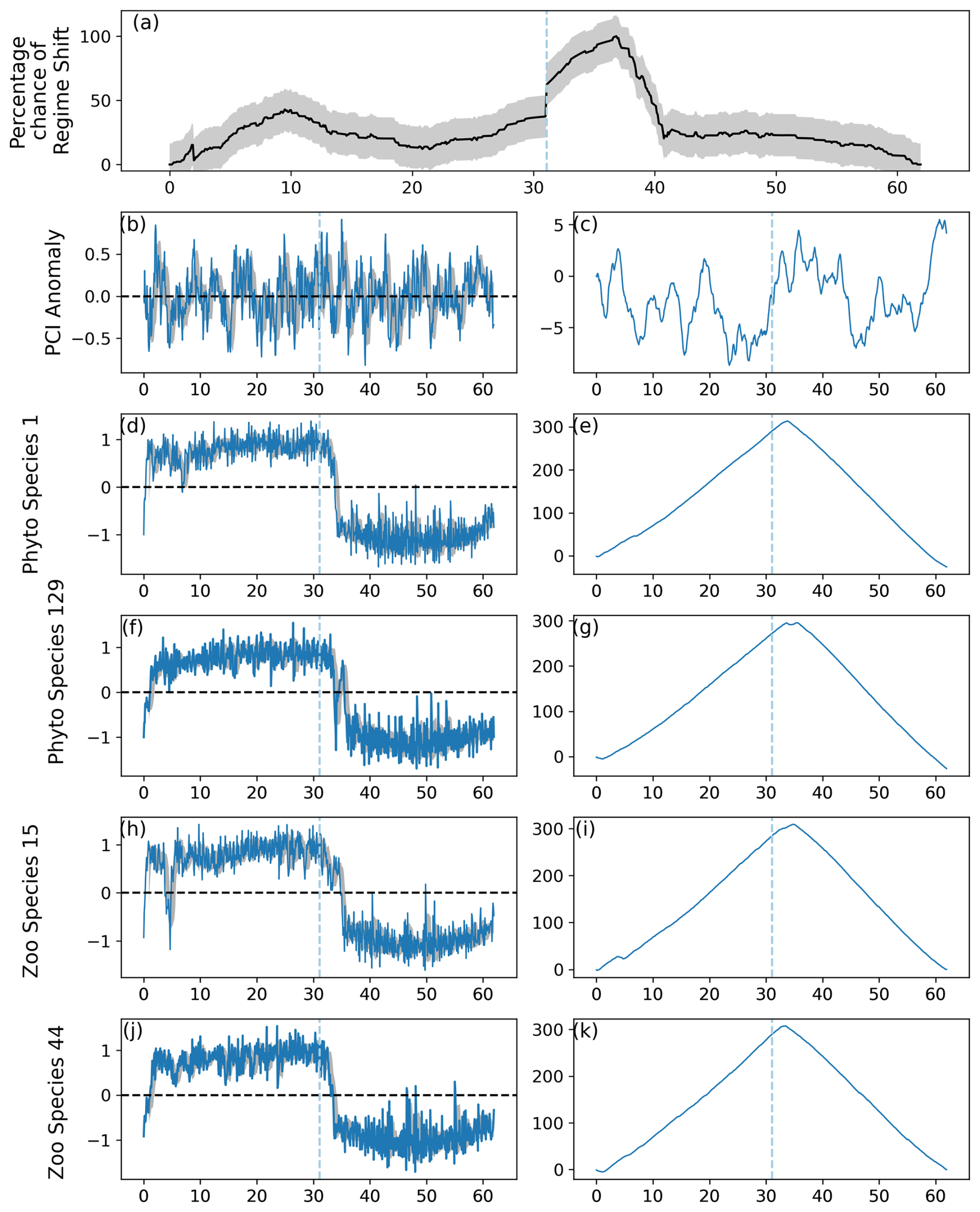
In a final validation experiment, we tested the effect of lag-1 autocorrelation strength on regime shift detectability. The proportion of species which experienced a regime shift was kept at a constant 0.4 and the time period between induced abrupt changes was also kept consistent, while autocorrelation strength was increased incrementally from 0.1 to 1.0 in steps of 0.1.

The percentage likelihood of a regime shift occurring was less variable when the strength of lag-1 autocorrelation was restricted to AR=0.1 (Fig. 6). This is especially visible at the beginning of the time series when the first abrupt change was induced, as the percentage likelihood did not increase dramatically before approximately year 25 (or month 300) of the simulation (Fig. 6). The regime shift percentage likelihood increased most dramatically after modeled month 361, when abrupt changes were induced in 40 % of phytoplankton and zooplankton species (Fig. 6).

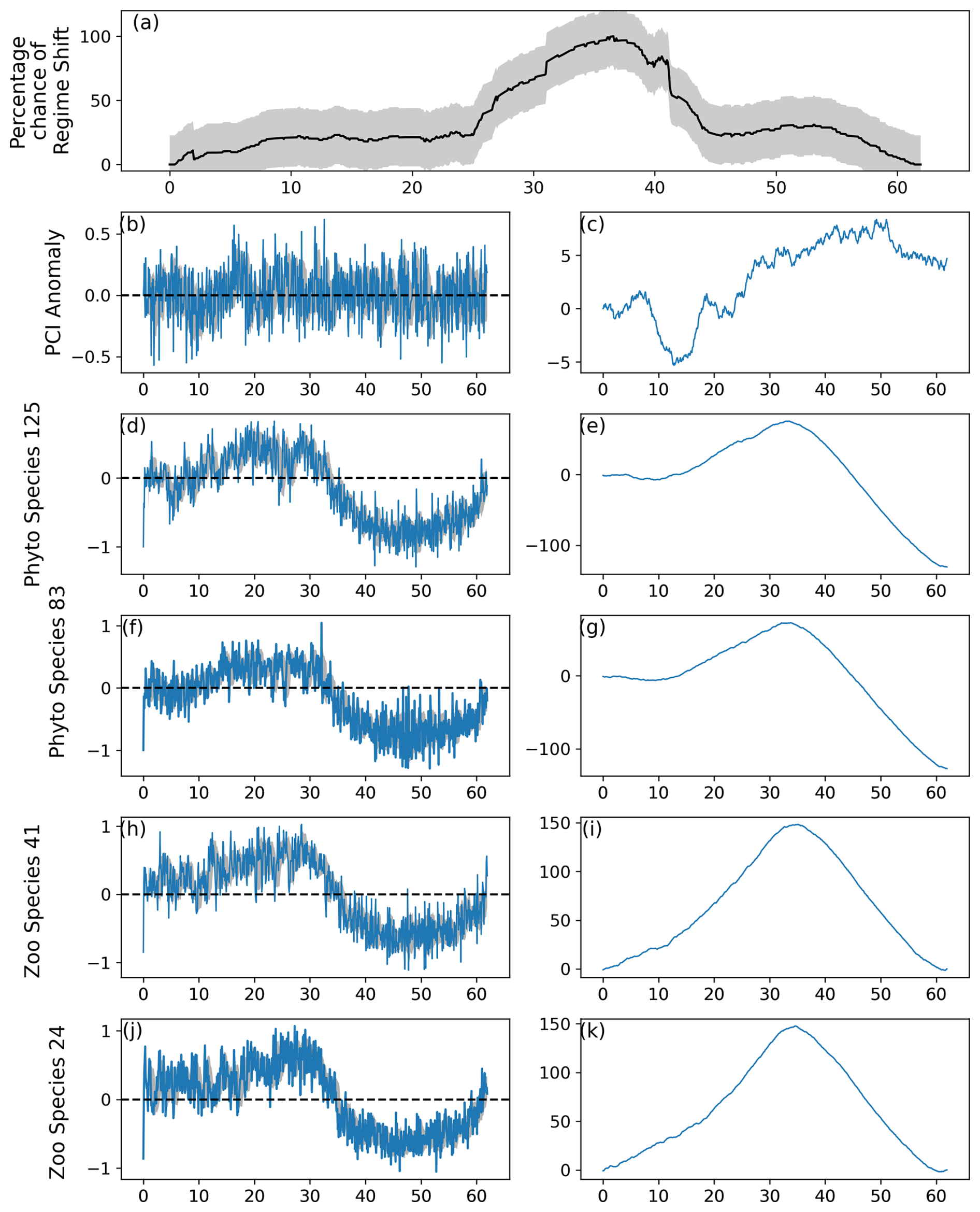
Figure 6 As for Fig. 2, except the strength of lag-1 autocorrelation was equal to 0.1. An abrupt change was not induced in the PCI anomaly (b–c), but changes were induced in species represented in (d)–(k).

When strength of lag-1 autocorrelation was increased to AR=0.725, the earlier regime shift which began after modeled month 361 was detected, as the critical gradient threshold was exceeded (Fig. 7). The maximum percentage change in a regime shift was still detected at approximately the same time as when lag-1 autocorrelation was lower, before month 481 (Figs. 6–7). A greater variation is shown throughout the time series, as the percentage likelihood was lower during periods with no induced regime shifts (Fig. 7).

Figure 7 As for Fig. 2, except the strength of lag-1 autocorrelation was equal to 0.725. A regime shift can be seen in (a) when abrupt changes can be observed in (d)–(k), just after simulated month 360.

3.4 Determination of type I and type II errors

Additional tests to determine the likely number of type I errors, or false positives, were completed using a bootstrapping model. Simulated datasets exhibiting different levels of red noise were made. This was accomplished using 100 repetitions of Eq. (6) using the same value of AR and σ but different values of the random variable z. After every 100 repetitions of Eq. (6), AR and σ were incrementally changed. AR and σ ranged between 0 and 1 and changed by steps of 0.1 and 0.2, respectively. The redness of noise was calculated using Eq. (9):

$$\begin{array}{}\text{(9)}& \mathrm{redness}={\displaystyle \frac{\mathrm{AR}}{\mathit{\sigma }}},\end{array}$$

and the redness of noise thus varied between 0.0 and 5.0.

A similar test was carried out to approximate the percentage of type II errors, or false negatives. In this example, the same bootstrapping method was used, but abrupt shifts were induced in 40 % of phytoplankton and zooplankton species using Eq. (7). To test the effect of different dataset sizes on false positive and false negative rates, experiments were repeated for datasets of 220 phytoplankton and 80 zooplankton species, 110 phytoplankton and 40 zooplankton species, and 55 phytoplankton and 20 zooplankton species. The effect of type I and type II error generation under different critical gradients was assessed by repeating these tests using critical gradients of 18 % and 20 % (Fig. 8).

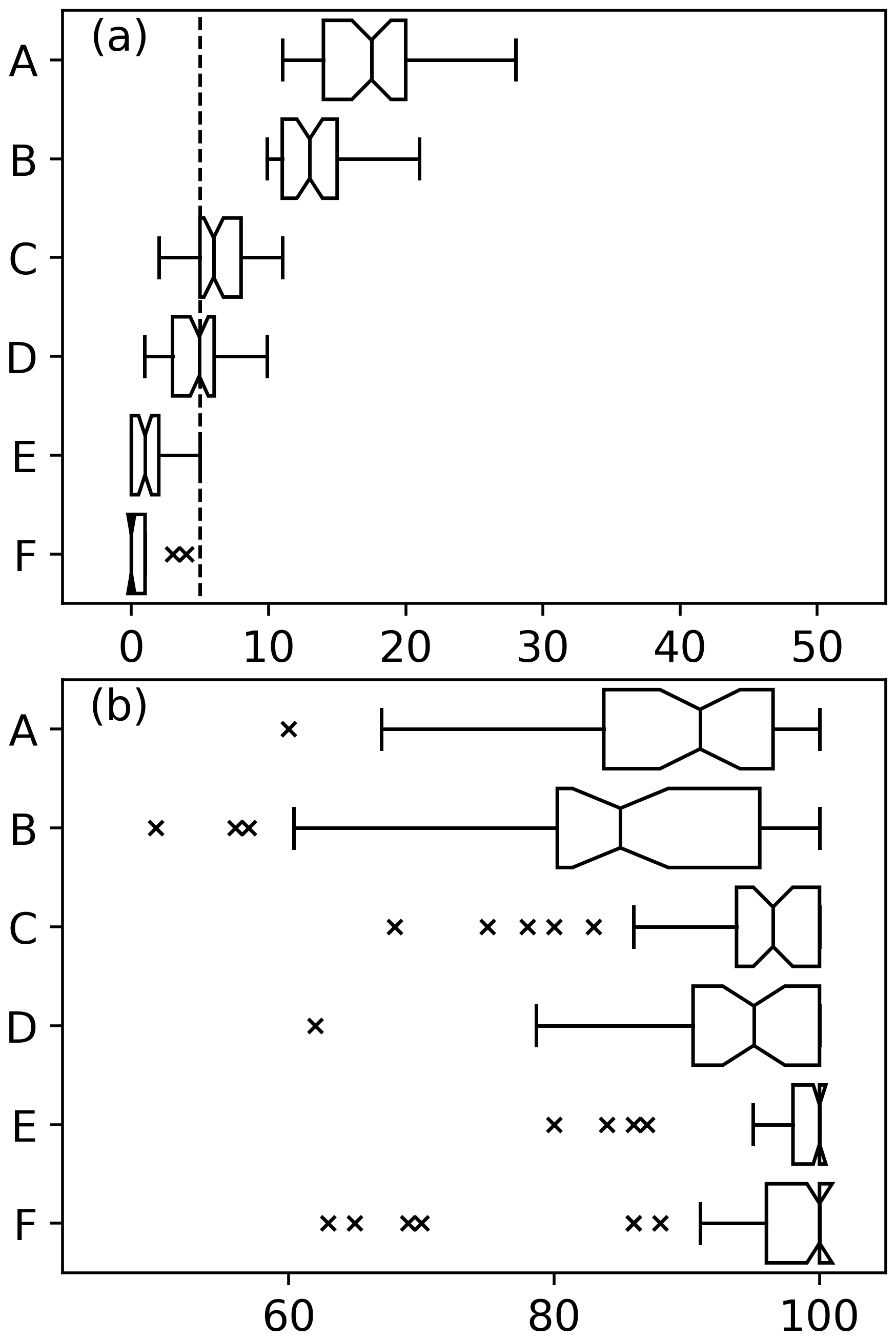
Figure 8 (a) Box plots showing the percentage of datasets of varying levels of red noise where regime shifts were identified where no abrupt changes were induced. A dashed line has been drawn at 5 %. Notches on box plots which do not overlap indicate a significant difference. Different plots show datasets of 55 phytoplankton and 20 zooplankton species where critical gradients of A 20 % and B 18 % were used to identify regime shifts, 110 phytoplankton and 40 zooplankton species where critical gradients of C 20 % and D 18 % were used to identify regime shifts, and 220 phytoplankton and 80 zooplankton species where critical gradients of E 20 % and F 18 % were used to identify regime shifts. (b) Abrupt changes were induced in 40 % of species.

Validation tests showed that the percentage likelihood of a regime shift remained high throughout nearly the whole time series when fewer species experienced abrupt shifts to their abundance (Fig. 2 compared to Fig. 3). Therefore, we chose to identify regime shifts using critical gradients instead of finding times when the percentage likelihood of a regime shift exceeded a threshold. The assumption was made that using critical gradients to identify regime shifts would result in fewer type I errors. Normalizing the results of the RST model to between 0 and 100 made the time series of regime shift likelihood in different North Sea regions more comparable but resulted in the time series being less variable and remaining high for a long time when fewer species experienced an abrupt shift (Figs. 2–3). Therefore, if the number of species in a community or ecosystem which have experienced an abrupt shift is unknown or when there is a suspicion that relatively few species have changed suddenly, it is more appropriate to use critical gradient thresholds to identify regime shifts.

We show that for datasets of 220 simulated phytoplankton species and 80 simulated zooplankton species the false positive rate is less than 5 % (Fig. 8a). The rate of false positives for datasets with fewer species is significantly higher than for larger datasets (Fig. 8). For datasets of only 55 phytoplankton and 20 zooplankton species, the choice of critical gradient results in significantly different false positive rates and false negative rates (Fig. 8). Box plots notches suggest that for smaller datasets, when a critical gradient of 20 % is used the rates of false negatives are significantly higher while false positive rates are significantly lower (Fig. 8). Differences between critical gradients of 18 % or 20 % do not appear to be significant for sample sizes of 110 phytoplankton species and 40 zooplankton species or larger (Fig. 8).

Estimates of false positive rate production demonstrates that using time series from fewer species will yield less robust results (Fig. 8). In the current example, we use time series of approximately 110 phytoplankton and 40 zooplankton species, which proved to be a sufficiently large dataset. This should be taken as an indication of the robustness of the RST model when used in the current study rather than an absolute minimum limit of the number of time series which should be used.

The original regimeshifts function by Boulton and Lenton (2019) was designed to be used by non-expert users, and we have tried to keep the same rationale. Without knowing anything about a particular community of plankton, a non-expert user could potentially input many time series into the RST model in order to identify the two most abundant phytoplankton species and whether there is a high probability of any regime shifts having taken place during the time period the dataset exists in. Apart from allowing for this process to be used by non-experts, another advantage to including all possible species is minimizing the risk of type I and type II errors by keeping sample sizes as large as possible (Fig. 8). We now show an example of using the RST model on phytoplankton and zooplankton abundance data from the CPR.

4 Case study: North Sea

After validation, the RST model was used to generate time series showing likelihood of regime shifts occurring for each of the four areas in the North Sea (Fig. 1). Abundance anomalies for each month of the time series between 1958 and 2020 were also plotted, and indications of regime shifts were plotted in each graph (Figs. 9–13). The threshold of a higher gradient change than 20 % was chosen to show when regime shifts occurred.

4.1 Identified regime shifts in area C1

A total of four regime shifts were identified in area C1, located in the center east North Sea (Fig. 1), by the RST model (Fig. 9a). These were also periods when the percentage likelihood of a regime shift occurring increased above 50 % (Fig. 9a). The four regime shifts identified were in 1989, 1997, 2002, and 2013, although of these only the identified regime shifts in 1989 and 2002 were associated with an increasing percentage chance (Fig. 9a).

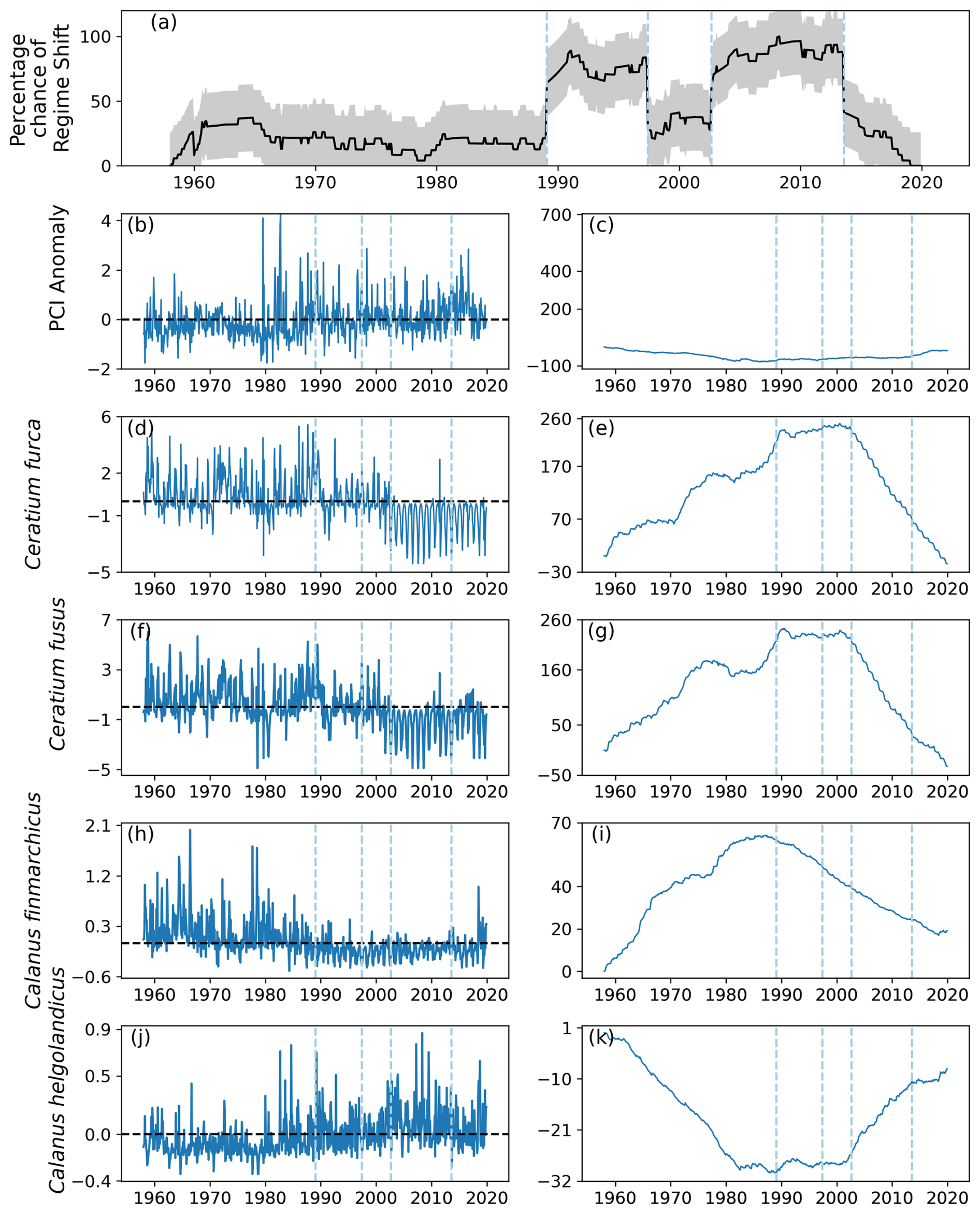
Figure 9 (a) Time series of the percentage chance of a regime shift occurring as estimated by the RST model for area C1 (see Fig. 1), located between 54 and 58° N and 3 and 12° E, (b) monthly mean anomaly, and (c) cumulative sum of PCI. (d–k) Cell abundance anomalies and corresponding cumulative sums in log-transformed abundances for the (d–g) phytoplankton species showing the greatest ranges, (h–i) Calanus finmarchicus, and (j–k) C. helgolandicus. Vertical dashed lines indicate months when the estimated regime shift likelihood changed by over 20 %. The sample size for the entire study period in this area is 11 976 (see Sect. 2).

No large variations in the PCI anomaly were detected over the study period. However, before 1990 the mean PCI anomaly was mostly just below zero (Fig. 9b–c). After 1990, the PCI anomaly was more positive (Fig. 9b–c).

Larger variations over time were detected in the abundances of the most variable phytoplankton groups, Ceratium furca and Ceratium fusus (Fig. 9d–g). Abundances of both these Ceratium species were largely above zero until 2002, when the second regime shift was identified (Fig. 9). After 2002, mean abundance of these species was below the mean abundance of the study period (Fig. 9d–g).

In contrast, the mean anomalous abundance of C. finmarchicus decreased from being mostly positive to being mostly negative in 1989, when the first regime shift was identified (Fig. 9). After 1989, the mean anomalous abundance of C. finmarchicus remained below zero (Fig. 9). At the same time, the mean anomalous abundance of C. helgolandicus increased from below zero to approximately zero in 1989 (Fig. 9). The anomalous abundance of C. helgolandicus became positive after the second regime shift began in 2003 (Fig. 9).

4.2 Identified regime shifts in area C2

Six regime shifts were detected by the RST model in area C2, located in the center west North Sea (Fig. 1): in 1963, 1980, 1989, twice in 1992, and 2003 (Fig. 10a). Of these, three were identified when the gradient of the percentage chance of a regime shifts occurring was positive: 1963, 1989, and 1992 (Fig. 10a). The percentage chance of a regime shift occurring was highest in the period between 1991 and 2003, as it remained above 75 % for most of the time (Fig. 10a).

Figure 10 As for Fig. 9, but the region of interest here is area C2 (see Fig. 1), between 54 and 58° N and between −2 and 3° E. The sample size for the entire study period in this area is 8737.

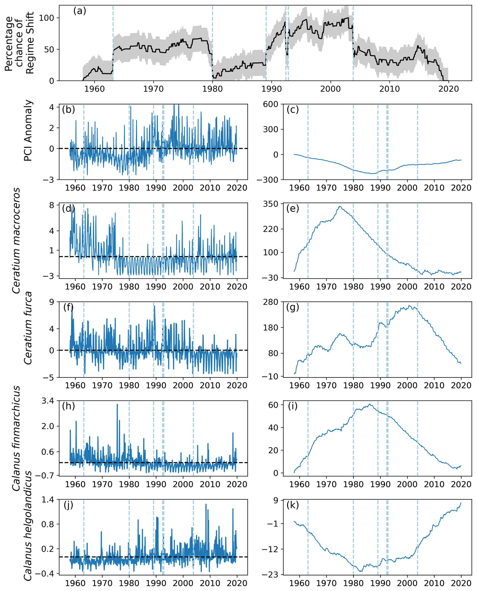
The PCI anomaly remained below zero for most of the time before 1990, after which it stayed approximately equal to zero (Fig. 10b–c). The two most variable phytoplankton species were Ceratium macroceros and C. furca (Fig. 10d–g). The mean abundance anomaly of C. macroceros was positive until the mid-1970s, after which it remained mostly negative until approximately 2003 (Fig. 10d–e). The only change in anomalous C. macroceros abundance associated with an identified regime shift occurred in 2003 (Fig. 10e). The anomalous abundance of C. furca remained around zero for most of the time series until 2003 (Fig. 10f–g). After 2003, the mean anomalous abundance of C. furca was largely below zero (Fig. 10f–g).

From the beginning of the study period until 1989, the mean anomaly of C. finmarchicus was above zero (Fig. 10h–i). After 1989, mean anomalous C. finmarchicus abundance was mostly below zero for the remainder of the time series (Fig. 10h–i). The opposite pattern was observed in the mean anomalous abundance of C. helgolandicus: from the beginning of the study period until 1980 the abundance anomaly was below zero (Fig. 10j–k). Between 1980 and 2001, the mean anomalous abundance of C. helgolandicus and the variation around it became larger (Fig. 10j–k). After 2001, the mean anomalous abundance of C. helgolandicus increased further and was almost always above zero (Fig. 10j–k).

4.3 Identified regime shifts in area D1

Two regime shifts were identified in area D1, in the southeast of the North Sea (Fig. 1). These regime shifts occurred in 1997, when there was a positive gradient, and in 2008, when there was a negative gradient (Fig. 11a). The percentage likelihood between these regime shifts remained above 50 % and was below 40 % for the remainder of the time series (Fig. 11a).

Figure 11 As for Fig. 9, but the region of interest here is area D1 (see Fig. 1), south of 54° N and between 3 and 12° E. The sample size for the entire study period in this area is 5566.

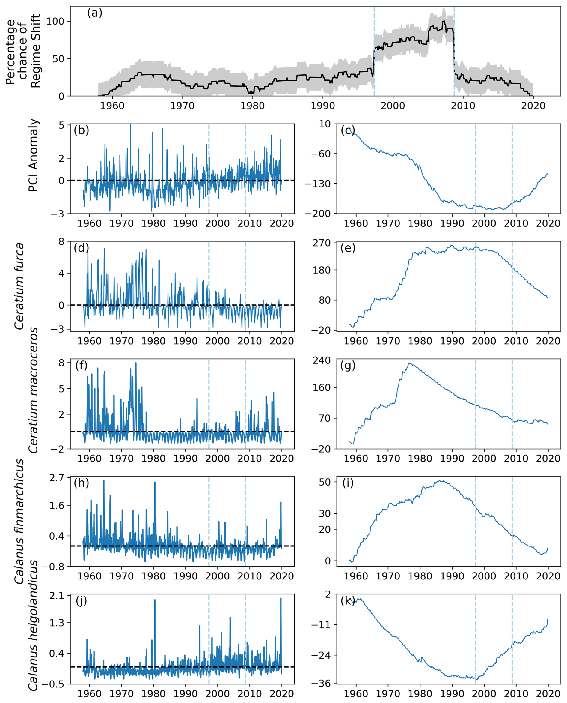
The PCI anomaly was less than zero for much of the time series until 1997 (Fig. 11b). After 2008, the mean PCI anomaly increased to above zero for the rest of the time series (Fig. 11b–c). The two most variable phytoplankton species, C. furca and C. macroceros, show positive anomalous abundance at the start of the time series until the mid-1970s (Fig. 11d–g). The mean abundance anomaly of C. furca then remained around zero until 2000, after which it decreased (Fig. 11d–e). The mean abundance of C. macroceros remained below zero from the mid-1970s until the end of the time series (Fig. 11f–g).

The anomalous abundance of C. finmarchicus was largely above zero until approximately 1988, after which it remained below zero until the end of the time series (Fig. 11h–i). The anomalous abundance of C. helgolandicus followed the opposite trend, as it stayed below zero until approximately 1988 and subsequently remained around zero until 1997 (Fig. 11j–k). After 1997, the mean anomalous abundance of C. helgolandicus increased to being mostly above zero for the remainder of the time series (Fig. 11j–k).

4.4 Identified regime shifts in area D2

Many of the patterns seen in area D1 were also seen in area D2, situated in the southwest region of the North Sea (Fig. 1). Two regime shifts were detected: during 1994, when the percentage chance gradient was positive, and 2005, when the gradient was negative (Fig. 12a). Between these identified regime shifts, the percentage likelihood of a regime shift occurring remained above 50 %, whilst it remained below 50 % for most of the rest of the time series (Fig. 12a).

Figure 12 As for Fig. 9, but the region of interest here is area D2 (see Fig. 1), south of 54° N and between −2 and 3° E. The sample size for the entire study period in this area is 9743.

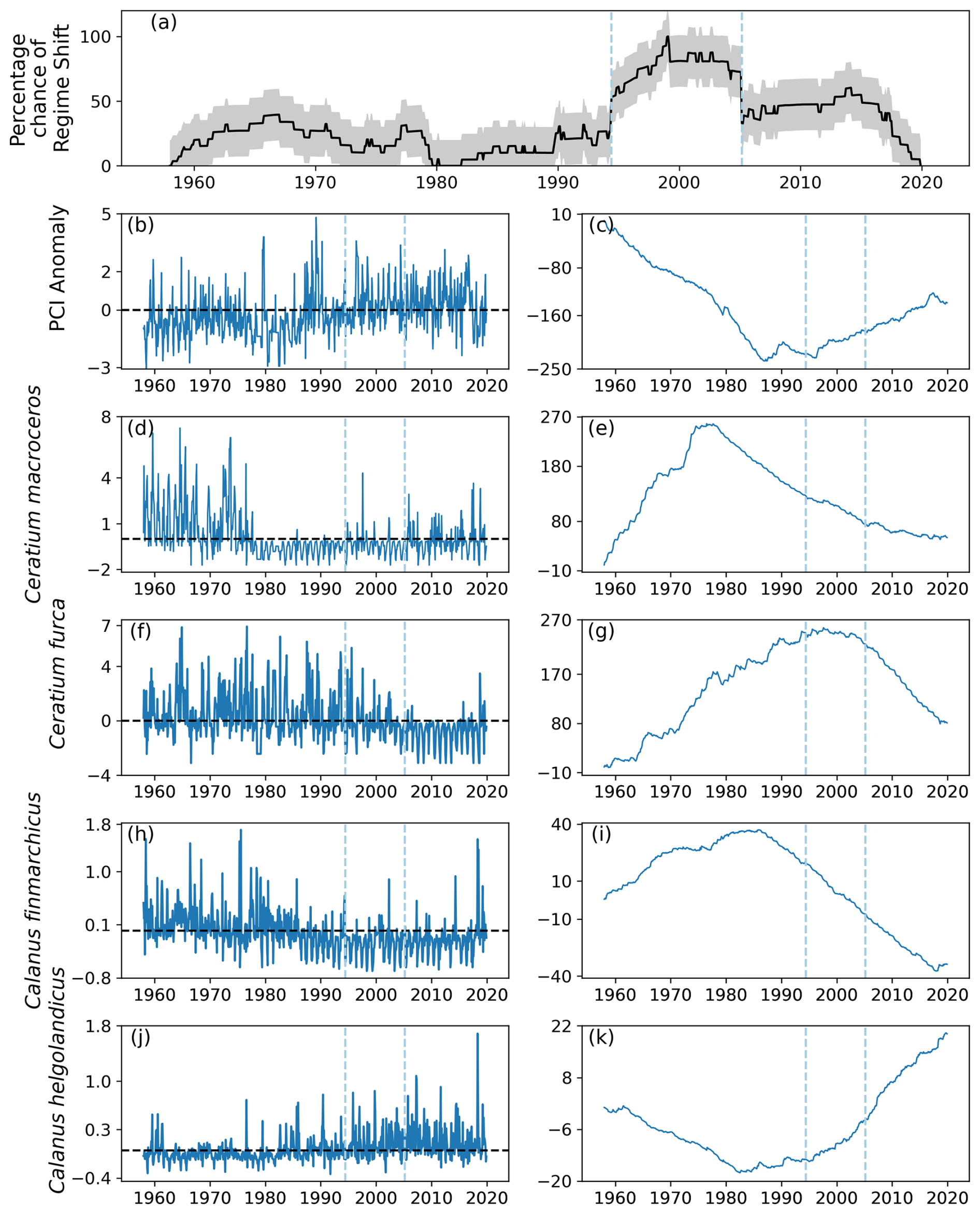
The PCI anomaly was less than zero for much of the time series until 1994 (Fig. 12b). After 1994, the mean PCI anomaly increased to above zero for the rest of the time series (Fig. 12b–c). The anomalous abundance of C. macroceros was positive at the start of the time series until the mid-1970s (Fig. 12d–e). The mean abundance of C. macroceros remained below zero until nearly the end of the time series (Fig. 12f–g). The mean abundance anomaly of C. furca remained above zero until 2005, after which it decreased to below zero (Fig. 12d–e).

The anomalous abundance of C. finmarchicus was largely above zero until the mid-1980s, after which it remained below zero until the end of the time series (Fig. 12h–i). The anomalous abundance of C. helgolandicus followed the opposite trend as it stayed below zero until approximately 1994, after which it increased to being mostly above zero for the remainder of the time series (Fig. 12j–k).

4.5 Entire North Sea

Seven regime shifts were identified for the entire North Sea (Fig. 1) by the RST model if the first is omitted for happening at the beginning. These were detected during 1962, 1972, 1979, 1998, 2003, 2008, and 2015 (Fig. 13a). Of these identified regime shifts, four of them occurred while the percentage likelihood gradient was positive: 1962, 1972, 1998, and 2003 (Fig. 13a). The percentage chance of a regime shift occurring between regime shifts was not noticeably higher or lower compared to other periods in the time series (Fig. 13a). The RST model indicated that the likelihood of a regime shift having occurred in the North Sea remained above 50 % for the majority of the time series (Fig. 13).

Figure 13 As for Fig. 9 but showing results of the entire North Sea (Fig. 1). The sample size for the entire study period in this area is 56745.

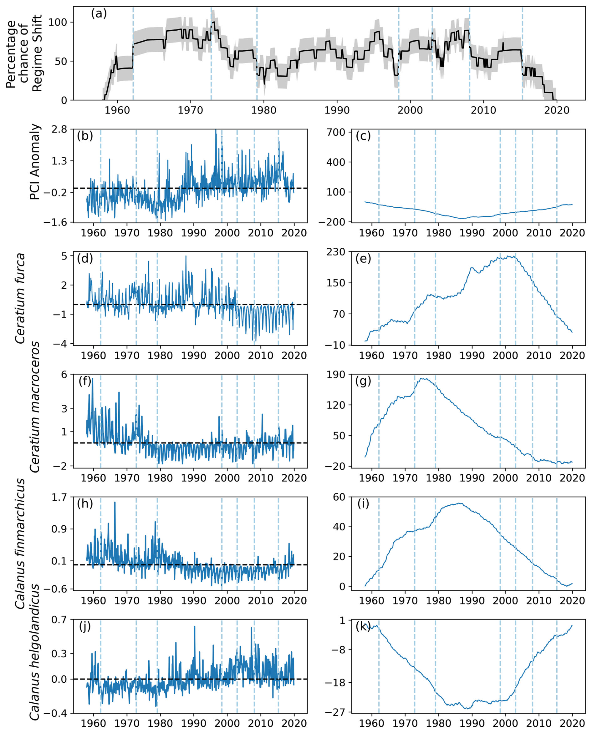
The mean PCI anomaly in the North Sea began to increase above zero in approximately 1980 (Fig. 13). From approximately 1990 until the end of the study period, the PCI anomaly remained relatively steady.

The two most variable phytoplankton species, C. furca and C. macroceros, exhibited more dramatic changes in abundance. These changes occurred just after 2000 for C. furca, and between 1970 and 1980 for C. macroceros (Fig. 13d–g). Each of these abrupt shifts were associated with regime shifts identified by the RST model (Fig. 13d–g).

The abundance of C. finmarchicus began to decrease between 1980 and 1990, at approximately the same time that the PCI anomaly started to increase (Fig. 13). The decrease in C. finmarchicus was preceded by the abundance of C. helgolandicus starting to increase (Fig. 13). It is difficult to attribute any of these changes to regime shifts identified by RST, but when C. helgolandicus started to increase from just before 2000, the probability of a regime shift occurring increased by more than 20 % per month several times (Fig. 13).

4.6 Summary of North Sea results

The RST model successfully identified regime shifts in the North Sea, and their variance over time, space, and species involved (Tables 1–2). Regime shifts identified by the RST model in the beginning of the study period appear to have been accompanied by changes in phytoplankton species abundance, though not necessarily the PCI anomaly (Table 1). Regime shifts in the 1980s and 1990s appear to have been accompanied by changes in copepods C. finmarchicus and C. helgolandicus and in the PCI anomaly (Table 1). Regime shifts after 2000 appear to be associated with changes in phytoplankton species abundance (Table 1).

Table 1 Regime shifts identified by RST model, divided into 20-year periods. The species involved column indicates whether the PCI anomaly, the two most variable phytoplankton species, or either C. finmarchicus or C. helgolandicus experienced noticeable changes associated with the identified regime shift.

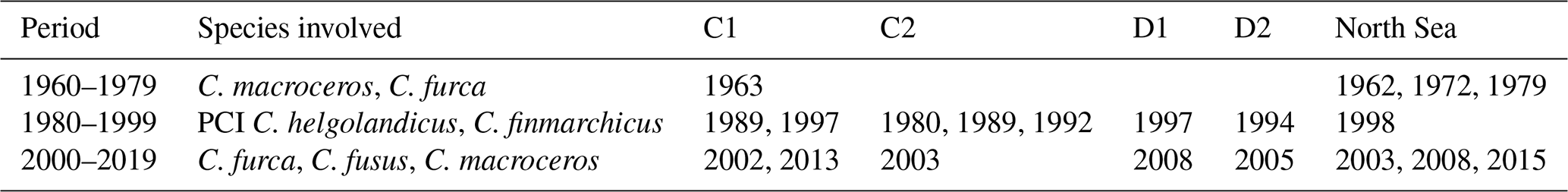
Table 2 Comparison of regime shifts found in North Sea areas during the present study.

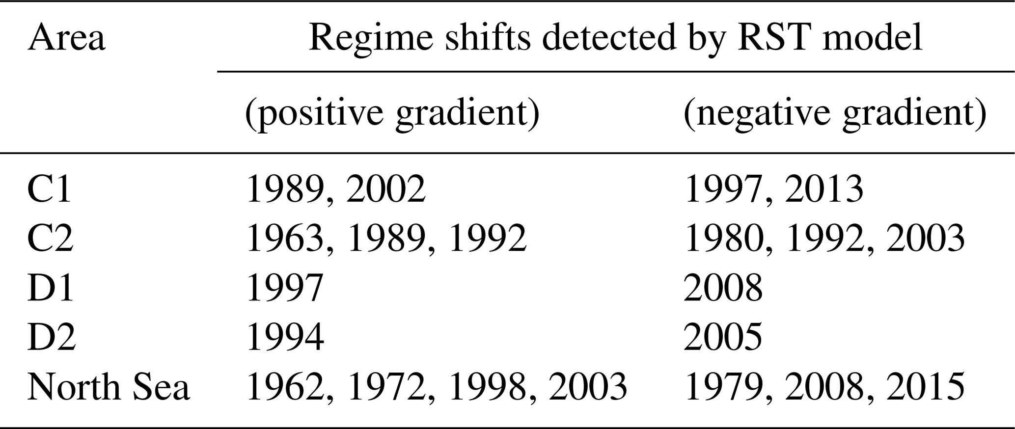
In the south of the North Sea, identified regime shifts were first observed in the west in area D2 before the east in area D1 (Tables 1–2). In the center of the North Sea, it is more difficult to determine whether the same regime shifts were detected at similar times, as more were detected by the RST model than in the south (Table 2).

Abrupt changes in the PCI anomaly, the abundance anomaly of either of the two most variable phytoplankton species, or at least one of C. finmarchicus or C. helgolandicus were detected when the majority of regime shifts were identified if the gradient of regime shift likelihood was positive (Table 2). Exceptions occurred in D2 during 1994 and in the North Sea during 1962 and 1972 (Figs. 12–13; Table 2). Similarly, regime shifts were identified when the likelihood time series gradient was negative, which were not accompanied by abrupt changes in the PCI anomaly or the other four time series shown. An example of this was in area C2 during 1989 (Fig. 10). Exceptions appear to occur regardless of whether the RST gradient is positive or negative; so, all times when the critical gradient was exceeded have been noted (Tables 1–2).

5 Discussion

Our analysis presents a novel multispecies approach to quantify the likelihood of a regime shift occurring in marine plankton communities. We find that by constructing a single time series of regime shift likelihood from abundance data of different phytoplankton and zooplankton species, our model is able to reliably detect previous regime shifts in the North Sea (Table 1). Distinguishing regime shifts in North Sea plankton from changes in abundance due to advection is a limitation of this approach. Future work could address this limitation by incorporating spatial patterns from hydrodynamic models, helping to separate genuine ecological shifts from transport-driven variability. A step towards this would be to divide the North Sea into hydrodynamically appropriate regions (van Leeuwen et al., 2015), but this is beyond the scope of the present study. A single time series of regime shift likelihood may lead to the future development of automated detection algorithms. Comparison of regime shift likelihood to potential drivers in a single-variate model is likely to be less challenging to implement than multivariate models or principal component analyses.

5.1 Proof of concept

As noted by multiple ecological studies, validation of new methods and models is a necessary first step (Dees et al., 2023; Mateus et al., 2019; Groesser and Schwaninger, 2012). We therefore constructed artificial abundance data that mimic the characteristics of observed CPR data, which allowed for extensive validation of our model, an approach successfully applied in the multi-scale multivariate split moving window methodology to identify North Sea regime shifts (Beaugrand et al., 2014). Further, we estimated the probability of our model producing type I and II errors in order to quantify the robustness of our model's ability to detect regime shifts, which Haines et al. (2024) have identified as a frequent limitation of regime shift detection models.

Validation tests showed that regime shift likelihood variation during induced regime shifts was much larger when a greater proportion of species experienced an abrupt change. When only a small proportion of species experience an abrupt abundance shift, the percentage of regime shift likelihood remained high for a large part of the time range and only deviated by just over 20 %. This is important to know for interpretation of RST output when ecological data are used. Previous studies have shown that for plankton populations in the North Sea, approximately 40 % of species were involved in identified regime shifts (Beaugrand et al., 2014). We have shown that the model can detect regime shifts when fewer species are involved, but care must be taken when interpreting model output as the 20 % critical gradient is not always exceeded.

The minimum amount of time between abrupt shifts that the RST model was able to distinguish was between 12 and 14 years. The time period between abrupt changes was therefore kept at 40 % of the time series, or just under 25 years, to remove all possibility of the time taken for the community to be established having an impact on model performance. It is likely that for abrupt changes with a time period between them of less than 12 years, the predicted likelihood of a regime shift will be elevated over an extended time period. Another observed limitation of the model is the length of time between the start of the time series and when the earliest regime shift can be detected. In Fig. 7, abrupt changes to the abundance of two phytoplankton species can be observed but were not accompanied by an increase in the regime shift probability time series above the critical gradient. This is similar to Beaugrand et al. (2014), where results suggested a regime shift near the beginning of their study period which could not be confirmed.

Autocorrelation in time series data can lead to increased false positive rates (Haines et al., 2024). Removal of the effect of autocorrelation has previously been accomplished using statistical means such as the modified Chelton method, which reduces the number of degrees of freedom (Pyper and Peterman, 1998; Hinder et al., 2014; Bedford et al., 2020a; Dees et al., 2017), or by applying an auto-regressive-moving average (ARMA) model to the data (Alvarez-Fernandez et al., 2012). The original regimeshifts model, incorporated within the RST model described here, does not remove autocorrelation but instead detects anomalous rates of change (Boulton and Lenton, 2019; Arellano-Nava et al., 2022). Similar to tipping points, regime shifts can be preceded by increasing autocorrelation and variance (Dakos et al., 2015; Scheffer et al., 2001). Preserving autocorrelation within the analyzed dataset is therefore preferential when looking for early warning signals for regime shifts. Regime shift detection by the RST model is improved when autocorrelation is stronger, although in silico validation tests have shown that regime shifts are still identified when the autocorrelation before abrupt shifts is weak or absent. Preserving more of the dataset's original structure appears to allow for the RST model to identify regime shifts with a low false positive rate relative to other methods (Fig. 8) (Haines et al., 2024; Rudnick and Davis, 2003).

The in silico experiments described here show that the RST model is capable of identifying regime shifts with similar numbers of species as is collected by the CPR, but care should be taken if the time series of regime shift likelihood does not deviate dramatically. Changes in regime shift likelihood of approximately 20 % should be investigated individually by looking at accompanying time series and cumulative sum graphs, as it is possible that these are false positives or false negatives.

The RST model identified likely regime shifts in different regions of the North Sea, which can be grouped by species and timing. Regime shifts observed at the beginning and end of the study period appear to have been caused primarily by changes in the most abundant species of phytoplankton. Regime shifts in the 1980s and 1990s appear to have been driven by changes in the PCI and copepods C. finmarchicus and C. helgolandicus. These results are consistent with previously identified regime shifts in the North Sea (Beaugrand et al., 2014; Djeghri et al., 2023; Bedford et al., 2020a; McQuatters-Gollop et al., 2007), although it is difficult to make a direct comparison due to differences in spatial areas chosen.

The North Sea and the distribution of any plankton within it are influenced by advection (Hjøllo et al., 2009; Fransz et al., 1991; Bartsch et al., 1989), and it is premature to conclusively identify a particular date when a regime shift occurred without comparing neighboring areas. For example, results from the RST model show an apparent regime shift involving C. finmarchicus and PCI occurred in the mid-west of the North Sea (area C2) during 1992, subsequently in the southwest of the North Sea (area D2) during 1994, and then in the southeast North Sea (area D1) during 1997. Again, a regime shift involving C. macroceros, C. furca, and C. fusus was identified in area C2 in 2003, then in D2 during 2005, before being detected in D1 in 2008. An important limitation of the RST model is that it is difficult to confirm whether regime shifts have taken place at different times or rather abrupt changes in plankton were due to advection around the North Sea system.

One of the first investigations of ecological regime shifts in the North Sea focused on the shift from a zooplankton community dominated by C. finmarchicus to one where C. helgolandicus was more dominant in the North Sea between 1982 and 1989 (Beaugrand and Reid, 2003; Reid et al., 2016, 2001). Other studies have suggested this regime shift began later in the 1980s (Wouters et al., 2015; Beaugrand, 2014; Alvarez-Fernandez et al., 2012). More investigations into North Sea plankton communities revealed another likely regime shift which ended in 1968, though as this was the near the beginning of the ecological time series used there is less confidence (Beaugrand, 2014). A final ecological regime shift was identified between 1996 and 2003, though whether there was an impact on ecosystem function is uncertain (Beaugrand et al., 2014; Djeghri et al., 2023; Alvarez-Fernandez et al., 2012). When analysis into separate northern and southern North Sea areas took place, a regime shift was detected around 1978 (Alvarez-Fernandez et al., 2012). Using the RST method we have shown three periods of increased regime shift likelihood, though likelihood differs by North Sea area.

For the entire North Sea, the RST model detected regime shifts at similar times to Beaugrand et al. (2014). However, the split moving window method did not detect regime shifts after 2003 (Beaugrand et al., 2014). When just area C1 of the North Sea was considered, the RST model detected the regime shifts in the late 1980s, and between the late 1990s and early 2000s. Again, a later regime shift after 2010 was also identified. The RST model also detected the late 1980s shift in area C2. Interestingly, Alvarez-Fernandez et al. (2012) detected regime shifts in approximately 1978 which appear consistent with those detected by the RST model in the entire North Sea in 1979 and area C2 during 1980. The shift from C. finmarchicus to C. helgolandicus appears to have occurred later in areas D1 and D2. Further study of the plankton community and the apparent regime shifts suggested in many areas after 2003 is recommended.

5.2 RST model output

The nature of the CPR database and the RST model's ability to detect regime shifts in multispecies communities means that abrupt changes in phytoplankton and zooplankton species that were not displayed in the output's graphs can be identified. Equation (7) induces regime shifts in simulated time series, but the stochastic term m incorporated within Eq. (7) gradually increases the likelihood of a simulated time series to experience an abrupt change. For example, minor differences in the timing of abrupt shifts in phytoplankton species 1 and 129 and zooplankton species 15 and 44 can be observed. In this case, abrupt changes began to be induced in 40 % of species just before 1990, which caused the percentage likelihood of a regime shift to increase. The RST time series shows the probability of the entire plankton community captured by the CPR experiencing a regime shift and is influenced by abrupt shifts in individual species. The ability to calculate the risk of regime shifts in the community by analyzing all species, instead of those assumed to be most important, exhibits the importance of the RST model.

Large and dramatic changes in species abundance can occur without an accompanying change in regime shift likelihood, as observed in C. finmarchicus abundance in the entire North Sea, and either Ceratium spp. or PCI in area D1. The RST model is designed to predict regime shift likelihood for all species that are input, and changes to single species do not always affect the entire community (Fauchald et al., 2011; Djeghri et al., 2023). This is an important difference from other regime shift detection algorithms used in the North Sea (Beaugrand et al., 2014; Bedford et al., 2020a, b). Output from the original regimeshifts function was multiplied by the mean abundance of species for that month, resulting in the RST model estimating regime shift likelihood for all species in a particular database rather than simply measuring the number of species exhibiting abrupt changes. In this way, the RST model was kept appropriate for non-expert users while scaling the proportion that each species contributes to the percentage likelihood of a regime shift. Applying more specific weights to keystone species such as C. finmarchicus or C. helgolandicus may be an interesting avenue for future research.

In contrast to the present study, which used abundance records from every species recorded in the CPR dataset, previous studies identifying regime shifts in marine plankton datasets have looked at small groups of individual species. Example studies include those analyzing the 1980s regime shift involving C. finmarchicus and C. helgolandicus (Beaugrand and Reid, 2003; Edwards et al., 2001; Reid et al., 2016) and those studies grouping species into functional groups of phyto- and zooplankton (Beaugrand et al., 2014; Bedford et al., 2020a; Hinder et al., 2012; McQuatters-Gollop et al., 2007; Haines et al., 2024). The advantage of this approach is the ability to show how certain groups of species have changed over time, possibly as a response to increased temperature or increases in other anthropogenic input (Bedford et al., 2020a; Beaugrand and Reid, 2003; Edwards et al., 2001). However, by looking at only a limited number of species or groups, studies can miss changes to other species groups which were not specifically checked. It is particularly difficult to calculate major changes across multiple trophic levels in the marine environment because different sampling methodologies are used for plankton and fish and data have often been collected over different scales of time and space (Haines et al., 2024; Beaugrand and Reid, 2003; Reid et al., 2001). Studies of ecological regime shifts have therefore traditionally been more common in closed systems like lakes, where regular monitoring of across multiple regime shifts is easier (Bertani et al., 2016). Ecological regime shifts in marine ecosystems should be observed at more than one trophic level at a time (Beaulieu et al., 2016; Yletyinen et al., 2016; Haines et al., 2024).

Assessing how many trophic levels are represented in a database of phytoplankton and zooplankton is challenging, as heterotrophic dinoflagellates can be an ecologically significant consumer of ciliates, diatoms, and some smaller zooplankton species (Sherr and Sherr, 2007; Park et al., 2006). Accordingly, zooplankton can operate over a range of trophic levels depending on species, season, and region (Kürten et al., 2013; Décima, 2022). The methodology of Ibanez and Dauvin (1998) to select species from the CPR dataset focused on choosing representative species and avoiding zero inflated presence–absence counts. Use of this selection methodology meant that only 44 phytoplankton species and 29 zooplankton species were analyzed using the method of Beaugrand et al. (2014). In contrast, the present method used data from all species collected by the CPR. At least three trophic levels were thus included: phytoplankton, zooplankton, and fish larvae and eggs.

In order to take greater advantage of the valuable CPR dataset and all trophic levels included, the RST model used in this analysis explicitly placed exponentially greater weight on the percentage likelihood of a regime shift if abrupt changes were detected in both phyto- and zooplankton species within the window length of 24 months (see Methods). When data for the entire study area were analyzed by the RST, the percentage likelihood of a regime shift taking place was highest in approximately 1968, the late 1980s, and between 1996 and 2003. These periods compare favorably with those identified by Beaugrand et al. (2014) and provide some validation of the RST model described here. Explicitly adding differing weights to meroplanktonic organisms may be an interesting avenue of future research.

5.3 Robustness of regime shift detection

A recent paper looking at various different methodologies for detecting regime shifts in marine ecosystems showed that most methods generate false positives at such a high rate that it is impossible to determine whether regime shifts in the North Sea and along the west coast of Norway have really taken place (Haines et al., 2024). Some regime shift detection methods produce false positive rates of 100 %, though the majority are closer to around 20 % (Haines et al., 2024). Although the present model does not always have a false positive rate below 5 %, the false positive rate when using the RST model is lower than those reported by a range of previous studies (Haines et al., 2024; Rudnick and Davis, 2003). Results presented in the present study suggest when more species are analyzed, there is a reduced likelihood of generating false positives or negatives. The lower false positive rate shows the value of including all species collected by the CPR.

It has been assumed that the production of type II errors detracts from model usefulness more than type I error production does, particularly as false positives have been reported more commonly (Haines et al., 2024; Rudnick and Davis, 2003). The rate of false negatives in the present study is higher than those for false positives. Decreasing the value of the critical gradient used to identify regime shifts in this study will likely decrease false positive production, but validation tests performed in this study indicate doing so will increase the rate of false negatives. Having a conservative estimate of regime shift likelihood should increase the certainty in identified regime shifts. If this method is used to predict regime shifts in future scenarios or management situations, further reducing false positives could lead policy makers to perhaps wrongly assume a regime shift is not imminent when one could occur in the near future. We therefore advise RST model users to thoughtfully explore the use of different window lengths and critical gradients, especially if using the model to advise management.

Thoughtfully interpreting graphs generated by the RST model alongside species abundance data, instead of only noting times when the critical gradient indicates that a regime shift is likely, will also help identify false positives and negatives. The resultant time series generated by the RST of a dataset with no induced abrupt changes shows much less variation and fewer large changes over a study period compared to a dataset with more species experiencing abrupt changes. Using examples like this as a comparison can help users of the RST model to identify spurious regime shifts identified using gradients or thresholds.

6 Conclusion

The RST model described here has shown success at identifying regime shift probability in a single time series based on patterns of species abundance, and whether abrupt changes in abundance are observed in more than one trophic level. Validation tests have demonstrated the robustness of the RST model and its ability to identify regime shifts with a relatively low error rate. Recent advances in machine learning and deep learning algorithms mean that forecasting single time series into the future is a possibility which should be explored in future studies (Hewamalage et al., 2023). Success in this endeavor will show the RST model described here as a first step to designing a regime shift forecasting model for the 21st century.

Although there are several advantages to condensing an estimate of regime shift likelihood into a single time series, limitations of this approach have also been discussed. These limitations include needing approximately 14 years between abrupt changes for the algorithm to detect regime shifts and the inability to distinguish between apparent regime shifts caused by advection. Another potential disadvantage of reducing the rich data collected by the CPR into one time series is removal of context, which can potentially introduce more uncertainty and biases into the estimation of whether a regime shift occurred (Nguyen, 2024). For example, a recent study on the northwest European shelf found no change in functional groups associated with past identified regime shifts (Djeghri et al., 2023). Another study has found evidence that functional groups have changed but did not link this to abrupt regime shifts (Bedford et al., 2020a). Links between regime shifts in plankton and fish do exist (Reid et al., 2001; Vollset et al., 2022) and there is even evidence to suggest regime shifts have affected the abundance of organisms from higher trophic levels, such as whales (Meyer-Gutbrod et al., 2021). Further studies of regime shifts in plankton communities should elucidate whether such regime shifts are drivers of regime shifts in higher trophic levels or rather that abrupt changes seen in more than one trophic level are caused by the same biotic or abiotic drivers.

The relatively low variability observed in regime shift likelihood for the entire North Sea when compared to the smaller subregions, which have much smaller sample sizes, is likely to be due to regime shifts occurring in different parts of the North Sea at different times. The North Sea is a semi-enclosed body of water where the distribution of plankton is influenced by water advection (Hjøllo et al., 2009; Bartsch et al., 1989; Fransz et al., 1991). There is also a diverse range of hydrodynamic regimes in the North Sea, distinguished by stratification patterns and freshwater influence (van Leeuwen et al., 2015). The standard regions used in most studies of CPR data (Djeghri et al., 2023; Beaugrand, 2014; Beaugrand et al., 2010; Bedford et al., 2020a), including the present study, are likely not as ecologically meaningful in comparison to regions divided based on similar ecohydrology or distance from inflow channels. A 21st century early warning system for regime shifts should make use of subareas divided by hydrology and distance from north or south entrances to the North Sea. This would improve our understanding of physical drivers of regime shifts and contribute to more advanced regime shift prediction.