Process-based modelling of nonharmonic internal tides using adjoint, statistical, and stochastic approaches – Part 2: Adjoint frequency response analysis, stochastic models, and synthesis

Internal tides are known to contain a substantial component that cannot be explained by (deterministic) harmonic analysis, and the remaining nonharmonic component is considered to be caused by random oceanic variability. For nonharmonic internal tides originating from distributed sources, the superposition of many waves with different degrees of randomness unfortunately makes process investigation difficult. This paper develops a new framework for process-based modelling of nonharmonic internal tides by combining adjoint, statistical, and stochastic approaches and uses its implementation to investigate important processes and parameters controlling nonharmonic internal-tide variance. A combination of adjoint sensitivity modelling and the frequency response analysis from Fourier theory is used to calculate distributed deterministic sources of internal tides observed at a fixed location, which enables assignment of different degrees of randomness to waves from different sources. The wave phases are randomized by the statistical model from Part 1 using horizontally varying phase statistics calculated by stochastic models. Essential inputs of the model suite are barotropic tidal currents, background stratification, and the variance and spatial correlation of internal-tide phase speed. An example application to nonharmonic vertical-mode-one semidiurnal internal tides on the Australian North West Shelf shows that (i) phase-speed variability primarily makes internal tides nonharmonic through phase modulation, and (ii) important controlling parameters include the variance and correlation length of phase speed, as well as anisotropy of the horizontal correlation of phase modulation. The model suite also provides a map of nonharmonic internal-tide sources, which is convenient for identifying important remote sources, such as the Lombok Strait in Indonesia. The proposed modelling framework and model suite provide a new tool for process-based studies of nonharmonic internal tides from distributed sources.

1 Introduction

Internal tides are known to contain a substantial component that cannot be explained by harmonic analysis (based on the superposition of sinusoids at tidal frequencies with constant amplitudes and phases). The remaining nonharmonic component is considered to be caused by the random variability of stratification and background currents. For nonharmonic internal tides originating from distributed sources, the major difficulties for understanding the physics include the following two factors: (i) statistical principles tend to make the observed variability insensitive to the underlying physical processes, and (ii) observed nonharmonic internal tides often consist of many waves propagating towards different directions with different degrees of randomness. To tackle the problem (ii) considering the difficulty (i), this study develops a new framework for process-based modelling of nonharmonic internal tides observed at a fixed location by combining adjoint, statistical, and stochastic approaches and uses its implementation to investigate important processes and parameters controlling nonharmonic internal-tide variance.

Internal tides are internal waves with tidal frequencies, primarily in the diurnal (≈24 h period) and semidiurnal (≈ 12 h period) bands. They have different vertical structures, or modes, and lower modes have larger propagation speeds and usually larger energies. (The internal-tide modes are referred to as “baroclinic” modes to distinguish them from the usual tides, or the “barotropic” mode. It is customary to count the first baroclinic mode as mode one, or vertical mode one.) Internal tides are generated by the interaction of tidal currents with topographic slopes, which implies their coherence with the tide-generating forces at the generation sites. However, they gradually become incoherent (or non-phase-locked) as they propagate away from the generation sites (e.g. Rainville and Pinkel, 2006; Buijsman et al., 2017; Alford et al., 2019). This process is considered to be caused primarily by phase modulation through the variability of the wave propagation speed (Park and Watts, 2006; Rainville and Pinkel, 2006), which is in turn caused by temporally and spatially varying pycnocline heaving and advection (Zaron and Egbert, 2014; Buijsman et al., 2017). Although the variability of internal-tide generation can be substantial (Kerry et al., 2016), the amplitude variability is overall considered to be less important than the phase variability (Colosi and Munk, 2006; Zaron and Egbert, 2014).

Part 1 of this study (Shimizu, 2025, hereafter referred to as Part 1) developed a statistical model of nonharmonic internal tides, which is the basis of the modelling framework proposed in this study. (Following Part 1, the term “nonharmonic” internal tide is used for the random component of internal tides, which is also referred to as “incoherent”, “nonstationary”, or “non-phase-locked” internal tides in previous studies.) The statistical model shows that the envelope amplitude distribution observed at a fixed location approaches a universal form given by a generalization of the Rayleigh distribution when the number of independent wave sources is sufficiently large (or when the central limit theorem in statistics is applicable). The comparisons of modelled and observed probability density functions (PDFs) showed the applicability of the limiting distribution to vertical-mode-one (VM1) to vertical-mode-four (VM4) internal tides in the diurnal, semidiurnal, and quarter-diurnal (≈6 h period) frequency bands on a continental shelf, provided that the spectra showed the corresponding tidal peaks clearly. Because the (co)variance controls the PDFs (and the associated higher-order statistics) in the “many source” limit, this suggests that one of the most important questions is the following: “what determines the variance?”

The above statistical study is an important step forward; however, it also suggests difficulty in investigating the physical processes of nonharmonic internal tides based on their variability at an observation location. This is because the PDFs tend to approach the universal form by statistical principles, regardless of the details of individual wave components. For example, the phase of observed nonharmonic internal tides can be nearly uniformly distributed when the phases of individual wave components vary less than 5 % (of the total 2π), and the observed amplitude tends to show large variability when the amplitudes of individual components do not vary at all. Furthermore, nonharmonic internal tides often result from the superposition of many waves propagating towards different directions with different degrees of randomness. So, even when complete spatial and temporal information is available, for example, from the outputs of hydrodynamic modelling, it is often not straightforward to identify wave components from a particular source region or a particular process. It appears that process-based studies are most straightforward when internal tides originate from a localized source or a small number of adjacent sources so that the evolution of internal tides can be analysed based on the distance (or travel time) from the source(s) without interference (e.g. Zaron and Egbert, 2014; Buijsman et al., 2017). However, this approach is applicable only to a small fraction of the world ocean and not suitable for regions affected by distributed sources, including continental shelves facing open ocean. In addition, although a comprehensive literature survey is difficult, the results for wave propagation in random media in other fields of physics and engineering do not appear to be directly applicable to distributed sources because they usually consider a signal from a small number of sources (e.g. Ishimaru, 1997; Colosi, 2016; Born and Wolf, 2019).

An alternative approach for process-based studies with wider applicability is a kind of inverse modelling of internal tides observed at a fixed location. By limiting the locations of interest, the adjoint of a hydrodynamic model can be used to trace internal tides arriving at a fixed observation location back to the distributed sources (Shimizu, 2024a). This information in turn enables assignment of different degrees of randomness to waves arriving from different sources. If the degrees of randomness are calculated based on process understanding, it would be possible to calculate nonharmonic internal-tide variance, compare it with observations, and investigate the dependence of the modelled variance on different processes and/or parameters. This “inverse” approach would also provide useful information such as a map of nonharmonic internal-tide sources and integrated regional contributions. This type of modelling can also be viewed as a “synthesis” approach because the model can be built up from process understanding, and the results can be used to check whether the current understanding “adds up” to explain the observed variance.

This study aims to develop a new framework for process-based modelling of nonharmonic internal tides by combining the statistical model from Part 1 with adjoint and stochastic models and then to use its implementation to investigate processes and parameters controlling nonharmonic internal-tide variance. As an example application, the resultant model suite is applied to VM1 semidiurnal internal tides observed at a mooring site on the Australian North West Shelf, and the results are compared to the observed variance. Since this is the first application of the proposed modelling framework, the application is intended to be a feasibility test. The models are intentionally simplified to be linear and used to understand the dependence of modelled variance on the model parameters, rather than attempting to provide a single best estimate. Justification for using a combination of linear models is provided in Appendix A.

This paper is organized as follows. Section 2 presents an overview of the proposed modelling framework and model suite, and Sect. 3 presents the theoretical background of individual model components, including a short summary of the statistical model developed in Part 1. Section 4 presents methodology, particularly the details of numerical methods. The results of an example application to the Australian North West Shelf are shown in Sect. 5, followed by discussion in Sect. 6. This paper ends with a list of conclusions in Sect. 7. Appendix B provides the description of internal-tide dynamics in terms of vertical-mode amplitudes, which is used in various parts of this paper.

2 Modelling framework and its implementation

An overview of the proposed modelling framework is shown in Fig. 1. The key component is the statistical model developed in Part 1. It calculates the statistics of nonharmonic internal tides by randomizing the phases (and optionally amplitudes) of individual internal-tide components arriving at an observation location from deterministic sources. For realistic oceanic applications, horizontal distributions of the sources and phase statistics are necessary. The source distribution can be modelled using an adjoint sensitivity model and barotropic tidal forcing. The implementation in this study uses a combination of numerical adjoint sensitivity modelling and the frequency response analysis from Fourier theory, referred to as “adjoint frequency response analysis”. Currently, there appears to be no standard method to model the distribution of phase statistics. Since phase statistics vary with wave propagation (i.e. nonstationary), its process-based modelling appears to require a stochastic approach. The implementation in this study uses two stochastic models to model the spread of wave phases and the horizontal (two-dimensional) correlation of phase modulation, both of which are assumed to be caused by random variability of the phase speed. The final result is the statistics of nonharmonic internal tides, such as their PDFs (not shown in this paper) and the horizontally distributed sources of their variance.

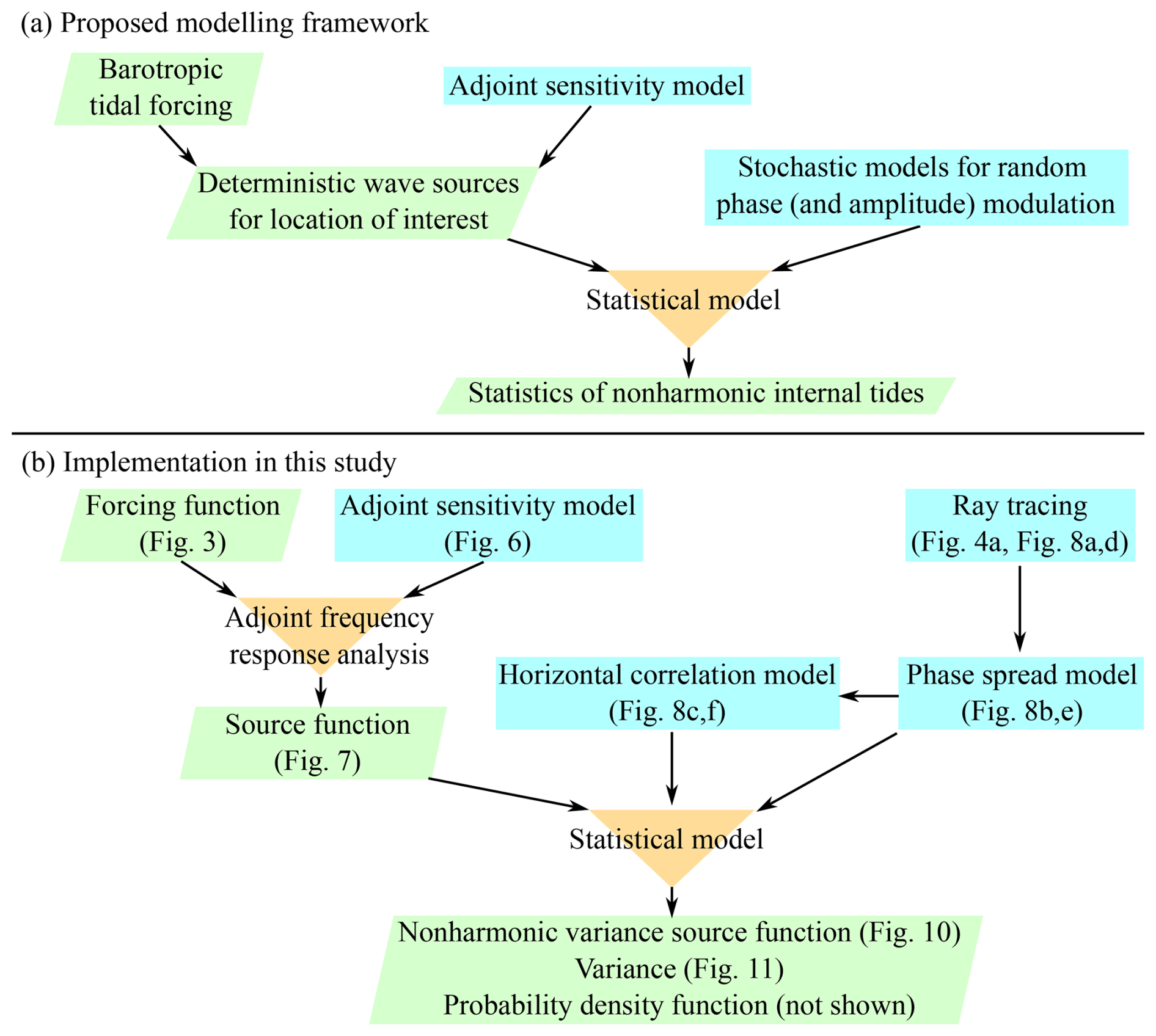
Figure 1 Overview of proposed modelling framework and its implementation in this study. The entire process applies two “filters”: (i) to transform global and deterministic forcing from barotropic to individual baroclinic modes (forcing function) to the corresponding forcing relevant only to a particular observation location (source function) and then (ii) to transform this forcing to a response relevant only to the random component of internal tides (nonharmonic variance source function).

3 Theoretical background

3.1 Statistical model

The basis of the modelling framework proposed in this study is the statistical model developed in Part 1. Only a fraction of the model is needed in Part 2, which primarily considers the variance of nonharmonic internal tides. This section introduces relevant relationships from Part 1 for independent waves and then extends them to correlated waves.

The statistical model in Part 1 considers internal tides with a single vertical-mode structure in a narrow frequency band observed at a fixed observation location and approximates them as a sinusoidal time series that has the deterministic angular frequency ω, the deterministic mean phase lag φ, a random amplitude A, and a random phase-lag deviation Θ. Furthermore, it is assumed that this signal results from the superposition of independent and non-identically distributed N sinusoidal wave components, each of which has the deterministic mean phase lag φ_j, a random amplitude A_j, and a random phase-lag deviation Θ_j. Then, the signal can be expressed as

$$\begin{array}{}\text{(1)}& A{e}^{-i(\mathit{\phi }+\mathrm{\Theta })}{e}^{i\mathit{\omega }t}=\sum _{j=\mathrm{1}}^N{A}_j{e}^{-i\left({\mathit{\phi }}_j+{\mathrm{\Theta }}_j\right)}{e}^{i\mathit{\omega }t},\end{array}$$

where t is time. Unlike Part 1, the mean phase lags are subtracted from the total phase lags to make Θ and Θ_j random variables with zero mean, and only deterministic amplitudes A_j=a_j are hereafter considered for individual wave components. The phase PDF is assumed to be the wrapped normal (or Gaussian) distribution as in Part 1:

$$\begin{array}{}\text{(2)}& f_{{\mathrm{\Theta }}_j}\left({\mathit{\theta }}_j\right)={\displaystyle \frac{\mathrm{1}}{\sqrt{\mathrm{2}\mathit{\pi }}{\mathit{\sigma }}_j}}\sum _{k=-\mathrm{\infty }}^{\mathrm{\infty }}\exp \left(-{\displaystyle \frac{{\left({\mathit{\theta }}_j+\mathrm{2}\mathit{\pi }k\right)}^{\mathrm{2}}}{\mathrm{2}{\mathit{\sigma }}_j^{\mathrm{2}}}}\right),\end{array}$$

where σ_j is the standard deviation of the phase. The wrapped normal distribution is a circular analogue of the Gaussian distribution and defined for any one period of 2π. It approaches the Gaussian distribution in the limit σ_j→0 but approaches the uniform distribution in the limit σ_j→∞. Since harmonic analysis determines harmonic amplitudes and phase lags using the method of least squares, the complex-valued amplitudes (i.e. their magnitudes represent wave amplitudes and their angles represent wave phases as the coefficients of a complex Fourier series) are further decomposed into the expected values and deviations from them:

$$\begin{array}{}\text{(3)}& \begin{array}{rl}A{e}^{-i(\mathit{\phi }+\mathrm{\Theta })}& =r{e}^{-i\mathit{\phi }}+A^{\prime }{e}^{-i(\mathit{\phi }+{\mathrm{\Theta }}^{\prime })}\\ & =\sum _{j=\mathrm{1}}^N\left(r_j{e}^{-i{\mathit{\phi }}_j}+A_j^{\prime }{e}^{-i\left({\mathit{\phi }}_j+{\mathrm{\Theta }}_j^{\prime }\right)}\right).\end{array}\end{array}$$

Here, r_j is the magnitude of the expected complex-valued amplitude on the complex plane, and $A_j^{\prime }$ and ${\mathrm{\Theta }}_j^{\prime }$ are the amplitude and phase lag of the deviation, respectively (see Fig. 2). Note that (r, φ) and (A^′, $\mathit{\phi }+{\mathrm{\Theta }}^{\prime }$) correspond to harmonic and nonharmonic internal tides, respectively. Note also that Θ^′ and ${\mathrm{\Theta }}_j^{\prime }$ are random variables with zero mean unlike Part 1 and that A, A^′, and $A_j^{\prime }$ are random variables even though a_j is deterministic (see Fig. 2 and Part 1). Assuming tentatively that σ_j in Eq. (2) is known and that all the wave components are independent, the expectation and variance of the complex-valued random amplitudes $a_j{e}^{-i({\mathit{\phi }}_j+{\mathrm{\Theta }}_j)}$ are (see Part 1)

$$\begin{array}{}\text{(4a)}& {\displaystyle }E\left(a_j{e}^{-i\left({\mathit{\phi }}_j+{\mathrm{\Theta }}_j\right)}\right)=r_j{e}^{-i{\mathit{\phi }}_j}=a_j{\mathit{\mu }}_j{e}^{-i{\mathit{\phi }}_j},\text{(4b)}& {\displaystyle }\mathrm{Var}\left(a_j{e}^{-i\left({\mathit{\phi }}_j+{\mathrm{\Theta }}_j\right)}\right)=E\left({A_j^{\prime }}^{\mathrm{2}}\right)=a_j^{\mathrm{2}}{\mathit{\varsigma }}_j^{\mathrm{2}},\text{(4c)}& {\displaystyle }{\mathit{\mu }}_j=e^{-{\mathit{\sigma }}_j^{\mathrm{2}}/\mathrm{2}},\text{(4d)}& {\displaystyle }{\mathit{\varsigma }}_j^{\mathrm{2}}=\mathrm{1}-e^{-{\mathit{\sigma }}_j^{\mathrm{2}}}.\end{array}$$

Hereafter, E(⋅) and Var(⋅) denote the expectation and variance, respectively. For complex-valued variables, the variance is defined as $\mathrm{Var}\left(X\right)=E\left(\right(X-E\left(X\right)\left)\right(X-E\left(X\right){)}^{*})$. Hereafter, the superscript * denotes complex conjugate. Then, because of the independence of individual wave components, $E\left({A^{\prime }}^{\mathrm{2}}\right)$ is given by (see Part 1 for justification)

$$\begin{array}{}\text{(5)}& E\left({A^{\prime }}^{\mathrm{2}}\right)=\sum _{j=\mathrm{1}}^{N}E\left({A_j^{\prime }}^{\mathrm{2}}\right).\end{array}$$

Note that $E\left({A^{\prime }}^{\mathrm{2}}\right)$ is the variance of the envelope amplitude of nonharmonic internal tides and is twice the nonharmonic internal-tide variance because the sinusoidal “carrier” wave (i.e. e^iωt in Eq. 1) has the variance of $\mathrm{1}/\mathrm{2}$.

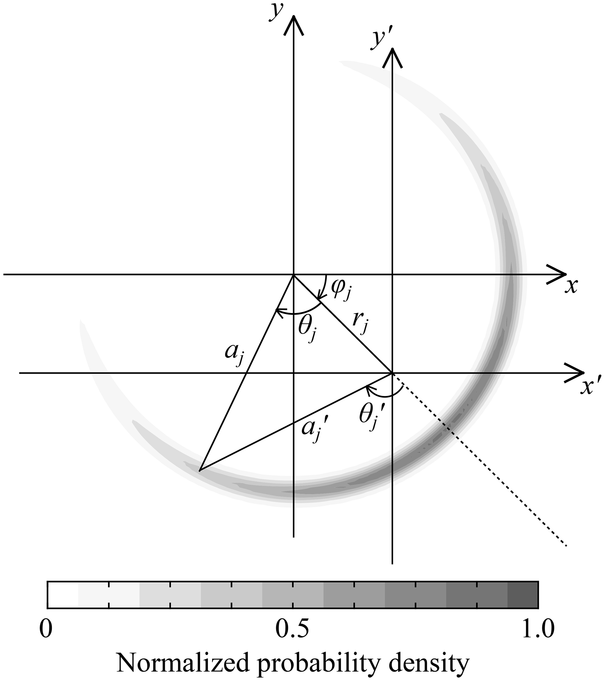
Figure 2 Schematics of variables used in the statistical model and probability density function for individual wave components. x_j+iy_j is the (total) complex-valued amplitude (i.e. its magnitude represents wave amplitude and its angle represents wave phase as the coefficients of complex Fourier series), $x_j^{\prime }+i{y}_j^{\prime }$ is that with zero mean, and angles are positive clockwise because harmonic analysis conventionally uses phase lags. Shading shows the probability density function of a wrapped normal distribution, with a narrow Gaussian amplitude spread to make the shading discernible. Note that a_j is assumed to be constant, but $a_j^{\prime }$ varies because of phase distribution. Note also that (a_j, θ_j) and ($a_j^{\prime }$, ${\mathit{\theta }}_j^{\prime }$) are realizations of (A_j, Θ_j) and ($A_j^{\prime }$, ${\mathrm{\Theta }}_j^{\prime }$) in Eqs. (1) and (3), respectively. For illustration purposes, ${\mathit{\phi }}_j=\mathit{\pi }/\mathrm{4}$ and σ_j=0.3π are used.

The above argument assumes the independence of individual wave components; however, the horizontal correlation of phase modulation along the propagation paths introduces the correlation of wave components arriving from individual sources. To consider the horizontal correlation, we remove the assumption of independent wave components in Eqs. (1) and (3) and calculate the covariance of the ith and jth wave components. Using Eqs. (1), (3), and (4a)–(4d), we get

$$\begin{array}{}\text{(6)}& \mathrm{Cov}\left(A_i^{\prime }{e}^{-i{\mathit{\phi }}_i}{e}^{-i{\mathrm{\Theta }}_i^{\prime }},A_j^{\prime }{e}^{-i{\mathit{\phi }}_j}{e}^{-i{\mathrm{\Theta }}_j^{\prime }}\right)=s_i{\mathit{\varsigma }}_i{R}_{ij}{\mathit{\varsigma }}_j{s}_j^{*},\end{array}$$

where $s_j=a_j{e}^{-i{\mathit{\phi }}_j}$ represents complex-valued pre-modulation wave amplitudes from individual sources (hereafter referred to as “sources”), R_ij is the correlation coefficient of $e^{-i{\mathrm{\Theta }}_i}$ and $e^{-i{\mathrm{\Theta }}_j}$, and the covariance is defined as $\mathrm{Cov}(X,Y)=E\left(\right(X-E\left(X\right)\left)\right(Y-E\left(Y\right){)}^{*})$. Note that ${\mathrm{\Theta }}_j^{\prime }$ does not follow the wrapped normal distribution in Eq. (2), but $A_j^{\prime }{e}^{-i{\mathrm{\Theta }}_j^{\prime }}$ can be expressed in terms of $a_j{e}^{-i{\mathrm{\Theta }}_j}$, μ_j, and ς_j using Eqs. (1), (3), and (4a)–(4d). This yields

$$\begin{array}{}\text{(7)}& R_{ij}={\displaystyle \frac{\mathrm{1}}{{\mathit{\varsigma }}_i{\mathit{\varsigma }}_j}}\left(\exp \left\{-{\displaystyle \frac{\mathrm{1}}{\mathrm{2}}}E\left(\mathrm{\Delta }{\mathrm{\Theta }}^{\mathrm{2}}\right)\right\}-{\mathit{\mu }}_i{\mathit{\mu }}_j\right),\end{array}$$

where $\mathrm{\Delta }\mathrm{\Theta }={\mathrm{\Theta }}_i-{\mathrm{\Theta }}_j$. Since the difference of correlated wrapped normal variables is a wrapped normal variable, the expectation in the above equation is obtained using

$$\begin{array}{}\text{(8)}& E\left(e^{-i\mathrm{\Delta }\mathrm{\Theta }}\right)=\exp \left\{-{\displaystyle \frac{\mathrm{1}}{\mathrm{2}}}E\left(\mathrm{\Delta }{\mathrm{\Theta }}^{\mathrm{2}}\right)\right\},\end{array}$$

which is the same relationship as for the normally distributed phase (Colosi and Munk, 2006; Geoffroy and Nycander, 2022). Note that this relationship makes the correlation coefficients R_ij real-valued, although the original variable, e^−iΔΘ, is complex-valued. To derive this convenient relationship, the definition of Θ_j is changed from Part 1 to have zero mean. To proceed, Colosi and Munk (2006) and Geoffroy and Nycander (2022) assumed the correlation functions of Θ_i and Θ_j, but we aim to express E(ΔΘ²) as a function of the variance and correlation length of phase speed. This is done by stochastic modelling, as described in Sect. 3.5.

The correlation coefficients in Eq. (7) can be used to convert correlated sources (e.g. from hydrodynamic modelling) to effectively independent sources that can be used in the statistical model. To do so, we write the complex-valued amplitude of nonharmonic internal tides $A^{\prime }{e}^{-i(\mathit{\phi }+{\mathrm{\Theta }}^{\prime })}$ in Eq. (3) in two ways. On the one hand, we assume that the waves from individual sources $s_j=a_j{e}^{-i{\mathit{\phi }}_j}$ are later modulated by horizontally correlated random phase shifts, yielding

$$\begin{array}{}\text{(9)}& A^{\prime }{e}^{-i(\mathit{\phi }+{\mathrm{\Theta }}^{\prime })}={\mathit{s}}_{\mathrm{phys}}^T\mathbf{\Sigma }{\mathit{n}}_{\mathrm{corr}}.\end{array}$$

Here, s is the vector containing s_j, and Σ is a diagonal matrix whose diagonal components are ς_j defined in Eq. (4d). Hereafter, the superscript T denotes transpose. The above form is chosen so that the vector n, with its components ${\mathit{\varsigma }}_j^{-\mathrm{1}}(e^{-i{\mathrm{\Theta }}_j}-E(e^{-i{\mathrm{\Theta }}_j}\left)\right)$, is a vector containing random variables with zero mean and unit variance (but not Gaussian) on the complex plane. The subscript “phys” emphasizes that the variable is calculated based on physics (in this study, by the adjoint frequency response analysis introduced in Sect. 3.2), and the subscript “corr” emphasizes horizontally correlated random variables. The statistical model, on the other hand, requires independent random variables:

$$\begin{array}{}\text{(10)}& A^{\prime }{e}^{-i(\mathit{\phi }+{\mathrm{\Theta }}^{\prime })}={\mathit{s}}_{\mathrm{stat}}^T\mathbf{\Sigma }\mathit{n},\end{array}$$

where the vector s_stat contains the amplitudes of independent sources. Now, we may assume that two random vectors are related as ${\mathit{n}}_{\mathrm{corr}}={\mathbf{R}}^{\mathrm{1}/\mathrm{2}}\mathit{n}$, where $\mathbf{R}={\mathbf{R}}^{\mathrm{1}/\mathrm{2}}{\mathbf{R}}^{T/\mathrm{2}}$ is the horizontal correlation coefficient matrix whose components are given by Eq. (7). Note that n is complex-valued, but R is real-valued because of Eq. (8). Assuming tentatively that ${\mathbf{R}}^{\mathrm{1}/\mathrm{2}}$ is known, the comparison of the above two equations shows

$$\begin{array}{}\text{(11)}& {\mathit{s}}_{\mathrm{stat}}={\mathbf{\Sigma }}^{-\mathrm{1}}{\mathbf{R}}^{T/\mathrm{2}}\mathbf{\Sigma }{\mathit{s}}_{\mathrm{phys}}.\end{array}$$

We use this relationship to convert horizontally correlated sources calculated based on physics to effectively independent sources that can be used in the statistical model. Then, considering Eqs. (4b) and (5) in a matrix form and $E\left({\mathit{n}}^{*}{\mathit{n}}^T\right)=\mathbf{I}$, we get

$$\begin{array}{}\text{(12)}& \begin{array}{rl}E\left({A^{\prime }}^{\mathrm{2}}\right)& ={\mathit{s}}_{\mathrm{stat}}^H{\mathbf{\Sigma }}^{\mathrm{2}}{\mathit{s}}_{\mathrm{stat}}\\ & ={\left({\mathbf{R}}^{T/\mathrm{2}}\mathbf{\Sigma }{\mathit{s}}_{\mathrm{phys}}\right)}^H{\mathbf{R}}^{T/\mathrm{2}}\mathbf{\Sigma }{\mathit{s}}_{\mathrm{phys}}.\end{array}\end{array}$$

Hereafter, the superscript H denotes conjugate transpose. Note that the (i, j) component in the summation corresponds to Eq. (6). Appendix C provides detailed points regarding the above treatment of horizontal correlation using ${\mathbf{R}}^{\mathrm{1}/\mathrm{2}}$.

The continuous version of Eq. (12) is useful in this study. The equation divided by 2 can be written as

$$\begin{array}{}\text{(13)}& \begin{array}{rl}{\displaystyle \frac{\mathrm{1}}{\mathrm{2}}}E\left({A^{\prime }}^{\mathrm{2}}\right)& =\int s_{\mathrm{nh}}\left(\overrightarrow{x}\right)\mathrm{d}\overrightarrow{x}\\ & ={\displaystyle \frac{\mathrm{1}}{\mathrm{2}}}\int {\left(\int R^{\mathrm{1}/\mathrm{2}}({\overrightarrow{x}}^{\prime },\overrightarrow{x})\mathit{\varsigma }\left({\overrightarrow{x}}^{\prime }\right)s\left({\overrightarrow{x}}^{\prime }\right)\mathrm{d}{\overrightarrow{x}}^{\prime }\right)}^{*}\\ & \times \left(\int R^{\mathrm{1}/\mathrm{2}}({\overrightarrow{x}}^{\prime },\overrightarrow{x})\mathit{\varsigma }\left({\overrightarrow{x}}^{\prime }\right)s\left({\overrightarrow{x}}^{\prime }\right)\mathrm{d}{\overrightarrow{x}}^{\prime }\right)\mathrm{d}\overrightarrow{x}.\end{array}\end{array}$$

The variables $s\left(\overrightarrow{x}\right)$ and $s_{\mathrm{nh}}\left(\overrightarrow{x}\right)$ are hereafter referred to as the “source function” and “nonharmonic variance source function” (more correctly source density function), and $s\left(\overrightarrow{x}\right)$, $\mathit{\varsigma }\left(\overrightarrow{x}\right)$, and $R^{\mathrm{1}/\mathrm{2}}({\overrightarrow{x}}^{\prime },\overrightarrow{x})$ are the continuous versions of s_phys, Σ, and ${\mathbf{R}}^{T/\mathrm{2}}$, respectively. (Note that Σ is a diagonal matrix.) The factor $\mathrm{1}/\mathrm{2}$ is multiplied in the above equation so that the integral of s_nh corresponds to the variance of a nonharmonic internal-tide time series from observations or numerical modelling, rather than the variance of the envelope amplitude. The above expression shows that, because the horizontal integral of s_nh yields the total nonharmonic internal-tide variance, s_nh can be mapped to identify their important source regions. Also, a regional integral of s_nh yields the contribution of that region to the total variance. Although not shown in this paper, s_nh can also be used to calculate PDFs using the theory in Part 1. (However, note that s_nh is nonunique within the correlation length of phase modulation because ${\mathbf{R}}^{T/\mathrm{2}}$ in Eq. (12) or $R^{\mathrm{1}/\mathrm{2}}({\overrightarrow{x}}^{\prime },\overrightarrow{x})$ in Eq. (13) is nonunique, as explained in Appendix C.)

3.2 Adjoint sensitivity modelling and calculation of deterministic internal-tide sources

In order to calculate the deterministic sources of internal tides for a fixed observation location, we use a combination of adjoint sensitivity modelling and the frequency response analysis from Fourier theory, referred to as “adjoint frequency response analysis” in this study. A brief summary and the major output of the method are described below. Appendix D provides an overview of the adjoint method, which is often used in inverse problems, and the details of the adjoint frequency response analysis.

The basic idea of the adjoint frequency response analysis is as follows. Since internal tides are linear waves and their major generation forces are deterministic as a first approximation, the forcing and so-called impulse response function can be used to obtain spatially and temporally varying internal waves excited by forcing at a particular location and time. A problem converse to this yields spatially and temporally varying sources of internal waves at a particular location and time (including both harmonic and nonharmonic components) by considering the forcing and the so-called adjoint sensitivity (or the Green's function; e.g. Bennett, 2002). These methods can be extended to sinusoidal internal tides using the Fourier transform.

The application of the adjoint frequency response analysis to internal tides under realistic stratification and bathymetry requires a linear numerical hydrodynamic model and its adjoint. In this paper, we use a linear hydrodynamic model based on vertical-mode decomposition in Shimizu (2011) and Shimizu (2019). The formulation employs horizontally varying vertical modes that are calculated using local water depths and stratification in order to include the effects of steep slopes (for approximately linear waves). More details are described in Appendix B. An advantage of this formulation is that it yields the evolutionary equations analogous to the shallow water equations with explicit forcing functions from barotropic tides to individual baroclinic modes. As an example, the forcing function from the barotropic to VM1 M₂ tide is shown in Fig. 3.

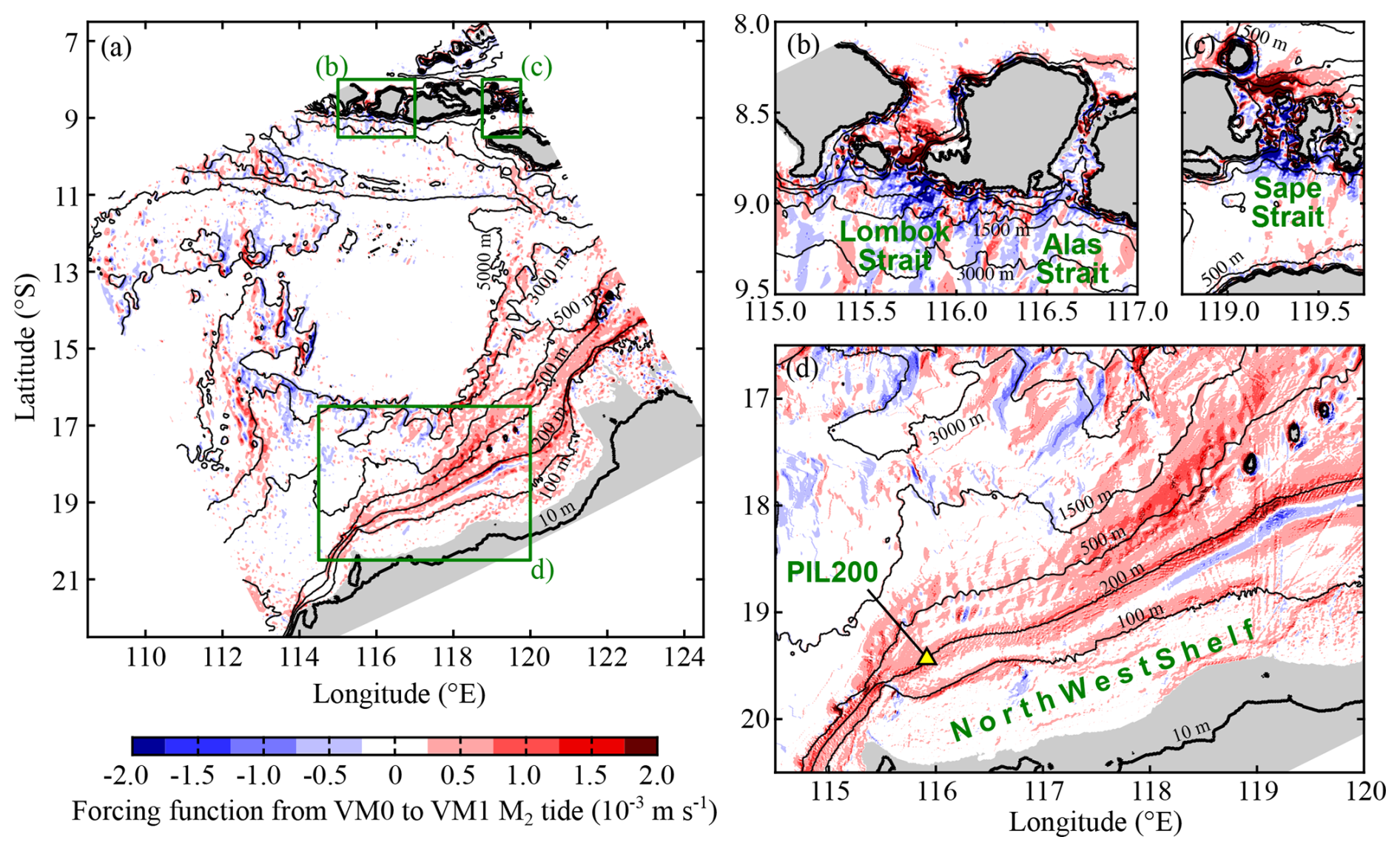
Figure 3 Forcing function from the barotropic-mode (VM0) to vertical-mode-one (VM1) M₂ tide (at zero Greenwich phase lag). It corresponds to $\stackrel{\mathrm{̃}}{f}$ in Eq. (14). Panel (a) shows the whole model domain, and panels (b)–(d) show zoomed views of the green boxes in (a). Grey shading shows regions where VM1 celerity is less than 0.1 m s⁻¹.

If only one baroclinic mode is considered in the hydrodynamic model, the adjoint frequency response analysis allows us to write the complex-valued internal-tide amplitude as

$$\begin{array}{}\text{(14)}& a{e}^{-i\mathit{\phi }}=\int s\left(\overrightarrow{x}\right)\mathrm{d}\overrightarrow{x}=\int \mathrm{2}{\stackrel{\mathrm{̃}}{\mathit{\lambda }}}^{*}\left(\overrightarrow{x}\right)\stackrel{\mathrm{̃}}{f}\left(\overrightarrow{x}\right)\mathrm{d}\overrightarrow{x},\end{array}$$

where a and φ are the pre-modulation amplitude and phase of isopycnal displacement due to the baroclinic mode of interest at the location of interest, respectively. The variable $\stackrel{\mathrm{̃}}{f}$ is the forcing function from the barotropic tidal currents to the baroclinic mode, and $\stackrel{\mathrm{̃}}{\mathit{\lambda }}$ is the adjoint frequency response function of ae^−iφ to $\stackrel{\mathrm{̃}}{f}$ at other locations, calculated by the adjoint of the linear hydrodynamic model. These variables are defined in Appendix D. The function $s\left(\overrightarrow{x}\right)$ is the source function appearing in Eq. (13). The middle expression shows that, because the horizontal integral of the source function yields the complex-valued amplitude ae^−iφ, s can be mapped to identify important source regions. The right expression shows that the adjoint frequency response function $\stackrel{\mathrm{̃}}{\mathit{\lambda }}$ acts as a transfer function from the forcing function $\stackrel{\mathrm{̃}}{f}$, which provides forcing in a global sense, to the source function s; this provides forcing relevant to the location of interest. The maps of $\stackrel{\mathrm{̃}}{f}$ and $\stackrel{\mathrm{̃}}{\mathit{\lambda }}$ can be used to identify regions where forcing and dynamic response are large. The important advantage of the source function in this study is that it provides horizontally distributed sources of internal tides observed at a fixed location so that different phase statistics can be assigned to different sources.

It is also convenient to write Eq. (14) in a discretized form. The equation can be written as

$$\begin{array}{}\text{(15)}& a{e}^{-i\mathit{\phi }}=\sum _{j=\mathrm{1}}^N{s}_j=\sum _{j=\mathrm{1}}^N{a}_j{e}^{-i{\mathit{\phi }}_j},\end{array}$$

where s_j represents the discretized version of $s\left(\overrightarrow{x}\right)$. The variables $s_j=a_j{e}^{-i{\mathit{\phi }}_j}$ are sought-after wave sources corresponding to s_phys in Eq. (11).

3.3 Stochastic differential equations for phase modelling

To develop stochastic models of phase statistics, we consider waves with a constant frequency that arrive at an observation location after travelling through regions of random phase-speed variability. Following Zaron and Egbert (2014) and the analysis in Appendix A, the random phase deviation along the wave propagation path between a source located at ${\overrightarrow{x}}_j$ and the observation location (say, jth path) can be calculated considering the variation of the total wave phase $\mathrm{d}\left(\mathrm{phase}\right)=\mathit{\omega }(\mathrm{d}t-c_j^{-\mathrm{1}}\mathrm{d}{\mathit{\xi }}_j)-\mathrm{d}({\mathit{\phi }}_j+{\mathit{\theta }}_j)$ and that of the phase speed c_j, where ξ_j is the coordinate along the path. (Note that θ_j is the stochastic version of Θ_j in Eq. 1.) Some examples of wave propagation paths are shown in Fig. 4a. To introduce random components in the phase lag and phase speed, we write $c_j={\stackrel{\mathrm{‾}}{c}}_j+c_j^{\prime }$ and assume that φ_j and ${\stackrel{\mathrm{‾}}{c}}_j$ are the respective mean components, and θ_j and $c_j^{\prime }$ are the respective stochastic components with zero mean. Assuming $\left|c_j^{\prime }\right|\ll {\stackrel{\mathrm{‾}}{c}}_j$ and following the constant mean phase ($\mathrm{d}{\mathit{\xi }}_j={\stackrel{\mathrm{‾}}{c}}_j\mathrm{d}t$), the deviation of total phase due to $c_j^{\prime }$ or θ_j is given by $c_j^{\prime }{\stackrel{\mathrm{‾}}{c}}_j^{-\mathrm{2}}\mathit{\omega }\mathrm{d}{\mathit{\xi }}_j$ and −dθ_j, respectively. This yields (see Appendix A for alternative derivation)

$$\begin{array}{}\text{(16)}& \mathrm{d}{\mathit{\theta }}_j=-{\displaystyle \frac{\mathit{\omega }{c}_j^{\prime }}{{\stackrel{\mathrm{‾}}{c}}_j}}\mathrm{d}t,\end{array}$$

where time t is used as the independent variable because it is a convenient common coordinate variable for multiple paths.

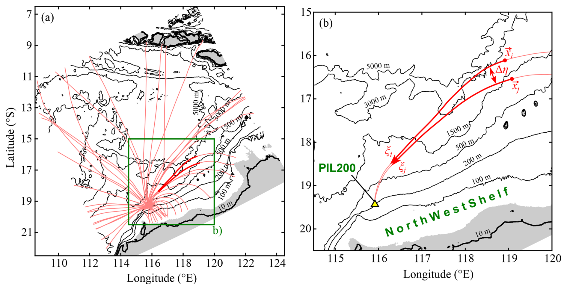
Figure 4 An example of ray paths for the vertical-mode-one (VM1) M₂ internal tide and schematics of variables used in cross-path phase difference modelling. Pink lines indicate ray paths. Panel (a) shows the whole model domain, and panel (b) shows a zoomed view of the green box in (a) for two example ray paths. Grey shading shows regions where VM1 celerity is less than 0.1 m s⁻¹.

Since θ_j and $c_j^{\prime }$ are stochastic variables, Eq. (16) is a stochastic differential equation. Stochastic differential equations are commonly forced by white Gaussian noise, but it is undesirable to assume $c_j^{\prime }$ is white noise because $c_j^{\prime }$ certainly has spatial correlation. A common “trick” used to deal with correlated noise is to introduce an additional stochastic equation driven by white noise, which yields the desired correlation function (see e.g. Särkkä and Solin, 2019, chap. 12.3). For example, we may assume that $c_j^{\prime }$ follows

$$\begin{array}{}\text{(17)}& \mathrm{d}{c}_j^{\prime }=-{\displaystyle \frac{{\stackrel{\mathrm{‾}}{c}}_j}{L_C}}{c}_j^{\prime }\mathrm{d}t+\sqrt{{\displaystyle \frac{{\stackrel{\mathrm{‾}}{c}}_j}{L_C}}}\mathrm{d}{b}_j,\end{array}$$

where L_C is the e-folding correlation length of $c_j^{\prime }$. The variable b_j is a random variable called Brownian motion (see e.g. Särkkä and Solin, 2019, chap. 4.1). Intuitively, the above equation can be formally divided by dt and $\mathrm{d}{b}_j/\mathrm{d}t$ regarded as white noise, although this view is mathematically incorrect in general.

The stochastic phase models used in this study are developed by considering covariance equations associated with the above two stochastic differential equations. The details of the derivation are given in Appendix E, and only the final equations used for the modelling are provided in the following two sections. Note that we need to integrate only ordinary differential equations in this study because the covariance equations are ordinary differential equations, although the formulation is based on stochastic differential equations.

3.4 Stochastic phase spread model

To model the phase variance ${\mathit{\sigma }}_j^{\mathrm{2}}$ in Eqs. (4c)–(4d), we consider Eqs. (16) and (17) along a single wave propagation path. The evolutionary equations of the covariance between $c_j^{\prime }$ and θ_j, P_cθ, and that between θ_j and θ_j, P_θθ, are given by

$$\begin{array}{}\text{(18a)}& {\displaystyle }& {\displaystyle \frac{\mathrm{d}{P}_{c\mathit{\theta }}}{\mathrm{d}t}}=-{\displaystyle \frac{\stackrel{\mathrm{‾}}{c}}{L_C}}{P}_{c\mathit{\theta }}-{\displaystyle \frac{\mathit{\omega }}{\stackrel{\mathrm{‾}}{c}}}{\mathit{\sigma }}_C^{\mathrm{2}},\text{(18b)}& {\displaystyle }& {\displaystyle \frac{\mathrm{d}{P}_{\mathit{\theta }\mathit{\theta }}}{\mathrm{d}t}}=-\mathrm{2}{\displaystyle \frac{\mathit{\omega }}{\stackrel{\mathrm{‾}}{c}}}{P}_{c\mathit{\theta }},\end{array}$$

where ${\mathit{\sigma }}_C^{\mathrm{2}}$ is the phase-speed variance, and the subscript j is suppressed for brevity. If $\stackrel{\mathrm{‾}}{c}$ and L_C remain constant, the solution under the initial condition $P_{c\mathit{\theta }}=P_{\mathit{\theta }\mathit{\theta }}=\mathrm{0}$ at t=0 is

$$\begin{array}{}\text{(19)}& P_{\mathit{\theta }\mathit{\theta }}=\mathrm{2}{\displaystyle \frac{{\mathit{\sigma }}_C^{\mathrm{2}}}{{\stackrel{\mathrm{‾}}{c}}^{\mathrm{2}}}}{\left({\displaystyle \frac{\mathit{\omega }{L}_{\mathrm{C}}}{\stackrel{\mathrm{‾}}{c}}}\right)}^{\mathrm{2}}\left({\displaystyle \frac{\stackrel{\mathrm{‾}}{c}t}{L_C}}-\mathrm{1}+e^{-\stackrel{\mathrm{‾}}{c}t/L_C}\right).\end{array}$$

This agrees with Eq. (12) in Zaron and Egbert (2014) if the correlation function of c^′ is assumed to be exponential (Eq. E5). Note that it is essential to consider the phase-speed correlation length L_C because a small correlation length makes phase-speed variability less efficient in inducing phase variance.

The straightforward approach for solving Eqs. (18a)–(18b) is to integrate the equations from a source location to the observation location; however, this approach is computationally inefficient because it needs separate (forward) integration from each source location along the same path. Alternatively, we can exploit the adjoint method described in Appendix D. The adjoint sensitivity of P_θθ at the observation location to [P_cθP_θθ]^T at other locations can be calculated by integrating the equations adjoint to Eqs. (18a)–(18b) once, backwards in time from the observation location. Then, P_θθ can be calculated as the convolution of the adjoint sensitivity and the forcing (i.e. the ${\mathit{\sigma }}_C^{\mathrm{2}}$ term in Eq. 18a) along the path. The resultant phase variance P_θθ, which grows with distance from the observation location, is used as the phase variance ${\mathit{\sigma }}_j^{\mathrm{2}}$ in the statistical model. Note that P_θθ can grow without a limit, but this does not cause any problem because the wrapped normal distribution in Eq. (2) can be used with arbitrarily large phase spread σ_j.

3.5 Stochastic cross-path phase difference model

We now consider the calculation of the variance of the phase difference E(ΔΘ²) in Eq. (7). Note that full evaluation of E(ΔΘ²) is difficult for relatively large problems because E(ΔΘ²) depends on pairs of two source locations, which vary over the area considered (e.g. model domain). For this reason, a number of approximations are introduced in the theory in this section and in numerical methods later in Sect. 4.4. To simplify the calculation of phase difference ΔΘ, we consider ΔΘ only in the cross-path direction in this section.

The modelling of cross-path phase difference ΔΘ is done by considering Eqs. (16) and (17) along two wave propagation paths passing through the same observation location and by calculating the phase difference $\mathrm{\Delta }\mathit{\theta }={\mathit{\theta }}_i-{\mathit{\theta }}_j$ (Δθ is the stochastic version of ΔΘ in Eq. 7). In this section and Appendix E, the subscripts i and j indicate variables along the ith and jth paths, respectively. We take into account the variability of the mean phase speed $\stackrel{\mathrm{‾}}{c}$ and the phase-speed correlation length L_C along the propagation paths but neglect their cross-path variability. The evolutionary equations of the covariance between $c_i^{\prime }$ and Δθ, $P_{c_i\mathrm{\Delta }\mathit{\theta }}$, that of $c_j^{\prime }$ and Δθ, $P_{c_j\mathrm{\Delta }\mathit{\theta }}$, and that of Δθ and Δθ, P_ΔθΔθ, are given by

$$\begin{array}{}\text{(20a)}& {\displaystyle }& {\displaystyle \frac{\mathrm{d}{P}_{c_i\mathrm{\Delta }\mathit{\theta }}}{\mathrm{d}t}}=-{\displaystyle \frac{\stackrel{\mathrm{‾}}{c}}{L_C}}{P}_{c_i\mathrm{\Delta }\mathit{\theta }}-{\displaystyle \frac{\mathit{\omega }}{\stackrel{\mathrm{‾}}{c}}}{\mathit{\sigma }}_C^{\mathrm{2}}\left(\mathrm{1}-R_{\mathit{\eta }}\left({\displaystyle \frac{\left|\mathrm{\Delta }\mathit{\eta }\right|}{l}}\right)\right),\text{(20b)}& {\displaystyle }& {\displaystyle \frac{\mathrm{d}{P}_{c_j\mathrm{\Delta }\mathit{\theta }}}{\mathrm{d}t}}=-{\displaystyle \frac{\stackrel{\mathrm{‾}}{c}}{L_C}}{P}_{c_j\mathrm{\Delta }\mathit{\theta }}+{\displaystyle \frac{\mathit{\omega }}{\stackrel{\mathrm{‾}}{c}}}{\mathit{\sigma }}_C^{\mathrm{2}}\left(\mathrm{1}-R_{\mathit{\eta }}\left({\displaystyle \frac{\left|\mathrm{\Delta }\mathit{\eta }\right|}{l}}\right)\right),\text{(20c)}& {\displaystyle }& {\displaystyle \frac{\mathrm{d}{P}_{\mathrm{\Delta }\mathit{\theta }\mathrm{\Delta }\mathit{\theta }}}{\mathrm{d}t}}=-\mathrm{2}{\displaystyle \frac{\mathit{\omega }}{\stackrel{\mathrm{‾}}{c}}}\left(P_{c_i\mathrm{\Delta }\mathit{\theta }}-P_{c_j\mathrm{\Delta }\mathit{\theta }}\right),\end{array}$$

where

$$\begin{array}{}\text{(21)}& R_{\mathit{\eta }}\left({\displaystyle \frac{\left|\mathrm{\Delta }\mathit{\eta }\right|}{l}}\right)={\displaystyle \frac{F\left(\right|\mathrm{\Delta }\mathit{\eta }|/l)}{\mathrm{1}+F^{\mathrm{2}}\left(\right|\mathrm{\Delta }\mathit{\eta }|/l)}}\end{array}$$

is the cross-path correlation function of phase speed, Δη is the cross-path distance,

$$\begin{array}{}\text{(22a)}& {\displaystyle }& {\displaystyle }F\left(\right|\mathrm{\Delta }\mathit{\eta }|/l)=e^{-\left|\mathrm{\Delta }\mathit{\eta }\right|/l},\text{(22b)}& {\displaystyle }& {\displaystyle }l=\mathrm{2}{\mathit{\pi }}^{-\mathrm{1}}{L}_C,\end{array}$$

and l is the cross-path correlation length. Generally, P_ΔθΔθ needs to be calculated numerically. However, if $\stackrel{\mathrm{‾}}{c}$, L_C, and $\left|\mathrm{\Delta }\mathit{\eta }\right|/l$ remain constant, the comparison of Eqs. (20a)–(20c) and (18a)–(18b) leads to the explicit solution

$$\begin{array}{}\text{(23)}& P_{\mathrm{\Delta }\mathit{\theta }\mathrm{\Delta }\mathit{\theta }}=\mathrm{2}{P}_{\mathit{\theta }\mathit{\theta }}\left(\mathrm{1}-R_{\mathit{\eta }}\left(\right|\mathrm{\Delta }\mathit{\eta }|/l)\right),\end{array}$$

where P_θθ is given by Eq. (19). (It may appear odd to assume constant $\left|\mathrm{\Delta }\mathit{\eta }\right|/l$ because $\left|\mathrm{\Delta }\mathit{\eta }\right|$ certainly varies; however, an empirical relationship is introduced later in Sect. 4.4 to account for the variation.) This shows that the cross-path correlation length of Δθ depends on the phase-speed correlation length L_C through Eqs. (22a)–(22b). This is important because L_C can be estimated from observations or hydrodynamic modelling more easily than the correlation length of phase difference Δθ.

Similar to Eqs. (18a)–(18b), Eqs. (20a)–(20c) can be solved using the adjoint method explained in Appendix D, and the resultant variance P_ΔθΔθ corresponds to E(ΔΘ²) in Eq. (7). However, note that the analysis has been simplified substantially by the assumptions introduced above. In particular, note that P_ΔθΔθ=0 at Δη=0, which implies R_ij=1 in Eq. (7) because Eqs. (20a)–(20c) neglect along-path correlation. To take into account the effects of along-path correlation, an empirical adjustment is introduced later in Sect. 4.4.

4 Methods

4.1 Application to VM1 semidiurnal internal tides at PIL200 location

To illustrate application of the proposed model suite, we took vertical-mode-one (VM1) semidiurnal internal tides at the PIL200 mooring site (115.915° E, 19.435° S, ≈200 m deep) of the Australian Integrated Marine Observing System on the Australian North West Shelf (Figs. 3 and 4) as an example. Part 1 analysed the nonharmonic VM1 to vertical-mode-four (VM4) diurnal, semidiurnal, and quarter-diurnal internal tides in the observations.

In the model suite, we included the four major semidiurnal tidal constituents (M₂, S₂, K₂, and N₂) and four lowest baroclinic modes (VM1–VM4). Figure 5 shows a flowchart for the application of the proposed model suite to multiple tidal constituents and vertical modes. Forcings from the major constituents were considered separately, assuming that the nonharmonic internal-tide variance (and the associated statistics) is calculated for a sufficiently long time series. Since it was impractical to separate nonharmonic internal tides into constituents in the PIL200 observations (Part 1), the resultant variance, $E\left({A^{\prime }}^{\mathrm{2}}\right)/\mathrm{2}$ in Eq. (13), and the nonharmonic variance source functions from individual constituents were summed to obtain the total for semidiurnal internal tides. It may sound confusing to include multiple baroclinic modes for modelling VM1 internal tides at the PIL200 location. This is required because barotropic forcing excites not only VM1 but also higher modes, which can be converted to VM1 by topographic interaction before arriving at the PIL200 location (see Fig. 5). To distinguish overall barotropic forcing to VM1 internal tides at the PIL200 location from barotropic forcing to individual baroclinic modes in the intermediate process, the latter is hereafter referred to as, for example, “barotropic-to-VM2” or “VM0-to-VM2” forcing.

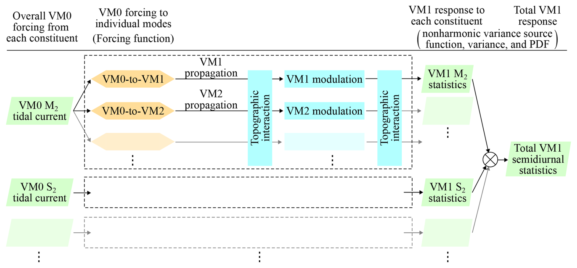
Figure 5 Flowchart for application of the proposed model suite to multiple tidal constituents and vertical modes. Abbreviations are PDF: probability density function, VM0: barotropic mode, VM1: vertical mode one, and VM2: vertical mode two.

4.2 Adjoint frequency response function and source function modelling

In the hydrodynamic modelling, we considered linear hydrostatic internal tides under climatological stratification without background currents. Note that mesoscale oceanic variability is intentionally omitted because its effects are represented by random phase-speed variability in the stochastic models (see Appendix A for the justification of this treatment). A sinusoidal periodic motion was assumed (as in Eq. D7) in the governing equations (Eqs. B3a–B3c in without the nonlinear terms) so that the hydrodynamic model directly calculates the adjoint frequency response function ($\stackrel{\mathrm{̃}}{\mathit{\lambda }}$ in Eq. 14). The frequency response function was calculated for complex-valued VM1 isopycnal displacement amplitude at the PIL200 location (i.e. ae^−iφ in Eq. 14), whose magnitude is scaled to have the value of extreme (maximum or minimum) displacement within the water column.

Details of the hydrodynamic model set-up are as follows. The model grid encompass most of the Australian North West Shelf and part of the Lesser Sunda Islands in Indonesia (Fig. 3a). The horizontal coordinates are oriented in the cross-shelf (NNW–SSE) and along-shelf (SSW–NNE) directions at the PIL200 location. The horizontal grid size is 0.01°. The model extent and grid resolution are not ideal but were limited by available computational resources. The four lowest baroclinic modes (VM1–VM4) are included in the calculation. Vertical modes are calculated using the 2019 version of GEBCO bathymetry (GEBCO, 2019) and stratification from the 2018 version of World Ocean Atlas annual climatology over the 2005–2017 period (Locarnini et al., 2018; Zweng et al., 2018). TEOS-10 (McDougall and Barker, 2011) is used to calculate density. The model includes horizontally varying linear bottom friction, which is calculated using the (nondimensional) quadratic bottom drag coefficient of 10⁻³ and the barotropic tidal current speed from the TPXO9-atlas version 5 (updated from Egbert and Erofeeva, 2002). Since the grid resolution is not sufficiently high to resolve internal tides in regions with shallow water depths or weak stratification, we exclude regions where the celerity of each (nth) vertical mode c_n is less than 0.1 m s⁻¹, which roughly corresponds to four grid points per wavelength for semidiurnal tides. (In this study, the term “celerity” is deliberately used for the propagation speed of non-rotating, long, linear gravity waves with one of the vertical-mode structures, which differs from the phase speed of internal tides.) The Flather open boundary condition (Flather, 1976; see also Blayo and Debreu, 2005) is applied to individual vertical modes at the open boundaries. The adjoint frequency response function was calculated separately for the M₂, S₂, K₂, and N₂ tidal frequencies.

The source function ($s\left(\overrightarrow{x}\right)$ in Eq. 14) was calculated from the adjoint frequency response function for the four lowest baroclinic modes and barotropic currents from the TPXO9-atlas for the four major semidiurnal constituents. This provided 16 source functions in total.

4.3 Ray tracing and phase spread modelling

The phase variance P_θθ was calculated based on Eqs. (18a)–(18b), but it required finding wave propagation paths from the PIL200 location. We took the simplest approach and calculated the propagation paths by standard ray theory (e.g. Lighthill, 1978, chap. 4.5), but applying it backwards in time. The initial location is the PIL200 location and the initial angles are in 0.1 and 1° intervals for rays propagating towards offshore and onshore, respectively. Additional rays are used to ensure that some rays propagate into the southern part of the major straits in the Lesser Sunda Islands, such as the Lombok Strait. Figure 4a shows about $\mathrm{1}/\mathrm{30}$ of the calculated ray paths as examples.

The standard ray equations and the equations adjoint to Eqs. (18a)–(18b) were integrated backwards in time using the fourth-order Runge–Kutta method for VM1 to VM4 semidiurnal internal tides. The time steps are 300, 450, 600, and 900 s for VM1, VM2, VM3, and VM4, respectively. In the calculation, the along-path variability of water depth, phase speed, and Coriolis parameter are taken into account. Since the results were insensitive to small frequency differences among the major semidiurnal constituents, the M₂ frequency was used in the modelling.

The phase-speed variance ${\mathit{\sigma }}_C^{\mathrm{2}}$ in the model was chosen based on the PIL200 observations, which yielded ${\mathit{\sigma }}_{C,\mathrm{PIL}\mathrm{200}}^{\mathrm{2}}\approx \mathrm{12}$, 9.5, 8.2, and $\mathrm{8.2}\times {\mathrm{10}}^{-\mathrm{3}}$ m² s⁻² for VM1, VM2, VM3, and VM4 semidiurnal internal tides, respectively (Appendix F). Although the observations were made on the continental shelf at ≈ 200 m water depth, the phase-speed variance of VM1 is not unreasonable for deep ocean. For example, previous numerical modelling (Zaron and Egbert, 2014; Buijsman et al., 2017) suggests ${\mathit{\sigma }}_C/\stackrel{\mathrm{‾}}{c}$ = 1 %–3 % in deep ocean for VM1 semidiurnal internal tides. Since these values include only low-frequency components, they are likely to be underestimates for ${\mathit{\sigma }}_C^{\mathrm{2}}$, which needs to include all frequency components as explained in Appendix F. So, ${\mathit{\sigma }}_C^{\mathrm{2}}\approx \mathrm{1.2}\times {\mathrm{10}}^{-\mathrm{2}}$ m² s⁻², which yields ${\mathit{\sigma }}_C/\stackrel{\mathrm{‾}}{c}\approx \mathrm{3.6}$ % assuming $\stackrel{\mathrm{‾}}{c}=\mathrm{3}$ m s⁻¹, appears to be roughly the upper limit of the current estimate of ${\mathit{\sigma }}_C^{\mathrm{2}}$ for deep ocean. For higher modes, phase-speed variance appeared to be unavailable except those from Appendix F. These facts suggest that horizontally constant phase-speed variance is not a bad assumption, so we chose ${\mathit{\sigma }}_C^{\mathrm{2}}$ by scaling ${\mathit{\sigma }}_{C,\mathrm{PIL}\mathrm{200}}^{\mathrm{2}}$ as

$$\begin{array}{}\text{(24)}& {\mathit{\sigma }}_C^{\mathrm{2}}={\mathit{\alpha }}_C{\mathit{\sigma }}_{C,\mathrm{PIL}\mathrm{200}}^{\mathrm{2}},\end{array}$$

where α_C is a model parameter. This choice is also a simple and convenient way to show the dependence of the results on ${\mathit{\sigma }}_C^{\mathrm{2}}$. We used α_C varying between 0.4 and 1.0. As already explained, α_C=1.0 is the estimate for the PIL200 location and appears to be roughly the current upper limit for deep ocean. The choice α_C=0.4 (${\mathit{\sigma }}_C/\stackrel{\mathrm{‾}}{c}\approx \mathrm{2.3}$ %) is about the middle range of the current estimate for deep ocean, but it would be a substantial underestimate for shallow water. We chose the middle of these likely upper and lower limits, α_C=0.7, as a reference value.

Regarding the correlation length of phase speed L_C, we assumed L_C to be proportional to the Rossby radius of deformation $R_d={\stackrel{\mathrm{‾}}{c}}_{\mathrm{1}}/f$:

$$\begin{array}{}\text{(25)}& L_C={\mathit{\alpha }}_L{R}_d,\end{array}$$

where f is the Coriolis parameter, and α_L is a model parameter. This choice was made for two reasons. First, R_d is a common length scale used for mesoscale oceanic variability. Second, L_C is expected to vary substantially between continental shelves and deep ocean, and the mean VM1 celerity ${\stackrel{\mathrm{‾}}{c}}_{\mathrm{1}}$ in the expression of R_d conveniently reflects at least some part of this variability. Note that the same ${\stackrel{\mathrm{‾}}{c}}_{\mathrm{1}}$ is used to calculate L_C for all the higher modes, considering that the phase-speed modulations of all vertical modes are caused by the same oceanic variability. The phase-speed correlation length appears to be rarely evaluated, but Zaron and Egbert (2014) showed that the correlation length was about 3 times R_d around Hawaii. This value might be affected by the smoothing scale of the reanalysis product used in their study and is larger than the typical radius of mesoscale eddies for the latitude (e.g. Klocker and Abernathey, 2014). However, phase-speed correlation could be affected by processes that have a length scale larger than eddies (e.g. Buijsman et al., 2017). Since the typical eddy radius is roughly R_d for the latitude range of the model domain (e.g. Klocker and Abernathey, 2014), the realistic parameter range is α_L≳1. We chose the middle-ground value of α_L=2 as a reference value. Note that the wavelength of VM1 semidiurnal internal tides is about 1–2 times R_d in the modelled region.

After the ray-based calculation, the travel time and phase variance P_θθ along the ray paths were horizontally interpolated to obtain gridded results using a Gaussian kernel. This interpolated P_θθ was used as ${\mathit{\sigma }}_j^{\mathrm{2}}$ in the statistical model.

4.4 Horizontal phase correlation modelling

The horizontal correlation coefficient matrix R was implemented as a diffusion operator following Weaver and Courtier (2001), which is a numerical technique commonly used in data assimilation (see e.g. Bennett, 2002, chap. 3.1.6). This is because, although R could be calculated in principle using Eqs. (7) and (20a)–(20c), it was prohibitive to store the whole R on computer memory in practice. The method approximates the correlation function as Gaussian and requires the correlation lengths at individual grid points, which are equivalent to the standard deviation of the Gaussian function (i.e. impulse response solution to the diffusion equation). Since Eqs. (20a)–(20c) calculate the variance of the cross-path phase difference for different cross-path distance $\left|\mathrm{\Delta }\mathit{\eta }\right|$, Eqs. (7) and (20a)–(20c) yield only the cross-path correlation length σ_η, and the along-path correlation length σ_ξ is still missing. In this study, an empirical relationship between σ_η and σ_ξ was introduced, and equivalent isotropic diffusion was assumed for simplicity. Then, the phase correlation modelling requires the equivalent isotropic correlation length of phase modulation at each grid point σ_r calculated from P_ΔθΔθ in Eqs. (20a)–(20c).

To determine σ_r, we assume

$$\begin{array}{}\text{(26)}& \left|\mathrm{\Delta }\mathit{\eta }\right|={\mathit{\alpha }}_r^{-\mathrm{1}}\mathrm{\Delta }r\end{array}$$

in Eqs. (20a)–(20c), where Δr is the distance between the sources, and α_r is an empirical parameter whose meaning is explained shortly. This assumption has the advantage that P_ΔθΔθ could be integrated (backwards in time) for various values of Δr together with the ray tracing and integration of P_θθ, and the results can be gridded in the same way. Substituting the resultant P_ΔθΔθ into E(ΔΘ²) in Eq. (7) yields the horizontal correlation function at each grid point R(Δr). (In Eq. 7, μ_i=μ_j and ς_i=ς_j are assumed.) Then, by approximating the first peak of R(Δr) as Gaussian, we get

$$\begin{array}{}\text{(27)}& R\left(\mathrm{\Delta }r\right)\approx \exp \left(-{\displaystyle \frac{\mathrm{\Delta }{r}^{\mathrm{2}}}{\mathrm{2}{\mathit{\alpha }}_r^{\mathrm{2}}{\mathit{\sigma }}_{\mathit{\eta }}^{\mathrm{2}}}}\right).\end{array}$$

The empirical factor α_r represents two effects: anisotropy of the horizontal correlation of phase modulation and the along-path variation of cross-path distance. Typical values of α_r for these effects are considered in the following.

To estimate α_r for anisotropic phase correlation, we tentatively regard R_ij in Eq. (7) as the correlation function R(Δξ,Δη) (Δξ is a lag distance in the along-path direction) and compare its integral scale with that of the equivalent isotropic correlation function R(Δr). Assuming that the correlation functions are Gaussian and equating the integrals, we get

$$\begin{array}{}\text{(28)}& \begin{array}{rl}\underset{-\mathrm{\infty }}{\overset{\mathrm{\infty }}{\int }}\underset{-\mathrm{\infty }}{\overset{\mathrm{\infty }}{\int }}& \exp \left(-{\displaystyle \frac{\mathrm{\Delta }{\mathit{\xi }}^{\mathrm{2}}}{\mathrm{2}{\mathit{\sigma }}_{\mathit{\xi }}^{\mathrm{2}}}}-{\displaystyle \frac{\mathrm{\Delta }{\mathit{\eta }}^{\mathrm{2}}}{\mathrm{2}{\mathit{\sigma }}_{\mathit{\eta }}^{\mathrm{2}}}}\right)\mathrm{d}\mathrm{\Delta }\mathit{\xi }\mathrm{d}\mathrm{\Delta }\mathit{\eta }\\ & \approx \mathrm{2}\mathit{\pi }\underset{\mathrm{0}}{\overset{\mathrm{\infty }}{\int }}\mathrm{\Delta }r\exp \left(-{\displaystyle \frac{\mathrm{\Delta }{r}^{\mathrm{2}}}{\mathrm{2}{\mathit{\sigma }}_r^{\mathrm{2}}}}\right)\mathrm{d}\mathrm{\Delta }r,\end{array}\end{array}$$

where σ_ξ is the unknown standard deviation in the along-path direction. This yields the relationship of the integral scales,

$$\begin{array}{}\text{(29)}& {\mathit{\sigma }}_{\mathit{\xi }}{\mathit{\sigma }}_{\mathit{\eta }}\approx {\mathit{\sigma }}_r^{\mathrm{2}}.\end{array}$$

The comparison of Eqs. (27)–(29) shows that ${\mathit{\alpha }}_r=\sqrt{{\mathit{\sigma }}_{\mathit{\xi }}/{\mathit{\sigma }}_{\mathit{\eta }}}$, and α_r=1 for the isotropic correlation function (σ_ξ=σ_η). Note the relatively weak dependence of α_r on σ_ξ. For example, the correlation function is highly anisotropic for σ_ξ=9σ_η, but it yields α_r=3.

To estimate α_r for the along-path variation of cross-path distance, we consider the linear variation of cross-path distance $\left|\mathrm{\Delta }\mathit{\eta }\right|$ between the observation location and source locations. Since the distance between the sources is Δr, an intuitive value for average $\left|\mathrm{\Delta }\mathit{\eta }\right|$ over the paths is α_r=2. However, note that ray tracing suggests large along-path variability of $\left|\mathrm{\Delta }\mathit{\eta }\right|$ (Fig. 4a).

Based on the above consideration, the equivalent isotropic correlation length of phase modulation σ_r was calculated from Eqs. (7) and (20a)–(20c), and (26) as follows. Considering both the anisotropy of the phase correlation and the along-path variation of cross-path distance, α_r between 1 and 5 appears to be reasonable. We chose the middle of these likely upper and lower limits, α_r=3, as a reference value. Using Eq. (26) with a chosen α_r, P_ΔθΔθ from Eqs. (20a)–(20c) was substituted into Eq. (7) to calculate the correlation coefficient for a different source distance Δr. This yielded the isotropic correlation function R(Δr). Since σ_r is required for the diffusion operator method, the Gaussian shape was fitted to the first peak of the correlation function where R(Δr)>0.5 by the least-squares method, and the resultant standard deviation is used as σ_r in the diffusion operator method.

In addition to σ_r, the diffusion operator method also requires normalization factors that impose R_ii≈1 after applying the diffusion operator (i.e. the matrix Λ in Weaver and Courtier, 2001). The normalization factors are calculated by the ensemble method explained in Weaver and Courtier (2001). We used 200 ensemble members, which correspond to the standard error of 5 % in the normalization of R.

As in the ray tracing and phase spread modelling, σ_r and the normalization factors were calculated separately for the four lowest baroclinic modes using the M₂ frequency. The frequency differences among semidiurnal constituents were neglected.

4.5 Calculation of nonharmonic variance source function

The nonharmonic variance source function was calculated for each constituent from Eq. (12) using s_phys from the source function, Σ calculated from the phase variance $P_{\mathit{\theta }\mathit{\theta }}={\mathit{\sigma }}_j^{\mathrm{2}}$, and R implemented as a diffusion operator with the equivalent isotropic correlation length of phase modulation σ_r; however, it required one more assumption because it was not obvious which phase spread and phase correlation should be applied to each source function. For example, if higher modes are directly excited by barotropic forcing and converted to VM1 near the sources, and then the VM1 internal tides propagate to the observation location (follow VM0-to-VM2 forcing, left-hand-side “Topographic interaction”, and then VM1 propagation in Fig. 5), the phase spread and correlation lengths for VM1 should be applied to the source functions for higher modes because the phases are modulated as VM1 internal tides. However, if higher modes are directly excited by barotropic forcing, propagate as higher modes, and are then converted to VM1 near the observation location (follow VM0-to-VM2 forcing, VM2 propagation, right-hand-side “Topographic interaction”, and then VM1 propagation in Fig. 5), the phase spread and correlation lengths for higher modes should be applied to the source functions of respective higher modes. The latter scenario is assumed in this study because the continental slope near the PIL200 location induces strong topographic interaction between VM1 and higher modes, as shown later.

5 Results

5.1 Adjoint frequency response function

The adjoint frequency response function ($\stackrel{\mathrm{̃}}{\mathit{\lambda }}$ in Eq. 14) of VM1-induced isopycnal displacement at the PIL200 location to the barotropic (VM0)-to-VM1 forcing qualitatively shows a pattern of internal waves spreading from a point source but affected by topography-induced variation of the propagation speed (Fig. 6a). For internal-wave signals propagating offshore, wave spreading gradually reduces the magnitudes. By the time the signals reach the Indonesian archipelago, the magnitudes are reduced by a factor of more than 10. For internal-wave signals propagating towards the Australian coast, the wavelengths decrease rapidly because shallower water depths and weaker stratification reduce the propagation speed. The signals disappear on the shelf shallower than 100 m, partly because of bottom friction and partly because the grid resolution gradually becomes insufficient to adequately resolve internal tides there. This numerical dissipation does not change the overall results of this study because the shallow shelf has mild slopes and hence no important sources of internal tides at the PIL200 location.

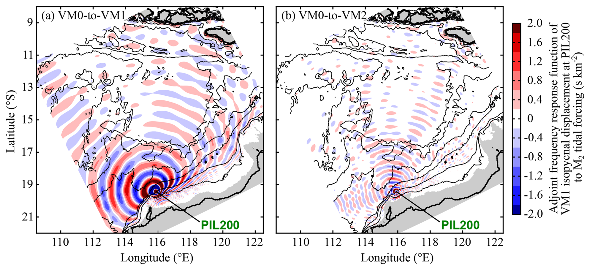
Figure 6 Adjoint frequency response function of vertical-mode-one (VM1)-induced isopycnal displacement at the PIL200 location to M₂ tidal forcing at other locations (at zero Greenwich phase lag). It corresponds to $\stackrel{\mathrm{̃}}{\mathit{\lambda }}$ in Eq. (14). (a) Barotropic-mode (VM0) to VM1 forcing and (b) VM0 to vertical-mode-two (VM2) forcing. Black lines show isobaths at 10, 100, 200, 500, 1500, 3000, and 5000 m water depths. Grey shading shows regions where celerity is less than 0.1 m s⁻¹.

The adjoint frequency response function to the VM0-to-VM2 forcing also shows a pattern of internal waves spreading from a point source (Fig. 6b). The magnitudes are smaller than the VM1 signals because the VM2 (and other higher-mode) signals result from the topographic conversion of VM1 signals on the continental slope. The shorter wavelength shows that the signals are propagating as a free VM2 internal-wave signal, at least as a first approximation. These features justify our choice of applying the phase spread and horizontal phase correlation for VM2 to the VM2 source function (Sect. 4.5). This observation is significant because the spatial pattern would be very different if the topographic conversion occurred near the sources or if VM2 signals resulted from a directly forced response rather than a free-wave response. Additionally, these different scenarios affect which phase spread and horizontal phase correlation should be applied to the VM2 (and higher-mode) source function.

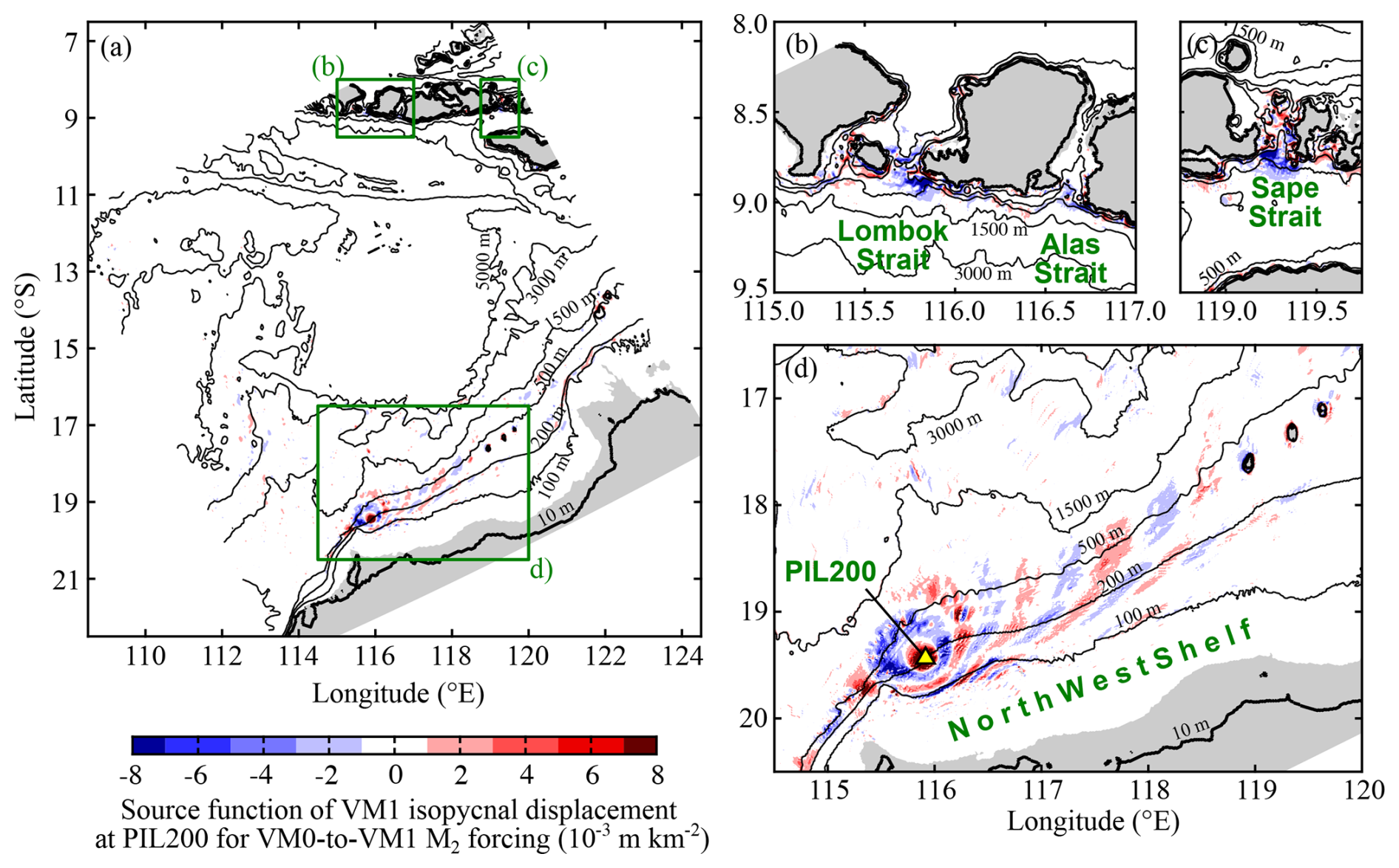
Figure 7 Source function of vertical-mode-one (VM1)-induced isopycnal displacement at the PIL200 location for barotropic (VM0)-to-VM1 M₂ forcing (at zero Greenwich phase lag). It corresponds to s in Eq. (14). Panel (a) shows the whole model domain, and panels (b)–(d) show zoomed views of the green boxes in (a). Grey shading shows regions where VM1 celerity is less than 0.1 m s⁻¹.

5.2 Source function

The source function ($s\left(\overrightarrow{x}\right)$ in Eq. 14) was calculated simply by multiplying the forcing function (Fig. 3) and the complex conjugate of the adjoint frequency response function (Fig. 6). Figure 7 shows the source function of the VM1 M₂ internal tide at the PIL200 location as an example. It shows alternating signs at the wavelength of the VM1 M₂ internal tide. Physically, it means, for example, that the internal tides generated at half a wavelength away from the PIL200 location and then propagated there have the opposite phase from those locally and currently generated at the location. So, these waves tend to cancel each other, and the opposite signs in the source function reflect this wave cancelling. Although the adjoint frequency response function decays with distance (Fig. 6a), remote locations with strong barotropic tides and/or steep bottom slopes can be sources as strong as those near the observation location. For example, the magnitudes of the source function in the straits of the Indonesian archipelago, which are well-known source regions of internal tides, are comparable to those on the Australian shelf.

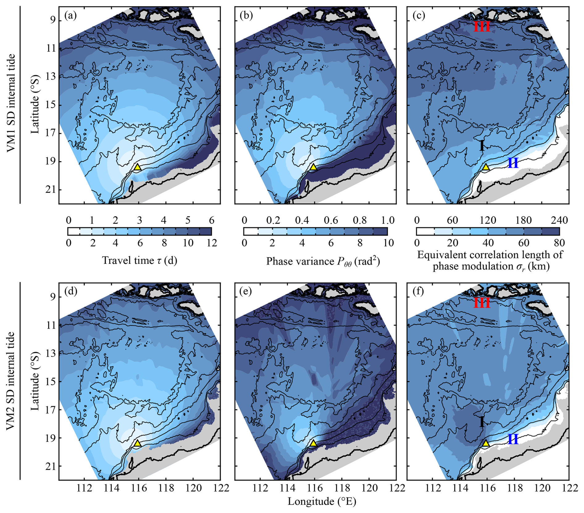
Figure 8 Maps of variables related to the phase modulation of a semidiurnal (SD) internal tide at the PIL200 location in the reference case: (α_C, α_L, α_r) = (0.7, 2, 3). Left, middle, and right panels show the travel time, phase variance, and equivalent isotropic correlation length of phase modulation, respectively. Upper and lower panels are for vertical mode one (VM1) and mode two (VM2), respectively. Note the different scales for upper and lower panels. Roman numerals in panels (c, f) show locations where correlation functions are shown in Fig. 9. Yellow triangles indicate the PIL200 location. Black lines show isobaths at 10, 100, 200, 500, 1500, 3000, and 5000 m water depths. Grey shading shows regions where celerity is less than 0.1 m s⁻¹.

5.3 Phase spread

VM1 internal tides from most of the model domain except the Australian shelf are only partially random (Fig. 8b). The travel time τ for VM1 semidiurnal internal tides calculated by ray theory increases roughly radially from the PIL200 location (Fig. 8a), which agrees with the adjoint sensitivity (Fig. 6a). A clear exception is the Australian shelf where τ grows quickly because of small group velocity. The phase variance $P_{\mathit{\theta }\mathit{\theta }}={\mathit{\sigma }}_j^{\mathrm{2}}$ also increases roughly radially, but the rate of increase is faster on the shelf because the phase-speed variance ${\mathit{\sigma }}_C^{\mathrm{2}}$ relative to the squared mean phase speed ${\stackrel{\mathrm{‾}}{c}}^{\mathrm{2}}$ is much larger there (Fig. 8b). Note that σ_j>1 is a convenient threshold for random sources (see Eq. 4d; also Fig. 2d in Part 1 for illustration).

Unlike VM1, VM2 internal tides are mostly random (Fig. 8e). This is partly because the phase-speed variance ${\mathit{\sigma }}_C^{\mathrm{2}}$ relative to the squared mean phase speed ${\stackrel{\mathrm{‾}}{c}}^{\mathrm{2}}$ is larger for VM2 than VM1, so the rate of increase of phase variance is higher. Another reason is that VM2 internal tides have about twice the travel time compare to VM1, and hence VM2 has more time to be affected by random oceanic variability (Fig. 8d).

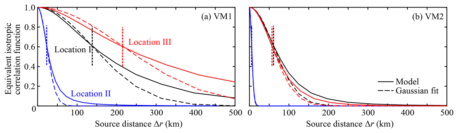
Figure 9 Examples of the equivalent isotropic correlation function of phase modulation at locations I, II, and III indicated in Fig. 8c and f. (a) Vertical mode 1 (VM1) and (b) mode 2 (VM2). Dotted vertical lines indicate standard deviations determined by a least-squares fit of the Gaussian function, which is used as the correlation length σ_r for the diffusion operator method by Weaver and Courtier (2001).

5.4 Horizontal correlation of phase modulation

Since the diffusion operator method by Weaver and Courtier (2001) was used to represent the horizontal correlation of phase modulation, the equivalent isotropic phase correlation length σ_r characterizes the horizontal correlation. It shows an order-of-magnitude variability between the deep ocean and continental shelf for VM1 (Fig. 8c) and tends to have a magnitude comparable to but smaller than α_rL_C over a large part of the model domain. The reason for this can be seen by considering Eqs. (7) and (23) in the limit of small $P_{\mathit{\theta }\mathit{\theta }}={\mathit{\sigma }}_j^{\mathrm{2}}$, which suggests the length scale 2π⁻¹α_rL_C. For example, the gradual increase in σ_r towards north reflects the latitudinal variation of the Rossby radius of deformation, which is assumed to be proportional to L_C. The small σ_r on the continental shelf results from small celerity (and hence small Rossby radius of deformation). The modelled equivalent isotropic correlation functions at three contrasting locations are shown in Fig. 9a. The correlation function generally has a broader tail than the Gaussian function. The modelled and fitted correlation functions agree around the correlation value of 0.6, which corresponds to σ_r (standard deviation of the Gaussian function).

The equivalent isotropic correlation length σ_r for VM2 is substantially smaller than VM1 (Fig. 8f) and does not have the rough relationship with L_C, although the same L_C is used for VM1 and VM2. This is because the phase variance $P_{\mathit{\theta }\mathit{\theta }}={\mathit{\sigma }}_j^{\mathrm{2}}$ is much larger for VM2 than VM1 (Fig. 8b and e), which makes the gradient of P_ΔθΔθ around $\left|\mathrm{\Delta }\mathit{\eta }\right|/l\ll \mathrm{1}$ larger (see Eq. 23) and the decay of the exponential function in Eq. (7) faster. As a result, the latitudinal variation does not exist for VM2, but the order-of-magnitude variability between the deep ocean and continental shelf remains. Figure 9b shows that the modelled and fitted correlation functions agree well for correlation values larger than 0.6 for VM2.

5.5 Contributions of different source regions, vertical modes, and tidal constituents

The results of the model suite provide the contributions of different source regions, vertical modes, and tidal constituents to the modelled nonharmonic internal tides and their dependence on the model parameters. We look at different contributions using the reference case (α_C, α_L, α_r) = (0.7, 2, 3) as an example in this section and then the parameter dependence in the next section.

Table 1 Contributions of different regions to nonharmonic vertical-mode-one (VM1) semidiurnal internal-tide variance (in m²) at the PIL200 location in the reference case: (α_C, α_L, α_r) = (0.7, 2, 3). Variance is based on time series of extreme (maximum or minimum) isopycnal displacement within the water column. Abbreviations for the regions are LOC: local region near the PIL200 location shallower than 1500 m, NWS: Australian North West Shelf region excluding the LOC region, LAS: region around Lombok and Alas straits, SS: region around Sape Strait, and IND: the rest of the model domain, mostly the deep Indian Ocean. These regions are shown in Fig. 10.

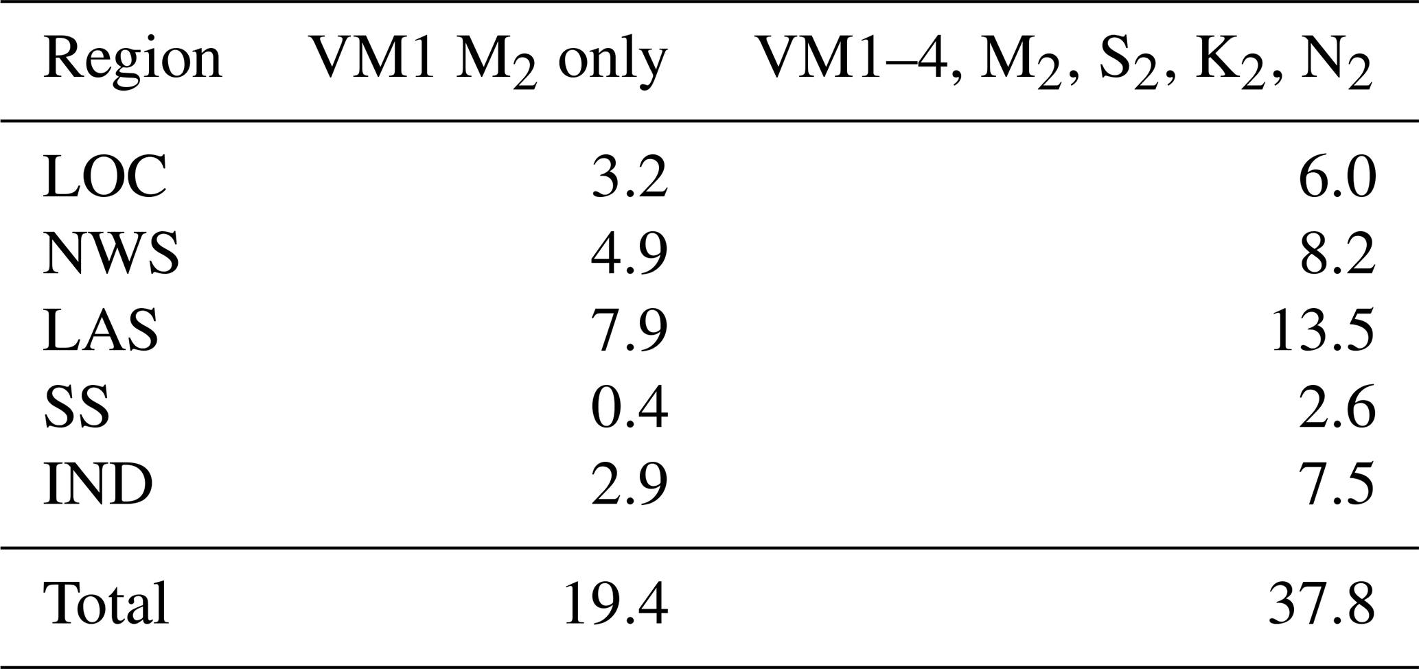
The total modelled nonharmonic VM1 semidiurnal internal-tide variance is 38 m² in the reference case compared to the observed variance of 45±12 m² (confidence interval based on twice the standard error). As explained in Sect. 4.2, the variance is calculated based on VM1-induced extreme (maximum or minimum) isopycnal displacements within the water column. The modelled variance can be converted to vertically integrated potential energies in J m⁻² by multiplying by 7.6 and the variance of surface displacements in m² by multiplying by $\mathrm{7.1}\times {\mathrm{10}}^{-\mathrm{7}}$ (without seasonal variation).

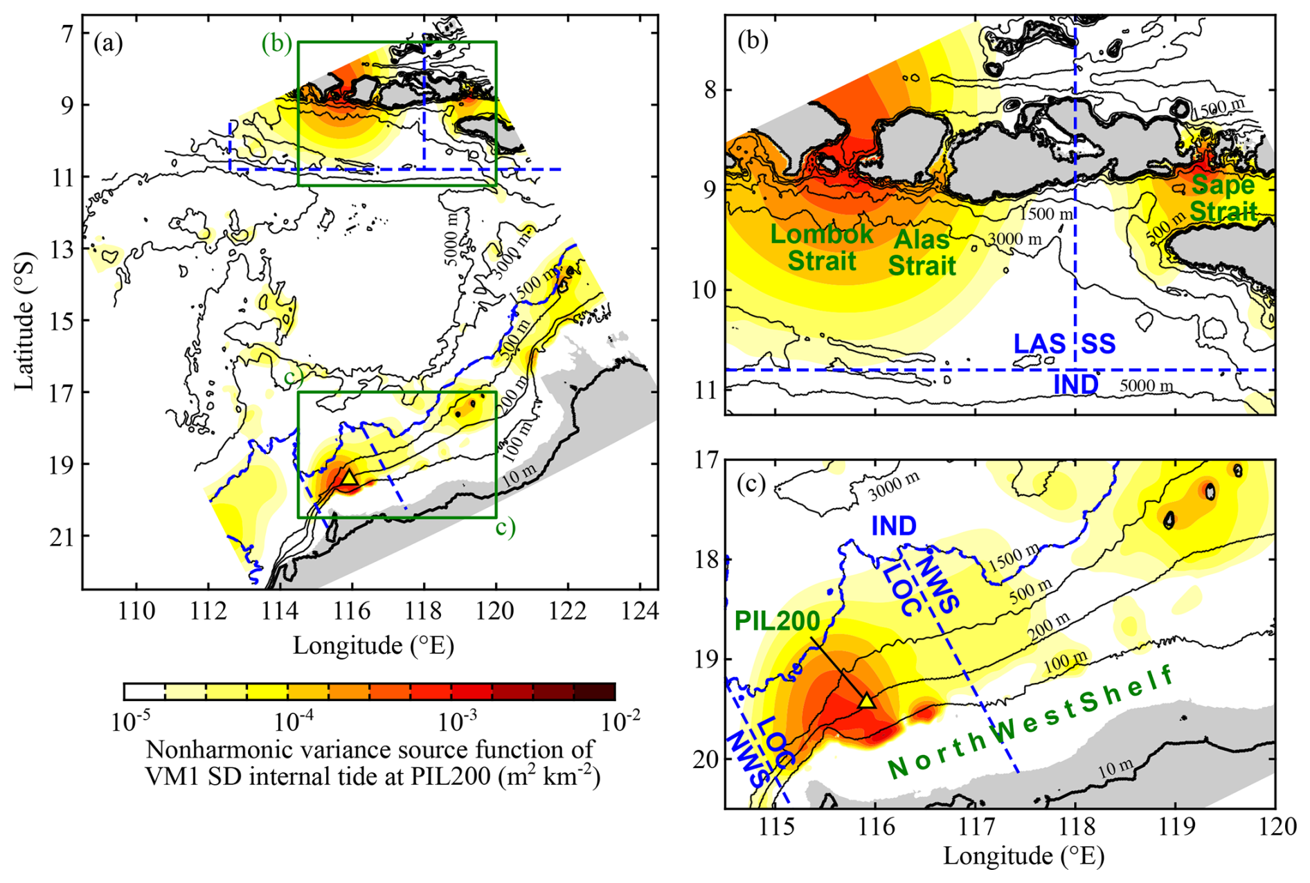
Figure 10 Nonharmonic variance source function of isopycnal displacement induced by the nonharmonic vertical-mode-one (VM1) semidiurnal (SD) internal tide at the PIL200 location in the reference case: (α_C, α_L, α_r) = (0.7, 2, 3). The lowest four baroclinic modes and four major semidiurnal constituents are included. Panel (a) shows the whole model domain, and panels (b)–(d) show zoomed views of the green boxes in (a). Grey shading shows regions where VM1 celerity is less than 0.1 m s⁻¹.

The contributions of different regions are shown in Fig. 10 as a map of nonharmonic variance source function and in Table 1 as regionally integrated contributions. The following regions are arbitrarily chosen for illustration purposes. The LOC region is the local region near the PIL200 location on the Australian North West Shelf shallower than 1500 m, and the NWS region is the Australian shelf region excluding the LOC region. The LAS and SS regions cover the Lombok and Alas straits and Sape Strait, respectively. The IND region is the rest of the model domain, mostly the deep Indian Ocean. These regions are indicated by dashed blue lines in Fig. 10. Figure 10 shows that important source regions are the Australian shelf and the straits in the Indonesian archipelago. The nonharmonic variance source function appears much smoother than the source function in Fig. 7 because the diffusion operator that approximates the correlation coefficient matrix R is applied, and the phase correlation lengths are relatively large (Fig. 8c and f). The horizontal scale of the nonharmonic variance source function is smaller than the correlation length for VM1 (Fig. 8c). This is partly because higher modes have smaller correlation lengths (Fig. 8f) and partly because the diffusion operator averages the opposing contributions from the source function (e.g. red and blue patches in Fig. 7) when the correlation length is comparable to or larger than the wavelength. However, note that the locations of sources in the nonharmonic variance source function are uncertain within the phase correlation length in the current approach, as explained in Appendix C. This is why contributions from relatively large regions are compared in Table 1.

Table 1 shows that remote regions are more important sources of the nonharmonic internal tides than local sources. For example, the contributions of the Australian shelf are smaller than those of the Indonesian straits, and the local contribution on the Australian shelf is smaller than the rest of the shelf. This is because remote sources can be as strong as local sources before phase modulation (Fig. 7), and it takes time for random phase-speed variability to make internal tides nonharmonic (Fig. 8b and e). Although the magnitude of the nonharmonic variance source function in the deep ocean (IND region) is nearly 2 orders of magnitude smaller than the peak values in the major sources (Fig. 10), Table 1 shows that the overall contribution is substantial because it occupies a much larger area than the other regions. Figure 10 also suggests that, although we used a relatively large model domain for available computational resources, the current modelling is likely to have missed remote sources. It is likely that at least a few m² of variance is missing from the deep Indian Ocean to the west of the model domain.

Table 2 shows the contributions of different vertical modes and tidal constituents to the modelled variance. The tabular entry for VM2 and M₂ represents, for example, the contribution of the VM2 internal tide that is excited by the M₂ barotropic forcing and then converted to VM1 before arriving at the PIL200 location. Regarding the contributions of different vertical modes, the model results show that VM1 contributes about $\mathrm{3}/\mathrm{4}$ of the total variance, and the contributions decrease with increasing mode number. Regarding the contributions of different tidal constituents, M₂ and S₂ forcings contribute roughly $\mathrm{3}/\mathrm{4}$ and $\mathrm{1}/\mathrm{4}$ of the total variance, respectively. The contributions of K₂ and N₂ are small (1.8 m²). The VM1 directly forced by M₂ alone contributes roughly half of the total variance. So, VM1 and M₂ are dominant, but focusing only on VM1 and M₂ would cause substantial underestimation of the nonharmonic semidiurnal internal-tide variance in this case.

Table 2 Contributions of different vertical modes (VMs) and tidal constituents to nonharmonic VM1 semidiurnal internal-tide variance (in m²) at the PIL200 location in the reference case: (α_C, α_L, α_r) = (0.7, 2, 3). Variance is based on time series of extreme (maximum or minimum) isopycnal displacement within the water column.

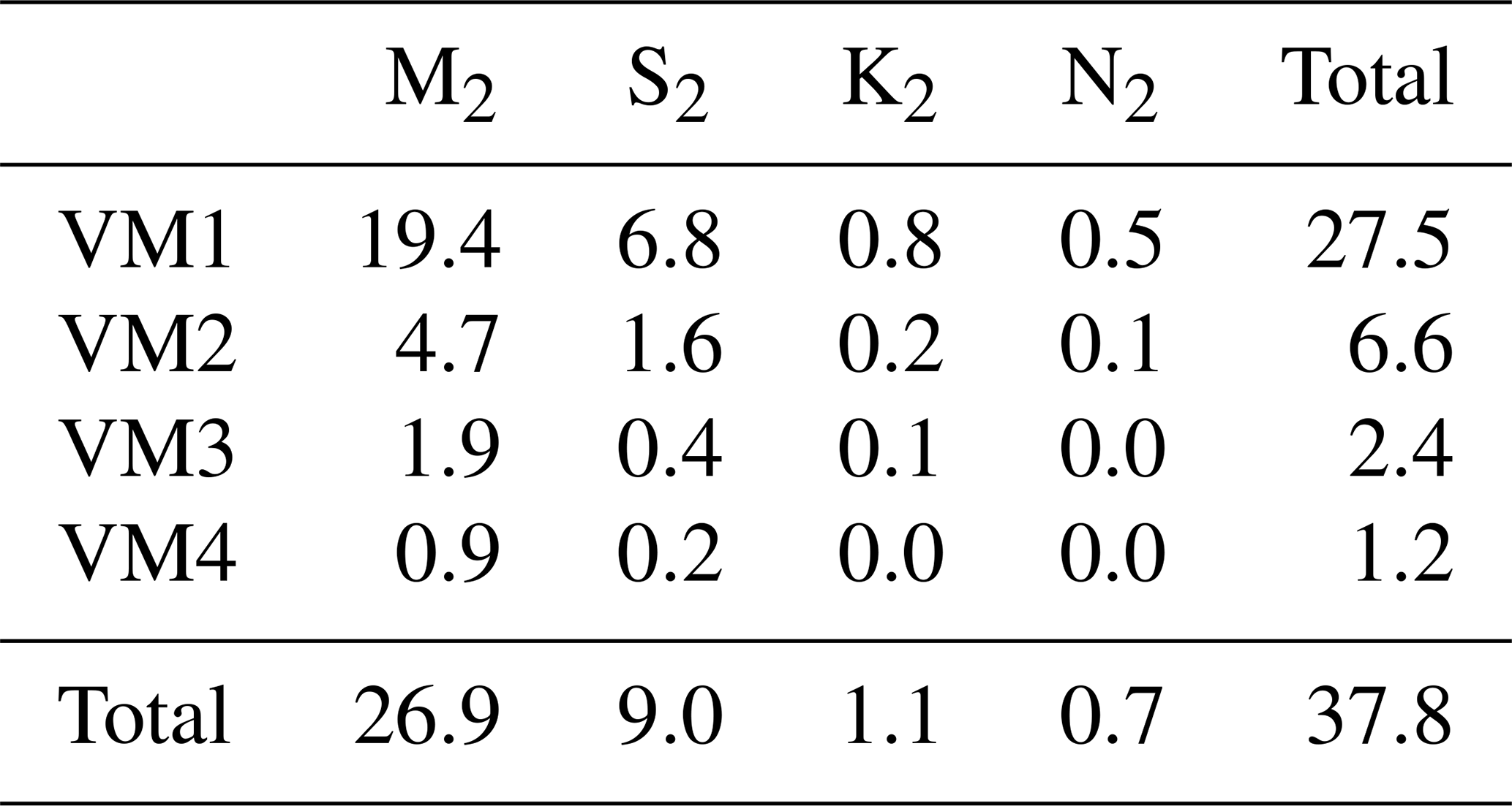
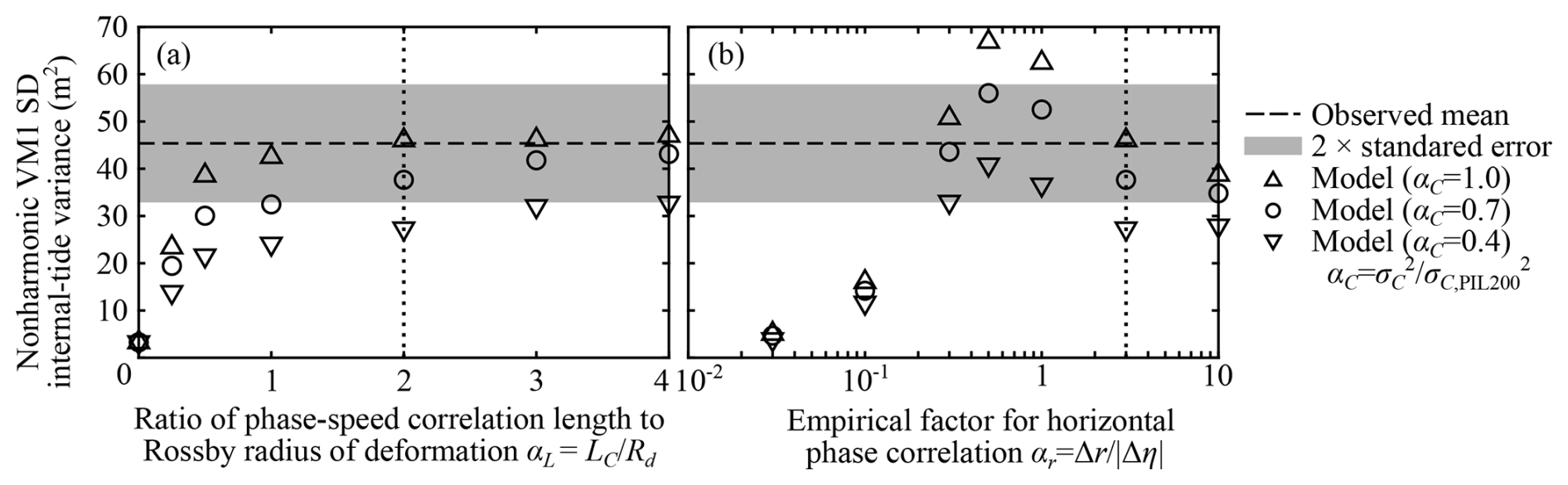
Figure 11 Parameter dependence of the nonharmonic vertical-mode-one (VM1) semidiurnal (SD) internal tide at the PIL200 location. (a) Dependence of internal-tide variance on normalized phase-speed variance α_C and the ratio of phase-speed correlation length to the Rossby radius of deformation α_L, as well as (b) dependence on α_C and the empirical parameter for horizontal correlation of phase modulation α_r. Panels (a) and (b) show results for α_r=3 and α_L=2, respectively. Dotted vertical lines indicate values used in the reference case.

5.6 Dependence on model parameters and comparisons with observations

The results shown in the previous section are based on the reference model parameters, but the parameters have relatively large uncertainty. In this section, we investigate the dependence of the results on the model parameters and compare the results with observations at the PIL200 location. The model parameters are varied beyond the realistic range for process understanding.

The results show that the modelled nonharmonic internal-tide variance strongly depends on the variance (α_C or ${\mathit{\sigma }}_C^{\mathrm{2}}$) and correlation length (α_L or L_C) of phase speed (Fig. 11a). These parameters affect the nonharmonic internal-tide variance in two ways. First, they determine the partitioning of the variance into harmonic and nonharmonic components through the phase variance ${\mathit{\sigma }}_j^{\mathrm{2}}$ (see Eqs. 4b and 4d). Second, they affect the phase correlation length σ_r through μ_j and ς_j in Eq. (7), as well as the variance of horizontal phase difference P_ΔθΔθ in Eqs. (20a)–(20c). The dependence on α_L shows that it is essential to consider the phase-speed correlation length (see the small variance at α_L=0 in Fig. 11a) because phase-speed variability with a small correlation length is inefficient in producing phase variance (see Eq. 19). The dependence on α_L gradually decreases with increasing α_L for a few reasons. First, the ratio of the variance partitioned to nonharmonic component (${\mathit{\varsigma }}_j^{\mathrm{2}}$ in Eq. 4d) increases with the phase variance ${\mathit{\sigma }}_j^{\mathrm{2}}$, but the rate of increase becomes much slower for ${\mathit{\sigma }}_j^{\mathrm{2}}>\mathrm{1}$ (see also Fig. 2d in Part 1 for illustration). Second, the horizontal phase correlation tends to increase nonharmonic internal-tide variance as explained in Appendix C, but the increase ceases when the equivalent isotropic phase correlation length σ_r becomes comparable to the internal-tide wavelength. This is because regions separated by half a wavelength tend to have opposing contributions to internal-tide amplitude (see blue and red patches in Fig. 7), and the opposing contributions are averaged in Eq. (11) when the correlation length is larger than half the wavelength.

The nonharmonic internal-tide variance also strongly depends on α_r (Fig. 11b). The dependence illustrates the aforementioned roles played by the phase correlation length σ_r and internal-tide wavelength more clearly because σ_r is roughly proportional to α_r. The phase correlation increases the nonharmonic internal-tide variance when α_r is small. Although α_r≪1 (negligible horizontal correlation) is unrealistic, small variance in this limit shows that it is essential to consider horizontal phase correlation for gridded sources, as explained in Appendix C. When α_r becomes larger, the nonharmonic internal-tide variance decreases gradually with increasing α_r by the averaging of sources with opposite phases. The peak of the variance should occur when σ_r is around a quarter of the wavelength. Considering that the internal-tide wavelength is 1–2 times the Rossby radius of deformation in the modelled region and σ_r tends to be comparable to but smaller than α_rL_C for VM1, this suggests α_Lα_r is roughly $\mathrm{1}/\mathrm{2}$ at the peak. Figure 11b shows the peak around ${\mathit{\alpha }}_r\approx \mathrm{1}/\mathrm{2}$ for α_L=2. This shows that anisotropy of the horizontal correlation of phase is an important controlling parameter for a realistic parameter range (${\mathit{\alpha }}_L\gtrsim \mathrm{1},{\mathit{\alpha }}_r\gtrsim \mathrm{1}$), especially if α_L≈1. More generally, the result shows that the ratio of the phase correlation length and internal-tide wavelength is important for nonharmonic internal-tide variance.

The comparison of the model results and the PIL200 observations shows that the model results are not inconsistent with the observations for a realistic parameter range (α_L≳1, α_r≳1), although the modelled variance tends to be smaller than the observed mean. The larger phase-speed variance case (α_C=1.0) used phase-speed variance from the PIL200 location on the continental shelf, which provides phase-speed variance that appeared to be roughly the upper limit of previous estimates for deep ocean. In this case, the model results are around the observed mean for α_L≥1. The smaller phase-speed variance case (α_C=0.4) used phase-speed variance that is about the middle of previous estimates for deep ocean but is an underestimate for shallow water. So, it is reasonable that the modelled variance is around or below the approximate 95 % confidence interval for α_L≥1. In the reference case for phase-speed variance (α_C=0.7), the model results are between the observed mean and the lower bound of the approximate 95 % confidence interval for α_L≥1. Considering the number of assumptions and simplifications used in the model suite, the results are encouraging. This demonstrates the feasibility of the proposed modelling framework and model suite.

6 Discussion

This paper developed a new framework and model suite for process-based modelling of nonharmonic internal tides by combining adjoint, statistical, and stochastic approaches. This required the development of a new method called adjoint frequency response analysis and new stochastic models based on stochastic differential equations. (The adjoint frequency response analysis is new in physical oceanography to my knowledge, although the use of the adjoint method in many fields makes a more comprehensive literature survey difficult.) The application of the model suite to nonharmonic vertical-mode-one (VM1) semidiurnal internal tides at the PIL200 location on the Australian North West Shelf added further support that the phase modulation process is caused by phase-speed variability along deterministic (or mean) propagation paths (Zaron and Egbert, 2014) as a first approximation. The correlation length of phase speed and anisotropy of the horizontal correlation of phase modulation were found to be important parameters controlling the nonharmonic internal-tide variance, in addition to phase-speed variance which has been identified in previous studies (Zaron and Egbert, 2014; Buijsman et al., 2017). Furthermore, the nonharmonic variance source function was shown to be a new convenient tool to identify important source regions of nonharmonic internal tides. These are the major novel contributions of this paper.

In the proposed stochastic models, it was aimed to model stochastic wave-phase variables based on the variance and correlation length of phase speed as much as possible. This is because these parameters can be obtained more easily than the phase statistics of nonharmonic internal tides, for example, from reanalysis products that do not include tides. However, since such a study has not been conducted in the modelled region, this study assumed that the phase-speed variance and correlation length were proportional to the observed variance at the PIL200 location and the Rossby radius of deformation, respectively. The use of more realistic phase-speed variance and correlation length would be beneficial for comparing modelled and observed variance in the future.

Since the analysis in Appendix A suggests that nonlinear effects do not have leading-order effects, the most important caveat of the proposed approach appears to be the use of ray tracing and mean stratification to calculate wave propagation paths. The use of ray tracing may be questioned because, when phase-speed variability is included in ray tracing, the length scale of phase-speed variability can be comparable to or shorter than the wavelength (invalidating the slowly varying assumption), and ray paths could vary widely (Park and Watts, 2006; Rainville and Pinkel, 2006). However, studies on wave propagation in random media in other fields (e.g. Ishimaru, 1997; Colosi, 2016) suggest that ray tracing may have wider applicability than it seems. For example, observed phase tends to be insensitive to small-scale phase-speed variability (consistent with Fig. 11a). Even when ray paths diverge widely, the contributions to the observed phase lag may come only from paths around the mean (unperturbed by phase-speed variability) propagation path, called a Fresnel zone. This is because waves arriving through widely perturbed paths tend to have different phases and hence tend to average out through interference. They suggest that phase statistics have relatively weak dependence on the details of ray paths and small-scale phase-speed variability, which appears to be consistent with Buijsman et al. (2017). Ray tracing and mean stratification are used in this study as a compromise among these factors and their simplicity. It would be worth investigating the impact of different methodologies for calculating wave propagation paths in the future.

The proposed model suite aimed to be simple enough to include essential processes only, and this study appears to have achieved the aim; however, the modelled variance tended to be smaller than the observed mean for a realistic range of the model parameters (Fig. 11). The underestimation could have been caused simply by numerical factors (or available computational resources), including insufficient model domain size and grid resolution. It appears likely that at least a few to half a dozen m² of variance were missing for numerical reasons. But the underestimation might also be caused by missing processes of secondary importance, and it would be worth mentioning three potential causes here. First, the amplitude variability of wave sources was neglected. Part 1 showed that the amplitude variability tends to increase nonharmonic internal-tide variance (see Shimizu, 2025, Eq. 14b), although it is less important than the phase variability. Second, the variability of propagation paths was neglected in the model. It might increase phase modulation and make its horizontal correlation more isotropic (effectively larger α_L and smaller α_r), both of which increase nonharmonic internal-tide variance (Fig. 11). Third, Shimizu (2024a) recently showed that the use of the vertical-mode amplitude of surface or isopycnal displacement as an objective function implicitly assumes omnidirectional propagation of internal-wave signals in adjoint models. This implicit assumption might be relevant because the PIL200 observations show that roughly half of the VM1 internal-tide energy is associated with directional waves (but with large uncertainty; see Part 1). Compared to omnidirectional internal tides, internal tides propagating offshore would have higher sensitivity to remote sources in the straits between the Lesser Sunda Islands in Indonesia, although it would have lower sensitivity to remote sources on the Australian shelf.

This study is the first study that took an “inverse” approach to the modelling of nonharmonic internal tides, and the results are promising. Since this is a feasibility study of the new modelling framework, there are many aspects of the model suite that can evolve in the future. For example, the adjoint frequency response analysis assumed linear dynamics, the standard ray theory was used despite potential inadequacies, only phase variability from phase-speed variability along deterministic propagation paths was considered, and the stochastic model for the horizontal phase correlation was highly simplified. Compared to the usual (forward) hydrodynamic modelling, the proposed model suite has complementary characteristics. The model suite focuses on a specific observation location and the statistics of nonharmonic internal tides. It does not yield information for the whole model domain or for a specific time; however, it yields information that is not straightforward to obtain from the usual hydrodynamic modelling, such as the contributions of different source regions (Fig. 10, Table 1) and the dependence on different processes and/or parameters (Fig. 11a and b) for nonharmonic internal tides from distributed sources. For investigating the predictability of nonharmonic internal tides, the locations and quantitative contributions of internal-tide sources, such as in Fig. 10, would provide useful baseline information. It is hoped that the proposed modelling framework provides a useful tool for studying nonharmonic internal tides in the future.

7 Conclusions

Together with Part 1, this study developed a new framework and its implementation for process-based modelling of nonharmonic internal tides by combining adjoint, statistical, and stochastic approaches and applied the resultant model suite to nonharmonic vertical-mode-one (VM1) semidiurnal internal tides at the PIL200 location on the Australian North West Shelf. The proposed modelling framework provides a new tool for process-based studies of nonharmonic internal tides when the superposition of many waves with different degrees of randomness makes process investigation difficult. Also, the combination of adjoint sensitivity modelling and the frequency response analysis from Fourier theory provides a new convenient way to calculate the deterministic sources of internal tides observed at a fixed location. The use of these methods led to the following new findings.

• The modelled nonharmonic internal-tide variance was not inconsistent with the observed variance for a realistic range of the model parameters. This demonstrates the feasibility of the proposed modelling framework and model suite. This also means that, as a first approximation, nonharmonic internal tides are caused by phase-speed variability along the deterministic (or mean) propagation paths.

• Important parameters controlling nonharmonic internal-tide variance include the correlation length of phase speed and anisotropy of the horizontal correlation of phase modulation, in addition to phase-speed variance which has been identified in previous studies.

• A map of the nonharmonic variance source function and its regional integrals provide a new convenient tool to identify important sources of nonharmonic internal tides. For the PIL200 location, important sources include the Australian North West Shelf away from the observation location and the straits between the Lesser Sunda Islands in Indonesia, such as the Lombok Strait.

• Higher vertical modes can be important even when a VM1 internal tide is analysed. In the example application, the highest three of the four lowest baroclinic modes contribute roughly $\mathrm{1}/\mathrm{4}$ of the total variance.

• In addition to the above point, focusing only on VM1 and the M₂ tidal constituent can lead to substantial underestimation of nonharmonic VM1 semidiurnal internal-tide variance, even when they are dominant. In the example application, VM1 and M₂ account for roughly half of the total variance for the four lowest baroclinic modes and the four major semidiurnal constituents.

Appendix A: Nonlinear wave interactions and justification for using linear models

This Appendix provides justification for using a combination of linear models as a first approximation in this study. We do so by deriving the governing equation of approximately linear plane gravity waves affected by nonlinear resonant wave interactions and the variability of background conditions and then considering the order of magnitude of the terms for internal tides. Before the derivation, however, it is worth noting that the cumulative effects of wave modulation caused by strongly nonlinear processes are not necessarily nonlinear in general. This is known in the study field called “wave propagation in random media”. For example, turbulence and short stochastic internal waves (approximately represented by the well-known Garrett–Munk spectrum) are nonlinear, but a signal modulated by these processes can be modelled well by linear methods (e.g. Ishimaru, 1997; Colosi, 2016).

The following derivation has two major differences from many studies of resonant internal-wave interactions in oceanography (see e.g. Müller et al., 1986, for a review). First, we assume modal structure in the vertical instead of vertically propagating internal waves because internal tides are long waves. Second, we consider phase-resolving equations instead of energy or action density equations because we are interested in the phase modulation of internal tides. These approaches were taken in early studies of the resonant wave interactions (e.g. Ball, 1964; Hasselmann, 1966; Thorpe, 1966; see also Olbers and Herterich, 1979, for formulation with the Coriolis effects).

For brevity, the following derivation employs the shallow water equations over a flat bottom under Coriolis effects. This is because the results can be translated to a single baroclinic mode using the vertical-mode formulation in Appendix B in a relatively straightforward manner. The shallow water equations can be written as

$$\begin{array}{}\text{(A1a)}& {\displaystyle }& {\displaystyle \frac{\partial \mathit{\eta }}{\partial t}}=-{\displaystyle \frac{\partial }{\partial x}}\left(\right(h+\mathit{\eta }\left)u\right)-{\displaystyle \frac{\partial }{\partial y}}\left(\right(h+\mathit{\eta }\left)v\right),\text{(A1b)}& {\displaystyle }& {\displaystyle \frac{\partial u}{\partial t}}=-{\displaystyle \frac{\partial }{\partial x}}\left({\displaystyle \frac{c_{\mathrm{0}}^{\mathrm{2}}}{h}}\mathit{\eta }\right)-u{\displaystyle \frac{\partial u}{\partial x}}-v{\displaystyle \frac{\partial u}{\partial y}}+fv,\text{(A1c)}& {\displaystyle }& {\displaystyle \frac{\partial v}{\partial t}}=-{\displaystyle \frac{\partial }{\partial y}}\left({\displaystyle \frac{c_{\mathrm{0}}^{\mathrm{2}}}{h}}\mathit{\eta }\right)-u{\displaystyle \frac{\partial v}{\partial x}}-v{\displaystyle \frac{\partial v}{\partial y}}-fu,\end{array}$$

where h is the constant water depth, $c_{\mathrm{0}}^{\mathrm{2}}=gh$ is the squared celerity, and g is the acceleration due to gravity. Although $c_{\mathrm{0}}^{\mathrm{2}}{h}^{-\mathrm{1}}=g$, the above expression is used for analogy with the evolutionary equations of vertical-mode amplitudes (Eqs. B3a–B3c). We assume that the prognostic variables consist of spatially and temporally varying wave components and spatially uniform random components that are slowly varying in time compared to the wave components (representing mesoscale variability). We also assume that celerity c₀ has a spatially uniform random component (representing, for example, interannual variability of the background conditions), which is assumed to be much smaller than the nonrandom component. Then, we replace the variables in the shallow water equations as

$$\begin{array}{}\text{(A2)}& \left(\begin{array}{c}{c}_{\mathrm{0}}\\ \mathit{\eta }(x,y,t)\\ u(x,y,t)\\ v(x,y,t)\end{array}\right)\to \left(\begin{array}{c}{c}_{\mathrm{0}}\\ \mathrm{0}\\ \mathrm{0}\\ \mathrm{0}\end{array}\right)+\left(\begin{array}{c}{C}_{\mathrm{0}}\\ H\\ U\\ V\end{array}\right)+\left(\begin{array}{c}\mathrm{0}\\ \mathit{\eta }(x,y,t)\\ u(x,y,t)\\ v(x,y,t)\end{array}\right),\end{array}$$

where C₀, H, U, and V are the random components with zero mean (which may result from strongly nonlinear processes), and η, u, and v are the wave components including harmonic and nonharmonic components. Furthermore, we assume that the wave components can be expressed as the superposition of linear plane waves:

$$\begin{array}{}\text{(A3a)}& {\displaystyle }\begin{array}{rl}\mathit{p}& =\sum _j{\mathit{r}}_j{a}_j\left(t\right)e^{-i{\mathit{\theta }}_j^{\prime \prime }\left(t\right)}{e}^{-i\left({\mathit{\kappa }}_{j}x\cos {\mathit{\chi }}_j+{\mathit{\kappa }}_{j}y\sin {\mathit{\chi }}_j-{\mathit{\omega }}_{j}t\right)}\\ & +\left(\mathrm{complex}\mathrm{conjugate}\right),\end{array}\text{(A3b)}& {\displaystyle }\begin{array}{rl}& \mathit{p}=\left[\begin{array}{c}\mathit{\eta }\\ u\\ v\end{array}\right],{\mathit{r}}_j=\left[\begin{array}{c}\mathrm{1}\\ \frac{\mathrm{1}}{{\mathit{\kappa }}_{j}h}\left({\mathit{\omega }}_j\cos {\mathit{\chi }}_j-if\sin {\mathit{\chi }}_j\right)\\ \frac{\mathrm{1}}{{\mathit{\kappa }}_{j}h}\left({\mathit{\omega }}_j\sin {\mathit{\chi }}_j+if\cos {\mathit{\chi }}_j\right)\end{array}\right],\end{array}\end{array}$$

where ${\mathit{\theta }}_j^{\prime \prime }={\mathit{\phi }}_j+{\mathit{\theta }}_j$ is the total phase lag, ω_j is the angular frequency (assumed positive to be consistent with the rest of this study), and κ_j and χ_j are the magnitude and angle of wavenumber vector of the jth wave. Their (real-valued) amplitudes and phases, a_j(t) and ${\mathit{\theta }}_j\left(t\right)={\mathit{\theta }}_j^{\prime \prime }\left(t\right)-\mathit{\phi }\left(t\right)$, correspond to the realization of A_j and Θ_j in Eq. (1). The vectors r_j are right eigenvectors of the linear operator of the shallow water equations:

$$\begin{array}{}\text{(A4)}& \mathbf{L}(\mathit{\kappa },\mathit{\chi })=\left[\begin{array}{ccc}\mathrm{0}& \mathit{\kappa }h\cos \mathit{\chi }& \mathit{\kappa }h\sin \mathit{\chi }\\ \mathit{\kappa }{c}_{\mathrm{0}}^{\mathrm{2}}{h}^{-\mathrm{1}}\cos \mathit{\chi }& \mathrm{0}& -if\\ \mathit{\kappa }{c}_{\mathrm{0}}^{\mathrm{2}}{h}^{-\mathrm{1}}\sin \mathit{\chi }& if& \mathrm{0}\end{array}\right],\end{array}$$

which depends on the wavenumber vector. The right eigenvector r_j satisfies the eigenvalue problem:

$$\begin{array}{}\text{(A5)}& {\displaystyle }{\mathit{\omega }}_j{\mathit{r}}_j=\mathbf{L}\left({\mathit{\kappa }}_j,{\mathit{\chi }}_j\right){\mathit{r}}_j.\end{array}$$

This eigenvalue problem also yields the dispersion relationship ${\mathit{\omega }}_j^{\mathrm{2}}=f^{\mathrm{2}}+c_{\mathrm{0}}^{\mathrm{2}}{\mathit{\kappa }}_j^{\mathrm{2}}$. We substitute Eq. (A3) into Eq. (A1) with Eq. (A2), multiply the equations by $\exp \left(i\right({\mathit{\kappa }}_{j}x\cos {\mathit{\chi }}_j+{\mathit{\kappa }}_{j}y\sin {\mathit{\chi }}_j-{\mathit{\omega }}_{j}t\left)\right)$, and integrate the equations over an area whose size is much larger than the wavelength and over time much longer than the wave period but shorter than the timescale of the random components. The result can be written as

$$\begin{array}{}\text{(A6)}& \begin{array}{rl}{\mathit{r}}_j(i{\mathit{\omega }}_j& +{\displaystyle \frac{\partial }{\partial t}})\left(a_j{e}^{-i{\mathit{\theta }}_j^{\prime \prime }}\right)\\ & =i\left(\mathbf{L}\left({\mathit{\kappa }}_j,{\mathit{\chi }}_j\right)+{\mathit{\kappa }}_j\mathbf{M}\left({\mathit{\chi }}_j\right)\right){\mathit{r}}_j{a}_j{e}^{-i{\mathit{\theta }}_j^{\prime \prime }}\\ & +i\sum _{\mathrm{resonant}k,l}{\mathit{\kappa }}_k\mathbf{N}\left({\mathit{r}}_l,{\mathit{\chi }}_k\right){\mathit{r}}_k{a}_l{a}_k{e}^{-i\left({\mathit{\theta }}_l^{\prime \prime }+{\mathit{\theta }}_k^{\prime \prime }\right)},\end{array}\end{array}$$

where the sum in the last term is taken for combinations that satisfy the resonant triad conditions (Ball, 1964; Hasselmann, 1966; Thorpe, 1966):

$$\begin{array}{}\text{(A7a)}& {\displaystyle }& {\displaystyle }{\mathit{\omega }}_j\pm {\mathit{\omega }}_k\pm {\mathit{\omega }}_l=\mathrm{0},\text{(A7b)}& {\displaystyle }& {\displaystyle }{\overrightarrow{\mathit{\kappa }}}_j\pm {\overrightarrow{\mathit{\kappa }}}_k\pm {\overrightarrow{\mathit{\kappa }}}_l=\overrightarrow{\mathrm{0}},\end{array}$$

and $\overrightarrow{\mathit{\kappa }}=\mathit{\kappa }(\cos \mathit{\chi },\sin \mathit{\chi })$ is the wavenumber vector. The matrix operators are defined as

$$\begin{array}{}\text{(A8a)}& {\displaystyle }\begin{array}{rl}& \mathbf{M}\left(\mathit{\chi }\right)=\\ & \left[\begin{array}{ccc}U\cos \mathit{\chi }+V\sin \mathit{\chi }& H\cos \mathit{\chi }& H\sin \mathit{\chi }\\ \mathrm{2}{c}_{\mathrm{0}}{C}_{\mathrm{0}}{h}^{-\mathrm{1}}\cos \mathit{\chi }& U\cos \mathit{\chi }+V\sin \mathit{\chi }& \mathrm{0}\\ \mathrm{2}{c}_{\mathrm{0}}{C}_{\mathrm{0}}{h}^{-\mathrm{1}}\sin \mathit{\chi }& \mathrm{0}& U\cos \mathit{\chi }+V\sin \mathit{\chi }\end{array}\right],\end{array}\text{(A8b)}& {\displaystyle }\begin{array}{rl}& \mathbf{N}(\mathit{p},\mathit{\chi })=\\ & \left[\begin{array}{ccc}u\cos \mathit{\chi }+v\sin \mathit{\chi }& \mathit{\eta }\cos \mathit{\chi }& \mathit{\eta }\sin \mathit{\chi }\\ \mathrm{0}& u\cos \mathit{\chi }+v\sin \mathit{\chi }& \mathrm{0}\\ \mathrm{0}& \mathrm{0}& u\cos \mathit{\chi }+v\sin \mathit{\chi }\end{array}\right],\end{array}\end{array}$$

where the argument p of N corresponds to (η, u, v) in the matrix, and $\left|C_{\mathrm{0}}\right|\ll c_{\mathrm{0}}$ is assumed in M. It is convenient to reduce Eq. (A6) to a scalar differential equation. This can be done by using the left eigenvectors of L:

$$\begin{array}{}\text{(A9)}& {\mathit{l}}_j=\left[\begin{array}{c}\frac{c_{\mathrm{0}}^{\mathrm{2}}}{h}\\ \frac{\mathrm{1}}{{\mathit{\kappa }}_j}\left({\mathit{\omega }}_j\cos {\mathit{\chi }}_j-if\sin {\mathit{\chi }}_j\right)\\ \frac{\mathrm{1}}{{\mathit{\kappa }}_j}\left({\mathit{\omega }}_j\sin {\mathit{\chi }}_j+if\cos {\mathit{\chi }}_j\right)\end{array}\right],\end{array}$$

which forms a pair with r_j. By left-multiplying Eq. (A6) by ${\mathit{l}}_j^H$, we get

$$\begin{array}{}\text{(A10)}& \left(i{\mathit{\omega }}_j+{\displaystyle \frac{\partial }{\partial t}}\right)\left(a_j{e}^{-i{\mathit{\theta }}_j^{\prime \prime }}\right)=i{\mathit{\omega }}_j\left(\mathrm{1}+{\displaystyle \frac{c^{\prime }}{\stackrel{\mathrm{‾}}{c}}}+n_j\right)\left(a_j{e}^{-i{\mathit{\theta }}_j^{\prime \prime }}\right),\end{array}$$

where $c={\mathit{\omega }}_j/{\mathit{\kappa }}_j$ is the phase speed of the “carrier” wave (the exponential function in Eq. A3), $\stackrel{\mathrm{‾}}{c}$ is the (mean) phase speed in the absence of the random components (C₀, H, U, V), c^′ is the phase-speed deviation due to modulation by the random components, and n_j is defined shortly. The first term on the right-hand side is obtained using Eq. (A5). The second term is obtained using

$$\begin{array}{}\text{(A11)}& \begin{array}{rl}{\mathit{\kappa }}_j& {\displaystyle \frac{{\mathit{l}}_j^H\mathbf{M}\left({\mathit{\chi }}_j\right){\mathit{r}}_j}{{\mathit{l}}_j^H{\mathit{r}}_j}}\\ & =\left({\displaystyle \frac{c_{\mathrm{0}}{C}_{\mathrm{0}}}{{\stackrel{\mathrm{‾}}{c}}^{\mathrm{2}}}}+{\displaystyle \frac{U\cos \mathit{\chi }+V\sin \mathit{\chi }}{\stackrel{\mathrm{‾}}{c}}}+{\displaystyle \frac{c_{\mathrm{0}}^{\mathrm{2}}}{\mathrm{2}{\stackrel{\mathrm{‾}}{c}}^{\mathrm{2}}}}{\displaystyle \frac{H}{h}}\right){\mathit{\omega }}_j\\ & ={\displaystyle \frac{c^{\prime }}{\stackrel{\mathrm{‾}}{c}}}{\mathit{\omega }}_j.\end{array}\end{array}$$

The fact that c^′ is the phase-speed deviation can be checked by deriving the dispersion relationship including the random components. The first two terms of c^′ agree with Zaron and Egbert (2014) (except for an error regarding $c_p^{\mathrm{2}}$ and gD in the denominator in their Eq. A12). The third term is the resonant wave interaction term, where $n_j(a_j,a_k,a_l,{\mathit{\theta }}_j^{\prime \prime },{\mathit{\theta }}_k^{\prime \prime },{\mathit{\theta }}_l^{\prime \prime },{\mathit{\chi }}_j,{\mathit{\chi }}_k,{\mathit{\chi }}_l)$ is defined as

$$\begin{array}{}\text{(A12a)}& {\displaystyle }\begin{array}{rl}{n}_j& ={\displaystyle \frac{e^{i{\mathit{\theta }}_j^{\prime \prime }}}{a_j{\mathit{\omega }}_j}}\sum _{\mathrm{resonant}k,l}{\mathit{\kappa }}_k{\displaystyle \frac{{\mathit{l}}_j^H\mathbf{N}\left({\mathit{r}}_l,{\mathit{\chi }}_k\right){\mathit{r}}_k}{{\mathit{l}}_j^H{\mathit{r}}_j}}{a}_l{a}_k{e}^{-i\left({\mathit{\theta }}_l^{\prime \prime }+{\mathit{\theta }}_k^{\prime \prime }\right)}\\ & ={\displaystyle \frac{c_{\mathrm{0}}^{\mathrm{2}}}{\mathrm{2}{\stackrel{\mathrm{‾}}{c}}^{\mathrm{2}}}}\sum _{\mathrm{resonant}k,l}\left(\mathrm{1}+{\displaystyle \frac{{\mathit{\kappa }}_k}{{\mathit{\kappa }}_l}}{f}_{\mathrm{1}}{f}_{\mathrm{2}}\right){\displaystyle \frac{{\mathit{\omega }}_k}{{\mathit{\omega }}_j}}{\displaystyle \frac{a_l{a}_k}{a_{j}h}}{e}^{-i\left({\mathit{\theta }}_l^{\prime \prime }+{\mathit{\theta }}_k^{\prime \prime }-{\mathit{\theta }}_j^{\prime \prime }\right)},\end{array}\text{(A12b)}& {\displaystyle }\begin{array}{rl}& f_{\mathrm{1}}=\mathrm{1}+\\ & {\displaystyle \frac{\left({\mathit{\omega }}_j{\mathit{\omega }}_k+f^{\mathrm{2}}\right)\cos \left({\mathit{\chi }}_j-{\mathit{\chi }}_k\right)+if\left({\mathit{\omega }}_j+{\mathit{\omega }}_k\right)\sin \left({\mathit{\chi }}_j-{\mathit{\chi }}_k\right)}{c_{\mathrm{0}}^{\mathrm{2}}{\mathit{\kappa }}_j{\mathit{\kappa }}_k}},\end{array}\text{(A12c)}& {\displaystyle }\begin{array}{rl}& f_{\mathrm{2}}={\displaystyle \frac{{\mathit{\omega }}_l}{{\mathit{\omega }}_k}}\cos \left({\mathit{\chi }}_l-{\mathit{\chi }}_k\right)-i{\displaystyle \frac{f}{{\mathit{\omega }}_k}}\sin \left({\mathit{\chi }}_l-{\mathit{\chi }}_k\right).\end{array}\end{array}$$

The first terms on both sides of Eq. (A10) obviously cancel each other, but they are retained to show the magnitude of the unmodulated linear solution. Finally, by separating the real and imaginary parts of Eq. (A10) and recalling ${\mathit{\theta }}_j^{\prime \prime }={\mathit{\phi }}_j+{\mathit{\theta }}_j$, we get the evolutionary equations of wave amplitudes and phases:

$$\begin{array}{}\text{(A13a)}& {\displaystyle }& {\displaystyle \frac{\partial a_j}{\partial t}}=-a_j{\mathit{\omega }}_{j}Im\left(n_j\right),\text{(A13b)}& {\displaystyle }& {\displaystyle \frac{\partial \left({\mathit{\phi }}_j+{\mathit{\theta }}_j\right)}{\partial t}}=-{\mathit{\omega }}_j\left({\displaystyle \frac{c^{\prime }}{\stackrel{\mathrm{‾}}{c}}}+Re\left(n_j\right)\right).\end{array}$$

The above analysis can be applied to internal tides using the vertical-mode formulation in Appendix B. To simplify the argument, we consider only vertical mode one (VM1), although inter-mode interactions are required to satisfy the resonant triad conditions in Eq. (A7) in general (Hasselmann, 1966). This is because (i) nonlinear wave excitation can also occur at near-resonant conditions, (ii) the inclusion of vertical mode two (VM2) does not change the following order-of-magnitude argument for the PIL200 location, and (iii) it appears that there is no previous study that investigated nonharmonic internal-tide variance for higher modes in the deep water within the model domain. To consider VM1, we replace c₀ and h by the celerity and normalization factor of VM1, c₁ and ${\widehat{h}}_{\mathrm{1}}$, and the prognostic variables (η, u, v) by the corresponding VM1 amplitudes (${\widehat{\mathit{\eta }}}_{\mathrm{1}}$, ${\widehat{u}}_{\mathrm{1}}$, ${\widehat{v}}_{\mathrm{1}}$). We also make the corresponding changes to the random components (C₀, H, U, V) and multiply the matrix N by the nonlinear interaction coefficient ${\widehat{N}}_{\mathrm{111}}$ defined in Eq. (B4c).

We now consider the order of magnitude of the unmodulated linear (first), modulated linear (second), and nonlinear (third) terms on the right-hand side of Eq. (A10) for VM1 semidiurnal internal tides. The ratio of the modulated term to the unmodulated term is $c^{\prime }/\stackrel{\mathrm{‾}}{c}$, which is about 0.1 at the PIL200 location on the Australian North West Shelf (approximately 200 m water depth) and 0.01 to 0.03 in deep ocean (see Appendix F and Sect, 4.3). For the nonlinear excitation of semidiurnal internal tides, the major nonlinear contributions come from diurnal–diurnal interactions (e.g. ${\mathit{\omega }}_{{\mathrm{K}}_{\mathrm{2}}}={\mathit{\omega }}_{{\mathrm{K}}_{\mathrm{1}}}+{\mathit{\omega }}_{{\mathrm{K}}_{\mathrm{1}}}$) and semidiurnal–quarter-diurnal interactions (e.g. ${\mathit{\omega }}_{{\mathrm{M}}_{\mathrm{2}}}={\mathit{\omega }}_{{\mathrm{M}}_{\mathrm{4}}}-{\mathit{\omega }}_{{\mathrm{M}}_{\mathrm{2}}}$). (Note that the effects of low-frequency variability are included in c^′.) Neglecting O(1) factors $c_{\mathrm{0}}^{\mathrm{2}}/{\stackrel{\mathrm{‾}}{c}}^{\mathrm{2}}$ and ${\mathit{\omega }}_k/{\mathit{\omega }}_j$ in Eq. (A12), the ratio of the nonlinear term to the unmodulated linear term is $O\left(\right|{\widehat{N}}_{\mathrm{111}}|a_l{a}_k/({\widehat{h}}_{\mathrm{1}}{a}_j\left)\right)$. For diurnal–diurnal and semidiurnal–quarter-diurnal interactions, the ratios are about 0.002 and 0.01 at the PIL200 location, respectively. (These values are obtained using ${\widehat{h}}_{\mathrm{1}}=\mathrm{40}$ m, ${\widehat{N}}_{\mathrm{111}}=\mathrm{0.17}$, a_D=1.5 m, a_SD=6.4 m, and a_QD=2.2 m for VM1 from Part 1, where a_D, a_SD, and a_QD are the VM1 internal-tide amplitudes corresponding to half the harmonic plus nonharmonic variance over diurnal, semidiurnal, and quarter-diurnal frequency bands, respectively.) For the deep ocean within the model domain, VM1 semidiurnal (harmonic plus nonharmonic) internal-tide amplitudes appear to have the same order of magnitude as the PIL200 location (e.g. compare the surface displacement variance of 0.6 cm², from Table 2 in Part 1, with the “F-space” approach by Nelson et al., 2019). On the abyssal plain between the Australian North West Shelf and Indonesia (i.e. Argo Abyssal Plain), for example, we get ${\widehat{h}}_{\mathrm{1}}\approx \mathrm{700}$ m, ${\widehat{N}}_{\mathrm{111}}\approx -\mathrm{0.9}$, and $\left|{\widehat{N}}_{\mathrm{111}}\right|a_l{a}_k/\left({\widehat{h}}_{\mathrm{1}}{a}_j\right)=\mathrm{0.0005}$ by normalizing the vertical mode for isopycnal displacement by the maximum value and by using a_D and a_SD from the PIL200 location and the climatological stratification used in the adjoint modelling (Sect. 4.2). These values suggest that the nonlinear term is an order of magnitude smaller than the modulation term both in the deep ocean and on the Australian continental shelf, probably excluding shallower parts of the shelf (say, approximately or less than 100 m water depth). Note that the random components are assumed to be spatially uniform for brevity in the above analysis; however, the contributions of background currents and background vorticity to c^′ (Zaron and Egbert, 2014, Eq. A12) suggest that the assumption does not change the order of magnitude of the terms provided that the horizontal scale of the random variability is comparable to or larger than the Rossby radius of deformation.

The above analysis suggests that the nonlinear resonant wave interactions during wave propagation can be neglected as a first approximation for VM1 semidiurnal internal tides. Then, recalling that φ_j represents the expected (harmonic) phase lags defined in the absence of c^′, the mean of Eq. (A13) shows that the pre-modulation amplitudes a_j and phase lags φ_j remain approximately constant. So, they can be evaluated at the sources, as done in the adjoint frequency response analysis. Also, by subtracting the mean from Eq. (A13b), we get the evolutionary equations of θ_j(t), equivalent to Eq. (16), which is the basis of the proposed linear stochastic phase modelling. They provide justification for using a combination of linear models as a first approximation in this study. Also, Eq. (A13b) provides another justification for calculating phase deviation from phase-speed deviation, as suggested by Zaron and Egbert (2014).

Appendix B: Governing equations of vertical-mode amplitudes and formulation of hydrodynamic model

This Appendix describes the evolutionary equations of vertical-mode amplitudes over steep slopes, which are used for three purposes in this paper: (i) the numerical hydrodynamic model used for adjoint sensitivity modelling (Sect. 4.2), (ii) scaling of the modulation and nonlinear terms to justify linear modelling (Appendix A), and (iii) the estimation of phase-speed variance from the PIL200 observations (Appendix F). The approach was originally proposed by Griffiths and Grimshaw (2007) to my knowledge and formulated in a more convenient form and extended to include full nonlinear and nonhydrostatic effects by Shimizu (2011, 2017, 2019). The linear formulation by Shimizu (2011) was adopted, for example, by Zaron and Egbert (2014) and Kelly et al. (2016). These studies used horizontally variable vertical modes, which are calculated using local water depth and background stratification. For example, using the generalized isopycnal coordinate s that depends only on density ρ and explicitly writing the horizontal vector components (unlike the main body of this paper, $\overrightarrow{x}=(x,y)$) for clarity, the isopycnal displacement η and the horizontal velocity (u, v) can be decomposed as (Shimizu, 2019)

$$\begin{array}{}\text{(B1a)}& {\displaystyle }& {\displaystyle }\mathit{\eta }(x,y,s,t)=\sum _n{\widehat{\mathit{\varphi }}}_n(x,y,s){\widehat{\mathit{\eta }}}_n(x,y,t),\text{(B1b)}& {\displaystyle }& {\displaystyle }u(x,y,s,t)=\sum _n{\widehat{\mathit{\pi }}}_n(x,y,s){\widehat{u}}_n(x,y,t),\text{(B1c)}& {\displaystyle }& {\displaystyle }v(x,y,s,t)=\sum _n{\widehat{\mathit{\pi }}}_n(x,y,s){\widehat{v}}_n(x,y,t),\end{array}$$

where the sum is taken over all available vertical modes, ${\widehat{\mathit{\eta }}}_n$, ${\widehat{u}}_n$, and ${\widehat{v}}_n$ are the nth vertical-mode amplitudes of the corresponding prognostic variable, and ${\widehat{\mathit{\varphi }}}_n$ and ${\widehat{\mathit{\pi }}}_n$ are the nth vertical modes for isopycnal displacement and horizontal velocity, respectively. In this paper, the subscripts m and n denote vertical mode indices, which are 0 for the barotropic mode, 1 for the first baroclinic mode, and so on. Each set of vertical modes (${\widehat{\mathit{\varphi }}}_n$, ${\widehat{\mathit{\pi }}}_n$) has the associated celerity (or the propagation speed of non-rotating linear long gravity waves) c_n and normalization factor ${\widehat{h}}_n$ with the unit of water depth. The normalization factor is defined as

$$\begin{array}{}\text{(B2a)}& \widehat{\mathit{\rho }}{\widehat{h}}_n=\underset{s^b}{\overset{s^t}{\int }}{\widehat{\mathit{\pi }}}_n\mathit{\rho }{\displaystyle \frac{\mathrm{d}Z}{\mathrm{d}s}}{\widehat{\mathit{\pi }}}_n\mathrm{d}s,\end{array}$$

where $\widehat{\mathit{\rho }}$ is a reference density, and $Z(x,y,s)$ is the background height of isopycnal. Hereafter, the superscripts t and b denote the values at the surface and bottom, respectively. Since the choices of $\widehat{\mathit{\rho }}$ and ${\widehat{h}}_n$ are arbitrary, a hat is used to denote variables whose magnitudes depend on these normalization factors.

For approximately linear hydrostatic problems considered in this study, the multi-layer formulation in Shimizu (2011) and the continuous formulation in Shimizu (2019) become equivalent after vertical-mode decomposition. We assume c_n≪c₀ for n>0 and retain the nonlinear terms for scaling purposes (but neglect mixed nonlinear–topographic terms). Then, separating known barotropic (tidal) currents as external forcing and neglecting other forcing and dissipation processes except linear bottom friction, the governing equations for ${\widehat{\mathit{\eta }}}_n$, ${\widehat{u}}_n$, and ${\widehat{v}}_n$ for n>0 are approximately given by

$$\begin{array}{}\text{(B3a)}& {\displaystyle }\begin{array}{rl}{\displaystyle \frac{\partial {\widehat{\mathit{\eta }}}_n}{\partial t}}& =-{\displaystyle \frac{\partial }{\partial x}}\left({\widehat{h}}_n{\widehat{u}}_n\right)-\sum _{l,m>\mathrm{0}}{\displaystyle \frac{\partial }{\partial x}}\left({\widehat{N}}_{mln}{\widehat{\mathit{\eta }}}_l{\widehat{u}}_m\right)\\ & -{\displaystyle \frac{\partial }{\partial y}}\left({\widehat{h}}_n{\widehat{v}}_n\right)-\sum _{l,m>\mathrm{0}}{\displaystyle \frac{\partial }{\partial y}}\left({\widehat{N}}_{mln}{\widehat{\mathit{\eta }}}_l{\widehat{v}}_m\right)\\ & +\sum _{m>\mathrm{0}}\left({\widehat{L}}_{mn}^x{\widehat{h}}_m{\widehat{u}}_m+{\widehat{L}}_{mn}^y{\widehat{h}}_m{\widehat{v}}_m\right)+{\widehat{f}}_n^{\mathit{\eta }},\end{array}\text{(B3b)}& {\displaystyle }\begin{array}{rl}{\displaystyle \frac{\partial {\widehat{u}}_n}{\partial t}}& =-{\displaystyle \frac{\partial }{\partial x}}\left({\displaystyle \frac{c_n^{\mathrm{2}}}{{\widehat{h}}_n}}{\widehat{\mathit{\eta }}}_n\right)-\sum _{l,m>\mathrm{0}}{\widehat{N}}_{lnm}\left({\widehat{u}}_l{\displaystyle \frac{\partial {\widehat{u}}_m}{\partial x}}+{\widehat{v}}_l{\displaystyle \frac{\partial {\widehat{u}}_m}{\partial y}}\right)\\ & -\sum _{m>\mathrm{0}}{\widehat{L}}_{nm}^x{\displaystyle \frac{c_m^{\mathrm{2}}}{{\widehat{h}}_m}}{\widehat{\mathit{\eta }}}_m+f{\widehat{v}}_n-{\displaystyle \frac{\mathrm{1}}{{\widehat{h}}_n}}\sum _{m>\mathrm{0}}{\widehat{\mathrm{\Gamma }}}_{nm}{\widehat{u}}_m,\end{array}\text{(B3c)}& {\displaystyle }\begin{array}{rl}{\displaystyle \frac{\partial {\widehat{v}}_n}{\partial t}}& =-{\displaystyle \frac{\partial }{\partial y}}\left({\displaystyle \frac{c_n^{\mathrm{2}}}{{\widehat{h}}_n}}{\widehat{\mathit{\eta }}}_n\right)-\sum _{l,m>\mathrm{0}}{\widehat{N}}_{lnm}\left({\widehat{u}}_l{\displaystyle \frac{\partial {\widehat{v}}_m}{\partial x}}+{\widehat{v}}_l{\displaystyle \frac{\partial {\widehat{v}}_m}{\partial y}}\right)\\ & -\sum _{m>\mathrm{0}}{\widehat{L}}_{nm}^y{\displaystyle \frac{c_m^{\mathrm{2}}}{{\widehat{h}}_m}}{\widehat{\mathit{\eta }}}_m-f{\widehat{u}}_n-{\displaystyle \frac{\mathrm{1}}{{\widehat{h}}_n}}\sum _{m>\mathrm{0}}{\widehat{\mathrm{\Gamma }}}_{nm}{\widehat{v}}_m.\end{array}\end{array}$$

Here, ${\widehat{f}}_n^{\mathit{\eta }}$ represents the forcing function from the barotropic to nth baroclinic mode (shown in Fig. 3 for VM1 M₂ tide), ${\widehat{L}}_{nm}^x$ and ${\widehat{L}}_{nm}^y$ are topographic interaction coefficients, ${\widehat{N}}_{nlm}$ represents nonlinear interaction coefficients, and ${\widehat{\mathrm{\Gamma }}}_{nm}$ represents modal friction coefficients. These variables are defined as

$$\begin{array}{}\text{(B4a)}& {\displaystyle }& {\displaystyle }{\widehat{f}}_n^{\mathit{\eta }}={\widehat{L}}_{\mathrm{0}n}^x{\widehat{h}}_{\mathrm{0}}{\widehat{u}}_{\mathrm{0}}+{\widehat{L}}_{\mathrm{0}n}^y{\widehat{h}}_{\mathrm{0}}{\widehat{v}}_{\mathrm{0}},\text{(B4b)}& {\displaystyle }& {\displaystyle }{\widehat{L}}_{nm}^x={\displaystyle \frac{\mathrm{1}}{\widehat{\mathit{\rho }}{\widehat{h}}_n}}\underset{s^b}{\overset{s^t}{\int }}{\widehat{\mathit{\pi }}}_n\mathit{\rho }{\displaystyle \frac{\mathrm{d}Z}{\mathrm{d}s}}{\displaystyle \frac{\partial {\widehat{\mathit{\pi }}}_m}{\partial x}}\mathrm{d}s,\text{(B4c)}& {\displaystyle }& {\displaystyle }{\widehat{N}}_{nlm}={\displaystyle \frac{\mathrm{1}}{\widehat{\mathit{\rho }}{\widehat{h}}_l}}\underset{s^b}{\overset{s^t}{\int }}{\widehat{\mathit{\pi }}}_n\mathit{\rho }{\displaystyle \frac{\mathrm{d}Z}{\mathrm{d}s}}{\widehat{\mathit{\pi }}}_l{\widehat{\mathit{\pi }}}_m\mathrm{d}s,\text{(B4d)}& {\displaystyle }& {\displaystyle }{\widehat{\mathrm{\Gamma }}}_{nm}={\displaystyle \frac{\mathit{\gamma }}{\widehat{\mathit{\rho }}}}{\widehat{\mathit{\pi }}}_n^b{\mathit{\rho }}^b{\widehat{\mathit{\pi }}}_m^b,\end{array}$$

where γ is the linear friction coefficient. The variable ${\widehat{L}}_{nm}^y$ is defined similarly by replacing x by y in Eq. (B4b).

For numerical hydrodynamic modelling, Eqs. (B3a)–(B3c) excluding the nonlinear terms (i.e. those with ${\widehat{N}}_{nlm}$) are discretized using the control volume (or finite-volume) method on the staggered (or Arakawa-C) grid, assuming a sinusoidal motion with angular frequency ω. Then, the matrix operator is set up for the model state vector ${\left[\begin{array}{cccccc}{\widehat{\mathit{\eta }}}_{\mathrm{1}}{\widehat{\mathit{\eta }}}_{\mathrm{2}}& \mathrm{\cdots }& {\widehat{u}}_{\mathrm{1}}{\widehat{u}}_{\mathrm{2}}& \mathrm{\cdots }& {\widehat{v}}_{\mathrm{1}}{\widehat{v}}_{\mathrm{2}}& \mathrm{\cdots }\end{array}\right]}^T$, and the matrix operator is transposed to obtain the operator for the adjoint model, L^H in Eq. (D7).

Appendix C: Detailed points regarding the treatment of horizontal correlation using ${\mathbf{R}}^{\mathrm{1}/\mathrm{2}}$

This Appendix describes three detailed points regarding the treatment of horizontal correlation using ${\mathbf{R}}^{\mathrm{1}/\mathrm{2}}$ in Eqs. (11) and (12) in Sect. 3.1.

The first point is that ${\mathbf{R}}^{\mathrm{1}/\mathrm{2}}$ is not unique for the same R. For example, if sources at two locations are perfectly correlated with s_phys=[s₀ s₀]^T and Σ=ς₀I, R is a matrix with all the elements being unity. The Cholesky decomposition, a common numerical method to calculate ${\mathbf{R}}^{\mathrm{1}/\mathrm{2}}$, yields

$$\begin{array}{}\text{(C1)}& {\mathbf{R}}^{\mathrm{1}/\mathrm{2}}=\left[\begin{array}{cc}\mathrm{1}& \mathrm{0}\\ \mathrm{1}& \mathrm{0}\end{array}\right].\end{array}$$

Then, s_stat=[2s₀ 0]^T from Eq. (11). This is reasonable in that statistically independent sources consist of a single source whose complex-valued amplitude is the sum of those of two perfectly correlated sources. But it also has a problem that the ordering of vector elements in s_phys determines where this single source is located. An alternative choice of ${\mathbf{R}}^{\mathrm{1}/\mathrm{2}}$ is

$$\begin{array}{}\text{(C2)}& {\mathbf{R}}^{\mathrm{1}/\mathrm{2}}={\displaystyle \frac{\mathrm{1}}{\sqrt{\mathrm{2}}}}\left[\begin{array}{cc}\mathrm{1}& \mathrm{1}\\ \mathrm{1}& \mathrm{1}\end{array}\right].\end{array}$$

In this case, ${\mathit{s}}_{\mathrm{stat}}=[\sqrt{\mathrm{2}}{s}_{\mathrm{0}}\sqrt{\mathrm{2}}{s}_{\mathrm{0}}{]}^T$. It is not intuitive to have two supposedly independent sources for two perfectly correlated sources. However, it has an advantage that the result does not depend on the ordering of vector elements in s_phys, and there is a numerical method to calculate this type of ${\mathbf{R}}^{\mathrm{1}/\mathrm{2}}$ much more efficiently (the diffusion operator method by Weaver and Courtier, 2001) than the Cholesky decomposition for large problems. Importantly, in both cases, $E\left({A^{\prime }}^{\mathrm{2}}\right)=\mathrm{4}|s_{\mathrm{0}}{|}^{\mathrm{2}}{\mathit{\varsigma }}_{\mathrm{0}}^{\mathrm{2}}$ from Eq. (12) because $\mathbf{R}={\mathbf{R}}^{\mathrm{1}/\mathrm{2}}{\mathbf{R}}^{T/\mathrm{2}}$ is the same. These examples suggest that s_stat provides effectively independent sources that can be used in the statistical model to calculate nonharmonic internal-tide variance, but the horizontal distribution of the independent sources is uncertain within the correlation length of phase modulation.

The second point is that the horizontal phase correlation has a large impact on nonharmonic internal-tide variance. As a simple example, consider the above two-source case but in the absence of horizontal correlation. Then, ${\mathbf{R}}^{\mathrm{1}/\mathrm{2}}=\mathbf{I}$ and $E\left({A^{\prime }}^{\mathrm{2}}\right)=\mathrm{2}|s_{\mathrm{0}}{|}^{\mathrm{2}}{\mathit{\varsigma }}_{\mathrm{0}}^{\mathrm{2}}$ from Eq. (12), which is half of the above perfectly correlated cases. It is important to relate this to grid resolution in a numerical hydrodynamic model. If one source region is resolved by one grid point with s_phys=[2s₀] and Σ=ς₀ in a low-resolution model and two grid points with s_phys=[s₀ s₀]^T and Σ=ς₀I in the corresponding high-resolution model, the sum of s_phys (i.e. pre-modulation internal-tide amplitude) is the same (i.e. 2s₀). However, if we neglect the horizontal correlation of the sources, the variance is $E\left({A^{\prime }}^{\mathrm{2}}\right)=\mathrm{4}|s_{\mathrm{0}}{|}^{\mathrm{2}}{\mathit{\varsigma }}_{\mathrm{0}}^{\mathrm{2}}$ in the low-resolution case and $\mathrm{2}|s_{\mathrm{0}}{|}^{\mathrm{2}}{\mathit{\varsigma }}_{\mathrm{0}}^{\mathrm{2}}$ in the high-resolution case. The perfect correlation considered in the last paragraph is required to make the variance the same at the two resolutions. This shows that the horizontal correlation has to be considered for gridded sources; otherwise, the results would be highly dependent on grid resolution.

The third point is that, strictly speaking, the treatment of horizontal correlation using ${\mathbf{R}}^{\mathrm{1}/\mathrm{2}}$ cannot be used to investigate the details of the PDF or higher moments because the statistical model uses a non-Gaussian distribution on the complex plane for individual wave components. However, the method based on ${\mathbf{R}}^{\mathrm{1}/\mathrm{2}}$ works in the limit of many independent sources (or when the central limit theorem is applicable) because the limiting distribution is determined by the (co)variance, regardless of the PDF of individual sources. The results of Part 1 suggest that this “many source” limit is common for internal tides.

Appendix D: Adjoint method and adjoint frequency response analysis

This Appendix describes the adjoint method and adjoint frequency response analysis used to solve the covariance equations and to calculate the source function. We start from a quick overview of the adjoint method, which is often used in so-called four-dimensional variational data assimilation in physical oceanography (e.g. Bennett, 2002; Wunsch, 2006).

The adjoint method is based on a so-called forward model and an objective (or cost) function. We consider a linear model,

$$\begin{array}{}\text{(D1)}& {\displaystyle \frac{\partial \mathit{x}}{\partial t}}=-\mathbf{L}\mathit{x}+\mathit{f},\end{array}$$

where x(t) is the model state vector containing the model's prognostic variables, L is the matrix operator representing the linear dynamics, and f is the external forcing. Since the model is linear, the solution can be written as

$$\begin{array}{}\text{(D2)}& \mathit{x}\left(t\right)=\underset{-\mathrm{\infty }}{\overset{t}{\int }}\mathbf{H}(t-\mathit{\tau })\mathit{f}\left(\mathit{\tau }\right)\mathrm{d}\mathit{\tau },\end{array}$$

where each column of the matrix H contains the impulse response function. Using the model solution, we consider a linear function J=w^Hx, tentatively defined at a particular time t_j. The variable w is the time-independent weight vector used to define J. There are various expressions for J:

$$\begin{array}{}\text{(D3a)}& {\displaystyle }J\left(t_j\right)& {\displaystyle }={\mathit{w}}^H\mathit{x}\left(t_j\right)\text{(D3b)}& {\displaystyle }& {\displaystyle }=\underset{-\mathrm{\infty }}{\overset{t_j}{\int }}{\left({\mathbf{H}}^H\left(t_j-\mathit{\tau }\right)\mathit{w}\right)}^H\mathit{f}\left(\mathit{\tau }\right)\mathrm{d}\mathit{\tau }\text{(D3c)}& {\displaystyle }& {\displaystyle }=\underset{-\mathrm{\infty }}{\overset{t_j}{\int }}{\mathit{\lambda }}^H\left(t_j-\mathit{\tau }\right)\mathit{f}\left(\mathit{\tau }\right)\mathrm{d}\mathit{\tau }.\end{array}$$

This manipulation is a linear and continuous version of the derivation by Marotzke et al. (1999). The variable λ is so-called adjoint sensitivity, or the sensitivity of J to x. It can be calculated from the adjoint model associated with Eqs. (D1) and (D3a):

$$\begin{array}{}\text{(D4a)}& {\displaystyle }-{\displaystyle \frac{\partial \mathit{\lambda }}{\partial t}}=-{\mathbf{L}}^H\mathit{\lambda },\text{(D4b)}& {\displaystyle }\mathit{\lambda }=\mathit{w}\mathrm{at}t=t_j.\end{array}$$

The above differential equations are integrated backwards in time from the “initial” condition given at t=t_j.

For periodic or oscillatory problems, it is often convenient to consider the above problems in the frequency domain. Since Eq. (D2) is convolution in time, the convolution theorem in Fourier theory shows that its Fourier transform is

$$\begin{array}{}\text{(D5)}& \stackrel{\mathrm{̃}}{\mathit{x}}\left(\mathit{\omega }\right)=\stackrel{\mathrm{̃}}{\mathbf{H}}\left(\mathit{\omega }\right)\stackrel{\mathrm{̃}}{\mathit{f}}\left(\mathit{\omega }\right),\end{array}$$

where $\stackrel{\mathrm{̃}}{\mathbf{H}}$ contains the frequency response function. Hereafter, a tilde is used for Fourier-transformed variables. If we now allow t_j to vary and consider time-dependent J, a similar method can be used for J because Eq. (D3c) in the frequency domain is

$$\begin{array}{}\text{(D6)}& \stackrel{\mathrm{̃}}{J}\left(\mathit{\omega }\right)={\stackrel{\mathrm{̃}}{\mathit{\lambda }}}^H\left(\mathit{\omega }\right)\stackrel{\mathrm{̃}}{\mathit{f}}\left(\mathit{\omega }\right).\end{array}$$

In this study, $\stackrel{\mathrm{̃}}{\mathit{\lambda }}$ is referred to as the “adjoint frequency response function” and analysis based on the above relationship as “adjoint frequency response analysis”.

In the above derivation, the time-dependent adjoint model (Eq. D4) and Fourier transform are used to calculate $\stackrel{\mathrm{̃}}{\mathit{\lambda }}$; however, for a linear forward model, it is more straightforward to calculate $\stackrel{\mathrm{̃}}{\mathit{\lambda }}$ by assuming a periodic solution from the beginning. Assuming $\mathit{x}=\stackrel{\mathrm{̃}}{\mathit{x}}{e}^{i\mathit{\omega }t}$ and $\mathit{f}=\stackrel{\mathrm{̃}}{\mathit{f}}{e}^{i\mathit{\omega }t}$ in Eq. (D1), it follows that the corresponding adjoint model is

$$\begin{array}{}\text{(D7)}& -i\mathit{\omega }\stackrel{\mathrm{̃}}{\mathit{\lambda }}=-{\mathbf{L}}^H\stackrel{\mathrm{̃}}{\mathit{\lambda }}+\mathit{w}.\end{array}$$

This may appear inconsistent with Eq. (D4) but can be obtained by considering the Fourier integral of Eq. (D4a) and applying integration by parts to the left-hand-side and the “initial” condition in Eq. (D4b), assuming λ=0 for t>t_j.

For the numerical computation of the adjoint frequency response function, the evolutionary equations of vertical-mode amplitudes, Eqs. (B3a)–(B3c), were used as Eq. (D1) after spatial discretization. Then, Eq. (D7) was obtained by transposing the matrix operator L and solved by matrix inversion. Although $\stackrel{\mathrm{̃}}{J}$ can be calculated as ${\mathit{w}}^H\stackrel{\mathrm{̃}}{\mathit{x}}$, Eq. (D6) has an important advantage in that it provides horizontally distributed sources of internal tides observed at a fixed location so that different phase statistics can be assigned to different sources. Eq. (14) is the continuous version of twice Eq. (D6) with $\mathrm{2}\stackrel{\mathrm{̃}}{J}=a{e}^{-i\mathit{\phi }}$. (The factor 2 in Eq. (14) appears because the convolution theorem in the derivation requires $\stackrel{\mathrm{̃}}{\mathit{\lambda }}$ and $\stackrel{\mathrm{̃}}{f}$ to be two-sided (the angular frequency ω can be positive or negative), but harmonic analysis and the statistical model assume one-sided spectra (positive ω only).)

For the adjoint modelling of the covariance equations, Eqs. (18a)–(18b) or Eqs. (20a)–(20c), the equations were written in a matrix form as Eq. (D1), and the associated adjoint model in Eq. (D4) was obtained by transposing the matrix operator L and setting J=P_θθ or J=P_ΔθΔθ at the observation location, respectively. After calculating the adjoint sensitivity, P_θθ or P_ΔθΔθ was calculated by the convolution of the adjoint sensitivity and forcing using Eq. (D3c).

Appendix E: Covariance equations for stochastic variables and basis of stochastic phase models

This section briefly describes the basic relationships for stochastic differential equations (e.g. Särkkä and Solin, 2019) and the basis of the stochastic phase models developed in Sect. 3.4 and 3.5.

To deal with multiple stochastic differential equations, such as Eqs. (16) and (17), we may consider simultaneous linear stochastic differential equations of the form

$$\begin{array}{}\text{(E1)}& \mathrm{d}\mathit{x}=\mathbf{A}\mathit{x}\mathrm{d}t+\mathbf{B}\mathrm{d}\mathit{b},\end{array}$$

where x(t) is a vector containing the model prognostic variables, and b(t) contains the Brownian motion. The increment db is a vector containing white Gaussian noise with zero mean and the covariance E(dbdb^T)=Qdt, where Q is the so-called “diffusion coefficient” matrix of the Brownian process (see e.g. Särkkä and Solin, 2019, chap. 4.1). The matrices A and B may depend on t, but not on x in linear stochastic differential equations. The matrix Q is independent of t and x.

The covariance equations associated with Eq. (E1) are (Särkkä and Solin, 2019, chap. 6.1)

$$\begin{array}{}\text{(E2)}& {\displaystyle \frac{\mathrm{d}\mathbf{P}}{\mathrm{d}t}}=\mathbf{AP}+{\mathbf{PA}}^T+{\mathbf{BQB}}^T,\end{array}$$

where $\mathbf{P}\left(t\right)=E\left(\right(\mathit{x}-E\left(\mathit{x}\right)\left)\right(\mathit{x}-E\left(\mathit{x}\right){)}^T)$ is the covariance matrix. In this paper, the components of P and Q are denoted by two subscripts corresponding to prognostic variables. For example, if one of the components in x is the phase speed c, then $P_{cc}={\mathit{\sigma }}_C^{\mathrm{2}}$ is the phase-speed variance.

To model phase statistics, we put Eq. (16) and modified Eq. (17) for the ith and jth paths in the form of Eq. (E1) and consider the associated covariance equations in Eq. (E2). This requires the modification of Eq. (17) to include the cross-path correlation of phase-speed variability. We choose the vectors in Eq. (E1) to be $\mathit{x}={\left[\begin{array}{cccc}{c}_i^{\prime }& c_j^{\prime }& {\mathit{\theta }}_i& {\mathit{\theta }}_j\end{array}\right]}^T$ and $\mathit{b}={\left[\begin{array}{cc}{b}_i& b_j\end{array}\right]}^T$ and the cross-path correlation to be exponential. We take into account the variability of the mean phase speed $\stackrel{\mathrm{‾}}{c}$ and the phase-speed correlation length L_C along the propagation paths but neglect their cross-path variability, effectively assuming that the two paths remain close to each other. This appears to be a reasonable first approximation, except for paths that are roughly parallel to steep slopes, such as continental shelves. Then, the matrices in Eqs. (E1) and (E2) are given by

$$\begin{array}{}\text{(E3a)}& {\displaystyle }& {\displaystyle }\mathbf{A}=\left[\begin{array}{cccc}-\stackrel{\mathrm{‾}}{c}{L}_C^{-\mathrm{1}}& \mathrm{0}& \mathrm{0}& \mathrm{0}\\ \mathrm{0}& -\stackrel{\mathrm{‾}}{c}{L}_C^{-\mathrm{1}}& \mathrm{0}& \mathrm{0}\\ -\mathit{\omega }{\stackrel{\mathrm{‾}}{c}}^{-\mathrm{1}}& \mathrm{0}& \mathrm{0}& \mathrm{0}\\ \mathrm{0}& -\mathit{\omega }{\stackrel{\mathrm{‾}}{c}}^{-\mathrm{1}}& \mathrm{0}& \mathrm{0}\end{array}\right],\text{(E3b)}& {\displaystyle }& {\displaystyle }\mathbf{B}=\sqrt{{\displaystyle \frac{\stackrel{\mathrm{‾}}{c}}{L_C}}}{\displaystyle \frac{\mathrm{1}}{\sqrt{\mathrm{1}+F^{\mathrm{2}}\left(\right|\mathrm{\Delta }\mathit{\eta }|/l)}}}\left[\begin{array}{cc}\mathrm{1}& F\left(\right|\mathrm{\Delta }\mathit{\eta }|/l)\\ F\left(\right|\mathrm{\Delta }\mathit{\eta }|/l)& \mathrm{1}\\ \mathrm{0}& \mathrm{0}\\ \mathrm{0}& \mathrm{0}\end{array}\right],\text{(E3c)}& {\displaystyle }& {\displaystyle }\mathbf{Q}=\mathrm{2}{\mathit{\sigma }}_C^{\mathrm{2}}\left[\begin{array}{cc}\mathrm{1}& \mathrm{0}\\ \mathrm{0}& \mathrm{1}\end{array}\right],\end{array}$$

where F and l are defined in Eqs. (22a)–(22b). Note that, since the distance between the two propagation paths Δη (see Fig. 4b) and the correlation length l can vary along the paths, the cross-path correlation of random forcing needs to be included in B instead of Q, which is assumed to be time-independent. In this paper, we assume that the phase-speed variance $P_{c_i{c}_j}$ is stationary in space and time as a first approximation (justified in Sect. 4.3). The matrices B and Q are chosen so that

$$\begin{array}{}\text{(E4a)}& {\displaystyle }& {\displaystyle }{P}_{c_i{c}_i}=P_{c_j{c}_j}={\displaystyle \frac{Q_{c_i{c}_i}}{\mathrm{2}}}={\displaystyle \frac{Q_{c_j{c}_j}}{\mathrm{2}}}={\mathit{\sigma }}_C^{\mathrm{2}},\text{(E4b)}& {\displaystyle }& {\displaystyle }{P}_{c_i{c}_j}={\mathit{\sigma }}_C^{\mathrm{2}}{R}_{\mathit{\eta }}\left(\right|\mathrm{\Delta }\mathit{\eta }|/l),\end{array}$$

where R_η is defined in Eq. (21).

The cross-path correlation function of phase speed R_η has a different form from the along-path correlation function associated with Eq. (17). Assuming that $\stackrel{\mathrm{‾}}{c}$ and L_C remain locally constant, Eq. (17) implies that the along-path correlation function is (Särkkä and Solin, 2019, chap. 6.5)

$$\begin{array}{}\text{(E5)}& R_{\mathit{\xi }}=e^{-\stackrel{\mathrm{‾}}{c}\left|\mathrm{\Delta }t\right|/L_C}\sim e^{-\left|\mathrm{\Delta }\mathit{\xi }\right|/L_C},\end{array}$$

where Δt and Δξ are lags in time and along-path distance, respectively. It is undesirable to have an anisotropic correlation function for phase speed; however, it appears unfortunately difficult to have cross-path correlation of the exponential form, when $\left|\mathrm{\Delta }\mathit{\eta }\right|$ and l vary along the paths. To keep the correlation as isotropic as possible, we set the integral scales in the along- and cross-path directions the same, yielding Eq. (22b).

We use the covariance equations (Eq. E2), with the matrices in Eqs. (E3a)–(E3c) as the basis to model phase spread and cross-path phase difference (Sect. 3.4 and 3.5). Equations (18a)–(18b) for the phase spread modelling are obtained from Eqs. (E2) and (E3a)–(E3c) by neglecting the rows and columns corresponding to the ith path and the cross-path correlation (i.e. F=0) and by writing θ_j=θ and $c_j^{\prime }=c^{\prime }$. Equations (20a)–(20c) for the cross-path phase difference modelling are obtained from Eqs. (E2) and (E3a)–(E3c) by modifying the definition of x in Eq. (E1) as $\mathit{x}={\left[\begin{array}{ccc}{c}_i^{\prime }& c_j^{\prime }& {\mathit{\theta }}_i-{\mathit{\theta }}_j\end{array}\right]}^T$ and by subtracting the fourth row from the third row in A and B. Note that the matrices A and B are calculated for the background conditions and that c^′ aggregates the effects of interannual and mesoscale variabilities. The processes inducing c^′ can be strongly nonlinear, but the wave modulation process under given c^′ is approximately linear, as shown in Appendix A.

Appendix F: Calculation of phase-speed variance from PIL200 data

This Appendix describes the calculation of phase-speed variance ${\mathit{\sigma }}_C^{\mathrm{2}}$ from the PIL200 data, which is used in the stochastic phase modelling (Sec. 4.3; also see Part 1 for the PIL200 data).

To estimate ${\mathit{\sigma }}_C^{\mathrm{2}}$, we consider the phase speed of internal tides with a single vertical-mode structure under random, non-tidal background isopycnal displacements and currents. The phase-speed deviation due to the random components, c^′, is given in Eq. (A11) for the barotropic mode. The result can be translated to a single baroclinic mode using the vertical-mode formulation in Appendix B. To do so, we replace c₀ and h by the celerity and normalization factor of nth baroclinic mode, c_n and ${\widehat{h}}_n$, and the prognostic variables $(\mathit{\eta },u,v)$ by the corresponding modal amplitudes (${\widehat{\mathit{\eta }}}_n$, ${\widehat{u}}_n$, ${\widehat{v}}_n$). We also replace the random components (C₀, H, U, V) by the corresponding baroclinic components (C_n, ${\widehat{H}}_n^{\mathrm{nt}}$, $U_n^{\mathrm{nt}}$, $V_n^{\mathrm{nt}}$), where the superscript “nt” is used to denote the random, non-tidal version of the variable. The variables ${\widehat{H}}_n$ and ${\overrightarrow{V}}_n=(U_n,V_n)$ are equivalent background conditions for the nth mode in nonlinear terms, defined as

$$\begin{array}{}\text{(F1a)}& {\displaystyle }& {\displaystyle }{\widehat{H}}_n=\sum _m{\widehat{N}}_{nmn}{\widehat{\mathit{\eta }}}_m,\text{(F1b)}& {\displaystyle }& {\displaystyle }{\overrightarrow{V}}_n=\sum _m{\widehat{N}}_{mnn}{\widehat{\overrightarrow{v}}}_m,\end{array}$$

where ${\widehat{N}}_{nmn}$ and ${\widehat{N}}_{mnn}$ are the nonlinear interaction coefficients defined in Eq. (B4c). Considering that the phase-speed deviation c^′ is a sum of random variables with zero mean, Eq. (A11) leads to the expression for phase-speed variance ${\mathit{\sigma }}_C^{\mathrm{2}}$:

$$\begin{array}{}\text{(F2)}& {\displaystyle \frac{{\mathit{\sigma }}_C^{\mathrm{2}}}{{\stackrel{\mathrm{‾}}{c}}^{\mathrm{2}}}}\sim {\displaystyle \frac{{\stackrel{\mathrm{‾}}{c_n}}^{\mathrm{2}}}{{\stackrel{\mathrm{‾}}{c}}^{\mathrm{4}}}}{\mathit{\sigma }}_{C_n}^{\mathrm{2}}+{\displaystyle \frac{{\mathit{\sigma }}_{\left|{\overrightarrow{V}}_n^{\mathrm{nt}}\right|}^{\mathrm{2}}}{{\stackrel{\mathrm{‾}}{c}}^{\mathrm{2}}}}+{\displaystyle \frac{\mathrm{1}}{\mathrm{4}}}{\displaystyle \frac{{\stackrel{\mathrm{‾}}{c_n}}^{\mathrm{4}}}{{\stackrel{\mathrm{‾}}{c}}^{\mathrm{4}}}}{\displaystyle \frac{{\widehat{\mathit{\sigma }}}_{H_n^{\mathrm{nt}}}^{\mathrm{2}}}{{\widehat{h}}_n^{\mathrm{2}}}},\end{array}$$

where $\stackrel{\mathrm{‾}}{c}$ is the mean phase speed, $\stackrel{\mathrm{‾}}{c_n}$ is the mean celerity, and ${\mathit{\sigma }}_{\left|{\overrightarrow{V}}_n^{\mathrm{nt}}\right|}$ and ${\widehat{\mathit{\sigma }}}_{H_n^{\mathrm{nt}}}$ are the standard deviation of $\sqrt{(U_n^{\mathrm{nt}}{)}^{\mathrm{2}}+(V_n^{\mathrm{nt}}{)}^{\mathrm{2}}}$ and ${\widehat{H}}_n^{\mathrm{nt}}$, respectively. Theoretically, the second term on the right-hand side should be based on background velocity in the direction of wave propagation; however, current speed without directionality is used for simplicity.

The phase-speed variance ${\mathit{\sigma }}_C^{\mathrm{2}}$ for VM1 at the PIL200 location was estimated as follows. The variance of c₁ was calculated after subtracting the annual and semi-annual cycles (solid minus dashed black line in Fig. 3a of Part 1) because the seasonal cycle is largely deterministic and presumably leads to the excitation of annual and semi-annual harmonics of the major harmonic constituents. This yielded ${\mathit{\sigma }}_{C_{\mathrm{1}}}^{\mathrm{2}}\approx \mathrm{2.7}\times {\mathrm{10}}^{-\mathrm{3}}$ m² s⁻². The equivalent non-tidal background displacement ${\widehat{H}}_{\mathrm{1}}^{\mathrm{nt}}$ was calculated from Eq. (F1a) as follows. First, the variable ${\widehat{H}}_{\mathrm{1}}$ was calculated using the observed nonharmonic time series of the displacement amplitudes (without band-pass filtering) as ${\widehat{\mathit{\eta }}}_m$ and using ${\widehat{N}}_{\mathrm{1}m\mathrm{1}}$ without the annual and semi-annual cycles. Since ${\widehat{H}}_{\mathrm{1}}^{\mathrm{nt}}$ is assumed to be non-tidal but ${\widehat{H}}_{\mathrm{1}}$ contained nonharmonic internal tides, the variance associated with the cusps (if present) was estimated from the spectrum of ${\widehat{H}}_{\mathrm{1}}$ by the least-squares fitting of the double Lorentzian model as explained in Sect. 3.6 of Part 1, and the resultant variance was subtracted from the variance of ${\widehat{H}}_{\mathrm{1}}$ to obtain ${\widehat{\mathit{\sigma }}}_{H_{\mathrm{1}}^{\mathrm{nt}}}^{\mathrm{2}}$. This yielded ${\widehat{\mathit{\sigma }}}_{H_{\mathrm{1}}^{\mathrm{nt}}}^{\mathrm{2}}/{\widehat{h}}_{\mathrm{1}}^{\mathrm{2}}\approx \mathrm{6.7}\times {\mathrm{10}}^{-\mathrm{3}}$. The equivalent non-tidal background current speed $\left|{\overrightarrow{V}}_{\mathrm{1}}^{\mathrm{nt}}\right|$ was calculated in the same way, except that the low-frequency currents (less than ≈62 h period) were also included. This is because background currents were neglected in the calculation of c₁. This yielded ${\mathit{\sigma }}_{\left|{\overrightarrow{V}}_{\mathrm{1}}^{\mathrm{nt}}\right|}^{\mathrm{2}}\approx \mathrm{8.4}\times {\mathrm{10}}^{-\mathrm{3}}$ m² s⁻². Then, for VM1, ${\mathit{\sigma }}_C^{\mathrm{2}}\approx \mathrm{1.2}\times {\mathrm{10}}^{-\mathrm{2}}$ m² s⁻², or σ_C was 14 % of the phase speed. Note that Kunze (1985) and Zaron and Egbert (2014) did not include the contribution of background isopycnal displacements to phase speed, but it has an 8 % contribution to the phase-speed variance in this example. Presumably, the relatively large contributions of background currents and isopycnal displacements result from the relatively shallow water depth at the PIL200 location.

The phase-speed variance for higher modes was also needed in the stochastic phase modelling. Applying the same procedure to the PIL200 data yielded ${\mathit{\sigma }}_C^{\mathrm{2}}\approx \mathrm{9.5}$, 8.2, and $\mathrm{8.2}\times {\mathrm{10}}^{-\mathrm{3}}$ m² s⁻² for semidiurnal VM2, VM3, and VM4, respectively. The background current is the dominant (>90 %) contributor in these cases.

Note that ${\mathit{\sigma }}_{\left|{\overrightarrow{V}}_n^{\mathrm{nt}}\right|}^{\mathrm{2}}$ and ${\widehat{\mathit{\sigma }}}_{H_n^{\mathrm{nt}}}^{\mathrm{2}}$ calculated above include contributions from inertial and super-tidal frequencies. It was impractical to exclude the inertial contribution because the spectra did not show narrow inertial peaks, although the spectral level was elevated near the inertial period (qualitatively similar to Fig. 5 of Part 1). The inclusion of super-tidal frequencies might appear questionable because the widths of the cusps (Fig. 5 of Part 1) appear to suggest modulation by low-frequency processes. However, this choice was made for the following two reasons. The first reason is that ${\mathit{\sigma }}_C^{\mathrm{2}}$ is not only the variance of c^′ but also a half of the variance of formal white noise $\mathrm{d}\mathit{b}/\mathrm{d}t$ in Eq. (E1) with Eq. (E3c). This means that, to estimate ${\mathit{\sigma }}_C^{\mathrm{2}}$ from the time series of c^′, all frequency components of the non-tidal variability need to be included even when low-frequency response is the interest. This is because, as seen in the well-known example of random walk or Brownian motion, the accumulation of high-frequency random fluctuation can produce low-frequency fluctuation. The second reason is that statistical and stochastic models usually use the variance of random variables without frequency cut-off, even when the randomness has a clear timescale or length scale. For example, the variance in the Lorentzian model (${\mathit{\sigma }}_{A^{\prime }}^{\mathrm{2}}$ in Eq. 24 of Part 1) is the variance over all frequencies, although the process has a decorrelation time. So, applying a frequency cut-off could result in substantial underestimation of random phase-speed variability and the ensuing phase spread in statistical or stochastic analysis and modelling. For example, the contributions of frequency components lower and higher than ≈62 h period to the total ${\mathit{\sigma }}_{\left|{\overrightarrow{V}}_{\mathrm{1}}^{\mathrm{nt}}\right|}^{\mathrm{2}}$ are about 60 % and 40 %, respectively. Neglecting this high-frequency component of ${\mathit{\sigma }}_{\left|{\overrightarrow{V}}_{\mathrm{1}}^{\mathrm{nt}}\right|}^{\mathrm{2}}$ and ${\widehat{\mathit{\sigma }}}_{H_{\mathrm{1}}^{\mathrm{nt}}}^{\mathrm{2}}$ would result in more than a 40 % underestimation of ${\mathit{\sigma }}_C^{\mathrm{2}}$ for VM1.