Persistent climate model biases in the Atlantic Ocean's freshwater transport

The Atlantic Meridional Overturning Circulation (AMOC) is considered to be one of the most dangerous climate tipping elements. The salt–advection feedback plays an important role in AMOC tipping behaviour, and its strength is strongly connected to the freshwater transport carried by the AMOC at 34° S, below indicated by F_ovS. Available observations have indicated that F_ovS has a negative sign for the present-day AMOC. However, most climate models of the Coupled Model Intercomparison Project (CMIP, phase 3 and phase 5) have an incorrect F_ovS sign. Here, we analyse a high-resolution and a low-resolution version of the Community Earth System Model (CESM) to identify the origin of these F_ovS biases. Both CESM versions are initialised from an observed ocean state, and F_ovS biases quickly develop under fixed pre-industrial forcing conditions. The most important model bias is a too fresh Atlantic Surface Water, which arises from deficiencies in the surface freshwater flux over the Indian Ocean. The second largest bias is a too saline North Atlantic Deep Water and arises through deficiencies in the freshwater flux over the Atlantic Subpolar Gyre region. Climate change scenarios branched from the pre-industrial simulations have an incorrect F_ovS upon initialisation. Most CMIP phase 6 models have similar biases to those in the CESM. Due to the biases, the value of F_ovS is not in agreement with available observations, and the strength of the salt advection feedback is underestimated. Values of F_ovS are projected to decrease under climate change, and their response is also dependent on the various model biases. To better project future AMOC behaviour, an urgent effort is needed to reduce biases in the atmospheric components of current climate models.

1 Introduction

The Atlantic Meridional Overturning Circulation (AMOC) plays an important role in global climate because of its meridional transport of heat and salt. The present-day AMOC has a strength of 16–19 Sv (1 Sv=10⁶ m s⁻¹) near 26° N (Smeed et al., 2018) and effectively transports heat northwards, with a value of 1.5 PW at 26° N (Johns et al., 2011). The AMOC is considered to be one of the most important tipping elements (Armstrong McKay et al., 2022) and could, under future climate change, collapse to a state with a much weaker strength and corresponding weaker heat transport (Mecking and Drijfhout, 2023). It is a dangerous tipping element because, due to an AMOC collapse, large changes in sea surface temperatures, precipitation patterns, sea level and tropical cyclones (McFarlane and Frierson, 2017; Orihuela-Pinto et al., 2022; van Westen et al., 2023) can occur within a few decades.

Although reconstructed time series of the AMOC strength over the historical record appear to indicate a weakening of the AMOC (Caesar et al., 2021), the more recent direct observations indicate no decline in AMOC strength over the past 30 years (Worthington et al., 2021). Both time series of AMOC strength are relatively short, and a longer observational record is required (Lobelle et al., 2020) to settle this debate. The idea of an AMOC collapse originates from conceptual models (Stommel, 1961; Castellana et al., 2019), and such collapses have been found in Earth System Models of Intermediate Complexity (Rahmstorf et al., 2005; Den Toom et al., 2012). The transitions in these models are related to the existence of a multi-stable AMOC regime where different equilibrium states exist under the same (freshwater) forcing conditions. The stability and transitions to the collapsed state are affected by the salt–advection feedback (Marotzke, 2000; Peltier and Vettoretti, 2014), a positive feedback in which salinity anomalies are amplified through their effect on the AMOC strength and pattern.

As a measure of the salt–advection feedback strength, an indicator was developed (Rahmstorf, 1996; de Vries and Weber, 2005) based on F_ovS (Weijer et al., 2019), the net Atlantic freshwater transport by the AMOC at 34° S (the southern boundary of the Atlantic Ocean). When F_ovS<0 (>0), the AMOC transports net saline (fresh) water with respect to 35 g kg⁻¹ into the Atlantic Ocean, and the salt–advection feedback is positive (negative). Present-day hydrographic observations show negative values of F_ovS<0 (Bryden et al., 2011; Garzoli et al., 2013), and also a recent Lagrangian study of reanalysis data shows the same property (Rousselet et al., 2021). Clearly, most models used in the Coupled Model Intercomparison Projects (CMIP) phase 3 (CMIP3) (Drijfhout et al., 2011) and phase 5 (CMIP5) (Mecking et al., 2017) have F_ovS>0 and hence do not adequately capture the salt–advection feedback.

AMOC responses under surface freshwater forcing or climate change are substantially different when comparing climate models with a different F_ovS sign (Jackson, 2013; Liu et al., 2017), in particular for models with a positive F_ovS bias. Freshwater flux adjustments shift the F_ovS to its correct regime and then substantially influence AMOC responses under varying forcing conditions (Jackson, 2013; Liu et al., 2017). It is then possible to find an AMOC collapse in these models (Yin and Stouffer, 2007; Liu et al., 2017; Mecking et al., 2016). In conceptual models, the value of F_ovS is directly related to the strength of the salt–advection feedback. This feedback plays a crucial role in AMOC weakening, and when it is not well represented the AMOC response is likely to be underestimated. Some studies (Dijkstra, 2007; Huisman et al., 2010) suggest a more versatile role for F_ovS in which the sign of F_ovS is also an indicator of whether the AMOC is in a multi-stable regime or not. This then would imply that most models in CMIP3 and CMIP5 underrepresent AMOC tipping as they have positive F_ovS biases (Drijfhout et al., 2011; Mecking et al., 2017). These biases could also persist in the latest CMIP phase 6 (CMIP6). A first analysis on CMIP6 suggests no clear relation between F_ovS sign and AMOC responses (Jackson et al., 2023), but it comprises only eight CMIP6 models

To understand the response of CMIP6 models to climate change scenarios, it is important to determine their biases in F_ovS. Here, we perform this analysis in 39 CMIP6 models and a high-resolution (HR) and low-resolution (LR) version of the Community Earth System Model (CESM). The main aim of the paper is to identify the origin of these F_ovS biases, which is important for determining how such biases can be corrected. In Sect. 2 a brief description of the HR-CESM, LR-CESM and CMIP6 models is provided, together with a description of the freshwater transport analysis. In Sect. 3, we systematically analyse the origin of the F_ovS biases in the HR-CESM and LR-CESM models and provide a comparison with the origin of the biases in the CMIP6 models. A summary and discussion of the results with the main conclusions are given in the final Sect. 4.

2 Climate model simulations and methods

We analysed results from the 500-year-long pre-industrial (PI) control simulations for the HR-CESM and LR-CESM as provided by Chang et al. (2020). The LR-CESM has a horizontal resolution of 1° for both the ocean and atmosphere components, while the HR-CESM has a strongly eddying ocean (0.1° horizontal resolution) and resolves tropical cyclones in the atmospheric component (0.25° horizontal resolution). The ocean components in the HR-CESM and LR-CESM have the same 60 non-equidistant vertical layers down to 5375 m, with the highest vertical resolution near the surface (10 m) and lowest resolution near the bottom (250 m). The HR-CESM has two additional vertical layers below 5375 m, but their effect is very limited as only a few grid cells extend below 5375 m. Increasing the horizontal ocean resolution to 0.1° strongly improves the global ocean circulation and reduces ocean-related biases (Small et al., 2014; Jüling et al., 2021; van Westen et al., 2020; van Westen and Dijkstra, 2021). The ocean component was initialised with the January-mean climatologies (from the World Ocean Atlas) for potential temperature and salinity and from rest (Chang et al., 2020). At model year 250 of the PI control simulation, another simulation was branched off and forced by historical observations (1850–2005) and then followed by the RCP8.5 climate change forcing scenario (2006–2100), which we refer to as the Hist/RCP8.5 simulation.

For comparison with the Hist/RCP8.5 (1994–2020) CESM simulations, we used the eddy-resolving ($\mathrm{1}/\mathrm{12}$°) Copernicus Marine global reanalysis product (1994–2020) as “observations”. For the CMIP6 models we retained the historical (1994–2014) followed by SSP5-8.5 (2015–2100) forcing scenario, which we refer to as the Hist/SSP5-8.5 simulation. Note that the forcing scenarios are different between the CESM (Hist/RCP8.5) and CMIP6 scenarios (Hist/SSP5-8.5), but the projected temperatures in 2100 are both high-end scenarios (+3– +5 °C with respect to the pre-industrial period). The monthly-averaged model output from the CESM, reanalysis and CMIP6 is converted to yearly-averaged fields. The analyses here are conducted on these yearly-averaged fields and on their native grid.

The freshwater transport by the overturning component (F_ovS) and the azonal (gyre) component (F_azS) at 34° S are determined as

$$\begin{array}{ll}{\displaystyle }{F}_{\text{ovS}}& {\displaystyle }=F_{\text{ov}}(y=\mathrm{34}\mathit{°}\mathrm{S})\\ \text{(1a)}& {\displaystyle }& {\displaystyle }=-{\displaystyle \frac{\mathrm{1}}{S_{\mathrm{0}}}}\underset{-H}{\overset{\mathrm{0}}{\int }}\left[\underset{x_W}{\overset{x_E}{\int }}{v}^{*}\mathrm{d}x\right]\left[\langle S\rangle -S_{\mathrm{0}}\right]\mathrm{d}z,\text{(1b)}& {\displaystyle }{F}_{\text{azS}}& {\displaystyle }=F_{\text{az}}(y=\mathrm{34}\mathit{°}\mathrm{S})=-{\displaystyle \frac{\mathrm{1}}{S_{\mathrm{0}}}}\underset{-H}{\overset{\mathrm{0}}{\int }}\underset{x_W}{\overset{x_E}{\int }}{v}^{\prime }{S}^{\prime }\mathrm{d}z,\end{array}$$

where S₀=35 g kg⁻¹ is a reference salinity. The v^* is defined as $v^{*}=v-\widehat{v}$, where v is the meridional velocity and $\widehat{v}$ the (full depth) section spatially averaged meridional velocity. In addition, 〈S〉 indicates the zonally averaged salinity and primed quantities (v^′ and S^′) are deviations from their respective zonal means (Jüling et al., 2021).

The F_ovS can be separated into a contribution of four different water masses, i.e. the Atlantic Surface Water (ASW), the Antarctic Intermediate Water (AAIW), the North Atlantic Deep Water (NADW) and the Antarctic Bottom Water (AABW). The contribution for each water mass is determined similarly as in Eq. (1a) but only vertically integrating between the boundaries of each water mass. The boundaries for the ASW, AAIW, NADW and AABW are determined by first locating the NADW layer. This layer has negative v^* and is found around 1000–4000 m depths. Directly above the NADW, where v^* becomes positive, we define the AAIW. The AAIW is bounded above by the 500 m depth level, and the ASW is defined between the 500 m depth level and the surface. The AABW is located directly below the NADW, where v^* becomes positive, and extends down to the bottom. The layer thickness of each of these water masses may vary over time due to changes in the meridional velocity profile. We did not define the water masses based on their T,S-related properties as climate change alters these properties.

The AMOC strength is defined as the total meridional mass transport at 26° N over the upper 1000 m:

$$\begin{array}{}\text{(2)}& \text{AMOC}(y=\mathrm{26}\mathit{°}\mathrm{N})=\underset{-\mathrm{1000}}{\overset{\mathrm{0}}{\int }}\underset{x_W}{\overset{x_E}{\int }}v\mathrm{d}x\mathrm{d}z.\end{array}$$

This AMOC strength may deviate from the maximum AMOC strength as the maximum varies around 1000 m depth, but using this metric is then consistent between all climate model simulations and the reanalysis. All models provide the meridional velocity as standard output, and a few models also provide the AMOC streamfunction. The AMOC strength is very consistent when determining this quantity by using either the meridional velocities or AMOC streamfunction (Menary et al., 2020). For consistency and to include as many CMIP6 models as possible, we determined the AMOC strength as in Eq. (2).

The trends computed below are derived from a linear-least-squares fit to the yearly-averaged time series. The significance of each trend is determined following the procedure outlined in Santer et al. (2000), while taking into account the reduction of degrees of freedom for time series which are not statistically independent. Using the reduced degrees of freedom and the two-sided critical Student t values, one can determine the significance of having a trend different from zero (the null hypothesis).

3 Results

3.1 The PI control simulations

In this section we focus on the PI control simulations to study the transient development of the freshwater biases at 34° S. The values of F_ovS and F_azS for the PI control CESM simulations are shown in Fig. 1a–d with the PI control in black and the Hist/RCP8.5 simulation in red. The first 20 model years of the HR-CESM PI control are not available. From the initial observed ocean state, it is striking that the value of F_ovS drifts from negative to positive values within the first 250 model years of the PI control simulations. The quantity F_azS remains fairly constant during most parts of the PI control simulations (model years 21–500), but in the first 20 years there are substantial changes due to the changing salinity fields at 34° S over the upper 1000 m and in particular over the upper 500 m (not shown). The salinity fields become less zonally coherent (with respect to initialisation) and induce the F_azS minimum in model year 7. Once the salinity fields (and velocity fields) are adjusted, F_azS remains fairly constant for the remaining part of the PI control simulation in the LR-CESM. The HR-CESM displays more natural variability in F_azS than the LR-CESM.

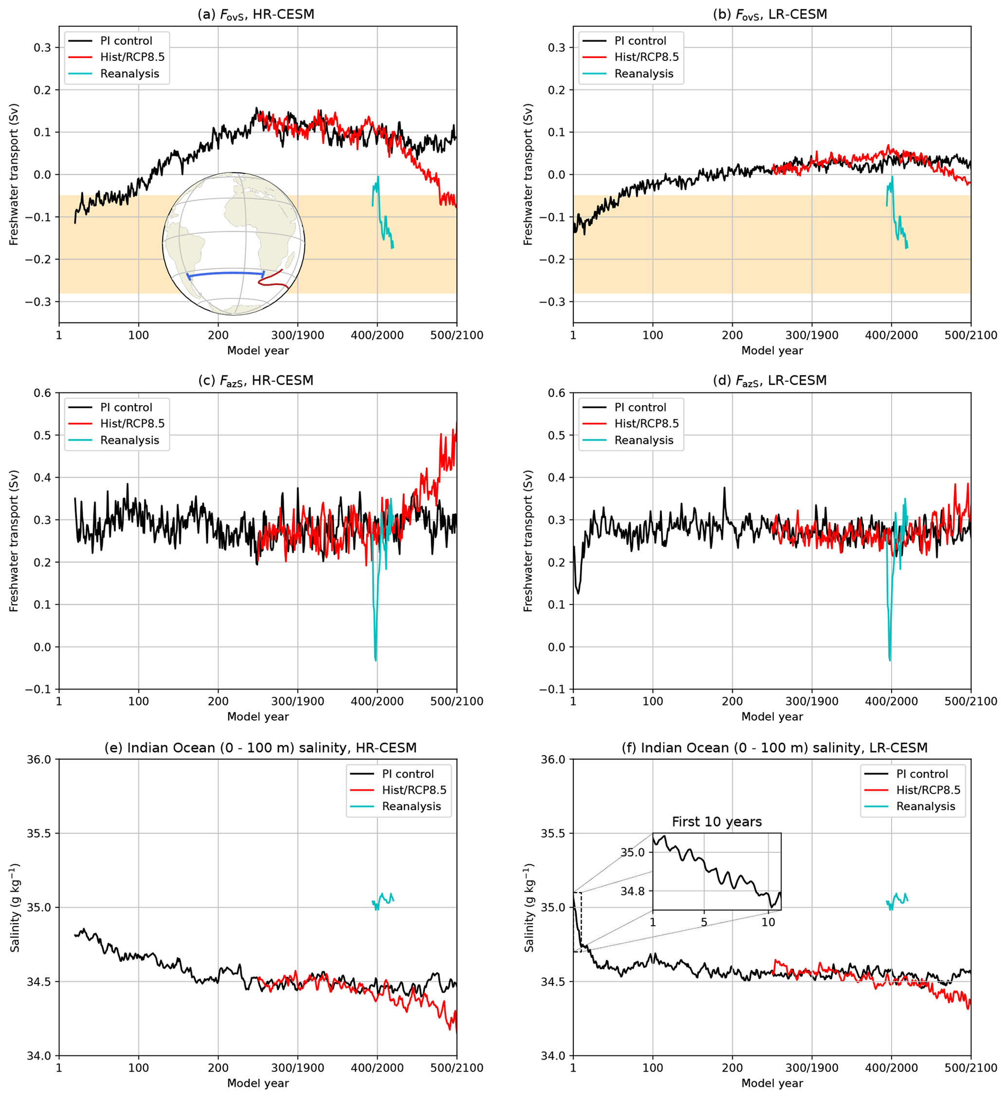
Figure 1 (a, b) The freshwater transport by the overturning component at 34° S, F_ovS, for the (a) HR-CESM and (b) LR-CESM. The cyan-coloured curve shows the reanalysis. The yellow shading indicates observed ranges (Garzoli et al., 2013; Mecking et al., 2017). The inset in panel (a) shows the region of interest, including the section at 34° S (blue) and a schematic representation of the Agulhas Current and Retroflection (red). (c, d) Similar to panels (a) and (b) but now for the azonal (gyre) component, F_azS. (e, f) The vertically averaged (0–100 m) and spatially averaged salinity over the Indian Ocean for the (e) HR-CESM and (f) LR-CESM, including reanalysis. The inset in panel (f) shows the volume-averaged salinity over the first 10 years (monthly averages).

The upper 500 m salinity fields at 34° S are (strongly) influenced by Agulhas Leakage, and the water properties of the leakage have an Indian Ocean origin. The upper 100 m Indian Ocean strongly freshens by 0.3 g kg⁻¹ in the first 10 years for the LR-CESM (Fig. 1f). For the HR-CESM this is only 0.2 g kg⁻¹ in the first 20 years (Fig. 1e), where we used the initial value of the LR-CESM for reference. The relatively large adjustment of the upper 100 m Indian Ocean salinities induces the temporal response in F_azS in the LR-CESM. It is possible that the HR-CESM shows a similar response, but this can not be verified. The quantity F_azS reaches an equilibrium state much faster compared to the F_ovS. The AMOC also imports the relatively fresh water of Indian Ocean origin into the Atlantic basin, and this contributes to the drift in F_ovS.

To better quantify the water mass contributions to F_ovS changes, we separate the total F_ovS over the four different water masses, and each contribution is shown in Fig. 2. The F_ovS drift mainly originates from the ASW and the NADW water masses for both the HR-CESM and LR-CESM. The AAIW and AABW contributions show adjustments in the first 50 model years and then remain fairly constant over the remaining simulation period. The ASW contribution to the F_ovS drift is related to the strong freshening of the Indian Ocean. The upper Indian Ocean's freshening manifests itself within a decade; these are typical timescales of atmospheric adjustment, while oceanic adjustments typically take much longer time. Indeed, there is a strong precipitation response over the Indian Ocean which contributes to the freshening of the Indian Ocean; changes in evaporation are much smaller (not shown). These precipitation responses over the Indian Ocean are likely related to Intertropical Convergence Zone (ITCZ) biases (Mamalakis et al., 2021). The Indonesian Throughflow also imports more (net) fresh water into the Indian Ocean (not shown), but this can not solely explain the (strong) freshening of the Indian Ocean in the first decade of the LR-CESM. The negative salinity anomalies (with respect to initialisation) in the Indian Ocean eventually reach the Agulhas Retroflection and through the Agulhas Leakage affect the upper 500 m salinity fields at 34° S (i.e. the ASW). This leads to positive freshwater anomalies transported into the Atlantic Ocean which contribute to the F_ovS drift.

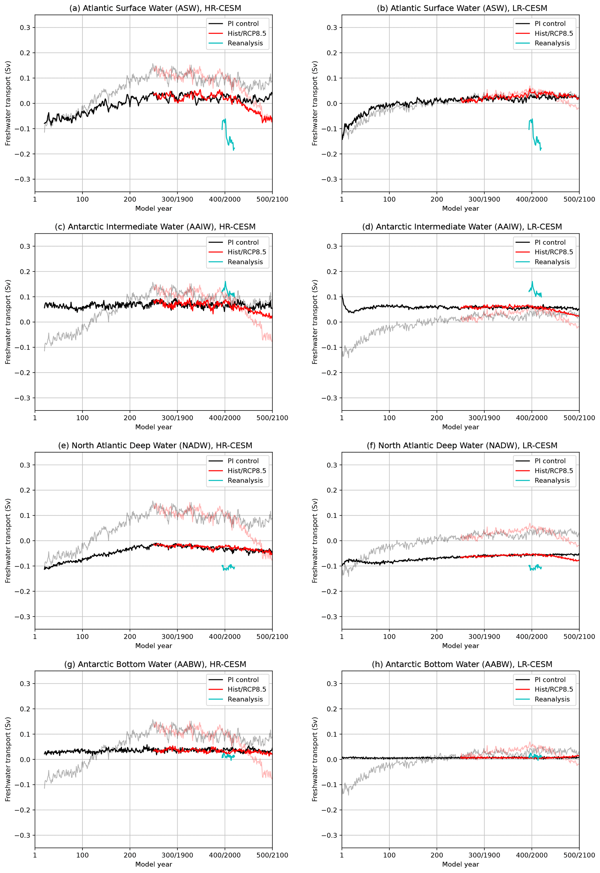
Figure 2 The F_ovS contributions for the four different water masses for the HR-CESM (a, c, e, g) and LR-CESM (b, d, f, h). The cyan-coloured curve shows the reanalysis. The opaque curves show the freshwater transport by the overturning component, F_ovS (see also Fig. 1a and b).

The NADW also contributes to the F_ovS drift (Fig. 2e and f). The NADW is part of the southward-flowing limb of the AMOC, and this water mass originates from deep water formation at the higher latitudes in the North Atlantic. This motion in this water mass is linked to the AMOC strength, which is shown in Fig. 3a and b. There is some adjustment in the first 100 model years of the PI control simulations (AMOC is 0 Sv at initialisation), but thereafter it is in near equilibrium. The adjustment in AMOC strength during the first 100 years results in sea surface temperature (SST, insets in Fig. 3a and b) responses. These SST responses induce surface salinity anomalies mainly through evaporation (not shown). These surface salinity anomalies undergo deep water transformation over the Labrador basin, Irminger basin, or Iceland basin (i.e. regions of deep convection) and influence the salinities over these three basins at depth (1000–3000 m, Fig. 3c and d).

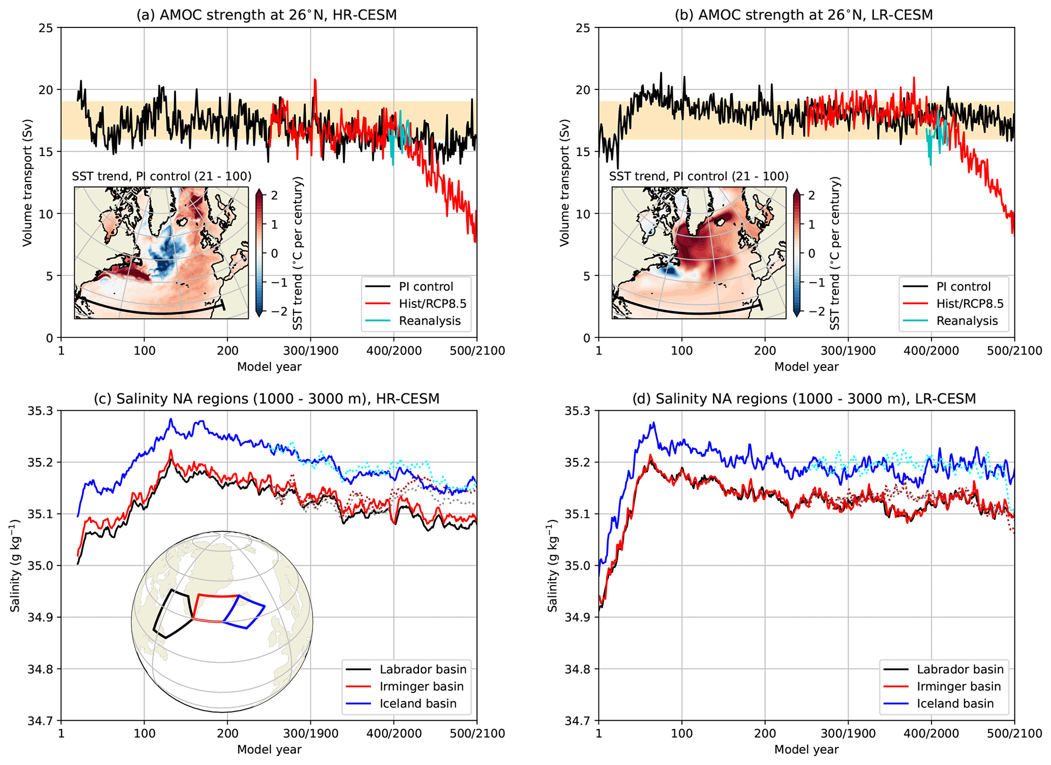
Figure 3 (a, b) The AMOC strength at 1000 m and 26° N (determined at black section in inset) for the (a) HR-CESM and (b) LR-CESM. The cyan-coloured curve shows the reanalysis. The yellow shading indicates observed ranges (Smeed et al., 2018; Worthington et al., 2021). Inset: the SST trend (PI control, model years 21–100). (c, d) The vertically averaged (1000–3000 m) and spatially averaged salinity over the Labrador basin, Irminger basin and Iceland basin (see inset in panel c) for the (c) HR-CESM and (d) LR-CESM. The solid (dotted) curves indicate the PI control (Hist/RCP8.5) simulation.

The AMOC responses and related SST responses (Caesar et al., 2018) in the first 100 years are the opposite when comparing the HR-CESM and LR-CESM. The positive SST trends in the LR-CESM enhance evaporation and result in more saline surface waters at the higher latitudes compared to the HR-CESM. The surface salinities at the higher latitudes also increase in the HR-CESM (mainly over the East and West Greenland Current) but at a lower rate due to the reduced evaporation through lower SSTs. The different surface salinity changes are also reflected in the timing of the salinity maxima over the three deep convection basins, which are around model year 65 for the LR-CESM and around model year 130 for the HR-CESM. The AMOC strength has a local maximum around the same years for the respective model. After the salinity maxima there is a gradual decrease in the salinity content over the three basins for both models, while the AMOC also declines by 0.5 Sv per century (p<0.01, model years 130–500) for the HR-CESM and by 0.2 Sv per century (p<0.01, model years 130–500) for the LR-CESM.

The newly formed water mass in the three deep convection basins takes about 100 years to reach 34° S and then influence the NADW properties there. One expects a larger change in the NADW properties for the LR-CESM as the deep water formation salinity responses are about twice as strong in the LR-CESM than in the HR-CESM (during the first 100 model years). Yet, the NADW contribution to F_ovS changes (Fig. 2e and f) shows a stronger drift (model years 100–250) in the HR-CESM (0.038 Sv per century, p<0.01) than the LR-CESM (0.014 Sv per century, p<0.01). The differences in the NADW freshwater transport trends are related to the ventilation rate of the NADW. By analysing the average water age of the NADW (not shown) we find that the NADW is ventilated faster in the HR-CESM than the LR-CESM. This larger ventilation rate is related to the high horizontal ocean model resolution in the HR-CESM, resulting in much more eddy-induced horizontal mixing (with respect to the LR-CESM). After model year 250, the NADW freshwater transport slightly declines again (−0.011 Sv per century, p<0.01) in the HR-CESM, which is consistent with the salinity maxima in the Labrador basin, Irminger basin and Iceland basin that are reached 100 years earlier. Over this later period, the LR-CESM shows a persistent positive NADW trend (0.004 Sv per century, p<0.01) which contributes to the drift in F_ovS. This indicates that the salinity content of the deeper ocean in the LR-CESM takes a much longer time to adjust than the HR-CESM, in particular given that the salinity maxima of the Labrador basin, Irminger basin and Iceland basin are reached around model year 65 for the LR-CESM.

The Atlantic's northern boundary (at 60° N, F_ovN) also contributes to the freshwater budget of the Atlantic Ocean, and the convergence/divergence of fresh water by the overturning circulation is indicated by $\mathrm{\Delta }{F}_{\text{ov}}=F_{\text{ovS}}-F_{\text{ovN}}$ (Dijkstra, 2007; Weijer et al., 2019). For the HR-CESM PI control, F_ovN is about −0.03 Sv, and its magnitude is smaller than F_ovS (Fig. 4a), and hence ΔF_ov≈F_ovS. For the LR-CESM PI control, F_ovN contributes quite some more to ΔF_ov (Fig. 4b). As a result, the values of ΔF_ov are fairly similar for the HR-CESM and LR-CESM between model years 200–500.

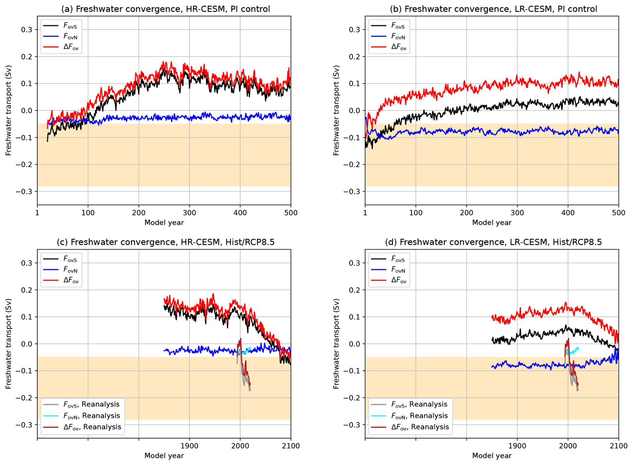
Figure 4 The freshwater transport by the overturning component at 34° S (black curve, F_ovS), 60° N (blue curve, F_ovN) and the freshwater convergence (red curve, $\mathrm{\Delta }{F}_{\text{ov}}=F_{\text{ovS}}-F_{\text{ovN}}$) for the PI control (a, b) and Hist/RCP8.5 (c, d) simulations. The reanalysis is displayed in the lower row. The yellow shading indicates observed ranges for the F_ovS.

3.2 The present-day comparison

In the previous subsection we analysed the onset of the F_ovS drift in the PI control simulations. Some quantities, such as the F_azS and the AAIW, showed some adjustments in the first 50 years, but those changes hardly contributed to the F_ovS drift. However, these quantities can have various biases when comparing this to present-day observations (i.e. reanalysis). To systematically compare the available reanalysis data (1994–2020) with the CESM, we analyse the same model years 1994–2020 from the Hist/RCP8.5 simulations. The Hist/RCP8.5 simulations are indicated by the red-coloured curves and reanalysis by the cyan-coloured curves (Figs. 1 through 3).

There are indeed large biases in the patterns of ASW, AAIW and NADW in the Hist/RCP8.5 simulations. Whereas the meridional velocities at 34° S are reasonably simulated (Fig. 5a–c), the ASW is too fresh, in particular in the eastern part of the Atlantic (Fig. 5d–f). The relatively fresh ASW is related to the surface salinities over the Indian Ocean which are too fresh (−0.5 g kg⁻¹) when comparing the Hist/RCP8.5 simulations with reanalysis (Fig. 1e and f). On the other hand, the positive surface salinity anomalies in the North Atlantic, which undergo deep water transformation, result in a too salty NADW. The Hist/RCP8.5 simulations consequently have a positive F_ovS bias upon initialisation and during the years 1994–2020. The F_azS and AMOC strength are reasonably simulated in both the HR-CESM and LR-CESM. The F_azS in the reanalysis shows large variations before the year 2000, which is due to internal variability in the zonal salinity variations over the upper 500 m.

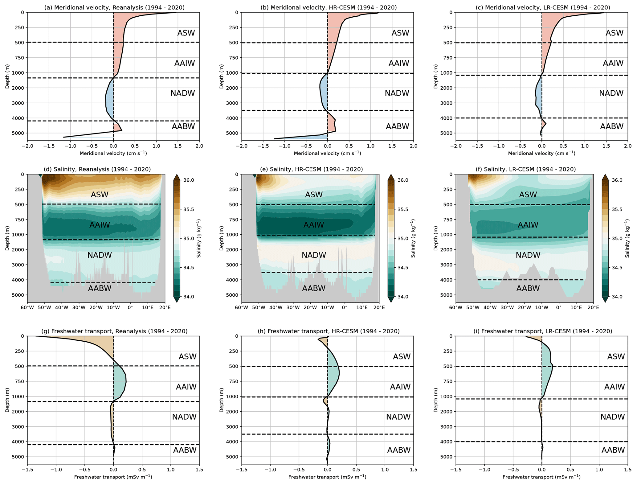
Figure 5 (a–c) The present-day (1994–2020) zonally averaged meridional velocity at 34° S. (d–f) The present-day (1994–2020) salinity along 34° S. (g–i) The present-day (1994–2020) freshwater transport with depth at 34° S. The present-day profiles originate from reanalysis and the HR-CESM and LR-CESM under the Hist/RCP8.5 forcing scenario. Note that the vertical axis is cropped below 1000 m depths.

The AAIW originates from the Antarctic Convergence zone (near 50–60° S) and submerges when flowing northward, as shown in Fig. 6. In the HR-CESM, the shape (not the absolute values) and outcropping of the isopycnals resemble that of the reanalysis, and the pattern of the AAIW is well represented in the HR-CESM. The zonal velocities, which are related to the Antarctic Circumpolar Current (near 50° S), are slightly higher in the HR-CESM than in the reanalysis. The shape and outcropping of the isopycnals are substantially different in the LR-CESM when comparing those to the reanalysis. The outcropping in the LR-CESM occurs further south, giving rise to different water mass properties of the AAIW. The ventilation of the AAIW is not that well resolved in the LR-CESM, and this results in a relatively saline AAIW compared to the reanalysis and HR-CESM (Fig. 5). The relatively saline AAIW and the too weak meridional velocities (at 34° S) explain why the AAIW bias is larger in the LR-CESM than in the HR-CESM.

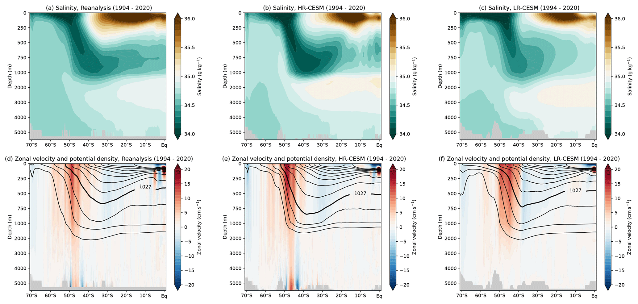
Figure 6 (a–c) The present-day (1994–2020) and zonally averaged (50° W–20° E, Atlantic sector) salinity. (d–f) The present-day (1994–2020) and zonally averaged (50° W–20° E, Atlantic sector) zonal velocity (shading) and potential density (contours are the isopycnals); the contours are each spaced by 0.25 kg m⁻³, where the thick contour is 1027 kg m⁻³ for reference. The present-day profiles originate from reanalysis and the HR-CESM and LR-CESM under the Hist/RCP8.5 forcing scenario. Note that the vertical axis is cropped below 1000 m depths.

The biases in the three water masses ASW, NADW and AAIW result in freshwater transport biases at 34° S (Fig. 5g–i), but the biases in the ASW and NADW are the most dominant and induce a positive F_ovS bias. The contribution of the AABW is fairly small, and hence we do not discuss it here. The value of F_ovN has a small contribution (−0.027 Sv, 1994–2020) to the freshwater convergence ΔF_ov in the reanalysis. In the HR-CESM, the value of F_ovN (−0.030 Sv, 1994–2020) is close to the reanalysis, but for the LR-CESM (−0.080 Sv, 1994–2020) it is a factor 3 larger than in the reanalysis (Fig. 4). This shows that ΔF_ov≈F_ovS(34° S) in both the reanalysis and in the HR-CESM.

3.3 Climate change simulations

The present-day comparison between reanalysis and the CESM simulations shows biases in various oceanic quantities. There are also differences when comparing the HR-CESM and LR-CESM biases, which are likely related to the different horizontal resolutions between the two models. The oceanic responses under climate change are substantially different when analysing high-resolution and low-resolution climate models (van Westen et al., 2020; van Westen and Dijkstra, 2021), and such a response can also be expected for the freshwater transport at 34° S (Jüling et al., 2021). In this subsection we investigate the freshwater transport responses under the Hist/RCP8.5 scenario (model years 2000–2100).

The presented quantities in Figs. 1 through 4 for the Hist/RCP8.5 simulations remain close to their PI control simulations under the historical forcing (1850–2005) but start to deviate in the last 100 years of the simulation. The values of F_ovS decrease under climate change (model years 2000–2100, Fig. 1a and b) for both the HR-CESM (−0.19 Sv per century, p<0.01) and LR-CESM (−0.076 Sv per century, p<0.01). Changes in F_ovS can be induced by AMOC changes and/or by salinity changes. The AMOC weakens over the entire Atlantic Ocean and reduces the zonally averaged meridional velocity magnitudes in the northward-flowing branch (upper 1000 m) and southward-flowing branch (1500–4000 m), as shown in the insets in Fig. 7e and f at 34° S. The AMOC strength (Fig. 3a and b) decreases by −8.2 Sv per century (p<0.01) and −8.9 Sv per century (p<0.01) for the HR-CESM and LR-CESM simulations, respectively.

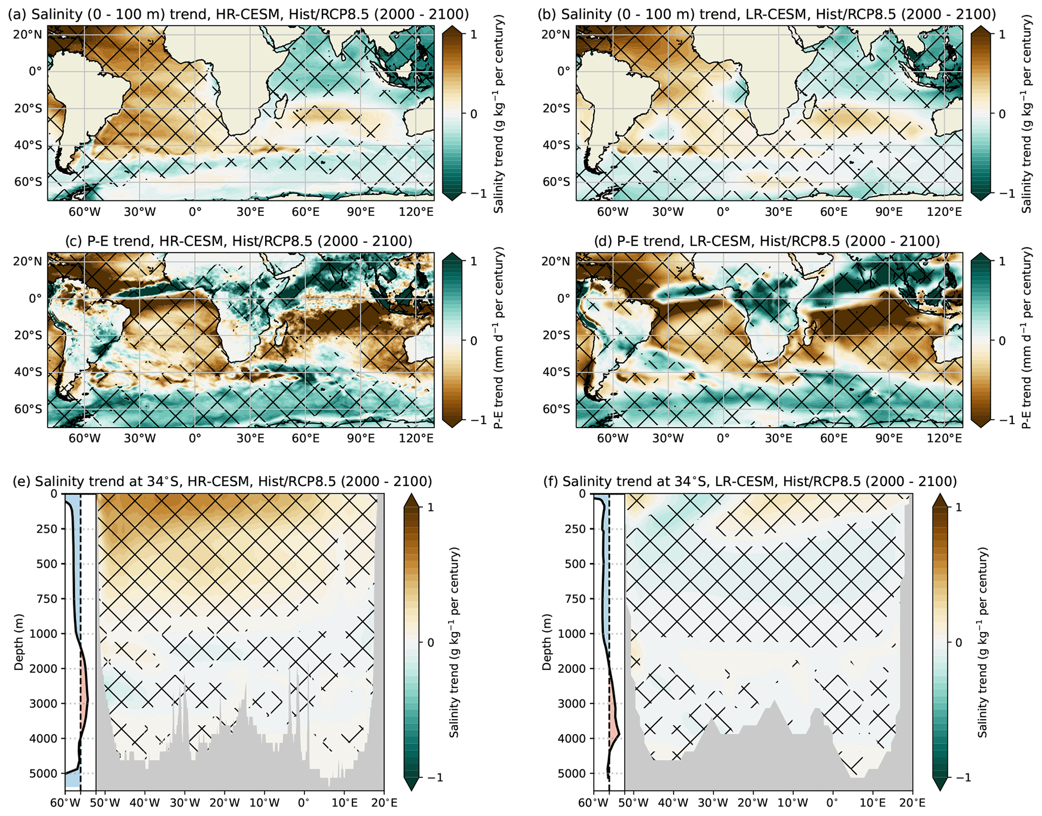
Figure 7 (a, b) The vertically averaged (0–100 m) salinity trends (Hist/RCP8.5, model years 2000–2100) for the (a) HR-CESM and (b) LR-CESM. (c, d) The P–E trends (Hist/RCP8.5, model years 2000–2100) for the (c) HR-CESM and (d) LR-CESM. (e, f) The salinity trends (Hist/RCP8.5, model years 2000–2100) along 34° S for the (e) HR-CESM and (f) LR-CESM. Inset: the zonally averaged meridional velocity trend at 34° S; the horizontal ranges are between −0.2 and 0.2 cm s⁻¹ per century. The hatched regions in all panels indicate significant (p<0.05) trends. Note that the vertical axis is cropped below 1000 m depths for panels (e) and (f).

The vertically averaged (0–100 m) salinity in the Atlantic Ocean increases under climate change, which is related to negative P–E trends (induced by higher evaporation rates through higher SSTs) over the Atlantic (Fig. 7a–d). Changes in the South American monsoon result in more precipitation over the South Atlantic Ocean (near 30° S). These changes are the strongest in the LR-CESM, leading to a surface freshening around 30° S and 30° W. The upper 100 m salinity over the Indian Ocean decreases by about 0.17 g kg⁻¹ per century (p<0.05) for both the HR-CESM and LR-CESM, but there is a south–north dipole pattern in both salinity and P–E trends. The northward ITCZ shift over the Indian Ocean leads to a different precipitation pattern and results in positive salinity trends in the southern part of the Indian Ocean and, from this, in the Agulhas Leakage (Fig. 7e and f). The azonal (gyre) component F_azS increases under climate change (Fig. 1c and d), and these changes are mainly induced by altering the zonal salinity gradient along the 34° S section, in particular near the surface (0–250 m depths). In both the HR-CESM and LR-CESM, this near-surface salinity gradient increases under climate (compare the salinity trends between the western and eastern part of the section), and this is most pronounced in the HR-CESM. The relatively saline water in the western part of the section is advected out of the Atlantic (via the Brazil Current), resulting in an F_azS increase. The F_azS trends are 0.21 Sv per century (p<0.01) and 0.09 Sv per century (p<0.01) for the HR-CESM and LR-CESM, respectively.

The salinity response at intermediate depths (250–1000 m) at 34° S is the opposite for the HR-CESM and LR-CESM (Fig. 7e and f) simulations. As discussed in the previous subsection, the outcropping of the isopycnals is different between the HR-CESM and LR-CESM, and the outcropping latitude occurs further south in the LR-CESM (somewhere in the centre of the Weddell Gyre). Changes in the surface water properties near the Weddell Gyre are therefore connected to the AAIW changes in the LR-CESM. The surface salinity trends over Weddell gyre are mainly negative (i.e. freshening) in the LR-CESM, whereas there are both positive and negative salinity trends in the HR-CESM. The primarily negative salinity trends in the LR-CESM are related to another ocean bias: a too strong stratification in the Southern Ocean. The strong stratification prevents (deep) vertical mixing of relatively saline water towards the surface (van Westen and Dijkstra, 2020). The melting of sea ice and snow (on top of the sea ice) under climate change contribute to the freshening of the Weddell Gyre in the absence of (deep) vertical mixing in the LR-CESM. The Southern Ocean stratification and (deep) vertical mixing are much better resolved in a high-resolution model (van Westen and Dijkstra, 2020) and explain the different salinity trends near the Weddell Gyre between the HR-CESM and LR-CESM. The salinity responses (at 34° S) below 1000 m are much smaller and less zonally coherent compared to the upper 1000 m. The climate change response is delayed at greater depth (by about 100 years), which explains the differences in salinity trends between the upper 1000 m and those below 1000 m depth. Salinity changes in the deep water formation regions in the North Atlantic have only a limited effect within this 100-year period (model years 2000–2100).

For the HR-CESM, the ASW and AAIW are the main contributors (53.9 % and 29.5 %, respectively) to the F_ovS trend under climate change (Fig. 2). The more saline ASW and AAIW water masses are the dominant factor in the F_ovS response. The lower zonally averaged meridional velocities as a consequence of AMOC weakening slightly reduce the magnitude of the ASW and AAIW trends. For the LR-CESM, the ASW, AAIW and NADW contribute 23.7 %, 51.3 % and 35.4 % to the F_ovS trend, respectively (note that the AABW contributes −10.4 %). The lower meridional velocities induce the negative ASW and AAIW freshwater responses, as these water masses become fresher over time. The negative NADW contribution is related to a freshening of this water mass, and this freshening is partly related to changes in the vertical extent of the NADW (it extends into the relatively fresh AAIW over time). The AAIW, NADW and AABW contributions to the F_ovS trend are 58.6 %, 20.6 % and −2.9 % when fixing the vertical NADW extent to 1000–4000 m, respectively; the ASW contribution remains unaltered. This effect of the varying NADW extent is smaller in the HR-CESM (12.8 % for varying and 7.4 % for fixed NADW). Although the F_ovS decreases in both the HR-CESM and LR-CESM, the F_ovS response is due to different processes, where it is mainly salinity dominated in the HR-CESM and overturning dominated in the LR-CESM.

3.4 CMIP6 model results

The systematic comparison between the HR-CESM and LR-CESM results clearly show the differences in the F_ovS values and the associated water masses, which are mainly related to the horizontal resolutions between the model configurations. To investigate whether these biases occur also in other models, we include an analysis of F_ovS using 39 different CMIP6 models (under the Hist/SSP5-8.5 scenario). Details about the CMIP6 models used are provided in Table A1.

In Fig. 8 we present the F_ovS (components) and AMOC strength for the 39 CMIP6 models, together with the HR-CESM, LR-CESM and reanalysis. First we compare all the models against the present-day (1994–2020) reanalysis (left column in Fig. 8). We categorise the models in four different categories: models with a realistic present-day F_ovS (diamond markers, 13 CMIP6 models), models with a realistic present-day AMOC strength (circled markers, 7 CMIP6 models), models with both a realistic present-day F_ovS and AMOC strength (hexagon markers, 0 CMIP6 models), and the remaining models (crossed markers, 19 CMIP6 models). None of the CMIP6 models (and the HR-CESM and LR-CESM) have both a realistic present-day F_ovS and realistic AMOC strength, and only the reanalysis falls within this category. The 26 CMIP6 models with a positive F_ovS bias compared to observations have a stronger AMOC strength compared to the 13 models with a realistic F_ovS (mean AMOC strength of 17.4 and 12.6 Sv, respectively). Similar to the HR-CESM and LR-CESM, most of the F_ovS bias can be explained by the ASW and NADW contributions (Fig. 8c and g).

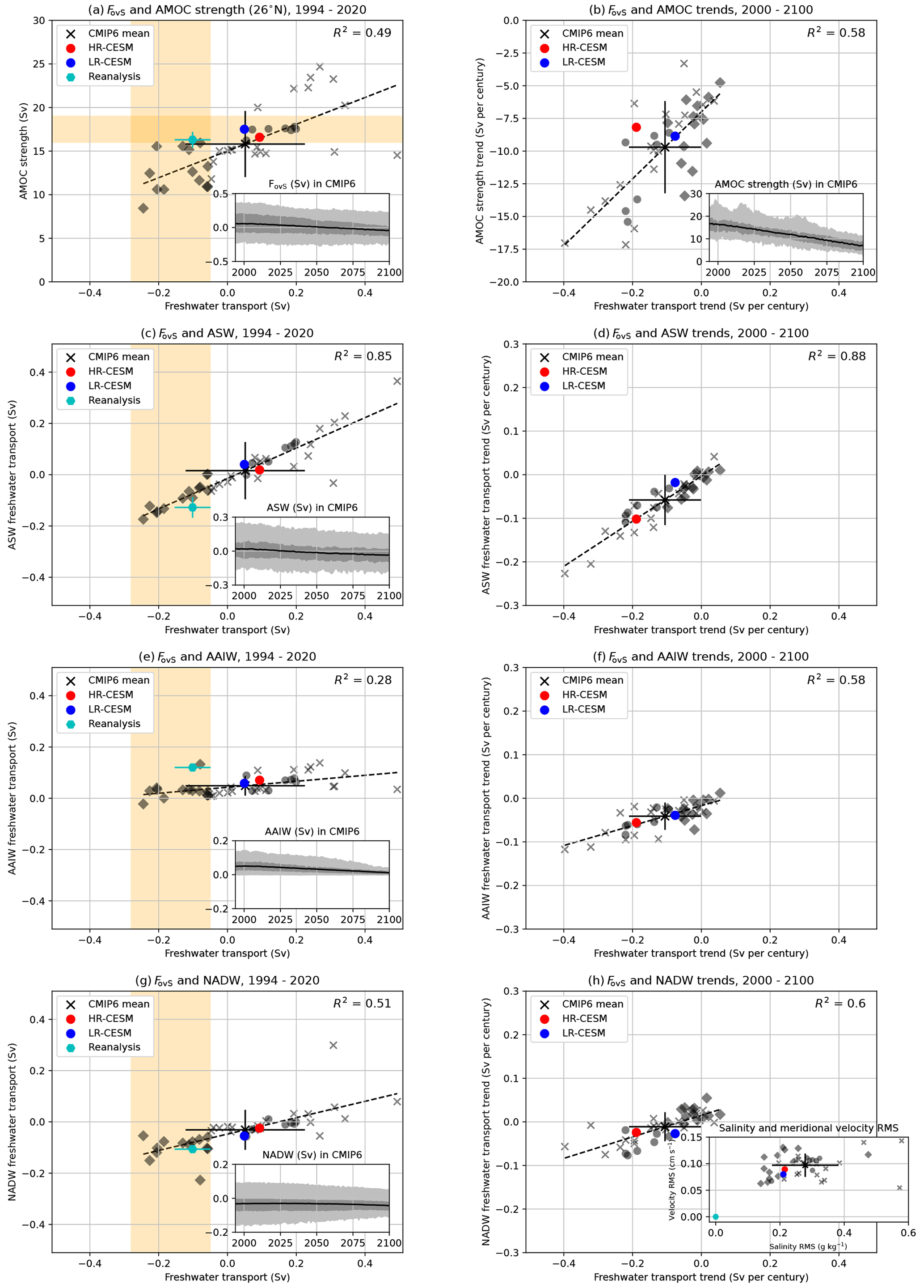
Figure 8 (a, c, e, g) The present-day (model years 1994–2020) freshwater transport by AMOC (at 34° S, F_ovS) and (a) AMOC strength (at 26° N and 1000 m), (c) ASW freshwater transport contribution, (e) AAIW freshwater transport contribution and (g) NADW freshwater transport contribution for CMIP6, HR-CESM, LR-CESM and reanalysis. The individual CMIP6 models are indicated in grey. The diamond and circle markers have a realistic (i.e. within a yellow band) F_ovS and AMOC strength, respectively, whereas the cross markers fall outside the yellow bands. Hexagon markers have both a realistic F_ovS and AMOC strength. (b, d, f, h) Similar to panels (a), (c), (e) and (g) but for the trends (model years 2000–2100) in the freshwater transport (components) and AMOC strength. The insets in panels (a), (b), (c), (e) and (g) show the CMIP6 model mean (black line) and CMIP6 model variance (50 % and 95 % confidence levels, shading) for the freshwater transports and AMOC strength over time. The inset in panel (h) shows the model deviations with respect to reanalysis for the present-day salinity section and zonally averaged (baroclinic) meridional velocity profile (at 34° S), here expressed as the weighted root-mean-square errors. The CMIP6 model mean and model standard deviation are also indicated in all panels. The dashed lines in all panels indicate the CMIP6 model regression; the R² value is indicated in the top-right corner.

For the 13 CMIP6 models with a realistic F_ovS, only four of them (CNRM-CM6-1, CNRM-ESM2-1, MCM-UA-1-0 and MRI-ESM2-0) have a reasonable present-day AMOC strength (≈15.5 Sv), but the remaining ones have a fairly weak AMOC strength (<13.3 Sv). The CNRM-CM6-1, CNRM-ESM2-1 and MRI-ESM2-0 are relatively fresh (with respect to reanalysis) near 10° W and the surface, which results in a positive freshwater bias for the ASW, but this is compensated for by a smaller AAIW contribution. This relatively fresh bias appears (to some extent) in most of the CMIP6 models (Fig. A1) and also in the HR-CESM and LR-CESM (Fig. 5). The displayed CMIP6 profiles in Fig. A1 are somewhat small and should only be used for pattern comparison. The freshwater bias near the surface is smaller in the MCM-UA-1-0 and is the one model closest to the reanalysis for the AAIW freshwater contribution (Fig. 8e). However, for the MCM-UA-1-0 the positive ASW freshwater bias is compensated for by a stronger NADW freshwater export out of the Atlantic Ocean. It is interesting that the MCM-UA-1-0 is relatively close to the reanalysis, given that this model has the lowest ocean resolution among the analysed models (Table A1). There are seven CMIP6 models with a strong positive freshwater bias (F_ovS>0.2 Sv), and these models (e.g. FGOALS-f3-L, GISS-E2-2-G, TaiESM1) have an unrealistic mean state at 34° S. There is only one model (MCM-UA-1-0) which is close to the reanalysis for the AAIW contribution (Fig. 8e), and most models underestimate the AAIW contribution.

The MCM-UA-1-0 appears to be the model closest to observations and reanalysis, but this qualification changes when determining the present-day salinity and zonally averaged meridional velocity root-mean-square errors (RMSEs) with respect to reanalysis at 34° S (inset in Fig. 8h). The MCM-UA-1-0 has the second largest salinity RMSE and second largest velocity RMSE of all the diamond-labelled models (i.e. realistic F_ovS). The diamond-labelled models have on average the smallest salinity biases (relatively low salinity RMSE) of the CMIP6 suite, but regarding the velocity RMSE they are not considerably better than the other CMIP6 models because the diamond-labelled models have a relatively weak AMOC. The FGOALS-g3 has the lowest velocity RMSE, but this model has an unrealistic salinity profile and relatively strong AMOC strength (23.3 Sv) when comparing to the reanalysis. These results underline that having a realistic F_ovS does not imply a realistic present-day mean state.

Similar to the CESM results, we find decreasing values in F_ovS (and its components) and AMOC strength under climate change (Fig. 8b, d, f, and h). The 13 CMIP6 models with a realistic present-day F_ovS show a much smaller F_ovS trend (−0.022 Sv per century) than in the remaining 26 CMIP6 models (−0.15 Sv per century). The ASW response is the dominant contributor in the F_ovS trend. Note that these F_ovS trends can either be salinity driven (as in the HR-CESM) or overturning driven (as in the LR-CESM).

The HR-CESM and LR-CESM results are consistent with the CMIP6 results, and the CESM simulations are actually close to the CMIP6 mean (Fig. 8). Most CMIP6 models and the CESM simulations are too fresh near the surface at 34° S (i.e. the ASW contribution), resulting in a positive freshwater F_ovS bias compared to observations. Models with a realistic F_ovS have biases in either the AAIW contribution, NADW contribution or AMOC strength. None of the models analysed here has a realistic present-day mean state when compared to available observations and reanalysis.

4 Summary and discussion

Our analysis of CMIP6 models and high-resolution (HR) and low-resolution (LR) versions of the CESM has shown that persistent biases in these models remain in the AMOC-induced Atlantic freshwater transport, as measured by F_ovS. The values of F_ovS from the reanalysis product (which is steered towards observations) are in good agreement with those from direct observations (Bryden et al., 2011; Garzoli et al., 2013). In the climate model simulations, numerous processes contribute to this deficiency in F_ovS: ITCZ positioning and strength, Agulhas Leakage, Indonesian Throughflow, AMOC strength, and ventilation of the AAIW and NADW. Biases in the ASW induce the most dominant F_ovS biases and occur on relative short timescales (years). Biases in the NADW also induce F_ovS biases but occur on longer (decadal-to-centennial) timescales.

Several model studies (Small et al., 2014; Jüling et al., 2021; van Westen et al., 2020; van Westen and Dijkstra, 2021) demonstrated oceanic bias reductions when increasing the horizontal resolution in the ocean model. However, here the F_ovS bias is larger in the HR-CESM PI control than the LR-CESM PI control (after model year 150). This larger bias is related to a faster (oceanic) adjustment in the higher horizontal resolution model, which allows for more eddy-induced horizontal mixing ventilation. The freshwater convergence/divergence (ΔF_ov) is, however, fairly similar in HR-CESM and LR-CESM, which is related to a relatively large contribution of F_ovN in the LR-CESM. The ASW freshwater transport is fairly similar between the HR-CESM and LR-CESM PI control, but this contribution is mainly related to the Indian Ocean's surface (0–100 m) salinity and is influenced by precipitation and the Indonesian Throughflow. These results suggest that increasing the ocean model horizontal resolution would have a limited impact on F_ovS biases as these biases are strongly controlled by those in the atmospheric model component.

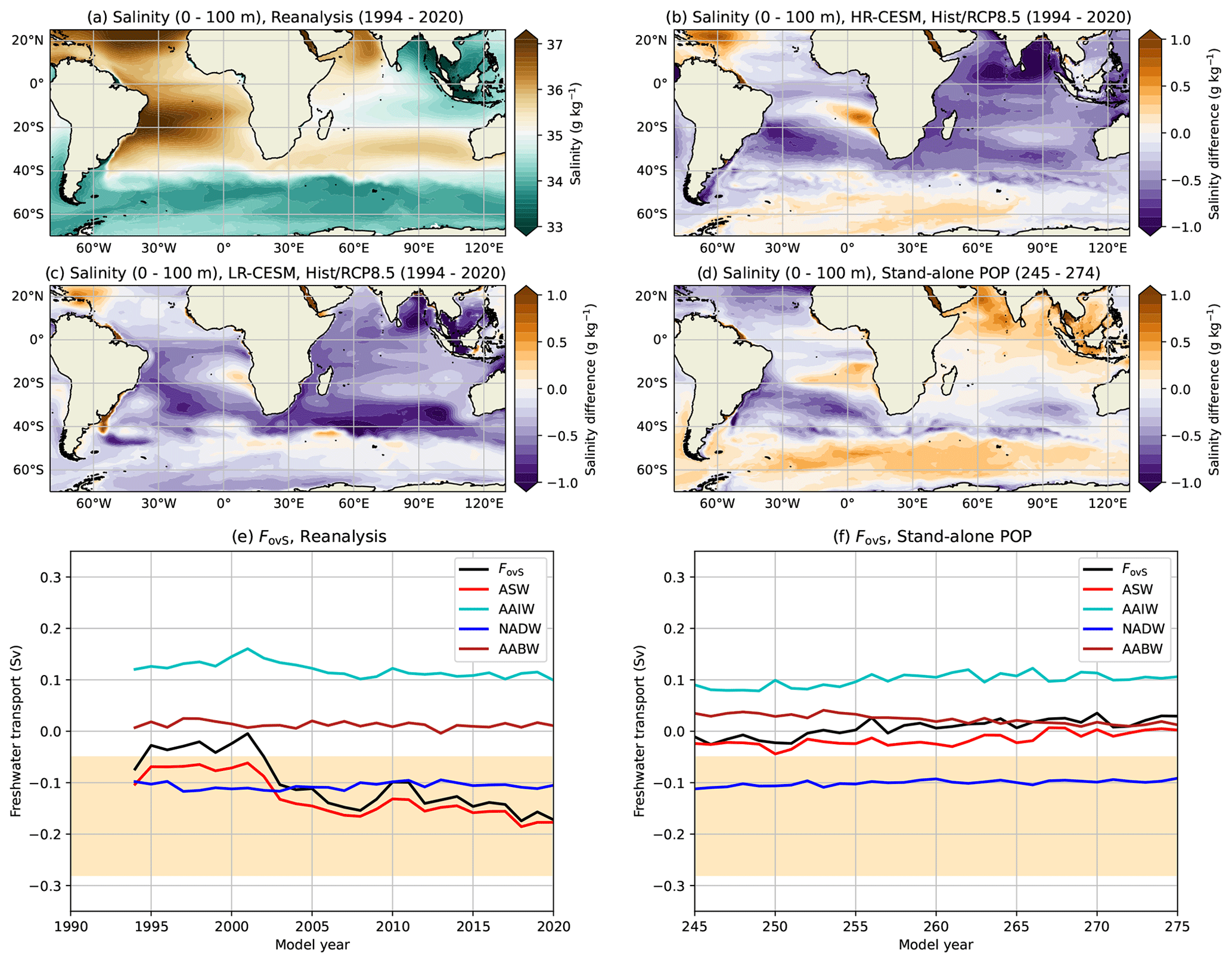
Figure 9 (a–d) The present-day (1994–2020) and vertically averaged (0–100 m) salinity for (a) reanalysis, (b) HR-CESM and (c) LR-CESM. For the (d) stand-alone POP the time mean of model years 245–274 is shown. For the HR-CESM, LR-CESM and stand-alone POP, the salinity differences compared to the reanalysis are displayed, where the reanalysis data are re-gridded onto each model grid. (e, f) The freshwater transport at 34° S and its components for (e) reanalysis and the (f) stand-alone POP; the time series for the HR-CESM and LR-CESM are already shown in Fig. 2.

To further explore the influence of atmospheric freshwater biases on F_ovS, we have conducted simulations with only the ocean component of the CESM (i.e. the Parallel Ocean Program, POP) with the prescribed Coordinated Ocean-Ice Reference Experiment (CORE, derived from observations) forcing dataset (Large and Yeager, 2004; Weijer et al., 2012; Le Bars et al., 2016). The surface (0–100 m) salinity biases are substantially reduced in the Indian Ocean in the stand-alone POP simulation (0.1° horizontal resolution) and hence reduce the ASW biases (Fig. 9). The NADW in the stand-alone POP remains close to the reanalysis after 250 years of model integration, whereas the NADW in the HR-CESM PI control simulation has strongly drifted over this period (Fig. 2e). This indicates that the atmospheric component and fluxes need to be improved in the coupled climate simulations to have a realistic salinity distribution, specifically in the Indian Ocean. Once in coupled interaction with the other model components, this would likely then reduce the biases in the Atlantic Surface Water component of F_ovS.

The biases in F_ovS due to atmospheric biases are found not only in CESM, but in a large number of CMIP6 models. The CMIP6 model mean has a positive F_ovS bias which is similar to that in the CMIP5 results (Mecking et al., 2017). Values of F_ovS decrease under climate change in both versions of the CESM, but the changes are salinity driven in the HR-CESM, while for the LR-CESM the changes are overturning driven. Most of the CMIP6 models have similar biases to those in the CESM. The models with a realistic F_ovS have biases elsewhere; for example, their F_ovS contributions of the AAIW and their AMOC strengths are underestimated. The bottom line is that CMIP6 models either have a too weak present-day AMOC or have a wrong sign of F_ovS.

In state-of-the-art climate models, such as in the latest CMIP6 models, the AMOC weakens under future climate change (Weijer et al., 2020; van Westen et al., 2020) but no (abrupt) AMOC collapses are found. However, it is questionable whether these climate models are fit for purpose to determine the risk of AMOC tipping, because of their biases identified here and mainly the wrong sign of F_ovS. The absence of AMOC tipping can be connected to the results from idealised climate models (Dijkstra, 2007; Huisman et al., 2010), which suggest that the AMOC is in its monostable (bistable) regime when F_ovS is positive (negative). However, there has been substantial criticism on this aspect of F_ovS (Gent, 2018; Mignac et al., 2019; Haines et al., 2022). For example, Haines et al. (2022) show that in 10 CMIP5 models the variations in F_ovS do not influence the AMOC strength. However, the AMOC strength in these models poorly matches with that from observations, likely related to a coarse (>1°) horizontal ocean resolution. The AMOC in EC-Earth3 and MPI-ESM1-2-HR does not show transition behaviour (Jackson et al., 2023) under the chosen forcing scenario while having a slightly negative F_ovS (Table A1). These two CMIP6 models also have a relatively weak AMOC strength (<14 Sv), a too fresh ASW and a too saline NADW. These biases likely influence the salt–advection feedback strength and hence the AMOC responses. In Gent (2018) it is stated that the wind-driven salinity transport is not taken into account properly when the AMOC strength varies. However, as argued in Weijer et al. (2019), the wind-driven transport is ineffective in changing the salinity in the Atlantic as a whole and hence does not control the stability of the AMOC. Atmospheric feedbacks, such as the shift of the ITCZ due to AMOC, are not accounted for in F_ovS, but the available model studies (Den Toom et al., 2012; Castellana and Dijkstra, 2020) have indicated that these effects are small. While this issue is far from settled, if F_ovS<0 is indeed an indicator for the existence of a multi-stable AMOC regime, then models with F_ovS>0 grossly underestimate the probability that an AMOC collapse can occur.

The results presented in this study show persistent freshwater transport biases in the latest state-of-the-art climate models. The resulting effect of these biases is that the major salt–advection feedback is not adequately represented. This leads to an underestimation of AMOC weakening under climate change and freshwater forcing experiments and likely reduces the probability of AMOC tipping. Because such AMOC weakening and/or tipping can disrupt society worldwide within a few decades, it is very urgent for model biases to be reduced so that proper estimates of tipping probabilities can be obtained.

Appendix A

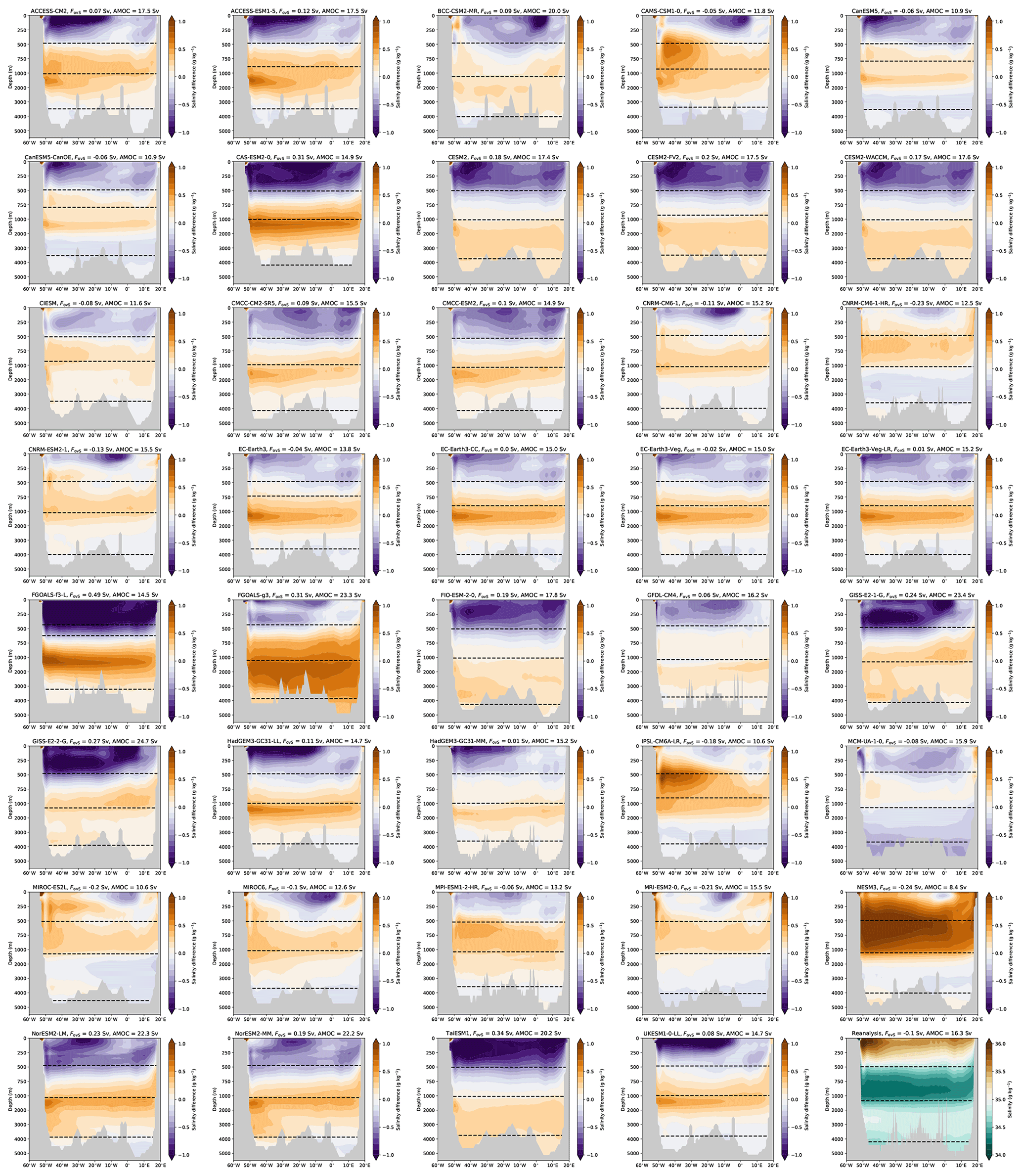
Figure A1 The present-day (1994–2020) salinity at 34° S for the 39 CMIP6 models and reanalysis (lower right). For CMIP6, the salinity differences compared to the reanalysis are displayed, and the reanalysis data are regridded onto each CMIP model grid. The present-day (1994–2020) F_ovS and AMOC strength (1000 m and 26° N) are displayed at the top of each panel. The dashed lines indicate the different water masses (top to bottom: ASW, AAIW, NADW and AABW). Note that the vertical axis is cropped below 1000 m depths.

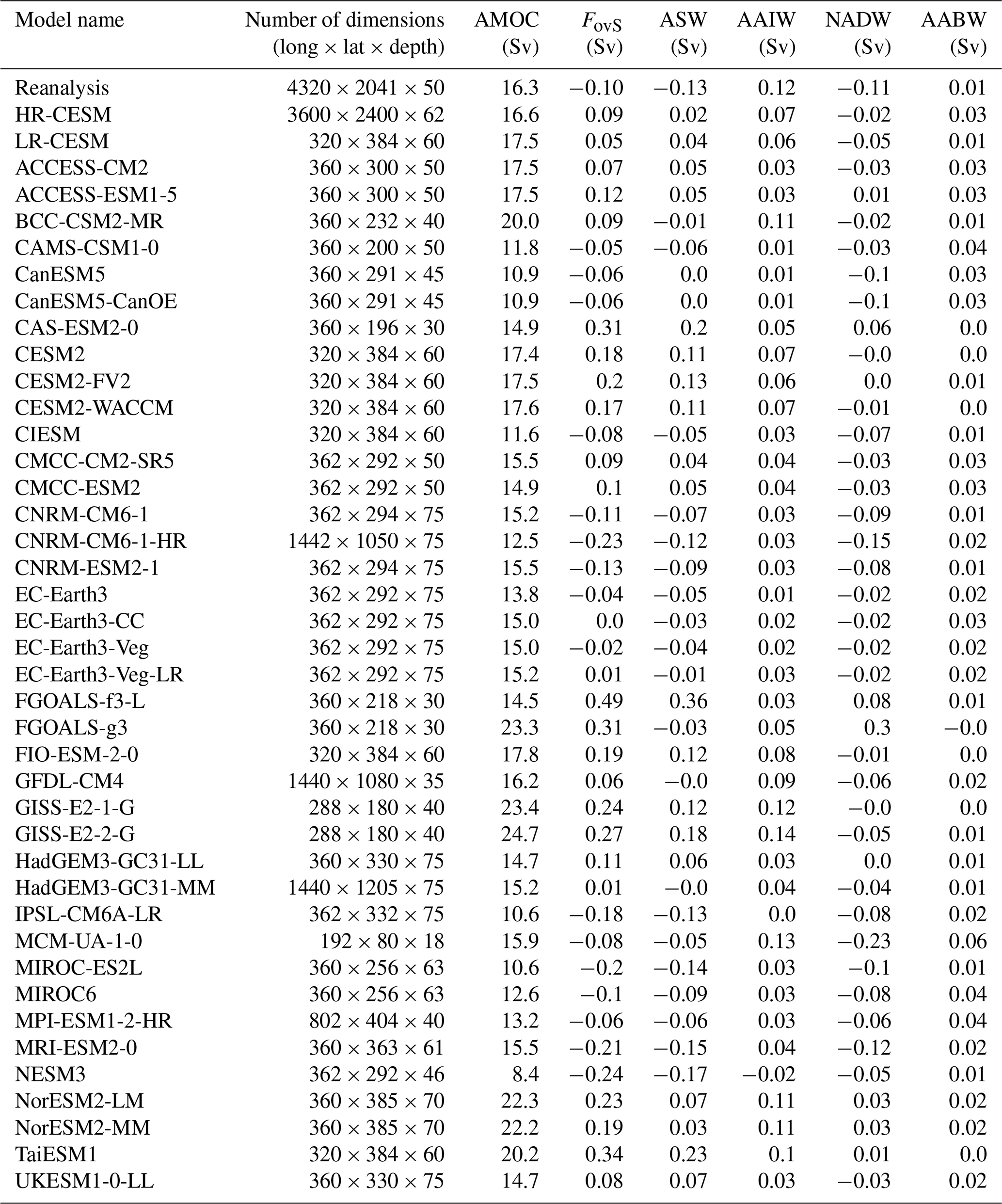
Table A1 The models used in this study with the dimensions of the ocean component, the AMOC strength and the F_ovS (contributions) for the present-day period (1994–2020).