Global variability of high-nutrient low-chlorophyll regions using neural networks and wavelet coherence analysis

We examine 20 years of monthly global ocean color data and modeling outputs of nutrients using self-organizing map (SOM) analysis to identify characteristic spatial and temporal patterns of high-nutrient low-chlorophyll (HNLC) regions and their association with different climate modes. The global nitrate-to-chlorophyll ratio threshold of NO₃ : Chl > 17 (mmol NO₃ mg Chl⁻¹) is estimated to be a good indicator of the distribution limit of this unproductive biome that, on average, covers 92 × 10⁶ km² (∼ 25 % of the ocean). The trends in satellite-derived surface chlorophyll (0.6 ± 0.4 % yr⁻¹ to 2 ± 0.4 % yr⁻¹) suggest that HNLC regions in polar and subpolar areas have experienced an increase in phytoplankton biomass over the last decades, but much of this variation, particularly in the Southern Ocean, is produced by a climate-driven transition in 2009–2010. Indeed, since 2010, the extent of the HNLC zones has decreased at the poles (up to 8 %) and slightly increased at the Equator (< 0.5 %). Our study finds that chlorophyll variations in HNLC regions respond to major climate variability signals such as the El Niño–Southern Oscillation (ENSO) and Meridional Overturning Circulation (MOC) at both short (2–4 years) and long (decadal) timescales. These results suggest global coupling in the functioning of distant biogeochemical regions.

1 Introduction

High-nutrient low-chlorophyll (HNLC) areas are ocean regions where primary production should be potentially high but phytoplankton biomass remains relatively low and constant despite the perennial nutrient availability for growth (Martin and Fitzwater, 1988; Chisholm and Morel, 1991). They are interesting regions because they challenge the accepted paradigm of a positive relation between macronutrient concentrations and phytoplankton biomass in open waters but, most importantly, because they represent an important fraction of the global ocean carbon inventories, and therefore their extent influences the potential withdrawal of atmospheric CO₂ to the deep ocean (Martin et al., 1990; De Baar et al., 1995; Boyd et al., 2005). It is estimated that HNLC biomes cover roughly between 20 % and 30 % of the world's oceans, comprising three major ocean areas: the subarctic North Pacific (SNP), the eastern equatorial Pacific (EEP), and most of the Southern Ocean (SO) (Martin, 1990; Coale et al., 1996; Parekh et al., 2005).

Because nitrogen is the mineral nutrient needed in greatest abundance by phytoplankton and owing to its generalized depletion in surface waters over much of the oceans, it is considered a key limiting nutrient for ocean production. In HNLC regions, where nitrogen is in excess, other non-exclusive factors such as rapid top-down control by zooplankton grazing, low irradiance, limitations by silicic acid availability, and/or iron (Fe) limitation have been hypothesized to explain the persistently low chlorophyll (Chl). While these factors may contribute to different degrees to the observed low Chl and determine the phytoplankton dynamics in HNLC regions (see Chavez et al., 1991; Cullen, 1995; Coale et al., 1996; Dugdale and Wilkerson, 1998; Landry et al., 2011), it is generally acknowledged that Fe availability is central to the productivity of HNLC regions (Boyd et al., 2007). All HNLC regions share a chronic Fe depletion in surface waters, and experimental results show highly positive productivity responses to Fe addition (Martin et al., 1994; Boyd et al., 2000, 2004; Tsuda et al., 2003; Coale et al., 2004). Indeed, Fe requirements are the largest among the trace metals for several metabolic processes, and not surprisingly, it has been considered the ultimate limiting nutrient (Moore and Doney, 2007). This has led to the proposal of a conceptual model of phytoplankton nutrient limitation in the modern ocean based on two functioning regimes: one in which the supply of nutrients is relatively slow with nitrogen availability limiting productivity and a complementary regime, with enhanced macronutrient supply, wherein Fe limits productivity (Moore et al., 2013).

Iron limitation influences the uptake of nitrogen, thereby explaining the unused nitrate concentrations in HNLC regions. Indeed, it has been proposed that a delicate balance between nitrogen and Fe availability modulates phytoplankton growth and that co-limitation is rather ubiquitous in the sea (Bryant, 2003; Browning et al., 2017). Other elements and compounds such as B vitamins, which are also scarce in Fe-limited areas, can also be co-limiting factors for phytoplankton growth in these regions (e.g., Koch et al., 2011; Bertrand et al., 2012). For example, it has been experimentally shown that the addition of Fe and B12 to Antarctic phytoplankton assemblages can synergistically increase phytoplankton growth (Bertrand et al., 2011; Cohen et al., 2017).

Despite their relevance for global ocean productivity and carbon fluxes, HNLC regions remain loosely defined, and knowledge of their temporal and spatial variability and trends is limited. Moreover, their response in a global warming scenario is uncertain. Only general aspects such as expected shifts in phytoplankton community composition and changes in Fe-cycling rates have been addressed to date (Fu et al., 2016; Lauderdale et al., 2020). The original description of HNLC systems by Minas et al. (1986) referred to a slowly growing phytoplankton standing stock despite the presence of high nutrient concentrations. However, there are no rigid criteria accurately defining the functioning of these ecosystems. Several ecosystem characteristics such as species composition, ecosystem structure, carbon utilization pathways, and response to climate change also differ between the HNLC and other ecosystems, reflecting differences in the limiting factor (Falkowski et al., 1998; Ono et al., 2008).

Of particular interest are the aspects related to the reduced variability and high permanence (i.e., temporal persistence) typically characterizing large HNLC regions. These features are distinctive from those of highly variable systems, which may temporarily present HNLC conditions. For example, some light-limited regions at high latitudes may present low productivity and enhanced nutrients during winter, but they respond to a transient situation that does not correspond to the generally accepted HNLC paradigm. Similarly, high nutrients and low Chl have been observed at the end of the spring bloom in some productive systems (Nielsdóttir et al., 2009; Birchill et al., 2019) and some areas located in coastal upwelling regions (Hutchins et al., 1998, 2002; Firme et al., 2003; Eldridge et al., 2004). While complying with the necessary conditions of high nutrients and low Chl, it is uncertain whether these ephemeral systems share structural and functional similarities with the large HNLC regions.

At a time when understanding biogeochemical responses to large-scale forcings, including climate change, has become a scientific priority, it seems appropriate to revisit some concepts of the functioning of HNLC regions. Their extent and variability are indicative of the dynamic changes in the bidirectional interrelationships of phytoplankton with the environment and with other organisms at large scales. Most of the information on the long-term variations of HNLC regions is drawn from global studies suggesting that their productivity is varying as a consequence of global warming and that they experience prominent interannual to decadal fluctuations superimposed on these long-term trends (i.e., Boyce et al., 2014; Martinez et al., 2020). Available evidence suggests that some HNLC regions may be decreasing in size as a result of increased ocean stratification (Ono et al., 2008). More recently, Yasunaka et al. (2016) determined that surface trends of phosphate and silicate in the North Pacific are associated with the shoaling of the mixed layer, reporting that surface nutrient concentration was correlated with the North Pacific Gyre Oscillation (NPGO). Some studies have shown that oligotrophic areas in the Northern Hemisphere are expanding (e.g., Polovina et al., 2008); however, with some exceptions (i.e., Radenac et al., 2012; Yasunaka et al., 2014), specific long-term studies on HNLC regions are scarce, and knowledge of their variability on the global ocean scale and their responses to climate change remains uncertain.

The objective of the present study is to provide a quantitative assessment of the large-scale patterns of variability of the three major HNLC regions (SNP, EEP, and SO) and their relationship with the main modes of climate variability. Systematically determining the boundaries of these HNLC regions has remained elusive since it requires coherent information on nutrients and Chl fields. The present study is based on the analysis of 20-year time series of monthly global ocean color data and nutrient concentrations from a biogeochemical model using machine learning techniques and wavelet analysis. First, based on the statistical analysis of global NO₃ : Chl ratios, we determine a robust quantitative criterion to objectively define HNLC regions. Then we characterize the temporal variability patterns of HNLC regions based on their NO₃ and Chl concentrations by using the self-organizing map (SOM) technique. We use the herein-established statistical criterion to assess the spatial variations of HNLC regions over the study period unveiled from the SOM analysis in the spatial domain of NO₃ : Chl ratios. Finally, through a combined SOM–wavelet coherence analysis (WCA), we quantify the spectral power and the dynamic relationship between the observed Chl variability and two main global-scale forcings: the El Niño–Southern Oscillation (ENSO) and Meridional Overturning Circulation (MOC). We show that the combination of WCA with SOM-derived characteristic time series is an especially suitable tool for the analysis of driver–response relationships in the ocean.

2 Materials and methods

2.1 Ocean color data

We employ 20 years of monthly global composites of satellite Chl Level-3 products, derived from merging SeaWiFS, MERIS, MODIS AQUA, and VIIRS sensors using a Garver–Siegel–Maritorena (GSM) algorithm (Maritorena and Siegel, 2005), obtained from the GlobColour dataset (https://www.globcolour.info, last access: 12 June 2023). The chlorophyll product is spatially gridded, and the weighted average of the different merged Level-2 products is then calculated. The composite consists of a rectangular regular map product in degrees with a spatial resolution of 0.25^∘ (i.e., around 28 km at the Equator) and covers the period from January 1998 to December 2017. We excluded results in the Arctic Ocean and the coastal Southern Ocean due to the interference of ice cover and prolonged gaps in the data. A total of 654 395 pixels were considered in the analysis. We are aware that the consistency of merged multi-mission ocean color satellite series may suffer from some limitations, influencing long trend analysis (Mélin et al., 2017). However, no significant increase or decrease is observed in the first-order trends of GlobColour data in more recent studies (e.g., Moradi, 2021). Therefore, while recognizing that some differences in regional and seasonal biases may occur in unified data products and acknowledging that discontinuities and trends of the median with time should be interpreted carefully according to the sensors used (Garnesson et al., 2019), merged Chl can be generally considered a good indicator of the magnitude of the overall phytoplankton trends.

2.2 Nitrate data

Since nutrient observations are still too scarce to allow obtaining time-resolved global-scale fields, we used global NO₃ obtained from the biogeochemical hindcast model provided by Mercator-Ocean (http://marine.copernicus.eu, last access: 12 June 2023, see Fig. S1 in the Supplement). It consists of monthly mean fields of several biogeochemical variables at 0.25^∘ horizontal resolution over the global ocean obtained using the PISCES model (Aumont et al., 2015). The model is forced by daily mean fields of ocean, sea ice, and atmospheric conditions. Ocean and sea ice forcings are obtained from the numerical simulation FREEGLORYS2V4 produced at Mercator-Ocean and the source of atmospheric forcings is the ERA-Interim reanalysis produced at ECMWF. Initial conditions are set from the World Ocean Atlas 2013 climatology. A complete model description can be found at https://doi.org/10.48670/moi-00019. We compared available observational nutrient data (NO₃) from the sea surface (mean 0–20 m), obtained by merging bottle-cast data from the World Ocean Database (WOD18, Boyer et al., 2018; https://www.nodc.noaa.gov/, last access: 12 June 2023) with model results. Generally, we found good agreement between nitrate in situ data and model results (r=0.98). Main deviations occur in the Southern Ocean where NO₃ concentrations are overestimated (up to 7.2 mmol m⁻³).

2.3 Climatological data

Data on climate indices were obtained from available databases. The Bi-monthly Multivariate El Niño–Southern Oscillation Index (MEI.v2), hereafter the ENSO index, was obtained from the National Oceanic and Atmospheric Administration National Center for Environmental Prediction website (https://www.esrl.noaa.gov/psd/enso/mei/, last access: 12 June 2023). MOC data (Moat et al., 2022; Smeed et al., 2019) for the period (2004–2018) were obtained from the RAPID-WATCH MOC monitoring project (https://www.rapid.ac.uk/rapidmoc, last access: 12 June 2023).

2.4 Identification of HNLC regions

Presently, the best approximation to define the global distribution of HNLC regions in the world ocean is the use of National Oceanographic Data Center (NODC) maps of surface nutrients (https://www.nodc.noaa.gov/, last access: 12 June 2023). However, excess nutrient availability by itself does not necessarily reflect HNLC conditions. In situ experiments are capable of discerning Fe limitation conditions, but a more manageable metric to assess the limits on the spatial extent of HNLC regions is required, in particular for remote sensing applications, as well as for allowing objective comparison between different environmental scenarios and studies.

To obtain a quantitative criterion for the definition of HNLC regions, we analyze the values of NO₃ : Chl ratios (mmol mg⁻¹) obtained from the SOM analysis on the time domain over the global ocean throughout the 20 years of data to identify a common statistical behavior representing HNLC conditions. In particular, we use the probability density function (PDF) of the extracted SOM NO₃ : Chl temporal patterns to identify a threshold for defining HNLC conditions (P_HNLC). Changes in the trend of the standard deviation calculated for each bin of the PDF function are employed to set a threshold ratio. To calculate the total extent of each region (km²), the spatial area of each pixel was calculated by considering its latitude.

2.5 Time and space domain SOM analyses

We use SOM (Kohonen, 1982) to elucidate spatial and temporal patterns in the complex relationship between nutrients and phytoplankton. SOM is a subtype of artificial neural network that uses an unsupervised machine learning algorithm to process and extract hidden structures in large datasets. The SOM algorithm is mainly based on a training process through which an initial neural network is transformed by iteratively presenting the input data. In this study, the architecture of the neural network is set in a sheet hexagonal map lattice of neurons, or units, to have equidistant neurons and to avoid anisotropy artifacts. Each neuron is represented by a weight vector with a number of components that is equal to the dimension of the input data vector, i.e., the number of rows or columns in the Chl and NO₃ matrices, depending on whether the analysis is performed in either the temporal or spatial domain. We use an initial network composed of units of random values (random initialization). In each successive iteration during the training process, the neuron with the greatest similarity (excited neuron), called the best-matching unit (BMU), is updated by replacing its values with the Chl and NO₃ values of the input sample data. The similarity is estimated by computing the Euclidean distance between the components of the input sample and the components of the weight vector of the unit. The unit most similar to the input sample is the one with the minimum distance. In the learning process, Chl and NO₃ values of the topological neighboring neurons of the excited neuron (BMU) are also updated by replacing their values with values determined by a Gaussian neighborhood function. In these computations, we use the imputation batch training algorithm (Vatanen et al., 2015), whereby the SOM assumes that a single sample of data (input vector) contributes to the creation of more than one pattern, as the whole neighborhood around the best-matching pattern is also updated in each step of training. This yields a more detailed assimilation of particular features appearing on neighboring patterns. A final neural network with the NO₃ : Chl patterns is obtained after repeating the training process until a stable convergence of the map is obtained.

For typical satellite datasets, the SOM can be applied to both space and time domains. By applying the SOM in the spatial domain, one can extract characteristic spatial patterns of the input data. If transposing the input data matrix and applying the SOM in the time domain, one can extract characteristic temporal patterns, i.e., the characteristic time series. Since each of these time series represents the temporal variability of a particular region, this method can be used to identify regions of differentiated variability on a map. The SOM, when applied to both space and time domains of the same data (called “dual SOM” analysis by Liu et al., 2016), provides a powerful tool for diagnosing ocean processes from these different perspectives. In this study, we focus on the second type. We have addressed the analysis separately in the time and space domains of the log-transformed NO₃ and Chl datasets. In the time domain, we implement a [4×3] joint-SOM analysis of NO₃ and Chl using as input weight vectors concatenating the time series of NO₃ and Chl at each pixel, so each neuron corresponds to a characteristic joint NO₃ and Chl temporal pattern over the total period of data. Since each pixel has an associated characteristic time series, we can obtain the location of a particular temporal pattern by computing the BMU for each pixel, providing a map of regions of differentiated NO₃ : Chl temporal variability. For the analysis presented herein only the regions with NO₃ : Chl > P_HNLC are considered (regions R1 to R5).

An obstacle to the temporal domain analysis on a global scale is the opposed seasonality in both of Earth's hemispheres. The algorithm classifies the time series at each grid point corresponding to the period of the signal but does not consider time lags between the time series. Hence, pixels located in either the Northern or Southern Hemisphere displaying a similar significant period in the NO₃ and Chl temporal variability are classified in the same regional pattern even if they are in antiphase when the signals are seasonally lagged (6-month delay). Regionalization is spatially coherent, but the seasonal variation in the characteristic pattern that represents the neuron mixes the phenological patterns of both hemispheres. Therefore, to properly analyze the properties and trends of each of the classified regions, we have calculated the mean features of the regions by segregating the grid points corresponding to each pattern obtained from the SOM analysis into the Northern Hemisphere, Equator, and Southern Hemisphere (see scheme in Fig. 1). Linear trends of NO₃ and Chl concentrations in each region are estimated by decomposing the NO₃ : Chl time series in a seasonal signal plus a residual component and applying Theil–Sen slope adjustment (Sen, 1968) of the residuals of the deseasonalized series. Correlation analyses were performed using the Pearson product moment correlation, computing best-fit linear trends using regression analysis.

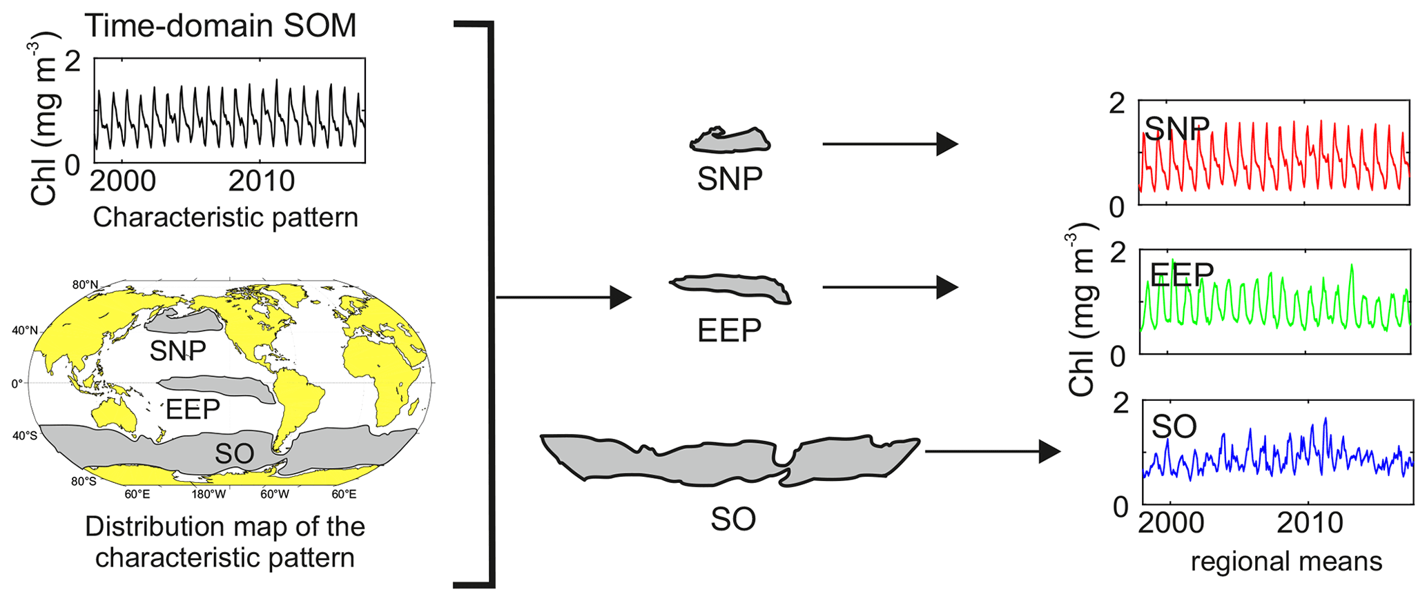
Figure 1 Scheme of a characteristic pattern and its distribution map obtained from SOM time domain analysis, as well as global and regional mean series calculated for each of the HNLC regions.

The SOM analysis in the spatial domain [3×3] array is addressed by using as input data weighted vectors consisting of spatial distributions over the global ocean of NO₃ : Chl ratios at a particular time. The selection of the number of neurons depends on the complexity of the data, the features to be examined in the dataset, and the minimization of the errors. In this case, the resulting neurons after the training loop unveil the characteristic patterns describing the spatial variability of the HNLC regions on a global scale. Then, when computing the BMU for each time we designate the extracted characteristic spatial pattern that better describes the spatial distribution of NO₃ : Chl ratios (P1 to P9) at each time, obtaining the time evolution of the characteristic spatial patterns throughout the considered period.

Because the SOM is based on the similarity computed from the Euclidean distance between samples, the input vectors of the different variables are normalized to the same range before initializing the SOM computations. This guarantees a consistent comparison of the weights of the components when computing the distance of two vectors.

The size of the neural network (number of neurons) depends on the number of samples and the complexity of the patterns. An optimal choice is important to maximize the quality of the SOM. In the present study, the map size is set to [4×3] with 12 neurons for the time domain analysis, and a [3×3] neural network is used in the spatial domain. Using larger map sizes, the patterns are slightly more detailed, and more regions of a particular variability emerge, but the occurrence of the probability of the patterns decreases, without affecting the results noticeably (Basterretxea et al., 2018; Hernández-Carrasco and Orfila, 2018). If a reduced neural map, such as [2×2], is used, patterns are concentrated together with the occurrence probability in a few rough patterns, but in this case increasing the topological error.

SOM computations have been performed using the MATLAB© toolbox of SOM v.2.0 (Vesanto et al., 1999) provided by the Helsinki University of Technology (http://www.cis.hut.fi/somtoolbox/, last access: 12 June 2023). Further information on SOM analysis is provided in the Supplement.

2.6 Combined SOM–wavelet coherence analysis

Joint SOM–wavelet power spectral analysis was demonstrated by Liu et al. (2016) in the study of characteristic time series of sea level variations in different regions of the Gulf of Mexico. Here, we expand it further to combined SOM–wavelet coherence analysis to assess the response of HNLC regions to global forcings. We use an approach based on the wavelet coherence analysis (WCA) between two time series (Grinsted et al., 2004; see the Supplement for further details). WCA characterizes cross-correlations by identifying the main frequencies, phase differences, and time intervals over which the relationship between the variability of HNLC regions and the main global forcings considered in this study, ENSO and MOC indexes, is strong. To do so, we first analyze the variability in both frequency and time of the characteristic time series of NO₃ : Chl in the different HNLC regions extracted by the time domain SOM computations and the time series of the global forcings using the continuous wavelet transform (CWT).

Cross-wavelet transform (XWT) characterizes the association between the CWT of two signals, providing information on the common power and relative phase in the frequency–time domain of two time series. By applying the XWT to the NO₃ : Chl ratios and climate forcings, we determine the cyclic changes in each of the HNLC regions and their relationship with the global forcings mentioned above. Finally, we quantify the correlation between the continuous wavelet transform of two signals using the wavelet coherence analysis (WCA). In the time–frequency space the wavelet coherence coefficient R² is calculated as the squared absolute value of the smoothed cross-wavelet spectrum normalized by the product of the smoothed wavelet individual spectra for each scale (Torrence and Compo, 1998; Torrence and Webster, 1999; Grinsted et al., 2004). R² is interpreted as a localized correlation coefficient in the frequency–time domain, and it takes values between 0 (no correlation) and 1 (perfect correlation). The statistical significance level of the wavelet coherence is estimated using Monte Carlo methods as described in Grinsted et al. (2004). We use the MATLAB software package (Grinsted et al., 2004) for wavelet coherence analysis. It should be noted that cross-wavelet analysis does not establish causative relationships but only allows identifying possible linkages between variables through the synchrony of their time series.

3 Results

3.1 Global characterization of HNLC regions

The mean pattern of global ocean color data for the 20 years analyzed reveals the well-known contrast in phytoplankton biomass between the highly productive areas located at high latitudes as well as in coastal upwelling regions and the low-latitude oceanic waters, where mean values are <0.1 mg m⁻³ (Fig. 2). Low-Chl regions generally correspond to low surface NO₃ concentrations, whereas the opposite relationship (high nitrate and high chlorophyll) is more exceptional. Indeed, nutrient-rich productive waters are mainly restricted to shelf regions (coastal upwelling regions and shelf seas) or to the vicinity of islands (i.e., Falkland Islands) and other topographical features where multiple and overlapping sources of other elements, such as trace metals, are abundant (e.g., Pollard et al., 2009; Boyd and Ellwood, 2010). As shown in Fig. 2, only in the North Atlantic, the Bering Sea, and the eastern region of the Antarctic Peninsula is Chl enhanced. Conversely, a large part of surface ocean waters, particularly in the Southern Ocean and in the equatorial Pacific, corresponds to regions of relatively low Chl concentrations but with excess nitrate (i.e., >4 mmol m⁻³).

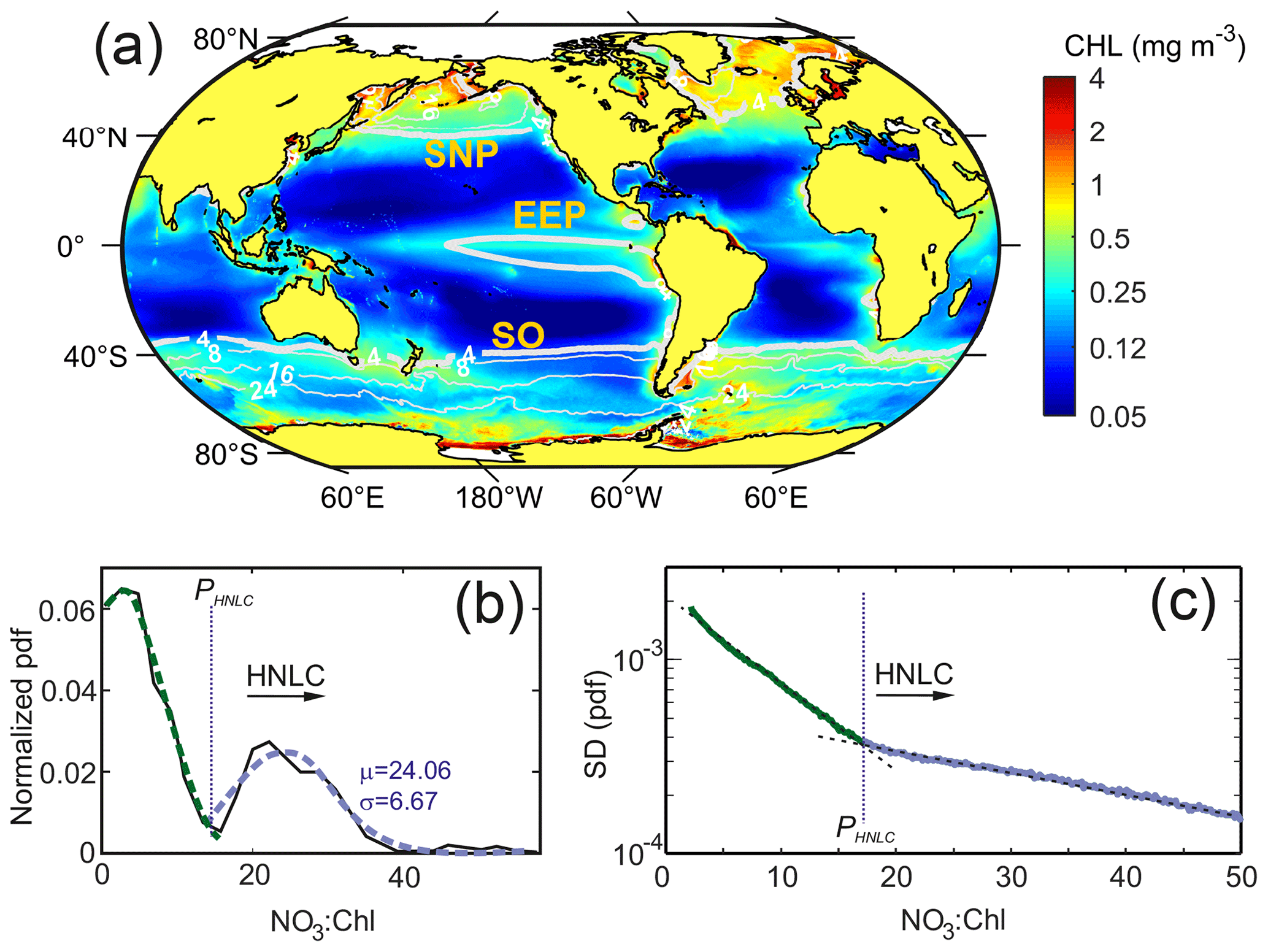
Figure 2 (a) Global mean satellite Chl concentrations (mg m⁻³) for the period 1998–2018 and superimposed mean surface NO₃ contour lines from modeling data. (b) Normalized probability density function of the values of the NO₃ : Chl ratio obtained from the SOM temporal patterns. Green and blue lines show the fit to a normal distribution for the first and second PDF modes, respectively. (c) Standard deviation of the probability density function (PDF) of the NO₃ : Chl (mmol mg⁻¹) monthly ratios obtained for the 20 years analyzed. Note that the y-axis scale is logarithmic. The critical point ratio P_HNLC=17 mmol NO₃ mg Chl⁻¹ delimits HNLC regions from macronutrient-limited regions.

The analysis of the normalized PDF of the NO₃ : Chl extracted from the temporal SOM analysis provides a good discrimination criterion to define HNLC regions (shown in Fig. S2). As shown in Fig. 2b, the normalized PDF of the NO₃ : Chl ratio displays a marked bimodal distribution with the main mode centered at low NO₃ : Chl (∼ 5 mmol mg⁻¹). The second mode, which corresponds to high-nutrient low-chlorophyll regions, is characterized by mean and standard deviation values of μ=24.1 and σ=6.7 mmol mg⁻¹, respectively. A critical NO₃ : Chl ratio bounds the lower limit of this distribution and can be estimated as $\mathit{\mu }-\mathit{\sigma }=\mathrm{17.4}$ mmol mg⁻¹. Consistently, the PDF bulk analysis of its associated standard deviation (SD) function also reveals a clear critical value located where the value of the slope varies (Fig. 2c). Both analyses allow establishing a solid statistical criterion to infer a minimum value of P_HNLC=17 mmol mg⁻¹ for delimiting HNLC regions from other ocean regions. It is worth mentioning that while the PDF of the NO₃ : Chl values obtained from the SOM analysis shows a bimodal mode, the bulk PDF of the raw NO₃ : Chl values (i.e., without performing an SOM analysis) is unimodal.

From the 12 characteristic time patterns of NO₃ : Chl variability obtained in the [4×3] SOM analysis, five display NO₃ : Chl exceeding P_HNLC at all times (not partially) throughout the entire study period (Fig. 3a). These associated subregions (R1 to R5) match the three traditionally reported HNLC regions (Fig. 3b). In these regions surface chlorophyll rarely exceeds 0.8 mg m⁻³, and the mean values range between 0.21 and 0.5 mg m⁻³ (Table 1). The global extent of these five SOM-identified HNLC subregions encompasses 25 % of the ocean, with the SO being by far the broadest region (18 % of the ocean), whereas SNP and EEP respectively occupy some 4 % and 3 % of the ocean. Besides the obvious absence of HNLC regions in the northern and central Atlantic, some latitudinal asymmetries are observed in the distribution of these regions. For example, the SO region extends to lower latitudes than the SNP (i.e., ∼ 40^∘ S), loosely coinciding with the South Antarctic Zone limit (SAZ; Orsi et al., 1995). Likewise, consistent with previous studies of this region (Radenac et al., 2012), the EEP displays a larger extent in the Southern Hemisphere (Fig. 3b).

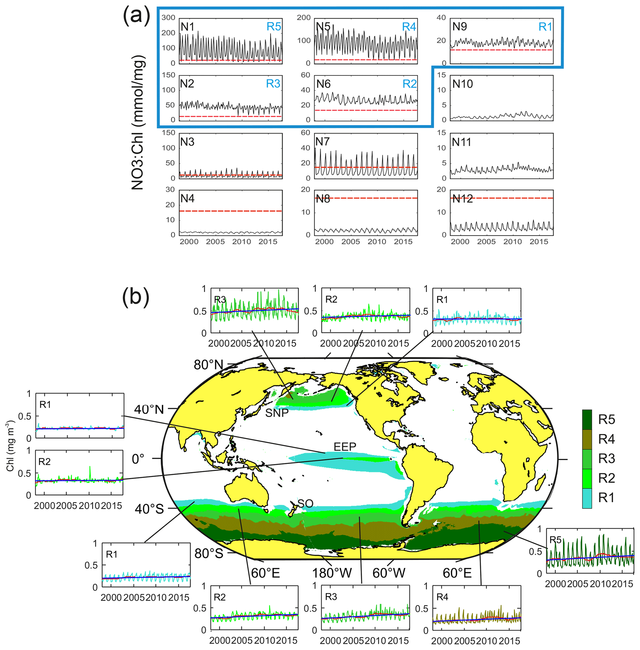
Figure 3 (a) Characteristic temporal variability patterns of NO₃ : Chl ratios (N1–N12) as unveiled by the 4×3 SOM analysis in the time domain. Red dashed lines indicate the P_HNLC value. (b) Coherent regions of HNLC variability (SNP, EEP, and SO) and corresponding subregions (R1 to R5) associated with the SOM temporal patterns exhibiting only NO₃ : Chl values larger than P_HNLC at all times throughout the entire analyzed period (i.e., identified with N9, N6, N2, N5, and N1). Patterns corresponding to a subregion in the Northern and Southern Hemisphere present a similar pattern although seasonally lagged (6-month delay). Insets show the time series of the averaged Chl over the corresponding subregion (complete map of regions of NO₃ : Chl variability and corresponding temporal variability patterns are shown in Fig. S1). The red line represents the 24-month filtered series, and the blue line indicates the trend (values shown in Table 1).

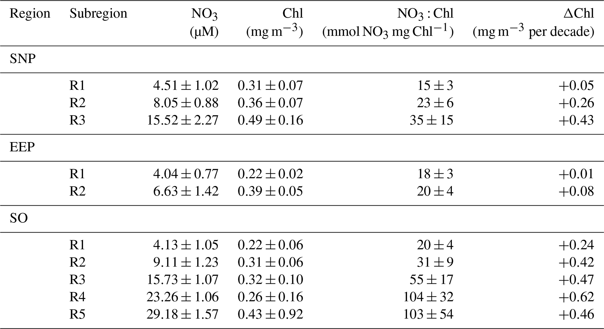
Table 1 Mean ± SD characteristics of each of the SOM-defined HNLC subregions (R1 to R5). NO₃ (mmol m⁻³) and Chl (mg m⁻³) values are respectively from model and satellite data. Decadal chlorophyll trends (ΔChl, mgChl m⁻³ per decade) are calculated from the mean time series of monthly deseasonalized chlorophyll.

The global pattern obtained from the SOM analysis reflects a clear latitudinal zonation, which is mainly due to latitudinal variations in nutrient availability; while the chlorophyll concentration doubles along the latitudinal gradient (R1 to R5), NO₃ increases up to 7-fold (see Table 1). It is noteworthy that nutrient concentrations are generally lower in the SNP (i.e., <17 mmol m⁻³) than in the SO, while Chl is comparatively higher (see Table 1). Indeed, R1 in SNP only achieves the NO₃ : Chl criterion for HNLC regions during some periods. This region exhibits distinctive eastern and western provinces, which are consistent with previous studies describing the western region as more productive and variable (Imai et al., 2002; Harrison et al., 2004).

Major differences among the characteristic NO₃ : Chl patterns in the defined subregions are due not only to variations in mean values, but also to the intensified seasonal variability at higher latitudes. For example, seasonality in Chl is particularly evident in R5 and less so in other polar subregions (Fig. 3b). Conversely, the seasonal component of variability in the EEP is masked by the intense short-term variability.

An interesting feature depicted from the temporal SOM analysis is the positive trend in Chl experienced in the HNLC regions located in polar areas, suggesting an increase in their productivity. Decadal tendencies are in the range of 0.04 to 0.06 mg m⁻³ per decade in the most productive subregions (R2 to R5 in SO and R3 in SNP) but become negligible at the Equator (Table 1). A regional average indicates a Chl increase of 0.6 % yr⁻¹ in the SNP and 1.9 % yr⁻¹ in the SO. Nevertheless, in the case of the SO positive trends are highly influenced by a positive Chl shift occurring at the end of 2010 when mean Chl increased by 24 % (see next section).

3.2 Spatial variability of HNLC regions

The set of nine coherent spatial patterns resulting from the SOM analysis in the space domain and their respective probabilities of occurrence are shown in Fig. 4. The organization of the maps in the figure reveals a hierarchical classification of the maps or spatial patterns. The most differentiated patterns, also displaying the highest probability of occurrence (the probability of finding a pattern similar to the input data), are located in the corners of the neural network, and transitional stages connecting these patterns fill the center. For example, along the top and left side patterns (P1, P2, P3, and P4), generally occurring during winter (see Figs. 4 and 5b), the SNP extends over a larger region compared to P7, P8, and P9, which display a 3 % decrease from the mean extent. Conversely, Fe limitation in the SO, as inferred from high NO₃ : Chl ratios, is markedly enhanced towards the top and right side of the figure (P4, P5, P7, P8, and P9). The extent of the EEP region displays little variation. It should be noted that HNLC spatial extent and NO₃ concentrations are not necessarily coupled since the boundaries also depend on Chl concentration values. In addition, patterns in the proximity of the Antarctic continent are, in some cases, not well-defined during winter due to ice cover in this region.

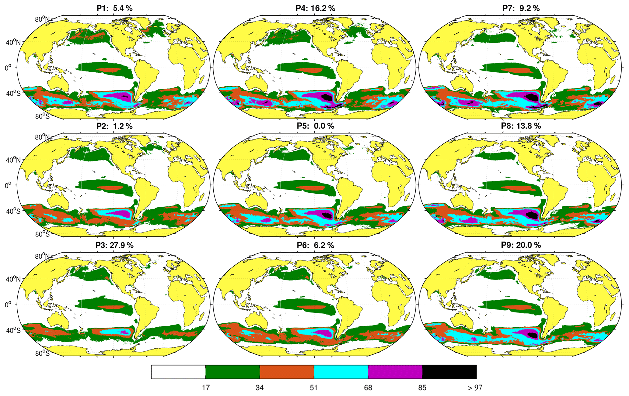
Figure 4 Characteristic spatial patterns (P1 to P9) of HNLC regions as defined by NO₃ : Chl ratios >P_HNLC obtained from monthly data. The value on top of each pattern indicates its probability of occurrence over the 20-year period analyzed. To preserve the topology, the SOM algorithm introduces some patterns with zero probability of occurrence, such as P5. The color bar indicates the different NO₃ : Chl ranges represented.

Figure 5 displays the time series of the BMUs and the monthly frequency of occurrence for each pattern. The main feature observed is the marked seasonality in the patterns shown in Fig. 4. The patterns with the highest probability of occurrence, P3 and P9 (100 % in April and 70 % in July, respectively), represent spring and summer situations in the Northern Hemisphere. P4 and P8 characterize transitions toward these patterns. Other patterns such as P6 and P2 (mostly occurring in winter and summer) are rarer but become more frequent after 2010 (Fig. 5a). As discussed below, this variation in HNLC regional patterns (i.e., P1 is no longer observed) suggests an abrupt and major transition towards more productive HNLC regions (higher Chl is observed).

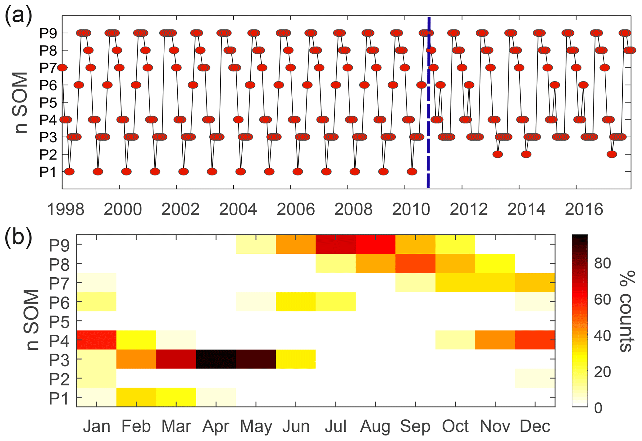
Figure 5 (a) Time evolution of the spatial patterns as defined by the best-matching units (BMUs) for the period of 1998–2018. The blue dashed line indicates the regime shift occurring after 2010. (b) Monthly frequency of occurrence of the spatial patterns identified in Fig. 4.

From the nine spatial patterns shown in Fig. 4, we estimated the seasonal and interannual variation in the extent of the HNLC regions (Fig. 6). Note that this regional partitioning is made on a global scale with global criteria and therefore leads to a large-scale smoothing, which could impact the values of the variation of the areas. However, as this signal smoothing is common to all the areas, this should not have any effect on the regional comparison of the area variation. The magnitude of these variations contrasts remarkably between the equatorial and polar regions. While the extent of the EEP only varies by 8.9 % seasonally, changes in SNP extent can exceed 100 % (Fig. 6). The peak in extent for the SNP corresponds to the boreal spring (63 % of the mean value in April). In the case of the SO, seasonality is mainly driven by changes related to the ice limit at high latitudes. Indeed, the extent of the HNLC region in the austral winter is <20 % of the mean annual extent.

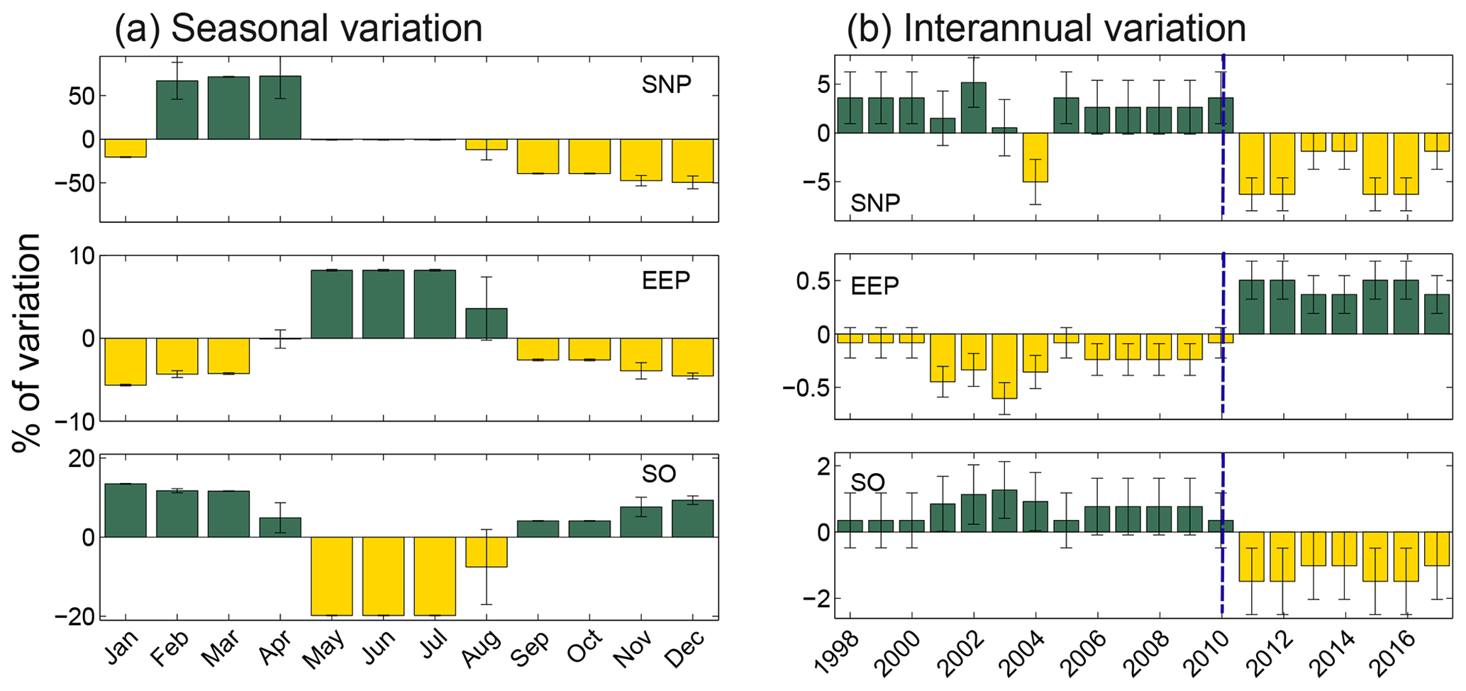
Figure 6 (a) Seasonal and (b) interannual variations in the spatial extent of the three HNLC regions, represented as a percentage of variation from the mean extent of each region. Variations refer to the mean extent of each region. Dark- and light-colored bars indicated positive and negative values, respectively. The blue dashed lines indicate the regime shift occurring after 2010.

A remarkably good inverse correlation ($r=-\mathrm{0.97}$, n=20) is observed between the interannual variations in the extent of EEP and the SO, and a weaker though significant relationship exists between the SNP and the EEP ($r=-\mathrm{0.50}$, n=20). Therefore, as the extent of HNLC in polar regions contracts, the equatorial region expands and vice versa. All three regions exhibit a shift in their annual extent after 2010 (Fig. 6). Both the SNP and the SO decrease after this year (5 % and 2.6 %), whereas the extent of the EEP slightly increases (0.4 %).

3.3 Climate drivers of HNLC region temporal variations

During the period considered here, 1997/1998, 2009/2010, and 2015/2016 showed particularly strong El Niño events, whereas weaker episodes occurred in 2002/2003, 2004/2005, and 2006/2007 (E1, E2, and E3 in Fig. 7a). The 1997/1998 and 2009/2010 El Niño events were followed by fast transitions to La Niña phase (L1 and L2 in Fig. 7a).

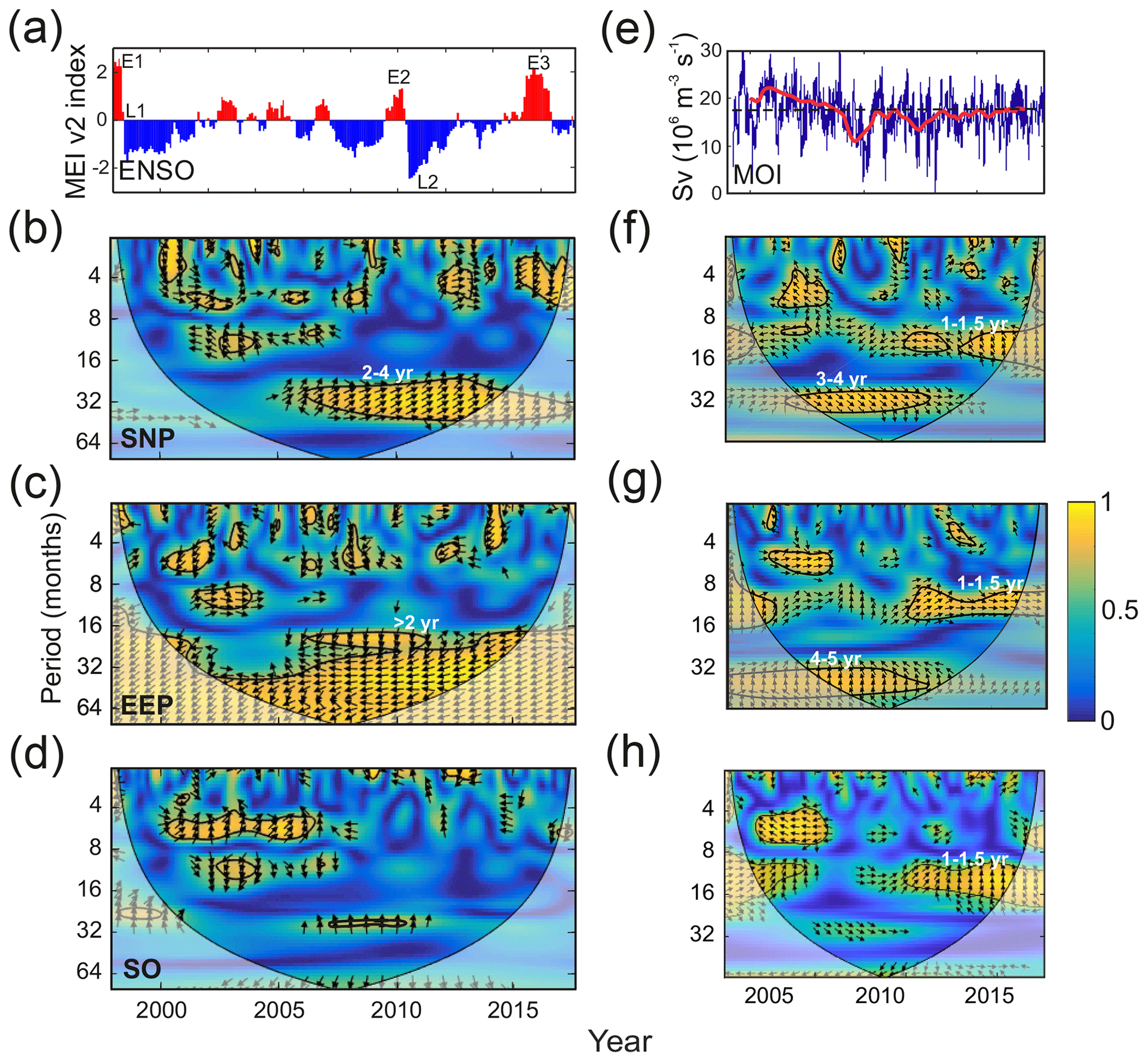
Figure 7 (a) ENSO (MEI v2) index. E1–E3 indicate intense El Niño episodes, and L1 and L2 mark strong La Niña periods. Panels (b), (c), and (d) display the cross-wavelet coherence between NO₃ : Chl ratio and ENSO for each of the HNLC regions. (e) Meridional overturning (AMOC) volume transport for the period 2004–2017 measured at 26.5^∘ N (Smeed et al., 2018). The red line shows that the interannual component is obtained by filtering the data with a 540 d low-pass filter after the removal of the mean seasonal cycle. Panels (f), (g), and (h) display the cross-wavelet coherence between NO₃ : Chl ratio and AMOC for each of the HNLC regions. The thick black contours in the cross-wavelet coherence figures designate the 95 % confidence levels, and the cone of influence where edge effects are not negligible is shown as a lighter shade. The arrows indicate the phase relationship between the signals, with the horizontal component indicating in phase (rightward) or out of phase (leftward) and the vertical component indicating a 90^∘ phase difference lagging (upward) or leading (downward). Period units are months.

The WCA values between NO₃ : Chl ratio in each HNLC region and ENSO are shown in Fig. 7b to d. Generally, small coherence structures are observed at semi-annual periods, in particular in the SO. However, the main coherence pattern corresponds to a band extending in the 2 to 4 years in the SNP and >2 years in the EEP. This coherence between NO₃ : Chl and ENSO in the 2–4-year period is particularly clear after 2005 (Fig. 7b). In the EEP, the coherence between the two series expands to periods >4 years, but, unlike in the SNP region where the NO₃ : Chl ratio is in phase with the ENSO signal, the signals are strongly anticorrelated in this case (antiphase: relative phase of 180^∘ between the two signals).

Figure 7e shows the MOC transport index (hereafter MOI) measured at 26.5^∘ N (Smeed et al., 2019). MOI displays intense interannual variability; however, a clear long-term variation is observed. Transport exceeds 17 Sv until 2009, but it weakens during 2010, stabilizing thereafter. As shown in Fig. 7f to h coherence with NO₃ : Chl ratios is strongest at interannual timescales (1–1.5 years) when MOC is debilitated.

4 Discussion

4.1 Global characterization of HNLC regions

In the present study, we have addressed the extent of the HNLC regions, their long-term variability, and the potential drivers of these variations. Despite the relevance of precise characterization of the extent of this biome for the understanding of physical ocean processes (i.e., upwelling) and the estimation of the amount of carbon drawn into the ocean by phytoplankton, objectively determining the boundaries of HNLC regions has remained elusive as it requires coherent information on both nutrients and Chl. We demonstrate that a statistical approach, based on a threshold in the distribution of the global NO₃ : Chl ratios, can robustly delineate these regions (P_HNLC). This is also evidenced in Table 1 where the characteristics of each cluster obtained with SOM analysis are remarkably constant (i.e., low SD).

As in preceding studies (e.g., Moore et al., 2013), we assume that excess NO₃ in surface oceanic areas is indicative of Fe limitation. This avoids relying on the scarce information available on Fe stress or more complex ecosystem modeling approaches. Inference of phytoplankton Fe stress from satellite ocean color data has been attempted but it is a methodology that still presents large uncertainties (Browning et al., 2014). Furthermore, while bioavailable Fe is known to be the primary limiting factor in this biome, the establishment of HNLC conditions is influenced by various other factors such as light availability, grazing pressure, rate of Fe remineralization, and community structure, highlighting the diverse interrelations among these factors. Despite these drawbacks, the method developed herein provides results consistent with previous descriptions of the large-scale spatial patterns of HNLC regions, mostly based on NO₃ fields (i.e., Archer and Johnson, 2000; Ono et al., 2008; Fu and Wang, 2022). Also, the proposed method for biome definition may introduce a bias in that the resulting spatial fields are smoother compared to those based on Fe limitation, which is due to the greater variability of Fe concentrations compared to NO₃ fields.

The P_HNLC obtained from the PDF distribution of the NO₃ : Chl ratios represents a statistical threshold that integrates complex biological processes, including competition for resources, grazing, changes in species composition, nutrient uptake rates, and Fe-regulated algal photochemistry. Unlike Redfield or C : Chl ratios, which respond to physiological factors within phytoplankton cells, P_HNLC can be considered an environmental indicator of changes in the structure and functioning of marine phytoplankton.

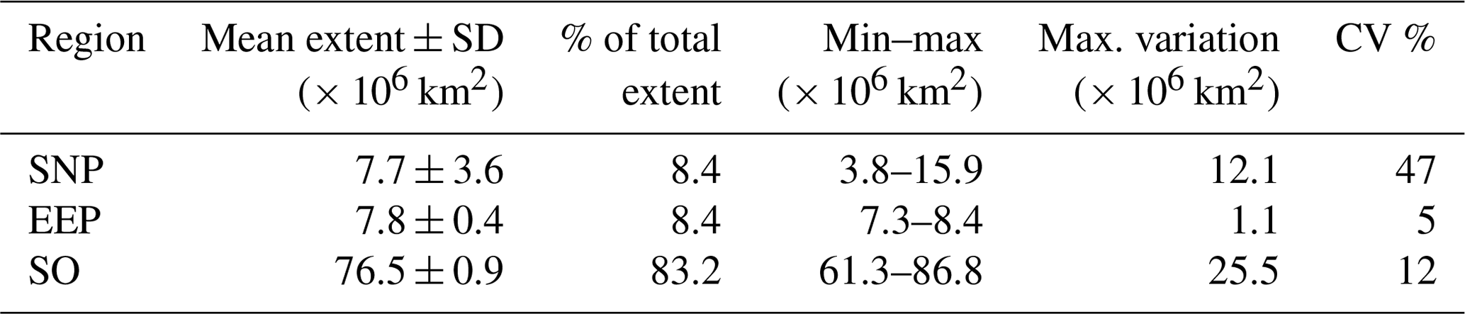
According to our analysis, some 25 % of the ocean (18 % of the Earth's surface) corresponds to unproductive HNLC waters. With 83 % of the global HNLC biome extent, the SO is the largest region and it is the only one presenting clear latitudinal variation in the characteristic Chl patterns (Table 2 and Fig. 3). This is consistent with available descriptions of the physical and chemical properties of the SO, which tend to be across latitude due to the meridional structure of the MOC and because of the rapid zonal redistribution imposed by circumpolar currents (Orsi et al., 1995). The SNP and the EEP each constitute ∼ 8 % of the total HNLC. However, while the EEP remains relatively stable (cv = 5; Table 2), the SNP can change up to 2-fold (Fig. 4 and Table  2).

Table 2 Basic statistics of the annual extent of each of the SOM-defined HNLC subregions during the analyzed period (1998–2017). Maximum variation (max. variation) is calculated as the difference between the maximum and the minimum extent.

Our analysis reveals marked decadal tendencies in Chl in the most productive subregions, ranging between 0.04 and 0.06 mgChl m⁻³ per decade, and negligible trends in the EEP (Table 1). Positive Chl trends at high latitudes and no significant tendencies at the Equator at the 95 % interval have been previously reported by Hammond et al. (2017). Indeed, climate change projections for the 21st century predict declines in global marine net primary production but increasing Southern Ocean productivity (Hauck et al., 2015; Moore et al., 2018). Nevertheless, it is noteworthy that our analysis shows that trends in some regions of the Southern Hemisphere are influenced by a Chl shift occurring in 2009–2010 (particularly R4 and R5). The possible source of this shift in phytoplankton biomass is more extensively discussed below. However, it is unlikely to be related to satellite data merging. SeaWiFS ended operations in 2010 and the MERIS sensor ceased in April 2012; however, a decrease in biomass would be expected from these changes (Garnesson et al., 2019).

4.2 Spatial variability of HNLC regions

SOM analysis allowed the characterization of the seasonal and interannual variability of HNLC regions (Figs. 5 and 6). The SO and the SNP are regions of seasonal extremes in productivity as a consequence of the large fluctuations in the environment that they experience. Important seasonal variability is observed in the SO, which is attributed to light limitation during winter and to variations in iron stocks occurring in surface waters (Tagliabue et al., 2014). Therefore, while presenting HNLC characteristics for most of the year, the SO exhibits distinct Chl variability patterns that are well-captured in the SOM regionalization and the characteristic patterns of each subregion. In the case of the SO, the changes in the extent are reduced (20 % from mean values), which we attribute to the large-scale nature of the physical processes regulating the productivity of this region. Mid-depth and deep-ocean waters communicate with the ocean surface after following a circuit route driven by ocean overturning circulation (Lumpkin and Speer, 2007). As reported by Smeed et al. (2018), the variability of the MOC flow system has an important decadal component associated with thermohaline forcing. This long-term component of variability could dominate over higher-frequency variability, but the length of the observational record of the AMOC is still insufficient to resolve variations at this scale.

Variability patterns in the SNP are attributed to both marked seasonality in the local forcings and fluctuations in the regional circulation patterns. Nishioka et al. (2021) discuss the sources of phytoplankton variability in this region in detail, distinguishing three cases of biological response to Fe in this region. The annual bloom in open waters would be controlled by the sedimentary Fe supplied from the continental marginal regions and circulated laterally through the intermediate layer (e.g., Lam et al., 2006; Cummins and Freeland, 2007; Takeda, 2011). These nutrients are upwelled to the surface by several mixing processes (winter mixing and eddy diffusive mixing), including interactions of tidal currents with the rough topography (Nishioka et al., 2007, 2020). Massive spring phytoplankton blooms that occur around the coastal boundary current would be the result of the large amounts of Fe originating from coastal shelf areas (Cullen et al., 2009). Finally, intense, sporadic, and patchy phytoplankton production is occasionally observed in both spring and summer in response to the atmospheric dust Fe supply.

Marked differences in variability are observed between the subpolar regions and the EEP, where seasonality is weak. Nevertheless, it should be noted that the EEP is a peculiar region that integrates subregions with 6-month out-phased seasonal variations (north and south of the Equator). On average, the southern equatorial region contributes more (62 % of the total extent) to the mean extent of the EEP, whereas the northern subregion determines most of the observed variability (Fig. S3).

At interannual scales, variations in the extent of HNLC regions are more modest (up to 5 %; Fig. 6) but all three regions are notably correlated, suggesting that their interannual variations are driven by global-scale processes. In particular, the SO and the EEP are highly correlated (r=0.97). A coupling between Southern Ocean productivity and equatorial productivity was suggested by Dugdale et al. (2002) based on the observed nutrient ratios. They proposed that both regions were connected, out of phase, by the meridian Sub-Arctic Mode Water. Nevertheless, the seaways in the Pacific circulation pathways are complex, and determining the overturning signature is challenging. Some studies have suggested that temperature anomalies subducted into the pycnocline at subtropical latitudes may not reach the Equator with any appreciable amplitude (Schneider et al., 1999). However, mass water balances in the equatorial Pacific reveal that the strength of the equatorial upwelling is related to variations in the Pacific overturning (PMOC; McPhaden and Zhang, 2002), and therefore, an influence on EEP extent could be presumed. Nevertheless, it should be remembered that the extent of the HNLC regions is not necessarily solely dictated by upwelling intensity; it is also defined by the interaction with adjacent circulation patterns (i.e., the subtropical gyres in this case).

The pathways of PMOC in the North Pacific are structured in a multicell configuration. The SNP does not ventilate the deep ocean at significant rates, and the PMOC cell at this latitude rather corresponds to an independently functioning intermediate water cell (Warren, 1983). PMOC in this region is reportedly weak (1–4 Sv) and extends no further than 50^∘ N (Ishizaki, 1994; Yaremchuk et al., 2001). However, there is evidence showing the response of the SNP to changes in PMOC (Burls et al., 2017; Holzer et al., 2021). For example, it has been observed in TOPEX altimeter data that meridional overturning transport influences the basin-scale baroclinic circulation in the SNP. This would explain the lower, yet significant, correlation with the variations exhibited by SO and EEP at interannual scales (Fig. 6). Indeed, the shift observed in 2009–2010 is common to all three regions (although with a different sign).

The causes of the drastic 2009–2010 variation in the extent of HNLC regions are uncertain. Several ocean-scale changes have been reported in the period 2009–2011. For example, rapid warming, salinification, and a concurrent dissolved oxygen decline were observed for the Bermuda Atlantic Time-series Study (BATS) during the 2010s (Bates and Johnson, 2020). There is also evidence indicating that a decadal intensification of Pacific trade winds weakened in 2011 (Bordbar et al., 2019). Trade wind intensity variability in the equatorial Pacific region is associated with sea surface temperature (SST) anomalies, weakening of the equatorial divergence, and changes in upper-ocean thermal structure (England et al., 2014; Bordbar et al., 2017). The relationship between the equatorial wind intensity and the equatorial undercurrent strength is well-established (McPhaden, 1993). These atmospheric changes, affecting the upwelling of Fe in the EEP (and indirectly to other oceanic regions), agree with the hypothesis of Winckler et al. (2016), suggesting that ocean dynamics, not dust deposition, control the equatorial Pacific productivity. In the EEP the period of strongest seasonal upwelling is in the boreal summer (e.g., Philander and Chao, 1991), which is associated with an expansion of the HNLC in Fig. 6a. We also observe an expansion of the extent of the HNLC region in the EEP after 2021 (Fig. 6). Changes in these forcings could explain variations in the seasonal variability, but the long-term changes in HNLC extent would require more a permanent variation in the stoichiometric equilibria or in the functioning of the marine food webs.

4.3 Drivers of HNLC region variability

ENSO is the primary source of the interannual variability in the EEP, and its occurrence is related to the decline in nutrient supply. For example, the deepening of the thermocline during ENSO is associated with the depression of the Equatorial Undercurrent (EUC) that transports Fe across the basin from the western Pacific (Gordon et al., 1997), also reducing nutrient supply and phytoplankton productivity (Chavez et al., 1999; Strutton and Chavez, 2000). Sub-decadal fluctuations in Chl in the EEP region displaying a good correlation with the ENSO index have been reported before (Oliver and Irwin, 2008; Boyce et al., 2010). By contrast, the SO only shows weak evidence of this relationship, which suggests that ENSO is not a major forcing driving the variability of NO₃ : Chl in this region. This is consistent with reports from Ayers and Strutton (2013), who did not find a significant relationship between nutrients in this region and ENSO.

It can be argued that differences in the response to ENSO are due to the different nature of the forcings driving nutrient supply in each region. While the EEP and the SNP seem to respond to ENSO-related changes, NO₃ : Chl ratios in the SO are more stable and respond to annual and semi-annual variations. The coupling between the EEP and the SNP dynamics has been reported before. Qiu (2002) observed progressive shoaling of the Alaska gyre caused by a strengthening of the cyclonic circulation. The interannual variability of this gyre was connected to ENSO-related sea surface height anomalies originating in the tropics. Several large-scale climate pattern indexes are invoked to explain physical and biological fluctuations in the SNP. For example, Di Lorenzo et al. (2008) defined the North Pacific Gyre Oscillation (NPGO), which explains strongly correlated fluctuations of salinity, nutrients, and chlorophyll related to the circulation in the North Pacific Gyre. It is beyond the scope of the present work to assess the relationships of all these indexes with the variability in the extent of HNLC regions. Nevertheless, the proposed climate indexes for the Pacific present a strong relationship among them, which highlights the strong dynamical linkages between tropical and extratropical modes of climate variability in the Pacific basin and the important role played by ENSO (Di Lorenzo et al., 2013).

The interpretation of the influence of MOC on global ocean productivity is more challenging. A stronger MOC should result in faster upwelling of macronutrients and Fe at high latitudes as well as in increased Ekman transport of nutrients equatorward and subsequent subduction (Ayers and Strutton, 2013). Consequently, a weakened MOC should plausibly favor Fe recycling rates, as reported by Rafter et al. (2017).

At high latitudes, the weakening of the AMOC is coherent with a decrease in the extent of the SNP and the SO (Fig. 5). This anomaly, starting in 2009–2010, is a global feature also reflected in the Intertropical Convergence Zone (ITCZ) time series (see Green et al., 2017; Ibánhez et al., 2017), suggesting a strong atmosphere–ocean coupling with an impact on ocean productivity. It is not clear how a reduced flow would favor the increase in biomass at high latitudes. It has been proposed that a reduced AMOC from increased precipitation and melting sea ice could contribute to reduced vertical mixing, which may increase productivity in polar regions (Riebesell et al., 2009). Other studies (Martínez-Garcia et al., 2009) showed a relationship between AMOC and Chl variations, mainly due to the interaction of the main pycnocline and the upper-ocean seasonal mixed layer. In addition, some paleoclimatic studies have demonstrated that AMOC weakening can increase the productivity north of the Polar Front, but only if an increase in the atmospheric soluble Fe flux occurs (Muglia et al., 2018). Paleoceanographical records showing a strong correlation between proxies of aeolian Fe flux and productivity have been reported in this region (Kumar et al., 1995; Martínez-Garcia et al., 2009) but, in present times, dust deposition in this area is notably different (i.e., McConnell et al., 2007), and this effect is unlikely to be important at the timescales considered here. Complex ecosystem processes including competition for Fe with bacteria, Fe remineralization rates, and organic complexation processes could determine the phytoplankton response under future scenarios. Further, biomass build-up is driven not only by nutrient availability. Changes in biomass can be produced by variations in the thermocline depth, affecting the vertical distribution of phytoplankton. Nevertheless, variations in phytoplankton composition, physiological adjustments in cellular pigmentation, and grazing could also modulate Chl variability. Indeed, the prevailing food web structure may play an important role in Fe fertilization (Schmidt et al., 2016). At larger scales, there are still unresolved questions about the couplings occurring at different temporal scales. For example, MOC variations are known to interact with ENSO, influencing its amplitude and variance (Dong et al., 2006; Dong and Sutton, 2007; Timmermann et al., 2007).

5 Conclusions

Variations in the boundaries of the HNLC regions can provide an integrative view of how climate-scale ocean variations influence ocean productivity. We established a statistical criterion to identify HNLC regions from global Chl and NO₃ data that sets the basis for systematic analyses of HNLC regions and their response to climate variations.

Our results suggest that while local-scale processes can determine certain aspects of the productivity of HNLC regions, their long-term patterns are strongly influenced by variations in global atmospheric and oceanic circulation. We observed significant interannual variations in the extent of HNLC regions (up to 5 % in Fig. 6), which are associated with anomalies in global ocean circulation patterns (i.e., Fig. 7e). Accordingly, our findings suggest a scenario in which HNLC regions are vulnerable to interbasin teleconnections rather than local forcings. These general patterns may be modulated by feedback between different forcing mechanisms. Furthermore, our analysis reveals a shift in phytoplankton biomass and HNLC variation patterns occurring at the end of 2010, which evidences the occurrence of fast transitions in ocean biogeochemistry. The underlying drivers of these regime shifts and the resulting biological responses to these ocean-scale changes require further investigation since they are a fundamental aspect of long-term variations in marine ecosystem functioning.

Finally, the present study highlights the importance of maintaining long and coherent datasets beyond satellite-borne information to be able to disentangle the different components of variability, particularly at long timescales, and to evaluate the impact of climate change on marine ecosystems. Most of the geochemical information at this scale (i.e., nutrient and Fe fields) will probably require further global sampling programs and refined modeling.