the Creative Commons Attribution 4.0 License.
the Creative Commons Attribution 4.0 License.
 | 03 Mar 2022
Using machine learning and beach cleanup data to explain litter quantities along the Dutch North Sea coast
Mikael L. A. Kaandorp
Stefanie L. Ypma
Marijke Boonstra
Henk A. Dijkstra
Erik van Sebille
Coastlines potentially harbor a large part of litter entering the oceans, such as plastic waste. The relative importance of the physical processes that influence the beaching of litter is still relatively unknown. Here, we investigate the beaching of litter by analyzing a data set of litter gathered along the Dutch North Sea coast during extensive beach cleanup efforts between the years 2014 and 2019. This data set is unique in the sense that data are gathered consistently over various years by many volunteers (a total of 14 000) on beaches that are quite similar in substrate (sandy). This makes the data set valuable to identify which environmental variables play an important role in the beaching process and to explore the variability of beach litter concentrations. We investigate this by fitting a random forest machine learning regression model to the observed litter concentrations. We find that tides play an especially important role, where an increasing tidal variability and tidal height leads to less litter found on beaches. Relatively straight and exposed coastlines appear to accumulate more litter. The regression model indicates that transport of litter through the marine environment is also important in explaining beach litter variability. By understanding which processes cause the accumulation of litter on the coast, recommendations can be given for more effective removal of litter from the marine environment, such as organizing beach cleanups during low tides at exposed coastlines. We estimate that 16 500–31 200 kg (95 % confidence interval) of litter is located along the 365 km of Dutch North Sea coastline.
- Article
(6389 KB) - Full-text XML
- BibTeX
- EndNote


The accelerated release of mismanaged plastic waste into the global ocean gives rise to the need for effective cleanup strategies (Ogunola et al., 2018). In order to minimize the negative impact of plastic pollution on the environment, cleanup strategies need to be optimized to target the most impacted areas while limiting the economic cost (Haarr et al., 2019; Newman et al., 2015). Recent studies indicate that plastics remain trapped in coastal zones (Koelmans et al., 2017; Lebreton et al., 2019; Kaandorp et al., 2021a; Morales-Caselles et al., 2021), with at least 77 % of buoyant marine plastic debris beaching or floating in coastal waters (Onink et al., 2021). Therefore, beach cleanups have the potential to be a highly effective mitigation measure.
In addition, the plastic concentrations found on beaches are generally higher compared to other environmental compartments, such as the surface water or the seafloor (Morales-Caselles et al., 2021), making beaches favorable locations for cleanup activities. Furthermore, by limiting the resuspension of plastic items by removal, the overall plastic concentration on the beach decreases over time and the formation of microplastic is reduced (Andrady, 2011; Haarr et al., 2020; Lebreton et al., 2019). At the same time, as cleanup activities generally involve a large number of volunteers, awareness of the plastic pollution problem increases, leading to a reduction of plastic waste in the local environment (Kordella et al., 2013).
Although the benefits of beach cleanups are well known, the location and timing of these activities are often not optimized. Haarr et al. (2019) identified accumulation zones of beached plastic using the shoreline curvature and gradient in Lofoten, Norway, and showed that high-accumulation areas are often missed by cleanup actions. Other coastal properties like substrate and backshore type have been found to influence debris quantities as well (Hardesty et al., 2017; Brennan et al., 2018), with more litter accumulating in areas with increased backshore vegetation. Additionally, physical processes play an important role in the beaching of plastics and should be considered when selecting effective sites for beach cleanups.
However, the relative importance of the various physical processes involved and how these can be parameterized so far remains unknown (van Sebille et al., 2020; Pawlowicz, 2020). Studies have addressed the importance of the landward wind direction for debris accumulation rates (Eriksson et al., 2013; Critchell et al., 2015; Hengstmann et al., 2017; Moy et al., 2018), the landward ocean circulation direction (Thepwilai et al., 2021), and the role of tides (Eriksson et al., 2013; Pawlowicz, 2020) and waves (Williams and Tudor, 2001). The spatial and temporal variability of the sources, e.g., rivers, population density, and the fishing industry, also play an important role for the accumulation of plastic on beaches (Rech et al., 2014; Critchell and Lambrechts, 2016).
In addition to the study by Haarr et al. (2019), there are several other studies that assess the prediction or monitoring of beached plastic items using machine learning methods. These algorithms can be useful in discovering complex relations between environmental variables and litter concentrations. In Granado et al. (2019), a marine litter forecasting model was made using Bayesian networks, involving various variables like wave height and period, wind velocity and direction, precipitation, and river flow. Neural networks have been used to quantify litter categories in Balas et al. (2004) and Schulz and Matthies (2014), and deep learning methods have been used to automatically identify debris on beaches (Song et al., 2021).
In order to make data-driven methods work, relatively large and consistent data sets are necessary, but most observational data sets are sparse. Beach cleanups and citizen science initiatives can potentially provide valuable information for scientific studies on marine pollution (Zettler et al., 2017), as these data are based on a considerable amount of person hours. Examples of citizen science data used in marine pollution research can be seen in the work of Hidalgo-Ruz and Thiel (2013), where schoolchildren in Chile documented the distribution and abundance of plastic debris on beaches, and Ribic et al. (2010, 2012), where amounts of marine debris were measured by volunteer teams on beaches in the Pacific and Atlantic.
Here, we will build upon past data-driven studies by using an unprecedented data set obtained from beach cleanup efforts organized along the Dutch North Sea coast between 2014 and 2019. The number of participants (about 14 000), person hours (about 84 000 h), the length of beach sampled (about 1400 km), and the fact that all beaches sampled were similar in substrate (sandy) make this data set unique and very appropriate to apply data-driven methods. Furthermore, a large set of explanatory variables will be created based on environmental conditions and modeled transport of marine litter. We will fit a random forest regression model to the observed litter concentrations as a function of these explanatory variables and investigate which ones are important to explain the variability in beach litter. This allows us to investigate which variables are important predictors for the amount of litter present on beaches to get a better understanding of marine pollution and to increase the efficacy of beach cleanups by creating a predictive model that could aid future cleanup efforts.
Since 2013 the North Sea Foundation, a Dutch environmental non-governmental organization (NGO) advocating the protection and sustainable use of the North Sea marine ecosystem, has organized the national Boskalis Beach Cleanup Tour. During this tour, every year in August the entire Dutch North Sea coast is cleaned up by volunteers. It is the largest cleanup campaign in The Netherlands. The tour is divided into stages along the North Sea coast. The length of each stage is between 8–10 km. The midway points of all stages are plotted in Fig. 1 using the black crosses.
During the first three editions (2013–2015), the tour was organized over a period of a month, with one stage per day. From 2016 on, the tour took 15 d, with simultaneous cleaning of two stages per day. One cleanup team started on the Wadden Island Schiermonnikoog (the easternmost cross in Fig. 1), the other team started in the southwestern province Zeeland in Cadzand (the westernmost cross in Fig. 1). On day 15, both teams met halfway in Zandvoort (≈4.5∘ E). The cleanups started around 10:00 LT (local time) and ended around 16:00 LT, with total cleanup times taking between 4 and 6 h for each stage. The volunteers were guided by cleanup teams of the North Sea Foundation, which consist of professional employees of the North Sea Foundation and trained volunteers.
At each stage, all litter present on the beach was collected in plastic bags and weighed. The weighing of the collected litter was done using analogue and/or digital scales (during the stage or at the end of the stage) and carried out by one of the members of the cleanup team. Most of the litter found was plastic (estimated percentage between 80 %–90 % in terms of numbers). The years over which weights of collected litter are available for each stage are plotted in Fig. 1 using the colored squares. For most stages, weights are available for all years, in some cases stages were added in later years. Figures with the observed amount of litter per location per year are presented in Figs. A1 and A2.
To get an impression of the mean environmental conditions along the Dutch North Sea coast, the mean surface currents are plotted in Fig. 1 using the arrows (Global Monitoring and Forecasting Center, 2021), and the mean wind speed and direction are plotted using the wind rose (Hersbach et al., 2020), all averaged over August between 2014 and 2019. The wind predominantly comes from the southwest. Generally, the currents move from southwest to northeast along the North Sea coast. The effect of freshwater influxes from rivers is visible around the southern province of Zeeland (<52∘ N). The effect of this freshwater influx can be observed over considerable distances along the Dutch coast, for example in the form of freshwater lenses traveling downstream (De Ruijter et al., 1997; Rijnsburger et al., 2021). Ricker and Stanev (2020) found that locations with high-salinity gradients due to a freshwater influx can act as a barrier for neutrally buoyant particles, possibly causing accumulation of litter along these fronts. Finally, tidal currents move along the coast to the northeast during flood tide and southwest during ebb tide (not plotted in the Fig. 1).
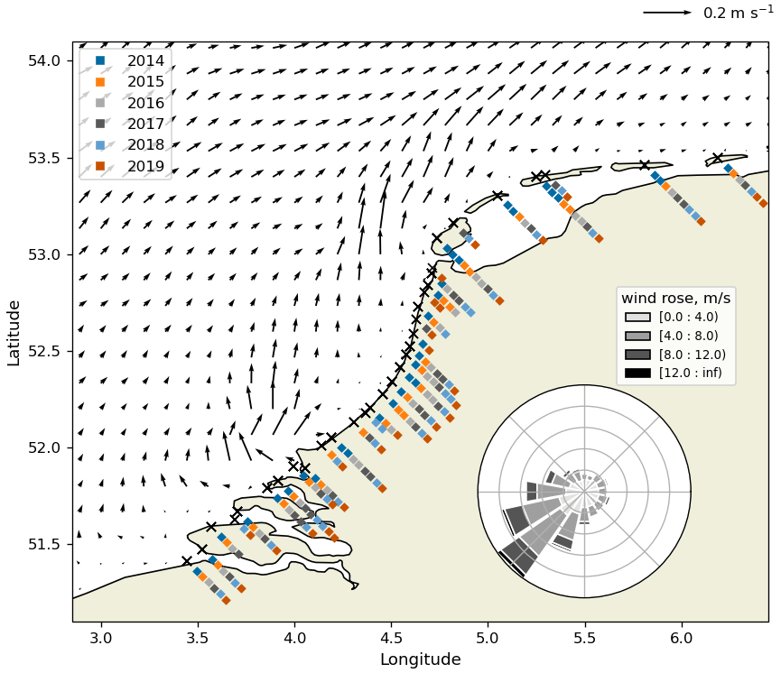
Figure 1Locations of the midway points for each cleanup tour stage (black crosses) and dates showing for which year data are available (the colored squares). For stages with multiple data points per year, different stretches of beach were cleaned (e.g., once on the northern side and once on the southern side). Also plotted are the mean surface currents (arrows) (Global Monitoring and Forecasting Center, 2021) and the wind rose (Hersbach et al., 2020) calculated for August for the years 2014–2019.
3.1 Data preprocessing
Different sources of marine litter exist, such as mismanagement of waste near the coast, input from rivers, or fishing gear which is lost at sea. The litter is then transported through the environment and can eventually end up on beaches, influenced by various factors such as ocean currents and winds. However, how all of these variables combined influence the beaching of litter is unknown. A regression model is used here to relate various environmental variables to the observed litter concentrations. We will assess whether it is possible to use the regression model to make predictions about the amount of beached litter and, if so, which environmental variables are important predictors to take into account.
For the environmental variables, three classes of data are used. First of all, hydrodynamic data (ocean currents, ocean surface waves, tides) and wind data are used (Sect. 3.1.1). Furthermore, we use Lagrangian simulation data, capturing transport of virtual particles representing floating litter. These simulations are used to estimate fluxes of litter onto beaches (Sect. 3.1.2). Finally, we use data of the coastal geometry and orientation (Sect. 3.1.3). Environmental variables are calculated for various lead times and distances from the measurement locations (expressed as radii around the stage midway points). These variables are then fed into a random forest algorithm to make the regression model.
3.1.1 Hydrodynamic and wind data
Numerical model data are used to specify the state of the sea and wind around the beach cleanup locations, as these factors have been found to likely play a role in the accumulation of beach litter (Eriksson et al., 2013; Thepwilai et al., 2021; Williams and Tudor, 2001). Reanalysis data are used where historical observational data have been assimilated in numerical models.
Information about ocean surface currents (Ucurr.), salinity (S), Stokes drift (UStokes), and significant wave height (Hs) are derived from EU Copernicus Marine Environmental Monitoring Service Information data. High-frequency tidal forcing has been used to produce the ocean current data, but output is only provided daily. To capture the effects of tides on a high temporal resolution, FES2014 data are used. Tidal currents (Utides) and heights (htide) are calculated, taking the M2, S2, K1, and O1 constituents into account (Sterl et al., 2020), as well as the M4 and M6 components, which have been shown to play an important role in transport of suspended particles in the North Sea (Gräwe et al., 2014). The wind velocity field at 10 m (Uwind) is taken from ERA5 reanalysis data. ERA5 data are used for the atmospheric forcing in the European Northwest Shelf reanalysis product from which the surface current data are obtained, making these data sets consistent. Further details on the temporal and spatial resolution and assimilated data are given in Table 1.
Global Monitoring and Forecasting Center (2021)Global Monitoring and Forecasting Center (2020)Lyard et al. (2021)Hersbach et al. (2020)Table 1An overview of the numerical hydrodynamic and wind data used to derive the variables for the regression analysis. The data set name, temporal and spatial resolution, data used to assimilated the numerical models, and corresponding references are presented.
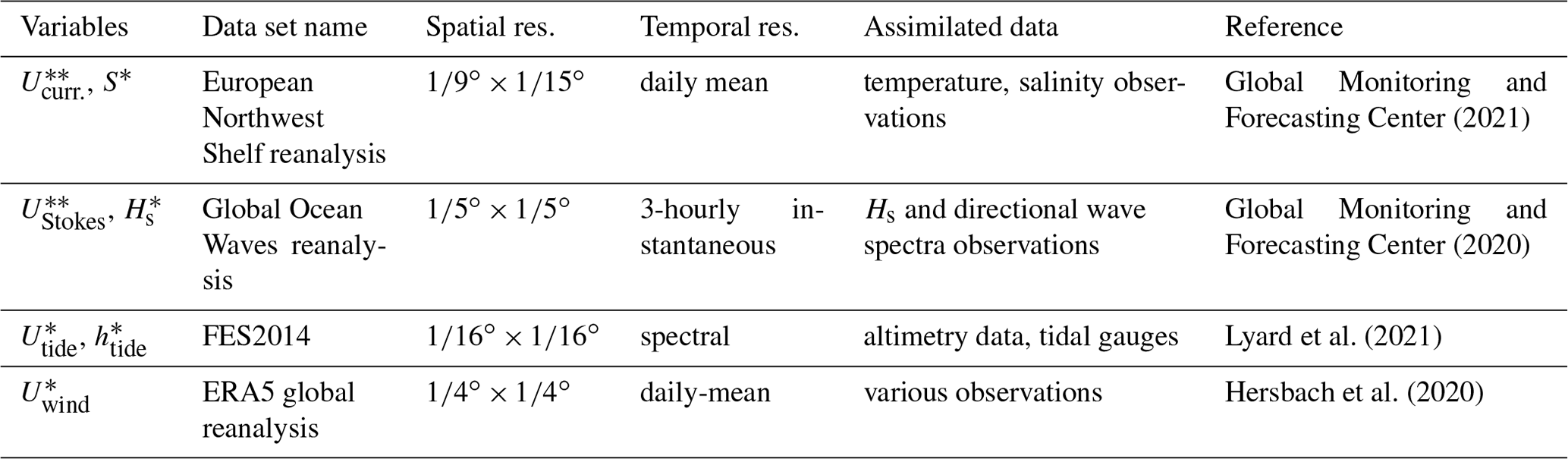
* Data are used from July to September for the years 2014 to 2019. Data are used for all months from January 2011 up to September 2019, as these are also used for the Lagrangian model simulations.
3.1.2 Lagrangian model setup
While data on the sea state and wind might explain the litter accumulating on beaches to some extent, it misses information on possible sources of litter and how this litter is transported through the marine environment. We therefore include estimates of beached litter fluxes in our analysis based on Lagrangian particle simulations.
Using the OceanParcels Lagrangian ocean analysis framework (Delandmeter and van Sebille, 2019), we model the trajectories of virtual buoyant particles at the sea surface using a Runge–Kutta 4 integration scheme. These virtual particles represent floating litter such as plastics. For the trajectories we consider a domain between 40–65∘ N and 20∘ W–13∘ E; see Fig. 2. We simulate a total of about 380 000 trajectories over the years 2011–2019. When particles move out of the specified domain they are removed, which mainly happens after particles move northward along the Norwegian coast. The ocean surface currents and Stokes drift from the hydrodynamic data are used to move the virtual particles around. We do not add additional tidal forcing to the Lagrangian model (Sterl et al., 2020) since the net effect of tides is already included in the ocean surface current data set (Global Monitoring and Forecasting Center, 2021). It is assumed that particles move just below the surface water and do not experience a direct wind drag (Lebreton et al., 2018; Macias et al., 2019; Kaandorp et al., 2020). Effects of subgrid-scale phenomena are parameterized using a zeroth-order Markov model (van Sebille et al., 2018). The tracer diffusivity is set to a constant value of 10 m2 s−1, appropriate for the given mesh size (Neumann et al., 2014).
We use the same approach as in Kaandorp et al. (2020) to define sources of marine plastic litter. Particles are released daily at river mouths, proportional to the estimated monthly riverine outflow of plastic waste based on the model by Lebreton et al. (2017). These sources are plotted using green circles in Fig. 2. Particles are released daily in the sea, proportional to the amount of fishing hours based on Kroodsma et al. (2018), shown in blue in Fig. 2. These data are dependent on fishing vessel transponders, which are not equally present over the years. We therefore release a constant input of virtual particles from this source each day. Finally, there is a constant daily release of particles along coastlines proportional to the amount of estimated land-based mismanaged plastic waste within a radius of 50 km from the coastline (Jambeck et al., 2015; SEDAC et al., 2005). These sources are plotted in red in Fig. 2.
A beaching timescale τbeach parameterizes how quickly litter moves from the sea onto the beach when residing near the coast (Kaandorp et al., 2020). Here, the probability of beaching Pbeach is given by
where tcoast is the time that particles spend in the model ocean cell adjacent to the coast. Various values for τbeach are tested here, from τbeach=25 d estimated for plastic particles and τbeach=75 d estimated for drifter buoys in Kaandorp et al. (2020), to a more conservative value of τbeach=150 d. While in reality τbeach might vary significantly both in space and time, it is unknown how this can be best parameterized (Onink et al., 2021). We use the Lagrangian model simulations to capture the large-scale transport of litter and allow the regression model to pick the most appropriate value for τbeach later on. Only direct pathways of litter through the surface water are considered here and resuspension of litter from beaches (Onink et al., 2021) is ignored. Particles are tracked until they have lost more than 99 % of their initial mass in the most conservative scenario of τbeach=150 d. This means that particles are deleted when they have spent more than 691 d near the coast.
Each virtual particle starts with a unit mass. For each time step that a virtual particle spends near the coast, a fraction of its mass is lost due to the beaching process. This means that as tcoast increases for a virtual particle, a fraction of its mass is lost, which is calculated using Eq. (1). For each virtual particle, we calculate where and when it loses mass due to the beaching process. These masses lost to beaching are binned in a beaching flux histogram for each day. These beaching fluxes are denoted by Fbeach and are calculated for each particle source: Fbeach,fis., Fbeach,riv., and Fbeach,pop. for fishing activity, river inputs, and mismanaged plastic waste from coastal population, respectively.
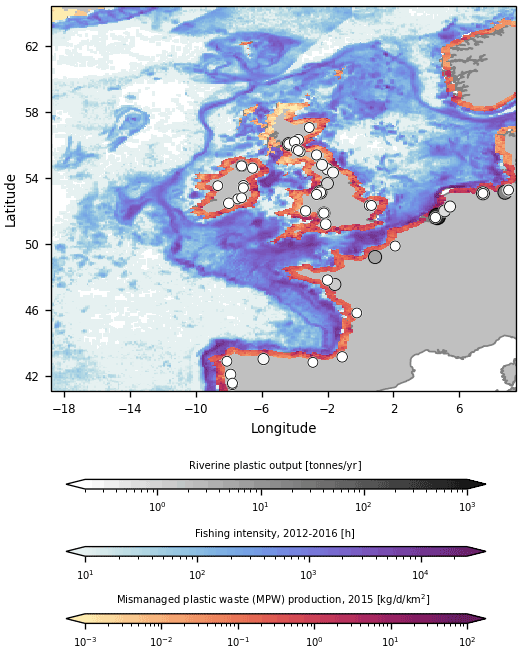
Figure 2Input scenarios used to seed virtual litter particles in the Lagrangian simulations. Riverine input is indicated by the green circles, the amount of fishing hours is shown in blue, and the coastal mismanaged plastic waste density is shown in red. Note the log scale used for all input scenarios. While all rivers from Lebreton et al. (2017) are included in our analysis, only rivers predicted to transport more than 0.2 t of plastic litter into the ocean are plotted here.
3.1.3 Coastal orientation and geometry
Coastal orientation, geometry, and substrate are likely to influence the amount of litter that actually beaches on coastlines (Brennan et al., 2018; Andrades et al., 2018; Hardesty et al., 2017). Although the substrate of beaches in the Netherlands is relatively similar (sandy), there are local variations in the coastline orientation with respect to the large-scale coastline. We take this into account by including information on how the hydrodynamic and wind data are oriented with respect to the local coastline.
The Natural Earth data set is used here at a 1:10 million resolution (Kelso and Patterson, 2010), which is fine enough to estimate the general orientation of the beaches on which the cleanup stages have taken place. Two locations are not present in the coastal geometry of this data set (two constructed beaches along dams: Brouwersdam and Neeltje Jans); the coastal orientations of these locations were determined manually.
Normal vectors to the coastline (denoted by n) are estimated by fitting a tangent plane through the points defining the coastline segments. Using a singular value decomposition we minimize the orthogonal distance between these points and the plane. All points within a box of 10×10 km centered around the stage midway point are selected (roughly the length scale of the beach cleanup tours). One example is plotted in Fig. 3a, where the dotted box is the selection around the stage midway point, and the coastline segments within this box are indicated in orange. The resulting normal vector to this coastline segment is plotted using the orange arrow.
Dot products are calculated for vector fields (e.g., current velocity) with respect to the coastline normal vectors to quantify how much a vector points onshore (positive dot product) or offshore (negative dot product). An example is presented in Fig. 3b. At a given stage midway point, the numerical data within a certain radius are selected. For each of the cells we can then calculate the dot product of the vector data with respect to the coastline normal vector. In the example of Fig. 3b, the normal vector points towards the northeast. Cells where the velocity vector points in roughly the same direction (onshore) are colored red, the opposite directions (offshore) are colored blue. In Fig. 3b the example is presented for only one time snapshot: the quantities can be calculated for various lead times. We then save derived quantities such as the mean, maximum, or minimum dot product over the lead time in a given radius, which will be further explained in Sect. 3.2.1.
The coastal normal vectors are also used to estimate the misalignment between the numerical model coastline and the high resolution coastline. In Fig. 3a, the numerical model grid cell centers at the coast are plotted using the brown dots. A singular value decomposition is used again to estimate the coastline normal vector of the numerical grid (ngrid, indicated by the brown arrow). At each stage midway point, the dot product is taken of ngrid with respect to the high-resolution coastline normal vector n to obtain a measure for the misalignment. In the example plotted in Fig. 3a there would be a large amount of misalignment between ngrid and n, resulting in a negative dot product between the two quantities.
Finally, the coastline length per grid cell is estimated. For each cell of the numerical model, we take the coastline segments within the given cell and calculate their total length. Since coastlines show fractal behavior (Kappraff, 1986) their Euclidian length is not well defined. This means that the lengths calculated here are estimates and that their value would increase when taking a higher model resolution.
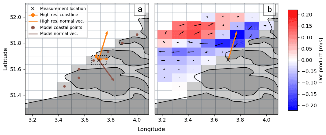
Figure 3Illustration of the methodology used to calculate the directional variables. Panel (a) shows the high-resolution coastline points and the derived normal vector (n), shown in orange, located around the stage midway point (the black cross). Also shown are the numerical model coastline points and the derived normal vector (ngrid) in brown. Panel (b) shows how the dot product variables are calculated. In a radius around the stage midway point, the dot product of the vector field is calculated with respect to the high-resolution coastline normal vector (n), where offshore components are indicated in blue and onshore components are shown in red.
3.1.4 Spatial variability
Information about spatial variability of beached litter can be useful for cleanup campaigns to target areas that are likely to be the most polluted. One might expect that cleanup locations close to each other show more similar litter concentrations compared to locations that are further apart. Furthermore, it is important for modeling studies to know the subgrid-scale variability that is not captured by the (discrete) numerical data (Kaandorp et al., 2020). Finally, observing how spatial variability changes for different length scales could give us clues which physical processes are important for the dispersion of litter.
We will quantify the spatial variability of litter found on the coast as a function of the separation distance between the different cleanup locations using an empirical variogram. To compute the empirical variogram, all pairs of measurements within a certain distance of each other are compared, defined by h±δ, where h is the separation distance and δ is half the bin width used to discretize the separation distance. The empirical variance of the measurements separated by h±δ is calculated using (Bachmaier and Backes, 2011)
where N(h±δ) denotes the number of samples in the given separation distance bin and z is the quantity of interest.
We calculate the empirical variogram on the log10 values of the measured plastic concentrations (in kg km−1). Confidence intervals of the calculated variogram are estimated using a jackknife parameter estimation (Shafer and Varljen, 1990).
Measured litter concentrations are subject to both spatial and temporal variability. To remove temporal variability as much as possible from the empirical variance estimates, we only use data pairs within a certain time separation. Decreasing the time separation window reduces the effect of the temporal variability but also reduces the number of available data pairs. We use a time separation of 3 d here, for which it was found that there are still enough available data pairs to compute the empirical variogram.
3.2 Model
3.2.1 Machine learning features
The variables described in Sect. 3.1.1–3.1.3 are used to create a set of explanatory variables, which are related to the observed beach litter quantities. It is, however, not obvious what kind of lead time should be considered for the variables and over which spatial scale the variables will have an influence on beach littering. We therefore calculate a large set of combinations for the explanatory variables by varying the radius of influence and/or the lead time. For the radii, we will consider the variable data closest to the stage midway point (which we will denote by a radius of 0 km) and variable data within radii of 50 and 100 km. For lead times, we will consider 1, 3, 9, and 30 d. As shown in Eriksson et al. (2013) and Ryan et al. (2014), the turnover of litter on beaches generally happens within timescales of days, meaning that with this range of lead times we should be able to capture most of the litter accumulation. Furthermore, a lead time of 30 d also captures all tidal variability up to and including the spring–neap cycle. The combinations of variables, lead times, and radii will be called features and are fed into the regression algorithm.
An overview of the features is given in Table 2. Three categories are defined: scalar features, directional features (which contain information on the direction of various vector fields with respect to the coastline), and features derived from the Lagrangian model simulations.
For the scalar features, we look at Hs and the magnitude of UStokes, Uwind, Ucurr., and Utides. We calculate the mean and the maximum of these quantities using all data points within the given radii and lead times.
We calculate a number of features derived from the tidal height htide. First of all, the maximum tidal height and the standard deviation of the tidal height over the given lead times are calculated, taking the closest data point from the stage midway point. Furthermore, a quantity is defined giving information in which period of the spring–neap tidal cycle the stage was monitored (htide,deriv.). The maximum tidal height at the stage day and the maximum tidal height at the given lead time are calculated. We calculate the temporal derivative by subtracting both values and dividing by the lead time. A positive value means we are approaching the spring tide, a negative value means we are approaching the neap tide. Since spring tides occur roughly every 2 weeks, only lead times of 1 and 3 d are used for this feature. Finally, the minimum and maximum tidal height encountered during each stage are calculated since these might contribute to how much beach was sampled during that day.
The total coastline length within a given radius is calculated (lcoast) using the Natural Earth data set, as explained in Sect. 3.1.3. To include possible local sources of litter, the population within a given radius (npop.) is included as a feature (SEDAC et al., 2005), as is the total fishing activity (Kroodsma et al., 2018) within a given radius (nfis.). Additionally, we want to include information about whether river mouths are present upstream of the cleanup stage. We use salinity (S) as a proxy for this, as low salinity indicates a nearby river mouth. The mean and minimum salinity are calculated over the various radii and lead times.
The number of participants for each stage is used as a feature (npart.) to assess whether a lower percentage of litter is captured at stages with less participants. These data are available for 2017–2019. For 2014–2016 only the total number of participants per year is available. To estimate the number of participants per stage for these years, we first calculate the participant fractions per location over 2017–2019. These fractions are then scaled with the total number of participants over 2014–2016.
For the directional features, we calculate the dot product of the Stokes drift, wind, ocean currents, and tides with respect to the coastline normal vector (n). The mean and maximum are again calculated (as is the minimum) since this gives us additional information as to whether there have been strong offshore components. These features are calculated for all radii and lead times. Furthermore, the misalignment of the numerical model coastline normal vector (ngrid) with respect to the coastline normal vector is specified as a feature.
Finally, the total fluxes of beached litter from the Lagrangian particle simulations are given as features from fisheries (Fbeach,fis.), riverine input (Fbeach,riv.), and mismanaged waste from the coastal population (Fbeach,pop.). These features are calculated for different beaching timescales τbeach, all radii, and all lead times. The features are divided by the appropriate lcoast corresponding to the radius to get the estimated beached litter fluxes per unit length of coast. One benefit of adding beached litter fluxes from the Lagrangian particle simulations is that potential sources of litter far away from the beaching location can be included. While the radius of influence for all features goes up to 100 km, the Lagrangian model features can still include information from further away, since the virtual particles are tracked indefinitely, as explained in Sect. 3.1.2.
Table 2An overview of the machine learning features used. For each set of variables in each column, derived quantities are calculated, e.g., the maximum, sum, or mean, over the given radius and lead time. Directional features are dot products of a given vector field with respect to the coastline normal vector n. For the last category (Lagrangian model features), the radius, lead time, and the beaching timescale (τbeach) are all varied.

*Further explanation is given in the main text for these parameters.
3.2.2 Regression model
The features and corresponding response (the measured amount of litter in kg km−1) are used to fit a random forest regression algorithm (Pedregosa et al., 2011). This model allows us to capture nonlinear relations between the features and response. It is a non-parametric model and does not require prior knowledge on the model structure. These are both important reasons to choose the specific algorithm: coastal processes affecting dispersion of marine litter are highly complex (van Sebille et al., 2020), and thus we do not know a priori how the different environmental variables might interact or how nonlinear these interactions might be. The random forest regression model can aid in scientific knowledge discovery (Bortnik and Camporeale, 2021) as it gives us Gini importance values for all features (Nembrini et al., 2018). This is another reason for choosing this specific algorithm, as it provides us information about which processes are important for predicting beached litter concentrations.
In total we have 342 features from all variable, radius, and lead time combinations. There are a total of 175 measured litter concentrations. The large number of features in comparison to the measurements makes it difficult to interpret the feature importance and could lead to overfitting. Therefore, k-fold cross-validation is used to validate and test the model on a reduced amount of features, which are selected from a set of clusters.
Some features correlate because they are derived from the same variable but for a different radius or lead time. However, we do not know a priori which of these radii and lead times are the most appropriate predictors for the beached litter quantities. For example, litter concentrations might be influenced by long-term processes, there may be a slow increase to the standing stock of litter on the beach, or the concentrations simply could be better predicted by conditions on the day leading up to the cleanup stage. Since we do not know whether these factors play a role, we let the algorithm select the most appropriate variables. Features that are highly correlated will be assigned to clusters. We use hierarchical Ward linkage clustering for this, based on Spearman rank–order correlations (McCann et al., 2019; Cope et al., 2017). As a result, the total set of features is reduced to 66 feature clusters. For further details and an interpretation of the clusters, see Appendix C.
Nested 5-fold cross-validation is used for optimal feature selection from the clusters and to assess the model performance on a test data set. In the outer loop, we use 80 % of the data to train the model and use the remaining 20 % to test the model performance. This is repeated for each fold, i.e., 5 times. In the inner loop, 80 % of the training data (i.e., 64 % of the total data) are used to train the model and 20 % (i.e., 16 % of the total data) are used to calculate the importance of the features; this process is also repeated 5 times. Since in the inner loop none of the test data are used to train the model, we do not overpredict the model performance (Hastie et al., 2008). As all features in our regression model are continuous (i.e., there is no bias from categorical features Nembrini et al., 2018) we use the random forest Gini importance. After the inner loop is complete, we then select the feature with the highest Gini importance from each cluster. The random forest is trained using the selected features, and its performance is evaluated using the test data. We keep track of which features from the clusters are estimated to be the most important. The entire process is repeated 10 times to obtain consistent feature importance estimates. A schematic of the model pipeline is presented in Appendix D.
4.1 Regression analysis
The regression model shows reasonable correspondence with the measured litter concentrations, where the Pearson correlation coefficient (R) based on the repeated cross-validation is 0.72±0.08. A scatterplot with the measured litter concentrations on the x axis and the predicted litter concentrations on the y axis is shown in Fig. 4. The points are colored according to their test folds. As the 5-fold cross-validation is repeated 10 times, only one realization is shown here, where every data point is plotted once.
In Fig. 4, the variability is shown that can be expected for length scales and timescales smaller than the numerical data resolution. Using the empirical variogram, we calculate that for lag distances of km. This lag distance is at the lower side of the grid resolution for the numerical data (approximately 7 km for the ocean current data), and thus the model is not able to capture variations below this length scale. Therefore, a 1:1 line is plotted for ±2 standard deviations based on this variance as an indication of the optimal performance that can be expected. In this case, 94 % of the predicted values lie inside the ±2σ interval, indicating that the model is close to the optimal performance that can be expected for the given spatial and temporal resolution. It can be seen that there are two kinds of outliers in Fig. 4: low observed litter concentrations not captured by the model (points in the upper left corner of the scatterplot) and high observed litter concentrations not captured by the model (points in the lower right corner of the scatterplot). This can be explained by the fact that the model is not able to capture all variability contained in the observations. As the hydrodynamic and wind data in the model have a limited resolution, subgrid-scale effects are missing (see Sect. 4.2). Furthermore, local point sources of litter (both spatially and temporally, e.g., shipping container accidents van der Molen et al., 2021) are not captured by the model.
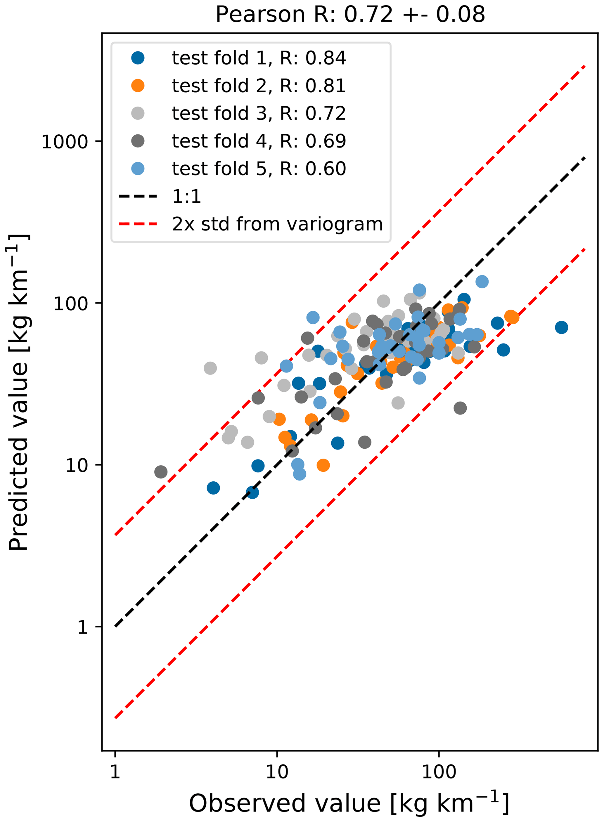
Figure 4Scatterplot of the observed log-transformed litter quantities (x axis) and the modeled log-transformed litter quantities (y axis). The points are colored according to the five test folds used in the analysis. The 1:1 line is plotted using the dashed black line, and the estimated uncertainty based on the small-scale variance (±2σ) is plotted using the dashed red lines.
In Fig. 5 we show box plots for the 10 most important features based on the Gini importance, which have been picked out of the total 66 feature clusters. Importance scores for all 66 feature clusters are plotted in Appendix B. The model indicates that tides play an important role for predicting the amount of beached litter. The most important feature is related to the long-term variability of the tidal height, with a lead time of 30 d. Short-term behavior is also seen as important, as the second most important feature is the maximum tidal height encountered within a lead time of 3 d. Furthermore, the maximum tidal height encountered during the tour is the sixth most important feature, and the dot product of the tidal currents with respect to the coastline is the eighth most important feature. In general, higher tidal maximum and variability lead to less litter measured on the coastline (see Appendix B5 for further details). A higher tide during or preceding the cleanup could resuspend some of the litter from the beach. Furthermore, a higher tide encountered during the cleanup stage reduces the beach width that can be sampled. Perhaps a stronger variability in the tidal height leads to less persistent high strandlines where the highest litter concentrations are normally found (Heo et al., 2013). It has been shown in numerical studies that residual tidal currents can lead to a net transport of both suspended and floating matter (Gräwe et al., 2014; Børve et al., 2021; Schulz and Umlauf, 2016). While the regression model indicates that tides play an important role, it is difficult to separate the causal relations between all these different effects and the litter quantities found on beaches. To quantify this in more detail, further experimental and numerical studies are required.
The coastline length in the neighborhood of the cleanup stage (lcoast) is ranked as the fourth most important feature. This feature can describe multiple effects on litter concentrations. More coastline per unit area means that litter concentrations are possibly spread out over longer stretches of beach, reducing the amount of litter per kilometer of beach. Furthermore, an increasing lcoast indicates an increasing irregularity of the nearby coastline shape. This is, for example, the case around the province of Zeeland in the southwest (<52∘ N in Fig. 1): in regions with irregular coastlines, more sheltered beaches can be found compared to regions with a long straight coastline, influencing the litter concentrations. Coastal orientation, ngrid⋅n, plays an important role given that it has the fifth-highest Gini importance. When the coastline section tends to be more directly located towards the open sea, the large-scale coastal geometry (ngrid) aligns with the small-scale coastal geometry (n) at the locations used here. In Haarr et al. (2019) and Hardesty et al. (2017), for example, it was reported that large-scale headlands tend to enhance catchment of litter compared to large-scale sheltered areas. This is in line with our findings, with an increasing ngrid⋅n leading to more predicted litter (see Appendix B5).
Results suggest that transport of marine litter is important to take into account, as the third and seventh most important features are beaching fluxes from the Lagrangian model simulations from fishing activity and coastal mismanaged waste, respectively. These features implicitly contain information about various hydrodynamic variables and sources of litter, explaining why these are ranked above most other scalar and directional features related to wind, currents, and waves. It is also interesting that they are all ranked above the nearby fishing activity (nfis.) and population density (npop.), which are the 10th and 14th most important features, respectively (see Fig. B1). This could indicate that transport of litter through the marine environment is important to take into account, as opposed to only considering local terrestrial sources. From the three possible sources of litter used in the model, transport from fisheries is the most important. This is consistent with the litter composition found on Dutch beaches, which consists in large part of fishing-related items (40 % van Duinen et al., 2021).
Finally, the dot product of Ucurr. with respect to the coastline is seen as important (ninth most important). This feature is related to small-scale and long-term behavior, which might give an indication as to whether there are currents present moving the litter onshore to the cleanup stage location.
Changes in predictive capability are relatively small when leaving out the Lagrangian model simulation features; see Fig. B2. The Pearson correlation coefficient R in this case is 0.72±0.10, which is not significantly lower than the full model. This suggests that information on transport of litter is to some extent also contained in other variables, such as the currents, waves, and wind magnitude and direction. Directional information seems to play an important role, as when leaving out the Lagrangian model simulation features, 4 out of the 10 most important features are related to the dot products of currents, tides, and Stokes drift with respect to the coastline (see Fig. B3).
It is estimated that the number of participants taking part in the tour does not have a large influence on the amount of litter that is found; see Appendix B for further details. This suggests that with an average of 77 participants per campaign, adding more participants would not necessarily lead to more litter being cleaned up. No clear patterns emerge regarding lead times and radii for the most important features. This could indicate that litter found on beaches is an ensemble of objects with different moments of beaching and residence times. Features regarding wind and significant wave height are seen as less important, being ranked 18th and lower; see Fig. B1. It is possible that this information is already contained in the Stokes drift or that they play a lesser role in the transport of litter. One explanation is that most of the litter found during the cleanup tour has a relatively low wind drag coefficient in the water, which was also observed in Lebreton et al. (2018) for litter in the Great Pacific Garbage Patch.
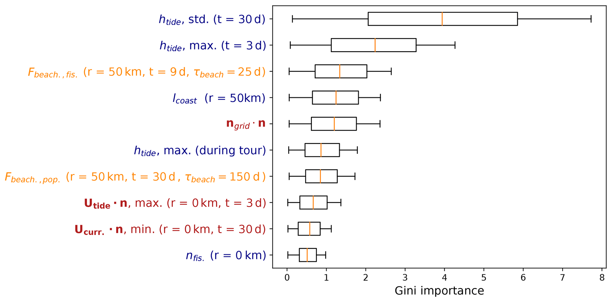
Figure 5Box plots for the feature Gini importance values from the random forest regression algorithm. Only the top 10 features are plotted here; an overview of all features can be found in Appendix B. The label colors correspond to the variable categories in Table 2, where scalar features are indicated in blue, directional features are shown in red, and Lagrangian model features are shown in orange. The radius and lead time are indicated in the brackets (when applicable).
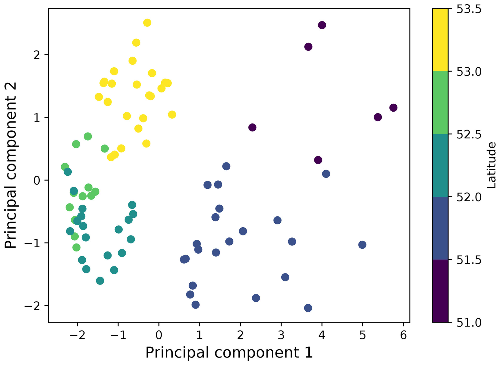
Having the full set of 66 feature clusters is not necessary for predictive capability. In Fig. B4 we show that the model performs well when only picking the top eight features (Pearson correlation coefficient R: 0.79±0.04). Increasing the amount of features does not increase the model performance. For an operational model it would therefore be recommended to stick to a lower amount of features, as this keeps the model simple and easier to interpret. We investigate if the most important variables are related to certain locations by performing a principal component analysis, taking these eight most important features in the full model (Fig. 5). A scatterplot of the first two principal components is presented in Fig. 6, where the dots are colored according to their latitude. The two principal components explain 50 % and 17 % of the total variance, respectively. What can be seen is that the points separate into roughly three different regions: measurements taken at lower latitudes around the province of Zeeland (51–52∘ N), measurements taken between 52 and 53∘ N, and measurements obtained near the Wadden Islands (53–53.5∘ N). The first principal component shows the highest absolute correlation (Pearson R: 0.45) with long-term tidal variability (with a lead time of 30 d). The second principal component shows the highest absolute correlation (Pearson R: −0.58) with the nearby coastal length (within a radius of 50 km). As the measurements taken between 52–53∘ N are clustered quite closely together, this indicates that conditions regarding tides and coastline geometry are relatively similar for these locations. Variations in the tidal height are relatively large between 51–52∘ N. The coastal geometry is also more irregular here compared to the rest of the Netherlands. These factors combined likely lead to less litter on beaches here: calculated over 2014–2019 for <52∘ N we find on average 52 kg km−1, and for >52∘ N we find on average 73 kg km−1 for the same period.
4.2 Spatial variability
To assess which length scales are important for the spatial variability of beached litter, we calculate the empirical variogram for different lag distances. Spatial variability remains relatively constant for lag distances up to about 100 km, with a mean of ; see Fig. 7. For the smallest lag distance ( km), we find . This variance estimate was also used to create the error bars in Fig. 4. Around h=125 km there seems to be an increase in the variance to about –0.3. However, at this lag distance there is also a large uncertainty in the estimates and fewer unique data pairs to calculate the empirical variance.
Interestingly, some periodic behavior seems to be present with a length scale of about 25 km. One possible explanation could be the typical spacing of the Dutch islands and peninsulas. As shown in the previous section, coastline orientation likely plays an important role in the amount of observed litter. This effect can also present itself in the variogram with, for example, measurements in sheltered areas (e.g., coves) being more correlated with each other compared to nearby exposed locations (e.g., headlands).
The grid sizes used for our numerical data range from about 7 km (the surface current data) to about 20 km (the wind data). This means that the variance at and below these length scales is not captured by the numerical data. The variance calculated for lag distances up to 20 km is quite substantial (–0.12). As can be seen in Fig. 4 the values corresponding to the lower and upper 95 % confidence interval vary by about an order of magnitude. This is essential to consider when using observational data to inform numerical models: due to the amount of variability at the subgrid-scale level, relatively large sets of observational data are required to extract information. A large number of physical processes could induce variability below length scales of 20 km, such as Langmuir circulations or processes in the coastal zone such as wave breaking, rip currents, and alongshore currents (van Sebille et al., 2020). Finally, it is important to consider that spatial variability is inherent to data obtained from cleanup campaigns such as those analyzed here, due to, e.g., different participants having slightly different strategies for finding litter on beaches.
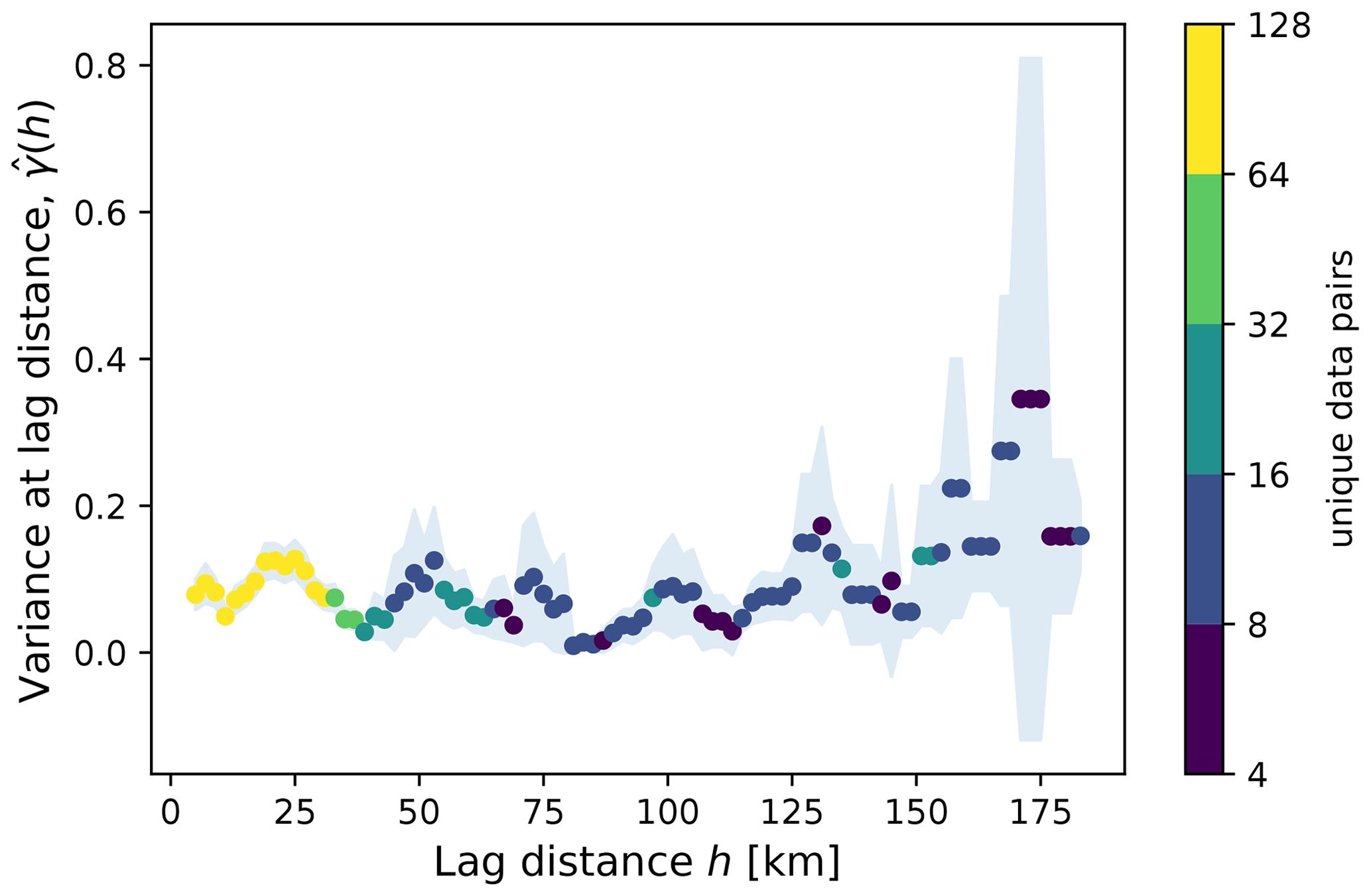
Figure 7Variogram calculated for the log10 of the measured litter quantities (in kg km−1), with the lag distance h on the x axis and the empirical variance on the y axis. Only data pairs with a maximum of 3 d temporal separation are taken into account. For the separation distance half bin width δ=5 km is used. The points are colored by the number of unique data pairs used to calculate the variance, and the jackknife uncertainty estimate (±σ) is shaded in blue.
4.3 Extrapolating litter quantities to the entire coastline
The random forest regression model can be used to extrapolate how much litter is likely to be beached along the entire Dutch coastline. First, a regression model is trained using the top eight features listed in Fig. 5. We then divide the Dutch North Sea coastline into sections (roughly 7 km by 7 km). For each of the sections the top eight features are computed, as well as the total coastline length contained in each section. In total we have 65 separate sections and a total coastline length of 365 km, which matches the total length of the Dutch North Sea coastline from the literature (Roomen et al., 2008). We choose to use a model trained using the top eight features for the extrapolations, as increasing the amount of features does not increase the predictive performance (see Fig. B4). Furthermore, reducing the amount of features simplifies the computations, as we do not need to compute all 391 variables again for all coastline sections.
For each section, the litter concentrations (in kg km−1) are predicted per day over the month of August in the years 2014–2019. Predictions are only made for August since all cleanup campaigns were organized during this period, and thus making predictions for other months might induce seasonal biases. The mean concentrations per coastline section are plotted in Fig. 8. For each day, the total litter quantities are computed by multiplying the litter concentrations by the coastline length per section. Monte Carlo estimates of the confidence bounds are calculated by randomly adding noise proportional to the estimated variance (), which is repeated 1000 times per day per section.
We find a total of 16 500–31 200 kg litter along the Dutch North Sea coastline based on the 95 % confidence interval. It must be noted that this only accounts for the visible litter on the beach surface. The cleanup efforts are likely to miss a substantial amount of beached litter that is buried in beach sediment or located at the back of the beach (e.g., in vegetation). This was also noted, for example, in Lavers and Bond (2017) for a remote island in the South Pacific, where in terms of mass about 68 % of the litter was located on the beach surface, 27 % was found at the back of the beach in and around vegetation, and 5 % was buried in beach sediment. Further research is necessary to quantify how these numbers translate to Dutch beaches.
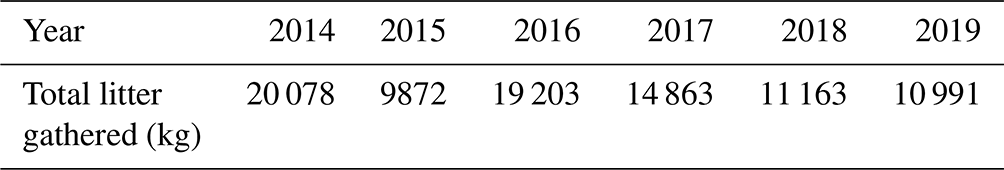
The total amount of litter gathered during the cleanup campaigns and the total amount of kilometers sampled per year is presented in Table A1. The total amount of litter gathered varies from 9872 to 20 078 kg. This is in line with the expected total amount of litter predicted by the model, since the majority of the coastline (222–262 km out of 365 km) was covered during the cleanup campaigns.
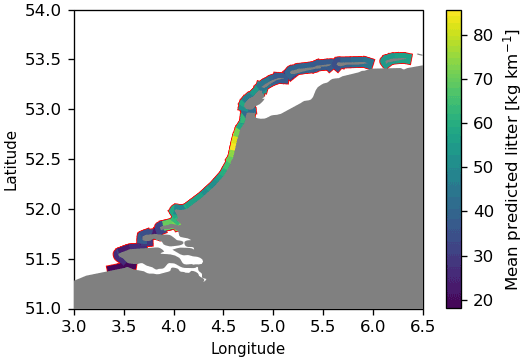
Figure 8Mean litter concentrations over the month of August in the years 2014–2019 extrapolated to the entire Dutch coastline.
Using data from beach cleanup efforts in the Netherlands for the years 2014–2019, we analyzed which variables are important for predicting litter on beaches and what spatial variability this litter has. In order to do this, we fitted a regression model to the observed litter quantities as a function of variables related to wind, waves, currents, tides, coastal geometry, and simulated oceanic transport. We find that tides play an important role, where increasing tidal variability and increasing tidal maximum lead to less observed litter on beaches. Other important variables are whether the local orientation of a beach corresponds to the large-scale coastline orientation and the total nearby coastal length, which can both be seen as measures of how exposed a beach is. These factors are likely explanations for why the observed litter quantities are relatively low in the southwestern part of the Netherlands compared to the other parts. Additionally, transport of litter through the marine environment is seen as important to take into account by the regression model. Rivers, fishing activity, and mismanaged plastic waste along coastlines were taken into account as possible sources of litter in the transport model, where the regression analysis attributed relatively high importance to litter originating from fishing activity. This is in line with findings in van Duinen et al. (2021), as approximately 40 % of the litter found on the Dutch North Sea coastline is estimated to originate from the fishing industry.
We compute that spatial variability of the observed litter concentrations is substantial on length scales less than 10 km, causing model ±2σ confidence bounds to vary by about an order of magnitude. Due to this significant variability, large observational data sets are necessary if they are to be used to inform numerical models. Finally, based on extrapolation of the regression model, we estimate that the Dutch North Sea coastlines contain a total of 16 500–31 200 kg (95 % confidence interval) of litter on the beach surface.
Estimating the spatial variability of beached litter can give us information for efficient monitoring of pollution. It can be used to constrain estimates of litter concentrations based on observations elsewhere. We found that the variance for lag distances smaller than 125 km is relatively constant around . As an example, if one measures a relatively high amount of 200 kg km−1 at the northern tip of the mainland near Den Helder (≈53∘ N in Fig. 1), one can expect at least 54 kg km−1 of litter elsewhere in the northern part of the Netherlands, taking the 95 % confidence interval. After 125 km, the estimated variance seems to increase, meaning that this observation becomes less informative for locations further away.
For future studies on quantifying beach litter variability, it would be interesting to segment the beach cleanup tours into smaller stretches. One idea would be to organize some stages where the litter quantities are weighed per 1 km, 100 m, or even shorter stretches. This way it would be possible to estimate the variance on sub-kilometer scale. Ryan et al. (2020) reported significant correlations between measurements taken roughly 50 m apart (Spearman rank correlation of about 0.9). It would be interesting to see how this changes up to the kilometer scale. This can give us valuable insights into which processes might be causing the high amount of variability between litter observations and what length scales should be taken into account to capture this variability with models. We see relatively few data points in Fig. 7 for larger lag distances. Performing the cleanup stages in a randomized order would provide a more even coverage of data points over the given lag distances.
Future studies could further investigate the causal relations between the variables seen as important predictors by the regression model and the litter concentrations found on beaches. This is especially the case for tides, which constitute the two most important features in the regression model (see Fig. 5). Experimental studies could further determine whether lower litter concentrations at locations with higher tidal variability are mainly caused by litter re-suspending back into the sea or (for example) due to the fact that less area of the beach is sampled during high tide. It should additionally be investigated how these effects compare to the role of (residual) tidal currents, as it has been shown that this can play an important role in transporting suspended matter towards the shore (Schulz and Umlauf, 2016). Experimental investigations can be done in combination with numerical studies of the nearshore marine environment to capture the interactions between processes such as tides, waves, and particle sizes (Alsina et al., 2020).
It should be investigated how the results found here generalize to other geographic regions, and how the importance of explanatory variables vary globally. The model itself cannot be directly used for other geographic regions since the features used to train the algorithm are specific to the region of interest. The model is likely to perform poorly when making extrapolations for conditions not present in the training data. As an example, the substrate of beaches is likely to have a large impact on litter concentrations (Hardesty et al., 2017), which are relatively uniform in this analysis (all sandy beaches). According to our regression model, wind is not a very important variable to take into account. Perhaps some of the high-windage litter has been beached before reaching the Dutch waters. It should be noted, however, that wind indirectly affects other variables such as the ocean currents, and it therefore also affects the Lagrangian particle simulations. It would be interesting to redo this analysis with data obtained in the nearby English channel and check if wind plays a more important role there, as in the Lagrangian model simulations many virtual particles pass through this region.
It is necessary to further investigate the effect of regular cleaning of beaches by municipalities and other volunteer groups or individuals. This effect was left out in this analysis due to unavailability of these data. It is likely that it is mainly the beaches near densely populated areas that are regularly cleaned. Since data on population density has been included in the features, it is possible that this effect is taken into account by the regression model, but further analysis is necessary. Furthermore, effects of tourism can be taken into account in the future when these data are available, as this affects the local population density seasonally.
Regarding effective cleanup of beaches, it is recommended to perform beach cleanups during low tide, preferably in a week around the neap tide, when the tidal variability is lower. If limited resources are available, one can focus on exposed shorelines, which generally accumulate more litter. Additionally, more litter can be expected on relatively straight shorelines compared to more irregular geometries where litter is distributed over longer stretches of beach. We saw no effect from the number of participants per beach cleanup tour on the amount of gathered litter, with an average of 77 participants per tour. One possible improvement to clean up more litter could therefore be to spread out participants over different stages, avoiding parts of the beach being inspected multiple times.
Figures A1 and A2 present the modeled litter quantities (left column) and the raw observational data (right column) per year per cleanup stage. The litter concentrations are plotted using circles, where the color and size correspond to the litter quantities (note the logarithmic scale here). Table A1 presents the total gathered litter per year.
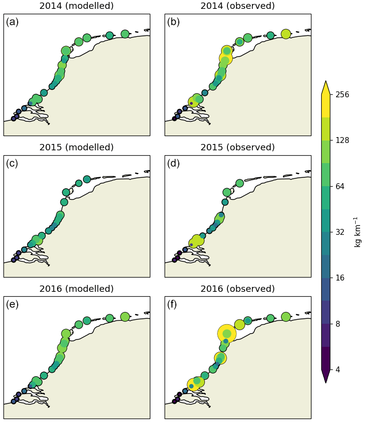
Figure A1Modeled (a) and observed (b) litter concentrations (in kg km−1) per individual location and year (2014–2016). Circles are scaled and colored according to the litter concentrations.
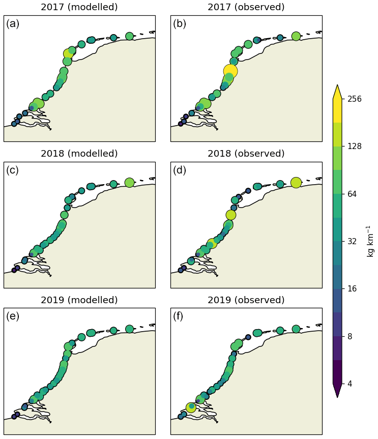
Figure A2Modeled (a) and observed (b) litter concentrations (in kg km−1) per individual location and year (2017–2019). Circles are scaled and colored according to the litter concentrations.
Table A1Overview of the total amount of litter gathered per year during the beach cleanup tours.
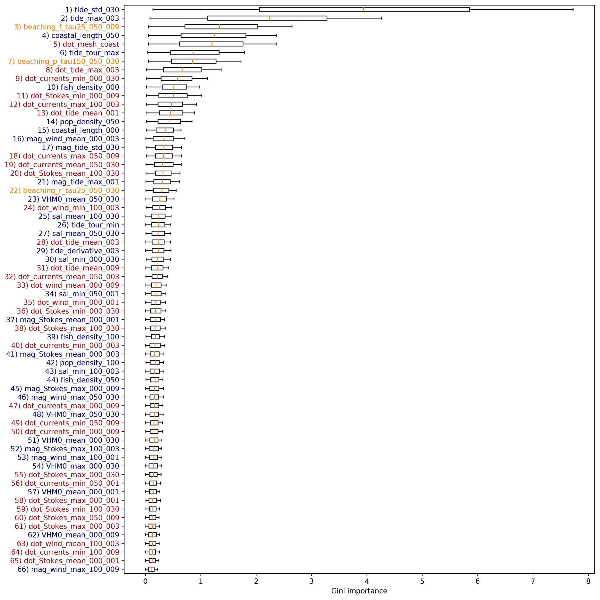
B1 Gini importance overview
A complete overview of the Gini importance for all features is presented in Fig. B1. The numbers in the feature labels give information about the radius (in kilometers) and lead time (in days) if applicable. See Table 2 for the radius and lead time combinations used for the variables. The Lagrangian model features (orange labels) are indicated by “beaching_p”, “beaching_r”, and “beaching_f”, for litter sources originating from mismanaged coastal plastic waste (p), rivers (r), and fishing activity (f), respectively.
B2 Excluding Lagrangian model features
A scatterplot of the measured litter concentrations versus the predicted values is presented in Fig. B2, where Lagrangian model features have been excluded from the feature set. As described in the main text, no significant decrease in the correlation is observed compared to the case where Lagrangian model features have been included (0.70±0.10 versus 0.71±0.11).

Figure B2Scatterplot of the observed litter quantities (x axis), and the modeled litter quantities (y axis), when not taking Lagrangian model features into account. Litter quantities are log-transformed, and points are colored according to the five test folds used in the analysis.
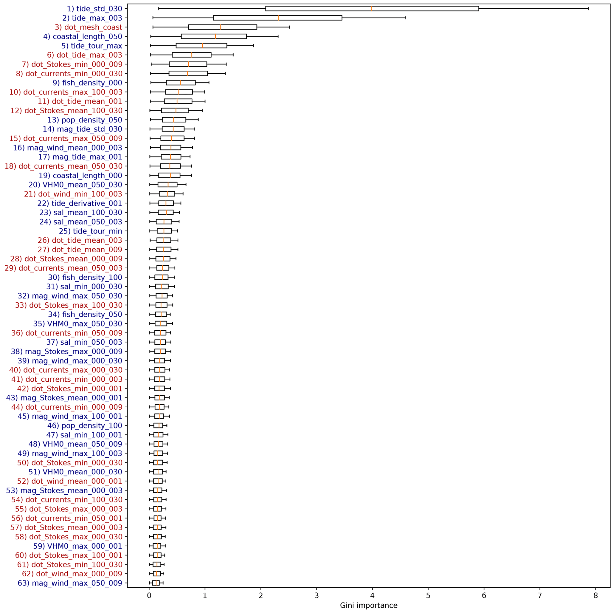
A complete overview of the featured Gini importance values corresponding to the cases without Lagrangian model features is presented in Fig. B3. As mentioned in the main text, more features related to the currents and Stokes drift orientation with respect to the coastline are seen as important here when compared to Fig. B1. This could be explained due to these features taking over the role of the Lagrangian model features in capturing the effect of marine litter transport.
B3 Effect of using only the top N features
It is not necessary to include all 66 feature clusters for predictive capability of the model. In Fig. B4 we present the Pearson correlation coefficient R as a function of the number of features included in the random forest algorithm both with and without using the Lagrangian model features. Each time only the top features (corresponding to Figs. B1 and B3) are used to train and test the model, using 5-fold cross-validation repeated 10 times. Generally the model performs well when about 7–8 features used. Performance is quite stable in cases where Lagrangian model features are used; some outliers with lower Pearson correlation coefficients can be observed when not taking into account these features. The Pearson correlation coefficient when using all 66 features, corresponding to Fig. 4, is shown using the red error bar. In this case the Pearson correlation coefficient is slightly smaller than when using, for example, the top eight features, which could indicate a small amount of overfitting, although this difference is not significant.
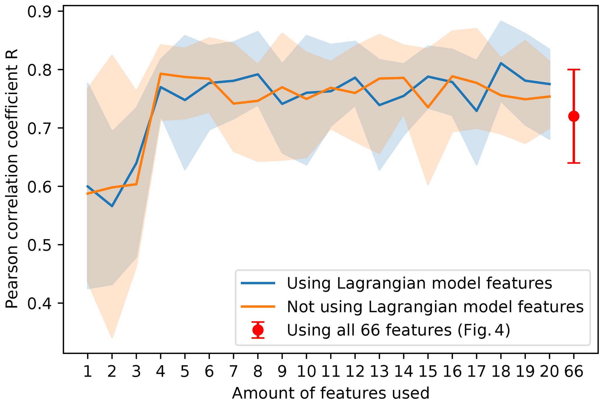
Figure B4The effect of the number of included features on the Pearson correlation coefficient R, where the mean is plotted using the solid line, and the filled area represents the 10 % to 90 % quantile. Cases both with and without using Lagrangian model features are presented (blue and orange lines, respectively). The case using all 66 features (corresponding to Fig. 4) is shown using the red error bar.
In Fig. B5, we analyze the effect of leaving out certain feature categories on the model performance. The random forest can create a highly nonlinear map between the features and corresponding response. It is therefore possible that when using a large set of features and leaving out one important explanatory variable, it will use a combination of the remaining features to still obtain a good fit. We therefore only use the top 10 features in this analysis and exclude the Lagrangian model variables, as these implicitly contain information on the other features. As can be seen, leaving out a certain category of features reduces the model performance. This can especially be observed when leaving out all features regarding tides and the two features regarding coastal properties (lcoast and ngrid⋅n). The mean Pearson correlation coefficient decreases, and the variance of the model performance increases.
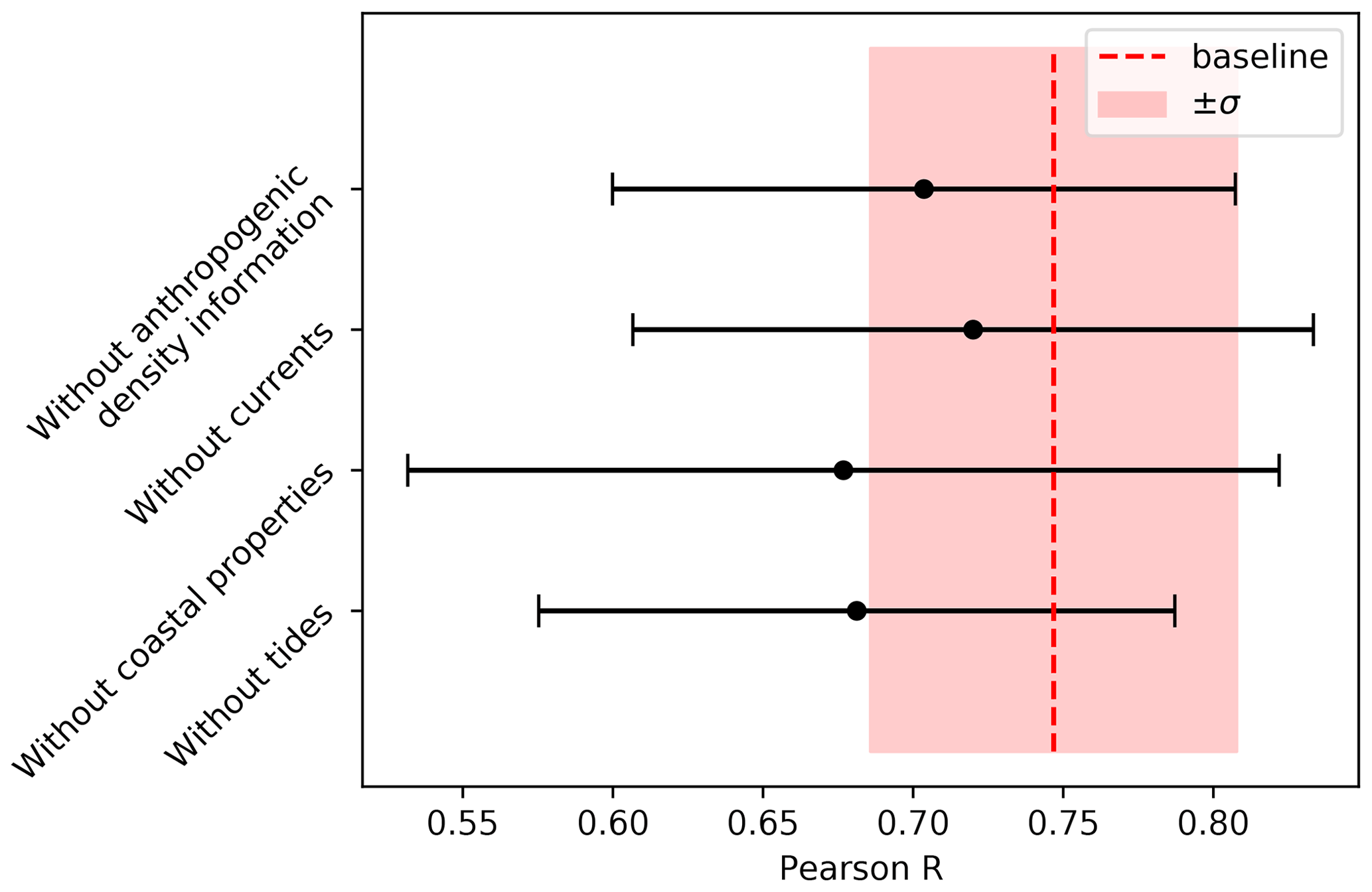
Figure B5Analysis where some of the feature categories have been left out. The top 10 features have been used without the Lagrangian model features (see Fig. B3) as these implicitly contain information on all feature categories. As can be observed, leaving out a set of features generally decreases the predictive performance of the model and increases the variability of the prediction quality.
B4 Number of participants
As mentioned in the main text, the number of participants is not seen as important in terms of the Gini importance. The number of participants is correlated with the population density in the neighborhood of the stage and is therefore assigned to the same feature cluster as the population density; for more details see Appendix C. The number of participants was not picked out of this cluster as one of the most important features during the k-fold cross-validation. In order to separate the effect of the number of participants per cleanup stage, a model run was done without the nearby population densities being used as features. A summary of the resulting Gini importance values is shown in Fig. B6, where only the top 10 features and the number of participants are plotted.
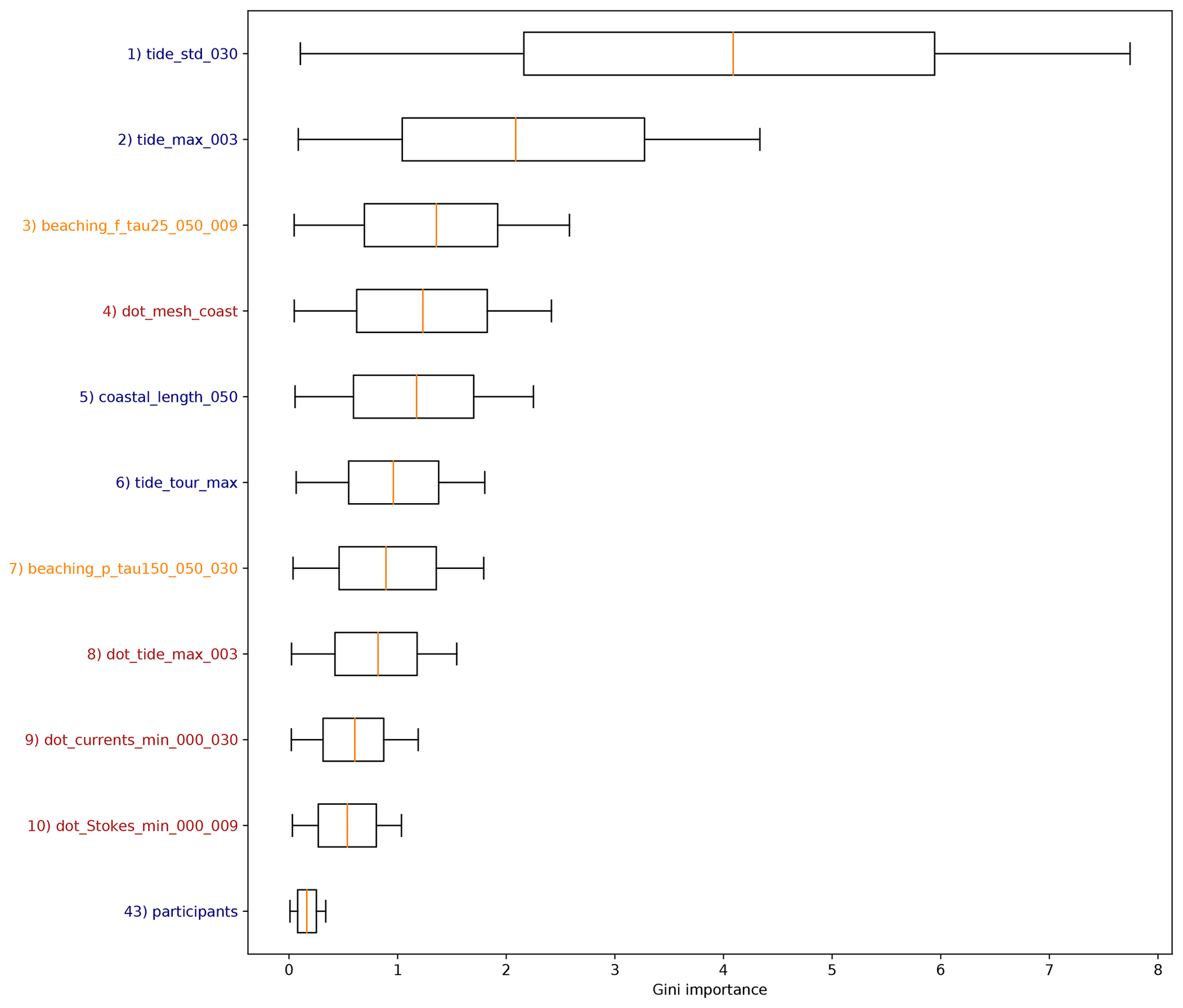
Figure B6Gini importance overview when not using nearby population densities as features, which separates the effect of the number of participants per cleanup stage. In this case, it is the 28th most important feature.
B5 Feature effect
The general effect of some features was described in the main text, such as the fact that an increasing tidal variability, and misalignment of the high resolution coastline with respect to the numerical model coastline (ngrid⋅n) lead to less observed litter. Figure B7 illustrates this by varying one feature on the x axis and plotting the resulting predictions on the y axis. In the decision trees of the random forest, decision boundaries are made at optimal splitting locations, making the resulting model highly nonlinear. This makes it difficult to interpret the regression model. In Fig. B7, we “fix” all features except the one listed on the x axis. This feature is then varied from its minimum until its maximum encountered value. Since the random forest result can depend highly on the exact value of the other features, noise is introduced. Each other feature is varied uniformly between its 0.4–0.6 quantile to illustrate whether the found relation for the given feature on the x axis is robust.
Features which show relatively robust relations are related to tidal height, where an increasing variability and a higher maximum decrease the predicted litter concentrations. The effect for ngrid⋅n also seems to be robust, with increasing values leading to more predicted litter. For the coastal length in the neighborhood (lcoast) an increasing value seems to lead to less litter, although there is a sudden drop observed here. This might be caused by the fact that there are relatively few data points available where this feature has a high value (most of the stages were conducted on relatively straight coastline sections), and thus the model has trouble learning a relation here. For the Lagrangian model features, increasing values lead to more predicted litter, as expected. For the mismanaged coastal plastic waste (indicated by “beaching_p_tau25_050_009”), the results are quite dependent on the values of other features, as a lot of noise can be seen here. Generally, the model indicates there are increasing litter concentrations for increasing currents and onshore Stokes drift.
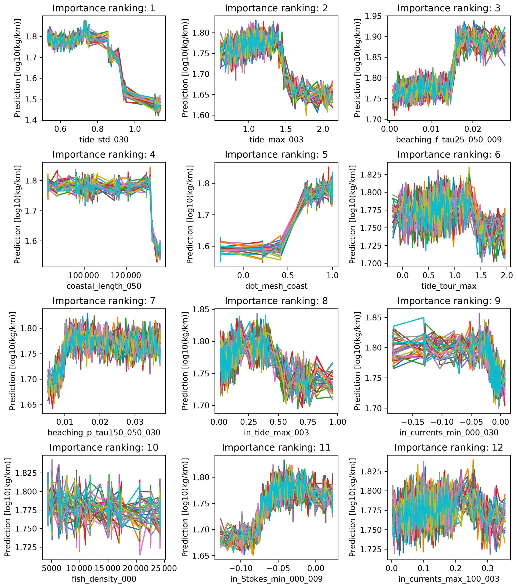
Figure B7Illustrated effect of the 12 most important features (x axes) on the litter concentrations (y axes) according to the random forest regression model. For the 12 most important features, we vary their value from the minimum to maximum encountered value. All other features are fixed, and some noise is added to illustrate robustness of the relations.
Correlated features are put into clusters using hierarchical Ward linkage clustering (McCann et al., 2019; Cope et al., 2017). An overview of the resulting dendrogram is shown in Fig. C1. A threshold is chosen to make a cut in the dendrogram. This was selected by hand to be a value of 2.3, at which the clusters remain relatively interpretable (e.g., separate clusters for coastal properties and tidal properties). The cut is shown in the figure by the dashed red line. Some general patterns regarding the clusters are indicated in the dendrogram.
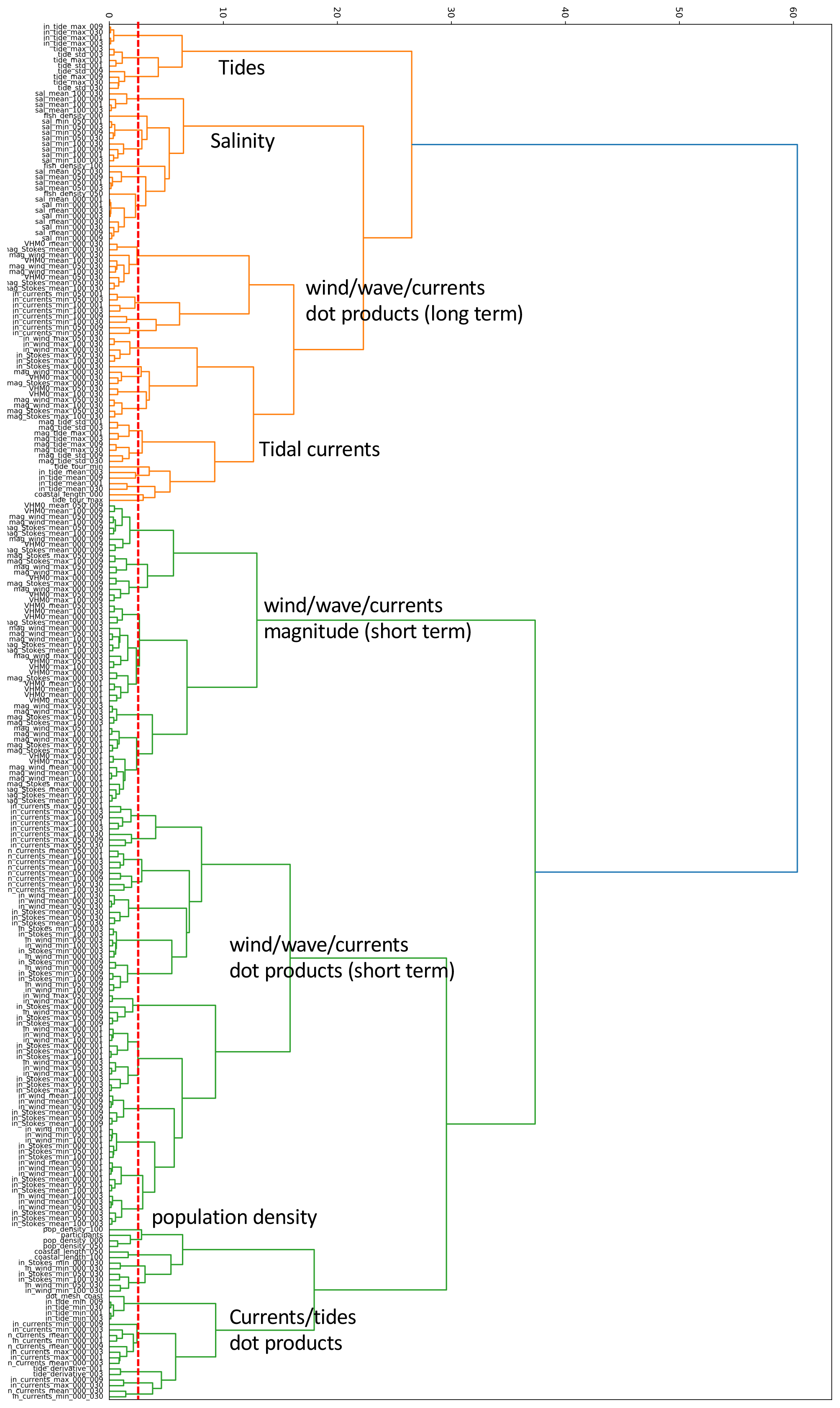
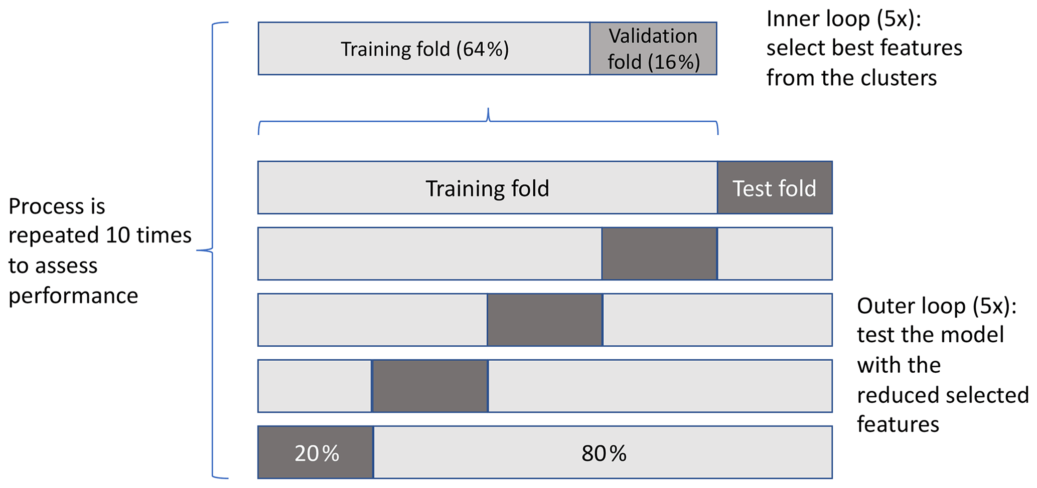
Figure D1Pipeline to train and test the random forest regression model. Nested k-fold cross-validation is used to select the best feature from each cluster (inner loop) and to evaluate the model trained with the best features of the test data set (outer loop). The process is repeated to assess the average performance.
Code used to conduct the experiment and to create all of the figures and the beach cleanup data from Stichting De Noordzee are available at https://doi.org/10.24416/UU01-NVGL3G (Kaandorp et al., 2021b).
MLAK designed and conducted the study, with initial data analysis from EvS and steering and discussion from EvS, SLY, MB, and HAD. Curation of the beach cleanup tour data was done by MB. All authors contributed to the manuscript.
Marijke Boonstra is employed by the North Sea Foundation. All other authors declare no competing interests.
Publisher's note: Copernicus Publications remains neutral with regard to jurisdictional claims in published maps and institutional affiliations.
The North Sea Foundation thanks all volunteers that participated in the Beach Cleanup Tour. We also like to thank all sponsors and partners that make the Beach Cleanup Tour possible.
This work was supported through funding from the European Research Council (ERC) under the European Union Horizon 2020 research and innovation programme (grant agreement no. 715386). Funding was provided to Stefanie L. Ypma by the Galapagos Conservation Trust and the Evolution Education Trust, Pathways to Sustainability, and the K.F. Hein Fonds.
This paper was edited by Oliver Zielinski and reviewed by three anonymous referees.
Alsina, J. M., Jongedijk, C. E., and van Sebille, E.: Laboratory Measurements of the Wave-Induced Motion of Plastic Particles: Influence of Wave Period, Plastic Size and Plastic Density, J. Geophys. Res.-Oceans, 125, e2020JC016294, https://doi.org/10.1029/2020JC016294, 2020. a
Andrades, R., Santos, R. G., Joyeux, J. C., Chelazzi, D., Cincinelli, A., and Giarrizzo, T.: Marine debris in Trindade Island, a remote island of the South Atlantic, Mar. Pollut. Bull., 137, 180–184, https://doi.org/10.1016/j.marpolbul.2018.10.003, 2018. a
Andrady, A. L.: Microplastics in the marine environment, Mar. Pollut. Bull., 62, 1596–1605, https://doi.org/10.1016/j.marpolbul.2011.05.030, 2011. a
Bachmaier, M. and Backes, M.: Variogram or Semivariogram? Variance or Semivariance? Allan Variance or Introducing a New Term?, Math. Geosci., 43, 735–740, https://doi.org/10.1007/s11004-011-9348-3, 2011. a
Balas, C. E., Ergin, A., Williams, A. T., and Koc, L.: Marine litter prediction by artificial intelligence, Mar. Pollut. Bull., 48, 449–457, https://doi.org/10.1016/j.marpolbul.2003.08.020, 2004. a
Bortnik, J. and Camporeale, E.: Ten Ways to Apply Machine Learning in Earth and Space Sciences, Eos, 102, https://doi.org/10.1029/2021EO160257, 2021. a
Børve, E., Isachsen, P. E., and Nøst, O. A.: Rectified tidal transport in Lofoten–Vesterålen, northern Norway, Ocean Sci., 17, 1753–1773, https://doi.org/10.5194/os-17-1753-2021, 2021. a
Brennan, E., Wilcox, C., and Denise, B.: Science of the Total Environment Connecting flux , deposition and resuspension in coastal debris surveys, Sci. Total Environ., 644, 1019–1026, https://doi.org/10.1016/j.scitotenv.2018.06.352, 2018. a, b
Cope, T. E., Wilson, B., Robson, H., Drinkall, R., Dean, L., Grube, M., Jones, P. S., Patterson, K., Griffiths, T. D., Rowe, J. B., and Petkov, C. I.: Artificial grammar learning in vascular and progressive non-fluent aphasias, Neuropsychol., 104, 201–213, https://doi.org/10.1016/j.neuropsychologia.2017.08.022, 2017. a, b
Critchell, K. and Lambrechts, J.: Modelling accumulation of marine plastics in the coastal zone; what are the dominant physical processes?, Eastuar. Coast. Shelf S., 171, 111–122, https://doi.org/10.1016/j.ecss.2016.01.036, 2016. a
Critchell, K., Grech, A., Schlaefer, J., Andutta, F., Lambrechts, J., Wolanski, E., and Hamann, M.: Modelling the fate of marine debris along a complex shoreline: Lessons from the Great Barrier Reef, Eastuar. Coast. Shelf S., 167, 414–426, https://doi.org/10.1016/j.ecss.2015.10.018, 2015. a
De Ruijter, W. P., Visser, A. W., and Bos, W. G.: The Rhine outflow: A prototypical pulsed discharge plume in a high energy shallow sea, J. Mar. Syst., 12, 263–276, https://doi.org/10.1016/S0924-7963(96)00102-9, 1997. a
Delandmeter, P. and van Sebille, E.: The Parcels v2.0 Lagrangian framework: new field interpolation schemes, Geosci. Model Dev., 12, 3571–3584, https://doi.org/10.5194/gmd-12-3571-2019, 2019. a
Eriksson, C., Burton, H., Fitch, S., Schulz, M., and van den Hoff, J.: Daily accumulation rates of marine debris on sub-Antarctic island beaches, Mar. Pollut. Bull., 66, 199–208, https://doi.org/10.1016/j.marpolbul.2012.08.026, 2013. a, b, c, d
Global Monitoring and Forecasting Center: Global Ocean Waves Reanalysis WAVERYS product, E.U. Copernicus Marine Service Information [data set], https://resources.marine.copernicus.eu/?option=com_csw&view=details&product_id=GLOBAL_REANALYSIS_WAV_001_032 (last access: 10 February 2021), 2020. a
Global Monitoring and Forecasting Center: Atlantic-European North West Shelf Ocean Physics Reanalysis product, E.U. Copernicus Marine Service Information [data set], https://resources.marine.copernicus.eu/?option=com_csw&view=details&product_id=NWSHELF_MULTIYEAR_PHY_004_009 (last access: 8 March 2021), 2021. a, b, c, d
Granado, I., Basurko, O. C., Rubio, A., Ferrer, L., Hernández-González, J., Epelde, I., and Fernandes, J. A.: Beach litter forecasting on the south-eastern coast of the Bay of Biscay: A bayesian networks approach, Cont. Shelf Res., 180, 14–23, https://doi.org/10.1016/j.csr.2019.04.016, 2019. a
Gräwe, U., Burchard, H., Müller, M., and Schuttelaars, H. M.: Seasonal variability in M2 and M4 tidal constituents and its implications for the coastal residual sediment transport, Geophys. Res. Lett., 41, 5563–5570, https://doi.org/10.1002/2014GL060517, 2014. a, b
Haarr, M. L., Westerveld, L., Fabres, J., Iversen, K. R., and Busch, K. E. T.: A novel GIS-based tool for predicting coastal litter accumulation and optimising coastal cleanup actions, Mar. Pollut. Bull., 139, 117–126, https://doi.org/10.1016/j.marpolbul.2018.12.025, 2019. a, b, c, d
Haarr, M. L., Pantalos, M., Hartviksen, M. K., and Gressetvold, M.: Citizen science data indicate a reduction in beach litter in the Lofoten archipelago in the Norwegian Sea, Mar. Pollut. Bull., 153, 111000, https://doi.org/10.1016/j.marpolbul.2020.111000, 2020. a
Hardesty, B. D., Lawson, T. J., van der Velde, T., Lansdell, M., and Wilcox, C.: Estimating quantities and sources of marine debris at a continental scale, Front. Ecol. Environ., 15, 18–25, https://doi.org/10.1002/fee.1447, 2017. a, b, c, d
Hastie, T., Tibshirani, R., and Friedman, J.: The Elements of Statistical Learning, Springer, 2 Edn., ISBN 978-0-387-84857-0, 2008. a
Hengstmann, E., Gräwe, D., Tamminga, M., and Fischer, E. K.: Marine litter abundance and distribution on beaches on the Isle of Rügen considering the influence of exposition, morphology and recreational activities, Mar. Pollut. Bull., 115, 297–306, https://doi.org/10.1016/j.marpolbul.2016.12.026, 2017. a
Heo, N. W., Hong, S. H., Han, G. M., Hong, S., Lee, J., Song, Y. K., Jang, M., and Shim, W. J.: Distribution of small plastic debris in cross-section and high strandline on Heungnam beach, South Korea, Ocean Sci. J., 48, 225–233, https://doi.org/10.1007/s12601-013-0019-9, 2013. a
Hersbach, H., Bell, B., Berrisford, P., Hirahara, S., Horányi, A., Muñoz‐Sabater, J., Nicolas, J., Peubey, C., Radu, R., Schepers, D., Simmons, A., Soci, C., Abdalla, S., Abellan, X., Balsamo, G., Bechtold, P., Biavati, G., Bidlot, J., Bonavita, M., Chiara, G., Dahlgren, P., Dee, D., Diamantakis, M., Dragani, R., Flemming, J., Forbes, R., Fuentes, M., Geer, A., Haimberger, L., Healy, S., Hogan, R. J., Hólm, E., Janisková, M., Keeley, S., Laloyaux, P., Lopez, P., Lupu, C., Radnoti, G., Rosnay, P., Rozum, I., Vamborg, F., Villaume, S., and Thépaut, J.: The ERA5 global reanalysis, Q. J. Roy. Meteor. Soc., 146, 1999–2049, https://doi.org/10.1002/qj.3803, 2020. a, b, c
Hidalgo-Ruz, V. and Thiel, M.: Distribution and abundance of small plastic debris on beaches in the SE Pacific (Chile): A study supported by a citizen science project, Mar. Environ. Res., 87, 12–18, https://doi.org/10.1016/j.marenvres.2013.02.015, 2013. a
Jambeck, J. R., Geyer, R., Wilcox, C., Siegler, T. R., Perryman, M., Andrady, A., Narayan, R., and Law, K. L.: Plastic waste inputs from land into the ocean, Science, 347, 768–771, https://doi.org/10.1126/science.1260352, 2015. a
Kaandorp, M. L. A., Dijkstra, H. A., and van Sebille, E.: Closing the Mediterranean Marine Floating Plastic Mass Budget: Inverse Modeling of Sources and Sinks, Environ. Sci. Tech., 54, 11980–11989, https://doi.org/10.1021/acs.est.0c01984, 2020. a, b, c, d, e
Kaandorp, M. L. A., Dijkstra, H. A., and van Sebille, E.: Modelling size distributions of marine plastics under the influence of continuous cascading fragmentation, Environ. Res. Lett., 16, 54075, https://doi.org/10.1088/1748-9326/abe9ea, 2021a. a
Kaandorp, M. L. A., Ypma, S., Boonstra, M., Dijkstra, H. A., and van Sebille, E.: Code and data for the Dutch North Sea beached litter analysis, [code, data], https://doi.org/10.24416/UU01-NVGL3G, 2021b. a
Kappraff, J.: The Fractal Geometry of coastlines: a study in fractals, Comp. Maths. Appls., 12, 655–671, 1986. a
Kelso, N. V. and Patterson, T.: Introducing Natural Earth Data – Naturalearthdata.com, Geogr. Tech., 82–89, 2010. a
Koelmans, A. A., Kooi, M., Law, K. L., and van Sebille, E.: All is not lost: Deriving a top-down mass budget of plastic at sea, Environ. Res. Lett., 12, 114028, https://doi.org/10.1088/1748-9326/aa9500, 2017. a
Kordella, S., Geraga, M., Papatheodorou, G., Fakiris, E., and Mitropoulou, I. M.: Litter composition and source contribution for 80 beaches in Greece, Eastern Mediterranean: A nationwide voluntary clean-up campaign, Aquat. Ecosyst. Health Manage., 16, 111–118, https://doi.org/10.1080/14634988.2012.759503, 2013. a
Kroodsma, D. A., Mayorga, J., Hochberg, T., Miller, N. A., Boerder, K., Ferretti, F., Wilson, A., Bergman, B., White, T. D., Block, B. A., Woods, P., Sullivan, B., Costello, C., and Worm, B.: Tracking the global footprint of fisheries, Science, 359, 904–908, https://doi.org/10.1126/science.aao5646, 2018. a, b
Lavers, J. L. and Bond, A. L.: Exceptional and rapid accumulation of anthropogenic debris on one of the world's most remote and pristine islands, P. Natl. Acad. Sci. USA, 114, 6052–6055, https://doi.org/10.1073/pnas.1619818114, 2017. a
Lebreton, L., Slat, B., Ferrari, F., Sainte-Rose, B., Aitken, J., Marthouse, R., Hajbane, S., Cunsolo, S., Schwarz, A., Levivier, A., Noble, K., Debeljak, P., Maral, H., Schoeneich-Argent, R., Brambini, R., and Reisser, J.: Evidence that the Great Pacific Garbage Patch is rapidly accumulating plastic, Sci. Rep., 8, 1–15, https://doi.org/10.1038/s41598-018-22939-w, 2018. a, b
Lebreton, L., Egger, M., and Slat, B.: A global mass budget for positively buoyant macroplastic debris in the ocean, Sci. Rep., 9, 12922, https://doi.org/10.1038/s41598-019-49413-5, 2019. a, b
Lebreton, L. C., Van Der Zwet, J., Damsteeg, J. W., Slat, B., Andrady, A., and Reisser, J.: River plastic emissions to the world's oceans, Nat. Commun., 8, 1–10, https://doi.org/10.1038/ncomms15611, 2017. a, b
Lyard, F. H., Allain, D. J., Cancet, M., Carrère, L., and Picot, N.: FES2014 global ocean tide atlas: design and performance, Ocean Sci., 17, 615–649, https://doi.org/10.5194/os-17-615-2021, 2021. a
Macias, D., Cózar, A., Garcia-gorriz, E., González-fernández, D., and Stips, A.: Surface water circulation develops seasonally changing patterns of fl oating litter accumulation in the Mediterranean Sea . A modelling approach, Mar. Pollut. Bull., 149, 110619, https://doi.org/10.1016/j.marpolbul.2019.110619, 2019. a
McCann, A., Jeffery, I. B., Ouliass, B., Ferland, G., Fu, X., Booth, S. L., Tran, T. T., O'Toole, P. W., and O'Connor, E. M.: Exploratory analysis of covariation of microbiota-derived Vitamin K and cognition in older adults, Am. J. Clin. Nutr., 110, 1404–1415, https://doi.org/10.1093/ajcn/nqz220, 2019. a, b
Morales-Caselles, C., Viejo, J., Martí, E., González-Fernández, D., Pragnell-Raasch, H., González-Gordillo, J. I., Montero, E., Arroyo, G. M., Hanke, G., Salvo, V. S., Basurko, O. C., Mallos, N., Lebreton, L., Echevarría, F., van Emmerik, T., Duarte, C. M., Gálvez, J. A., van Sebille, E., Galgani, F., García, C. M., Ross, P. S., Bartual, A., Ioakeimidis, C., Markalain, G., Isobe, A., and Cózar, A.: An inshore–offshore sorting system revealed from global classification of ocean litter, Nat. Sustain., 4, 484–493, https://doi.org/10.1038/s41893-021-00720-8, 2021. a, b
Moy, K., Neilson, B., Chung, A., Meadows, A., Castrence, M., Ambagis, S., and Davidson, K.: Mapping coastal marine debris using aerial imagery and spatial analysis, Mar. Pollut. Bull., 132, 52–59, https://doi.org/10.1016/j.marpolbul.2017.11.045, 2018. a
Nembrini, S., König, I. R., and Wright, M. N.: The revival of the Gini importance?, Bioinformatics, 34, 3711–3718, https://doi.org/10.1093/bioinformatics/bty373, 2018. a, b
Neumann, D., Callies, U., and Matthies, M.: Marine litter ensemble transport simulations in the southern North Sea, Mar. Pollut. Bull., 86, 219–228, https://doi.org/10.1016/j.marpolbul.2014.07.016, 2014. a
Newman, S., Watkins, E., Farmer, A., Brink, P. T., and Schweitzer, J.-P.: The Economics of Marine Litter, in: Marine Anthropogenic Litter, edited by: Bergmann, M., Gutow, L., and Klages, M., Springer International Publishing, Cham, 367–394, https://doi.org/10.1007/978-3-319-16510-3{_}14, 2015. a
Ogunola, O. S., Onada, O. A., and Falaye, A. E.: Mitigation measures to avert the impacts of plastics and microplastics in the marine environment (a review), Environ. Sci. Pollut. Res., 25, 9293–9310, https://doi.org/10.1007/s11356-018-1499-z, 2018. a
Onink, V., Jongedijk, C. E., Hoffman, M. J., van Sebille, E., and Laufkötter, C.: Global simulations of marine plastic transport show plastic trapping in coastal zones, Environ. Res. Lett., 16, 064053, https://doi.org/10.1088/1748-9326/abecbd, 2021. a, b, c
Pawlowicz, R.: The Grounding of Floating Objects in a Marginal Sea, J. Phys. Oceanogr., 51, 537–551, https://doi.org/10.1175/jpo-d-20-0183.1, 2020. a, b
Pedregosa, F., Varoquaux, G., Gramfort, A., Michel, V., Thirion, B., Grisel, O., Blondel, M., Prettenhofer, P., Weiss, R., Dubourg, V., Vanderplas, J., Passos, A., Cournapeau, D., Brucher, M., Perrot, M., and Duchesnay, E.: Scikit-learn: Machine Learning in Python, J. Mach. Learn. Res., 12, 2825–2830, https://doi.org/10.5555/1953048.2078195, 2011. a
Rech, S., Macaya-Caquilpán, V., Pantoja, J., Rivadeneira, M., Jofre Madariaga, D., and Thiel, M.: Rivers as a source of marine litter – A study from the SE Pacific, Mar. Pollut. Bull., 82, 66–75, https://doi.org/10.1016/j.marpolbul.2014.03.019, 2014. a
Ribic, C. A., Sheavly, S. B., Rugg, D. J., and Erdmann, E. S.: Trends and drivers of marine debris on the Atlantic coast of the United States 1997-2007, Mar. Pollut. Bull., 60, 1231–1242, https://doi.org/10.1016/j.marpolbul.2010.03.021, 2010. a
Ribic, C. A., Sheavly, S. B., Rugg, D. J., and Erdmann, E. S.: Trends in marine debris along the U.S. Pacific Coast and Hawai'i 1998-2007, Mar. Pollut. Bull., 64, 994–1004, https://doi.org/10.1016/j.marpolbul.2012.02.008, 2012. a
Ricker, M. and Stanev, E. V.: Circulation of the European northwest shelf: a Lagrangian perspective, Ocean Sci., 16, 637–655, https://doi.org/10.5194/os-16-637-2020, 2020. a
Rijnsburger, S., Flores, R. P., Pietrzak, J. D., Horner‐Devine, A. R., Souza, A. J., and Zijl, F.: The Evolution of Plume Fronts in the Rhine Region of Freshwater Influence, J. Geophys. Res.-Oceans, 126, 1–28, https://doi.org/10.1029/2019jc015927, 2021. a
Roomen, M. V., Keijl, G., Koks, B., and Mostert, K.: Numbers of wintering waders on the North Sea coast of the Netherlands in January 1998, in: International Wader Studies, International Wader Study Group, Thetford, UK, 18, 55–58, 2008. a
Ryan, P. G., Lamprecht, A., Swanepoel, D., and Moloney, C. L.: The effect of fine-scale sampling frequency on estimates of beach litter accumulation, Mar. Pollut. Bull., 88, 249–254, https://doi.org/10.1016/j.marpolbul.2014.08.036, 2014. a
Ryan, P. G., Weideman, E. A., Perold, V., and Moloney, C. L.: Toward Balancing the Budget: Surface Macro-Plastics Dominate the Mass of Particulate Pollution Stranded on Beaches, Front. Mar. Sci., 7, 575395, https://doi.org/10.3389/fmars.2020.575395, 2020. a
Schulz, K. and Umlauf, L.: Residual transport of suspended material by tidal straining near sloping topography, J. Phys. Oceanogr., 46, 2083–2102, https://doi.org/10.1175/JPO-D-15-0218.1, 2016. a, b
Schulz, M. and Matthies, M.: Artificial neural networks for modeling time series of beach litter in the southern north sea, Mar. Environ. Res., 98, 14–20, https://doi.org/10.1016/j.marenvres.2014.03.014, 2014. a
SEDAC, CIESIN – Center for International Earth Science Information Network – Columbia University, FAO – United Nations Food and Agriculture Programme, and CIAT – Centro Internacional de Agricultura Tropical: Gridded Population of the World, Version 3 (GPWv3): Population Count Grid [data set], https://doi.org/10.7927/H4639MPP, 2005. a, b
Shafer, J. M. and Varljen, M. D.: Approximation of confidence limits on sample semivariograms from single realizations of spatially correlated random fields, Water Resour. Res., 26, 1787–1802, https://doi.org/10.1029/WR026i008p01787, 1990. a
Song, K., Jung, J. Y., Lee, S. H., and Park, S.: A comparative study of deep learning-based network model and conventional method to assess beach debris standing-stock, Mar. Pollut. Bull., 168, 112466, https://doi.org/10.1016/j.marpolbul.2021.112466, 2021. a
Sterl, M. F., Delandmeter, P., and Sebille, E.: Influence of Barotropic Tidal Currents on Transport and Accumulation of Floating Microplastics in the Global Open Ocean, J. Geophys. Res.-Oceans, 125, e2019JC015583, https://doi.org/10.1029/2019JC015583, 2020. a, b
Thepwilai, S., Wangritthikraikul, K., Chawchai, S., and Bissen, R.: Testing the factors controlling the numbers of microplastics on beaches along the western Gulf of Thailand, Mar. Pollut. Bull., 168, 112467, https://doi.org/10.1016/j.marpolbul.2021.112467, 2021. a, b
van der Molen, J., van Leeuwen, S. M., Govers, L. L., van der Heide, T., and Olff, H.: Potential Micro-Plastics Dispersal and Accumulation in the North Sea, With Application to the MSC Zoe Incident, Front. Mar. Sci., 8, 607203, https://doi.org/10.3389/fmars.2021.607203, 2021. a
van Duinen, B., Kaandorp, M. L. A., and van Sebille, E.: Identifying Marine Sources of Beached Plastics Through a Bayesian Framework: Application to Southwest Netherlands, Geophys. Res. Lett., 49, e2021GL097214, https://doi.org/10.1029/2021GL097214, 2021. a, b
van Sebille, E., Griffies, S. M., Abernathey, R., Adams, T. P., Berloff, P., Biastoch, A., Blanke, B., Chassignet, E. P., Cheng, Y., Cotter, C. J., Deleersnijder, E., Döös, K., Drake, H. F., Drijfhout, S., Gary, S. F., Heemink, A. W., Kjellsson, J., Koszalka, I. M., Lange, M., Lique, C., MacGilchrist, G. A., Marsh, R., Mayorga Adame, C. G., McAdam, R., Nencioli, F., Paris, C. B., Piggott, M. D., Polton, J. A., Rühs, S., Shah, S. H., Thomas, M. D., Wang, J., Wolfram, P. J., Zanna, L., and Zika, J. D.: Lagrangian ocean analysis: Fundamentals and practices, Ocean Model., 121, 49–75, https://doi.org/10.1016/j.ocemod.2017.11.008, 2018. a
van Sebille, E., Aliani, S., Law, K. L., Maximenko, N., Alsina, J. M., Bagaev, A., Bergmann, M., Chapron, B., Chubarenko, I., Cózar, A., Delandmeter, P., Egger, M., Fox-Kemper, B., Garaba, S. P., Goddijn-Murphy, L., Hardesty, B. D., Hoffman, M. J., Isobe, A., Jongedijk, C. E., Kaandorp, M. L. A., Khatmullina, L., Koelmans, A. A., Kukulka, T., Laufkötter, C., Lebreton, L., Lobelle, D., Maes, C., Martinez-Vicente, V., Morales Maqueda, M. A., Poulain-Zarcos, M., Rodríguez, E., Ryan, P. G., Shanks, A. L., Shim, W. J., Suaria, G., Thiel, M., van den Bremer, T. S., and Wichmann, D.: The physical oceanography of the transport of floating marine debris, Environ. Res. Lett., 15, 023003, https://doi.org/10.1088/1748-9326/ab6d7d, 2020. a, b, c
Williams, A. T. and Tudor, D. T.: Litter burial and exhumation: Spatial and temporal distribution on a cobble pocket beach, Mar. Pollut. Bull., 42, 1031–1039, https://doi.org/10.1016/S0025-326X(01)00058-3, 2001. a, b
Zettler, E. R., Takada, H., Monteleone, B., Mallos, N., Eriksen, M., and Amaral-Zettler, L. A.: Incorporating citizen science to study plastics in the environment, Anal. Meth., 9, 1392–1403, https://doi.org/10.1039/c6ay02716d, 2017. a
- Abstract
- Introduction
- Data description and region of interest
- Methodology
- Results and discussion
- Conclusions and recommendations
- Appendix A: Observational and modeled data per year
- Appendix B: Extended results
- Appendix C: Clustering dendrogram
- Appendix D: Model pipeline
- Code and data availability
- Author contributions
- Competing interests
- Disclaimer
- Acknowledgements
- Financial support
- Review statement
- References