the Creative Commons Attribution 4.0 License.
the Creative Commons Attribution 4.0 License.
 | 06 Oct 2021
Atmospherically forced sea-level variability in western Hudson Bay, Canada
Igor A. Dmitrenko
Denis L. Volkov
Tricia A. Stadnyk
Andrew Tefs
David G. Babb
Sergey A. Kirillov
Alex Crawford
Kevin Sydor
David G. Barber
In recent years, significant trends toward earlier breakup and later freeze-up of sea ice in Hudson Bay have led to a considerable increase in shipping activity through the Port of Churchill, which is located in western Hudson Bay and is the only deep-water ocean port in the province of Manitoba. Therefore, understanding sea-level variability at the port is an urgent issue crucial for safe navigation and coastal infrastructure. Using tidal gauge data from the port along with an atmospheric reanalysis and Churchill River discharge, we assess environmental factors impacting synoptic to seasonal variability of sea level at Churchill. An atmospheric vorticity index used to describe the wind forcing was found to correlate with sea level at Churchill. Statistical analyses show that, in contrast to earlier studies, local discharge from the Churchill River can only explain up to 5 % of the sea-level variability. The cyclonic wind forcing contributes from 22 % during the ice-covered winter–spring season to 30 % during the ice-free summer–fall season due to cyclone-induced storm surges generated along the coast. Multiple regression analysis revealed that wind forcing and local river discharge combined can explain up to 32 % of the sea-level variability at Churchill. Our analysis further revealed that the seasonal cycle of sea level at Churchill appears to be impacted by the seasonal cycle in atmospheric circulation rather than by the seasonal cycle in local discharge from the Churchill River, particularly post-construction of the Churchill River diversion in 1977. Sea level at Churchill shows positive anomalies for September–November compared to June–August. This seasonal difference was also revealed for the entire Hudson Bay coast using satellite-derived sea-level altimetry. This anomaly was associated with enhanced cyclonic atmospheric circulation during fall, reaching a maximum in November, which forced storm surges along the coast. Complete sea-ice cover during winter impedes momentum transfer from wind stress to the water column, reducing the impact of wind forcing on sea-level variability. Expanding our observations to the bay-wide scale, we confirmed the process of wind-driven sea-level variability with (i) tidal-gauge data from eastern Hudson Bay and (ii) satellite altimetry measurements. Ultimately, we find that cyclonic winds generate sea-level rise along the western and eastern coasts of Hudson Bay at the synoptic and seasonal timescales, suggesting an amplification of the bay-wide cyclonic geostrophic circulation in fall (October–November), when cyclonic vorticity is enhanced, and Hudson Bay is ice-free.
- Article
(12238 KB) - Full-text XML
-
Supplement
(1373 KB) - BibTeX
- EndNote


Hudson Bay in northeast Canada is a shallow (mean depth ∼150 m), semi-enclosed, sub-arctic inland sea that is connected to the Labrador Sea through Hudson Strait (Fig. 1). The bay occupies approximately 831 000 km2, making it the world's largest inland sea, and is characterized by a high annual volume of river discharge (712 km3; Déry et al., 2005, 2011) and a dynamic seasonal ice cover that exists from November–December to June–July (Hochheim and Barber, 2010, 2014). The mean circulation in Hudson Bay is comprised of the wind-driven and estuarine components, where the estuarine portion is driven by the riverine water input (Prinsenberg, 1986a), and the wind-driven portion is attributed to prevailing along-shore winds (e.g., Ingram and Prinsenberg, 1998; Saucier et al., 2004; St-Laurent et al., 2011; Ridenour et al., 2019a; Dmitrenko et al., 2020). Model simulations by Saucier et al. (2004) show that the cyclonic circulation is stronger during fall, reaching a maximum in November when the winds are strongest, and weakest in spring when Hudson Bay has a complete sea-ice cover. Dmitrenko et al. (2020), however, found that even during the ice-covered season strong cyclones can amplify water circulation in the bay. This is consistent with conclusions by St-Laurent et al. (2011), who noted that momentum is transmitted through the mobile ice pack to the water column. The efficiency of momentum transmission through the mobile ice strongly depends on sea-ice roughness, which is impacted by ice concentration and characteristic length scales of roughness elements including pressure ridges, melt ponds etc. (e.g., Lüpkes et al., 2012; Tsamados et al., 2014; Joyce et al., 2019). In particular, ice floes in a state of free drift within a partial or weak ice cover, typical of the polynya area in western Hudson Bay, increase the transfer of wind stress into the water column (Schulze and Pickart, 2012). Both velocity measurements (Prinsenberg, 1986b; Ingram and Prinsenberg, 1998; Dmitrenko et al., 2020) and model simulations (Wang et al., 1994; Saucier et al., 2004; St-Laurent et al., 2011; Ridenour et al., 2019b) show that during summer, cyclonic water circulation produces a coastal transport corridor that advects riverine water along the coast toward Hudson Strait and into the Labrador Sea.

Figure 1Map of Hudson Bay. Red dots depict the permanent tide gauge in Churchill and temporary tide gauges in Inukjuak, Cape Jones Island and North Kopak Island. Blue arrows highlight Churchill, Nelson, and Innuksuak river mouths. Blue crosses depict the five-point stencil used for computing atmospheric vorticity approximated as Laplacian from sea-level atmospheric pressure. The numbered black lines depict depth contours of 50, 100, 150, and 200 m. (a) Inset shows the Hudson Bay location within North America. The map of Hudson Bay was compiled based on the General Bathymetric Chart of the Oceans (GEBCO, https://www.gebco.net/, last access: 30 September 2021).
The local water mass of Hudson Bay is dominated by freshwater input comprised of river runoff from the largest watershed in Canada and sea-ice meltwater (e.g., Prinsenberg, 1984, 1988, 1991; Saucier and Dionne, 1998; Granskog et al., 2009; Eastwood et al., 2020). The annual mean discharge rate of 22.6×10³ m3 s−1 corresponds to a net discharge of 712 km3 of freshwater per year (Déry et al., 2005, 2011). A similar volume of 742±10 km3 of freshwater is contained within the ice pack by April (Landy et al., 2017). Freshwater transport in Hudson Bay exhibits a strong seasonal cycle influenced by the timing of river discharge (e.g., Déry et al., 2005), the annual melt–freeze cycle of sea ice (Ingram and Prinsenberg, 1998; Saucier et al., 2004; Straneo and Saucier, 2008; Granskog et al., 2011), and seasonality of wind forcing (Saucier et al., 2004; St-Laurent et al., 2011).
During the last decade, significant progress has been achieved in understanding the Hudson Bay environmental system (e.g., Granskog et al., 2009; Kuzyk et al., 2011; St-Laurent et al., 2011; Piecuch and Ponte, 2015; Landy et al., 2017; Kuzyk and Candlish, 2019; Eastwood et al., 2020; Dmitrenko et al., 2020, 2021). However, the synoptic, seasonal, and interannual variability of sea level in Hudson Bay still remains insufficiently studied due to a scarcity of sea-level observations at permanent tidal gauges. Note that the tidal gauge in Churchill (Fig. 1) is the only continuously operating tide gauge in Hudson Bay and the central Canadian Arctic. Historically, the focus of sea-level studies in Hudson Bay was motivated by this area's post-glacial isostatic rebound (e.g., Gutenberg, 1941; Tushingham, 1992); for a detailed review of these earlier studies see Wolf et al. (2006). The advent of space geodesy, in particular GPS, absolute gravimetry, and satellite altimetry measurements (e.g., Larson and van Dam, 2000; Wolf et al., 2006; Sella et al., 2007), afforded a shift in focus for Hudson Bay sea-level research to environmental aspects related to global warming and hydroelectric regulation (Gough, 1998, 2000), and those associated with increasing the shipping traffic from the Port of Churchill through Hudson Bay to Hudson Strait, which may soon become a federally designated transportation corridor (e.g., Andrews et al., 2017; Pew Charitable Trusts, 2016).
In 2016, the University of Manitoba and Manitoba Hydro launched a project on “Variability and change of freshwater-marine coupling in the Hudson Bay System”, named BaySys, which aimed to assess the relative contributions of climate change and river regulation to the Hudson Bay system. Here, we are specifically focused on the impact of the Churchill River diversion on variability of sea level at the Port of Churchill. Additionally, we put our findings in the context of wind forcing over the entire Hudson Bay, elaborating on the suggestion by Dmitrenko et al. (2020) that cyclonic wind forcing generates onshore Ekman transport and storm surges along the coast.
We also revisit earlier results by Gough and Robinson (2000) and Gough et al. (2005). Using tidal gauge and river discharge data from 1974 to 1994, Gough and Robinson (2000) suggested that the Churchill River discharge dominates sea-level variability at Churchill. They explained the seasonal elevation of sea level during late fall by a recirculating mechanism that links the spring pulse of river discharge in the downstream James Bay (Fig. 1) to sea level at Churchill (Gough and Robinson, 2000; Gough et al., 2005). In this paper, we present an alternative mechanism and show that (i) the Churchill River discharge plays a secondary role for generating sea-level anomalies (SLAs) at Churchill, and (ii) the synoptic and seasonal variability of sea level at Churchill and over the entire Hudson Bay is impacted by the wind forcing described with an atmospheric vorticity index (Fig. 2).

Figure 2(a) Time series of the monthly mean atmospheric vorticity index (s−1) over Hudson Bay, derived from NCEP (red) and ERA5 (blue). (b) Scatter plot of the monthly mean meridional wind seaward of Churchill in western Hudson Bay (m s−1) versus the monthly mean atmospheric vorticity index. Thick black line depicts linear regression. Numbers at the bottom show correlation R between (a) the monthly mean vorticity derived from NCEP (1949–2000) and ERA5 (1979–2000) and (b) the monthly mean NCEP vorticity versus meridional wind (1949–2020).
2.1 Sea level
The daily mean sea-level data used in this study were retrieved from the Canadian Tides and Water Levels Data Archive of the Fisheries and Oceans Canada through http://www.isdm-gdsi.gc.ca/isdm-gdsi/twl-mne/index-eng.htm#s5 (last access: 26 August 2021). Sea-level data were de-tided using an algorithm by Foreman (1977). Measurements of sea level at Churchill were obtained from the permanent tidal gauge that is installed at the port of Churchill (station no. 5010) near the mouth of the Churchill River (Fig. 1). While measurements of sea level at Churchill date back to the 1930s (Gutenberg, 1941), we only used data from 1950 to the present (Fig. 3a), which is coincident with atmospheric reanalysis data from the National Centers for Environmental Prediction (NCEP; Kalnay et al., 1996). In addition, we used sea-level data from the temporary tidal gauge in Inukjuak (station no. 4575), Cape Jones Island (station no. 4656), and North Kopak Island (station no. 4548) (Fig. 1). Among these three locations, only data at Inukjuak are fully representative for our analysis because they span a sufficiently long period from October 1969 to October 1980; however, only the portion of this time series from September 1973 to December 1975 is continuous. Sea-level records at Cape Jones Island and North Kopak Island are from August–October 1973 and 1975, respectively, and were selected among other temporary stations in Hudson Bay to overlap with sea-level time series at Inukjuak.
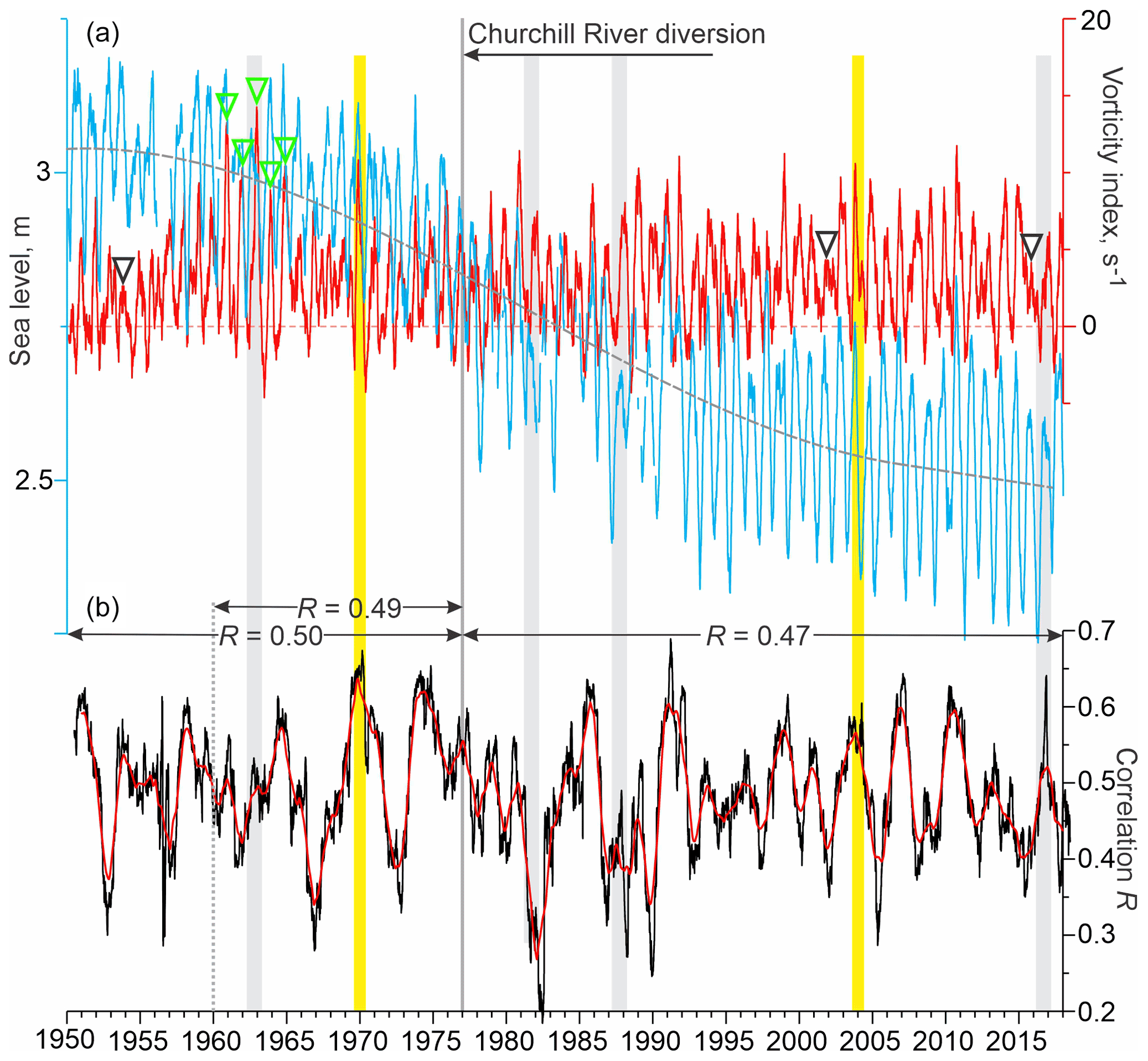
Figure 3(a) 91 d running mean of daily mean atmospheric vorticity index (red, s−1) over Hudson Bay and sea level measured at the tide gauge in Churchill (blue, m). Positive and negative vorticity correspond to cyclonic and anticyclonic atmospheric circulation, respectively. Gray dashed line shows polynomial approximation of the sea-level trend attributed to the glacial isostatic adjustment. Black and green triangles show periods when seasonal vorticity from late fall to early winter was diminished and amplified, respectively. (b) Correlation R between daily vorticity index and sea-level anomaly (SLA) computed for the 365 d moving window (black) with their 365 d running mean (red). All correlations are statistically significant at 99 % confidence. Numbers at the top show correlation between daily vorticity index and SLA computed for 1950–1976 and 1960–1976 and for 1977–2018 pre- and post-diversion, respectively. (a, b) Yellow shading highlights August–May 1969–1970 and 2003–2004, enlarged in Fig. 6. Black arrow indicates onset of the Churchill River diversion. Gray shading highlights periods when the sea-level seasonal cycle was partially disrupted (1981–1982 and 1987–1988), or significantly diminished (1962–1963 and 2016–2017).
Satellite altimetry data from 1993–2020 were used to analyze the relationship between wind forcing and sea-level changes over the entire Hudson Bay. We used the daily fields of absolute dynamic topography (ADT), i.e., the sea surface height (SSH) above geoid, processed and distributed by Copernicus Marine and Environment Monitoring Service (CMEMS; https://marine.copernicus.eu/, last access: 26 August 2021). The ADT is obtained by adding a mean dynamic topography (DT2018, Mulet et al., 2013) to the SLA measured by altimetry satellites. The CMEMS SLA/ADT fields are computed by optimally interpolating data from all satellites available at a given time following a methodology described in Pujol et al. (2016). Prior to mapping, altimetry records are corrected for instrumental noise, orbit determination error, atmospheric refraction, sea state bias, static and dynamic atmospheric pressure effects, and tides. Because in this work we are interested in local (dynamic) changes of sea level, the global mean sea level was subtracted from each ADT map. Then the seasonal climatology was computed for June through August (JJA) and September through November (SON) by averaging all available maps during the respective seasons. Sea ice does not represent a significant problem for computing the climatology, because Hudson Bay is essentially ice-free during these months, especially during SON.
The root-mean-square differences between tide gauge records and collocated SLA/ADT data are usually 3–5 cm (e.g., Volkov et al., 2007; Pascual et al., 2009; Volkov and Pujol, 2012) and do not exceed 10 cm globally (CLS-DOS, 2016). When the altimetry data are averaged to produce the seasonal climatology, the measurement error is greatly reduced (at least by an order of magnitude for 28 years of the altimetry record). It should be noted that altimetry errors near the coast are greater than in the open ocean. This is due to land contamination within the radar footprint and to the fact that the geophysical corrections applied to altimetry data are usually optimized for the open ocean and not for the coastal zones. In classical altimetry products, however, a large percentage of data within 10–15 km from the coast is deemed invalid and not used for generating SLA/ADT maps (e.g., The Climate Change Initiative Coastal Sea Level Team, 2020). Furthermore, satellite altimetry data were used here only for a qualitative assessment of the basin-scale seasonal sea-level patterns in Hudson Bay. Therefore, the reduced quality of altimetry retrievals near the coast is not expected to impact the conclusions of this study.
2.2 River discharge
Churchill River discharge data were obtained from Déry et al. (2016) and extended to 2019; thus, we use a continuous record of daily mean discharge from 1960 to 2019 (Fig. 4a and supplementary material). The record was constructed from gauged observations above Red Head Rapids (station no. 06FD001), which is located ∼87 km from the Churchill River mouth and is the most downstream hydrometric gauge along the Churchill River. When these data were not available, we used upstream gauges (applying a drainage area correction) to fill significant gaps in the time series (see Déry et al., 2005 for detailed methods). Data were adjusted by drainage area (between the hydrometric gauge location and river outlet) and any significant tributary inflows were added to represent discharge at the outlet of the Churchill River.

Figure 4(a) 30 d running mean of the Churchill River discharge (black; 102 m3 s−1) and detrended SLA at Churchill (blue; m). Gray circles show mean discharge pre- and post-diversion with standard deviations depicted with red error bars. (b) Correlation R between daily Churchill River discharge and SLA computed for the 365 d moving window (black) with their 365 d running mean (red). Pink shading highlights statistically insignificant correlations at the 99 % confidence level. Numbers at the top show correlation between daily Churchill River discharge and SLA computed for 1950–1976 and 1977–2018 pre- and post-diversion, respectively. (a, b) Yellow shading highlights August–May 1969–1970 and 2003–2004. Black arrow indicates onset of the Churchill River diversion. Gray shading highlights periods when the sea-level seasonal cycle was partially disrupted (1981–1982 and 1987–1988), or significantly diminished (1962–1963 and 2016–2017).
2.3 Wind forcing
Fields of sea-level pressure (SLP) and 10 m wind velocity at 6 h intervals were derived from the NCEP atmospheric reanalysis (https://psl.noaa.gov/data/composites/hour/, last access: 26 August 2021). We chose the NCEP reanalysis to extend the atmospheric forcing data back to 1950, which covers the tide gauge record from Churchill, while a previous comparison of wind speeds from NCEP and ERA5 (Copernicus Climate Change Service, 2017; Hersbach et al., 2020) with in situ observations from the Churchill weather station revealed an insignificant discrepancy between the two reanalyses and meteorological observations (Dmitrenko et al., 2020). However, we used the ERA5 SLP data to validate atmospheric vorticity derived from NCEP as described below in Sect. 3. For simplicity, cyclones over the Hudson Bay area were manually tracked for August–May 1969–1970 and 2003–2004 using the NCEP SLP fields, with the central position and low SLP tabulated. The horizontal resolution of the NCEP-derived data is 2.5∘ of latitude and longitude.
For the majority of tidal gauge data from the 1950s, sea level at Churchill was recorded hourly. In contrast, the Churchill River discharge from gauged observations above Red Head Rapids (station no. 06FD001) is available daily. The NCEP data on SLP and 10 m wind are available at 6 h intervals. To make these three time series comparable, we analyzed daily means.
For the 1950–2019 and 1960–2019 study periods, a vorticity index was derived from the daily mean SLP NCEP data to characterize the wind forcing and compare it to the time series of sea-level anomalies (Figs. 2a, 3a, and 4a). The vorticity index gives both the sign and magnitude of atmospheric vorticity; it was first proposed by Walsh et al. (1996) and then successfully used for describing atmospheric forcing over the Siberian shelves (Dmitrenko et al., 2008a, b) and Hudson Bay (Dmitrenko et al., 2020). The vorticity index is defined as the numerator of the finite-difference Laplacian of SLP for an area within a radius of 550 km centered at 60∘ N and 85∘ W in Hudson Bay (Fig. 1). A positive index corresponds to cyclonic atmospheric circulation that is typically associated with northerly winds in western Hudson Bay, whereas a negative vorticity index corresponds to anticyclonic atmospheric circulation characterized by southerly winds in western Hudson Bay (Fig. 2). Dmitrenko et al. (2020) examined the spatial uncertainty of atmospheric vorticity estimated at 60∘ N, 85∘ W by computing vorticity for the five-point stencils with a central node shifted relative to 60∘ N, 85∘ W by approximately 280 km northward, eastward, southward, and westward. Their results show that vorticity computed at 60∘ N, 85∘ W best describes major cyclonic storms observed in 2016–2017.
The vorticity index used in this study does not fully explain the observed variability of meridional wind in western Hudson Bay (Fig. 2b), which is mainly responsible for generating storm surges along the coast (Dmitrenko et al., 2020). However, vorticity describes the intensity of cyclonic wind forcing over the entire bay impacting the basin-scale circulation and sea-level deformations along the entire coastline of Hudson Bay (Dmitrenko et al., 2020). Thus, our approach allowed us to extend our findings over the entire bay. We also conducted a validation comparing the NCEP-derived vorticity to that derived from the ERA5 SLP utilizing the Web-Based Reanalysis Intercomparison Tools (https://psl.noaa.gov/cgi-bin/data/testdap/timeseries.pl, last access: 26 August 2021) described by Smith et al. (2014). The comparison showed insignificant differences between the two reanalyses: the NCEP-derived vorticity only slightly exceeds that obtained from ERA5, while the correlation between the NCEP and ERA5-derived vorticities is 0.96 (Fig. 2a).
The Churchill River discharge time series (Fig. 4a) was compiled as follows. First, no significant gaps in the Churchill River discharge record occurred on a daily basis. There were, however, some missing discharge data between 1976 and 1995, with some gaps of up to 3 months (e.g., 1984, 1987). When data gaps occurred, then the upstream hydrometric gauge below Fidler Lake (station no. 06FB001) was used to infill data, with streamflow data adjusted to account for the difference in contributing area between Fidler Lake and the Churchill outlet, following the procedure of Déry et al. (2005). When the upstream hydrometric data were also unavailable, a secondary step was taken to infill data gaps. Missing data on a given day were infilled using the day-of-year mean value of streamflow over the available period of record. This procedure constructed a daily climatology of streamflow (i.e., mean annual hydrograph) based on the availability of data over the period of record.
For the Churchill River, however, we constructed a separate climatology of daily streamflow for the periods prior to and after flow diversion in 1977. Partial diversion began in 1976, allowing less than the full capacity of discharge to be diverted into the Nelson River system, with full operation beginning in 1977. We therefore designated 1977 as the first year when diversion became operational.
It is also important to separate the pre- and post-regulation periods for the analysis of the potential impact natural (pre-diversion) and regulated Churchill River discharge have on sea-level anomalies at Churchill. Déry et al. (2016) reported that the Churchill River diversion caused a significant decline in the mean annual discharge from 37.0±4.2 km3 yr−1 pre-diversion (1964–1973) compared to post-diversion flows (8.4±2.9 and 9.6±4.4 km3 yr−1 for 1984–1993 and 1994–2003, respectively). Déry et al. (2016) further revealed the coefficient of variation (CV) of annual Churchill River discharge increased in inter-decadal CV post-diversion (1984–2013; CV = 0.35–0.67) compared to pre-diversion records (1964–1973; CV = 0.11). Both the decline in mean annual discharge and increase in discharge variability for the post-diversion period necessitate a separate analysis of the impact of river discharge on sea-level variability due to non-stationarity in the discharge record, which was implemented in our analysis.
The sea-level record in Churchill is impacted by the post-glacial isostatic adjustment, with present-day uplift in the Hudson Bay area of ∼10 mm yr−1 (e.g., Sella et al., 2007). Combining satellite altimeter data with the Churchill tide-gauge data gives an uplift rate of about 9.0±0.8 mm yr−1 (Ray, 2015). The crustal uplift is evident in the negative sea-level trend at Churchill of about the same magnitude (Fig. 3a). To examine synoptic to seasonal variability of sea level at Churchill, a polynomial fit was subtracted from the data (Fig. 3a). The polynomial fit better explains long-term variability of sea level at Churchill compared to the linear approximation, with respective coefficients of determination (R2) of 0.41 and 39. Thus, in our study we examined the SLAs against the low-frequency trend conditioned by the post-glacial isostatic adjustment. In addition, the inverse barometer contribution to the water level record was removed using sea-level atmospheric pressure from the NCEP reanalysis. The mean correction attributed to the inverted barometer effect was cm.
We used multiple linear regression to estimate a partial contribution of the cyclonic wind forcing and Churchill River discharge to SLA. In this context, multiple regression uses the least squares method to calculate the value of SLA based on the two independent variables as the vorticity index and Churchill River discharge.
In this section, we examine the impact of wind forcing and local river discharge on sea-level variability at Churchill. We analyze (Sect. 4.1) SLA at Churchill, (Sect. 4.2) atmospheric vorticity over Hudson Bay, (Sect. 4.3) the Churchill River discharge, and (Sect. 4.4) their correlations.
4.1 Sea level
The 30 d running mean of SLA at Churchill ranging from 0.39 m in October 1973 to −0.36 m in April 1981 is dominated by the seasonal cycle (Fig. 4a, blue line). In terms of the long-term monthly mean, sea level shows a seasonal cycle with positive anomalies >0.09 m from September–November and negative anomalies of about −0.14 m from March–April (Fig. 5a).

Figure 5Seasonal cycle of (a) SLA at Churchill (m), (b) atmospheric vorticity over Hudson Bay (s−1), and (c) Churchill River discharge (102 m3 s−1). Seasonal cycle derived using monthly-mean data for (a, b) 1950–2019 (black), (a, b) 1950–1976 (blue), and (c) 1960–1976 (blue) before the Churchill River diversion, and (a, b, c) 1977–2018 (red) after the Churchill River diversion. Error bars show ±1 standard deviation of the mean. (c) Blue and pink dashed lines show the long-term mean discharge before and after diversion, respectively.
There is a substantial difference in the seasonal patterns of sea level between the pre- and post-diversion periods. The long-term variability of sea level (Fig. 3a) and SLA (Fig. 4a) shows no abrupt disruption with the introduction of the Churchill River diversion in 1977. However, the seasonal cycle of SLA generated for pre- and post-diversion shows a characteristic difference in the timing and magnitude of SLA (Fig. 5a). First, for the natural seasonal cycle prior to 1977 (blue line in Fig. 5a), SLA shows two seasonal peaks in June (∼0.04 m; standard error of the mean cm) and November (∼0.11 m, cm). Post-diversion, SLA shows no peak in June, but the magnitude of positive anomalies in September and October increased to >0.08 m. This result is consistent with findings by Gough and Robinson (2000). In contrast to summer, during February–May, the pre- and post-diversion magnitude of SLA decreased and increased, respectively, by m relative to the long-term monthly mean (Fig. 5a). The standard deviation of the monthly mean values is up to 0.1 m (error bars in Fig. 5a). The seasonal pattern of SLA was partially disrupted in 1981–1982 and 1987–1988 and significantly diminished in 1962–1963 and 2016–2017 (Figs. 3a and 4a).
A closer look at the daily data reveals that the sea-level seasonal maximum from October–November is modulated by storm surges frequently observed during the late fall. For example, in 1969–1970 and 2003–2004 (highlighted with yellow shading in Fig. 4), the seasonal cycle of sea level (Fig. 6, thick light blue line) was impacted by synoptic-scale events dominant during October–November (Fig. 6, blue line). These storm surges lasted from ∼3 to 6 d and correspond to positive anomalies of up to 0.5 m in the daily mean sea level (Fig. 6b). In contrast, from December to May, the number and magnitude of storm surges gradually decrease (Fig. 6).
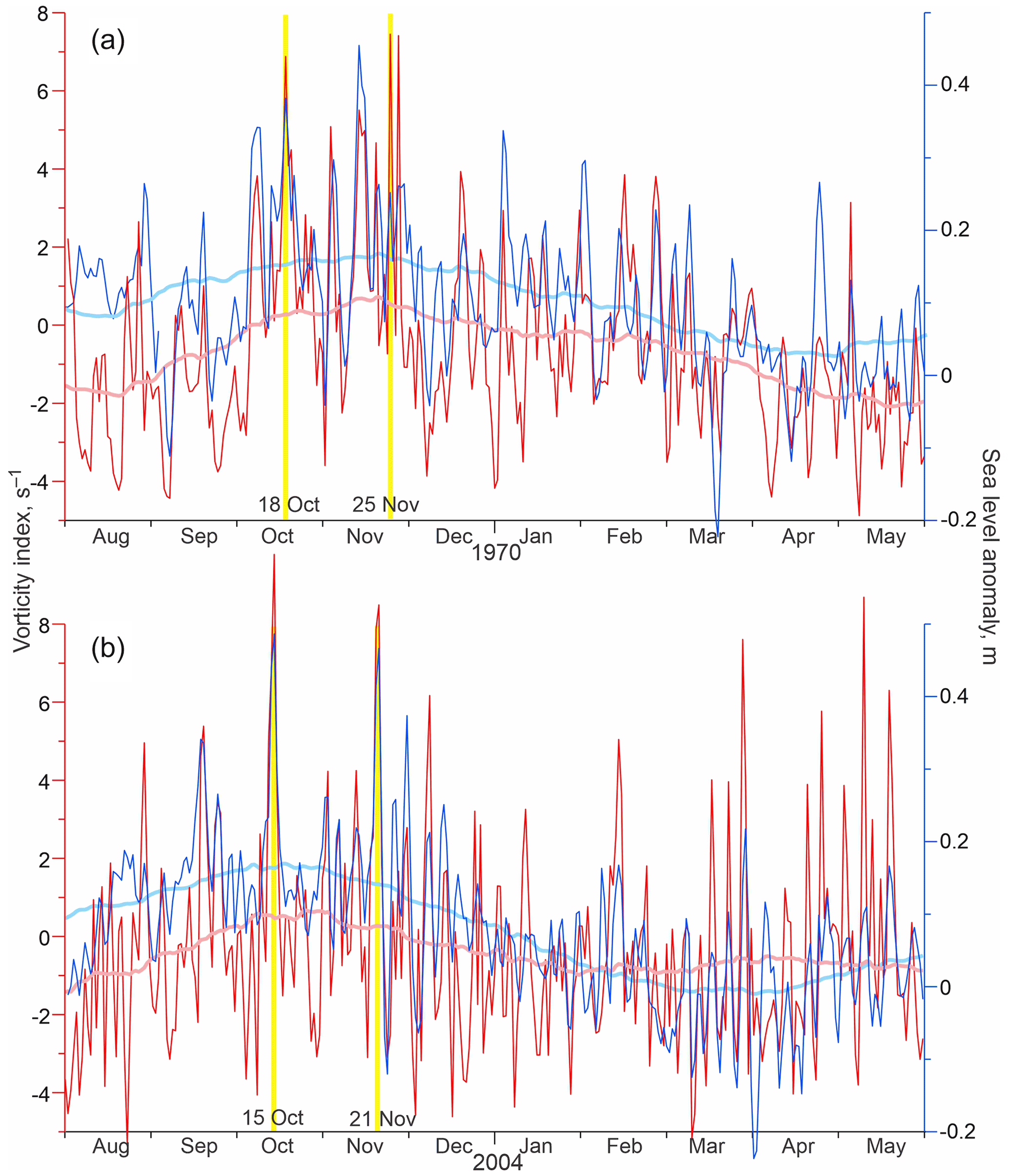
Figure 6Time series of the daily mean vorticity index (red; s−1) and SLA at Churchill (blue; m) with their 91 d running mean in pink and light blue, respectively, for August–May (a) 1969–1970 and (b) 2003–2004. (a, b) Vertical yellow lines highlight coherent peaks in vorticity and sea level in October and November.
4.2 Wind forcing
The vorticity index shows predominant cyclonic atmospheric circulation over Hudson Bay (mostly positive values in Fig. 3a, red line), which agrees with results presented by Saucier et al. (2004) and St-Laurent et al. (2011). The strongest positive (cyclonic) vorticity is observed from fall 1962 to winter 1963 (vorticity index exceeded 14 s−1), while the strongest negative (anticyclonic) atmospheric forcing (vorticity < 4 s−1) is recorded during summer 1963 (Fig. 3a). Overall, the alternation between monthly mean cyclonic and anticyclonic wind forcing is mostly governed by the seasonal cycle in vorticity (Fig. 5b). The monthly mean vorticity increases from 4 s−1 in September to ∼8 s−1 in November and then gradually returns to ∼4 s−1 in February (Fig. 5b). During March–May and August, vorticity is relatively low (<2 s−1), and only in June and July does vorticity change to weak anticyclonic (slightly negative) values (Fig. 5b). The seasonal cycle in atmospheric vorticity shows an insignificant difference pre- and post-diversion. From May to August and in December, there is no difference between the long-term monthly mean and monthly mean estimates for pre- and post-diversion (Fig. 5b). For other months, the difference does not exceed ±0.7 s−1.
The interannual variability of wind forcing is mainly attributed to year-to-year changes in the cyclonic atmospheric circulation during fall–winter months. The seasonal amplitude of vorticity is significantly diminished in 1953–1954, 2001–2002, and 2015–2016 when the seasonal mean vorticity index for late fall to the beginning of winter did not exceed 8 s−1 (black triangles in Fig. 3a). In contrast, during 1960–1965, the vorticity seasonal cycle is amplified with the seasonal mean vorticity index between late fall and early winter up to 28 s−1 (green triangles in Fig. 3a). The standard deviation of the monthly mean vorticity shown by error bars in Fig. 5b gradually decreases from ±4.5 s−1 in December to ±2.8 s−1 in March–April.
Analysis of the daily vorticity time series sheds light on the origin of seasonality in vorticity. Positive seasonal anomalies from September–December (Figs. 3a and 5b) are partly attributed to the occurrence of numerous vorticity peaks. For example, in 1969–1970 and 2003–2004 (highlighted with yellow shading in Fig. 3), the seasonal enhancement of atmospheric vorticity (Fig. 6, thick pink line) was partially conditioned by synoptic-scale events recorded during October–November 1969 and 2003 (Fig. 6, red line). The strongest vorticity peaks were observed on 18 October and 25 November 1969 (>4 s−1; Fig. 6a) and 15 October and 21 November 2003 (> 5 s−1; Fig. 6b). The SLP spatial distribution reveals that each of these peaks is attributable to a cyclone passing over Hudson Bay, with the center of low SLP located over the central Hudson Bay on 18 October and 25 November 1969 (Fig. 7a and b, respectively) and 15 October and 21 November 2003 (Fig. 7c and d, respectively). The horizontal gradients of SLP over western Hudson Bay ranged from 0.020 hPa km−1 (25 November 1969; Fig. 7b) to 0.035 hPa km−1 (21 November 2003; Fig. 7d). Overall, from 1 September to 31 December, vorticity exceeded 2 s−1 9 and 12 times in 1969 and 2003, respectively. In contrast, from 1 January to 30 April 1970 and 2004, vorticity exceeded 2 s−1 only four and seven times, respectively (Fig. 6). This suggests that the seasonal cycle in atmospheric vorticity is partially governed by the number and strength of cyclones passing over Hudson Bay.

Figure 7Sea-level atmospheric pressure (hPa) for coherent peaks in atmospheric vorticity and sea level at Churchill, highlighted in Fig. 6 with yellow lines: (a) 18 October 1969, (b) 25 November 1969, (c) 15 October 2003, and (d) 21 November 2003.
4.3 Local river discharge
The time series of Churchill River discharge (Fig. 4a) is dominated by (i) the introduction of the flow diversion in 1977 and (ii) the seasonal hydrologic cycle. The mean discharge dropped by about one-third from 1190 m3 s−1 (1960–1976) to about 400 m3 s−1 following the diversion in 1977. At the same time, the standard deviation of the mean discharge increased from about ±300 to ±470 m3 s−1 following the diversion (Fig. 4a). This is in line with results by Déry et al. (2016). The mean annual timing of maximum river discharge during late spring to summer is not significantly disrupted by the diversion (Fig. 5c). The magnitude of the monthly mean discharge pre- to post-diversion, however, reduces from about 5-fold in March to about 2.5-fold in May–August (Fig. 5c). After diversion, the standard deviation of the monthly mean discharge doubles from May to October (Fig. 5c). In contrast, from December to April, the standard deviation of the monthly mean was not significantly impacted by the diversion (Fig. 5c).
4.4 Sea-level response to wind forcing and local river discharge
Our data show that SLA in Churchill, atmospheric vorticity over Hudson Bay, and Churchill River discharge all show variability dominated by the seasonal cycle (Figs. 3a, 4a, and 5). In what follows, SLA at Churchill is first compared to the atmospheric vorticity, and then to the Churchill River discharge, with the main focus on the seasonal cycle.
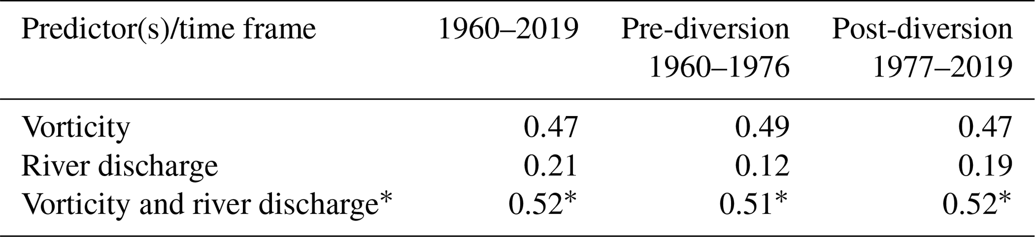
The correlation between the daily vorticity index and SLA from 1950–2019 and 1960–2019 is 0.48 and 0.47, respectively, with insignificant differences between correlations estimated for periods pre- and post-diversion (0.49 and 0.47, respectively; Fig. 3b and Table 1). For the ice-free period from June to November, correlations for whole period and pre- and post-diversion increase to 0.54, 0.52 and 0.55 (Table 2), respectively, compared to 0.47, 0.49 and 0.47 for the ice-covered period from December to May (Table 3). We test the difference between correlations estimated for the ice-covered and ice-free seasons using the Fisher z transformation (Fisher, 1921). Statistical assessment shows that the only differences between correlations estimated for whole period and post-diversion are statistically significant at the 99 % confidence level.
Table 1Correlations (R) of daily atmospheric vorticity and/or Churchill River discharge against sea-level anomalies in western Hudson Bay for the whole annual cycle.
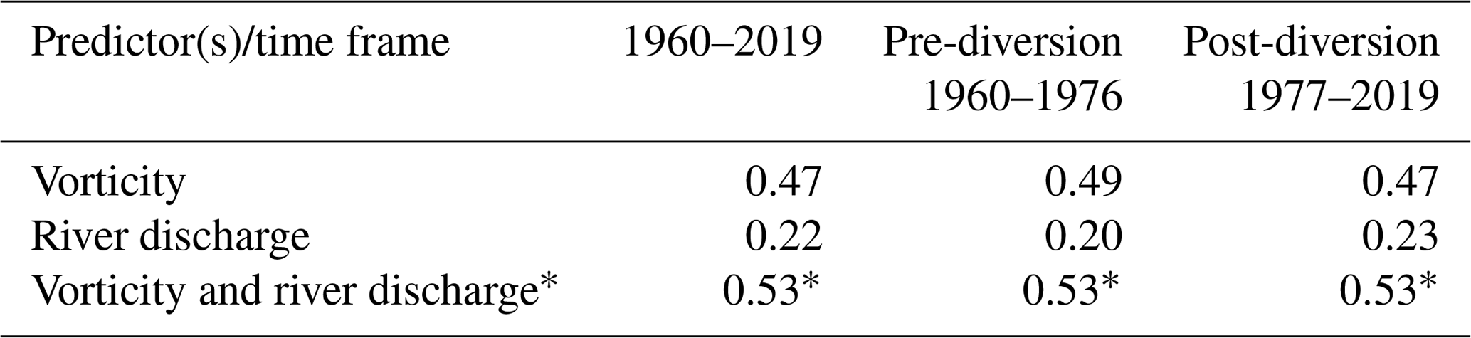
* The coefficient of multiple correlation is estimated based on the multiple linear regression analysis.
Table 2Correlations (R) of monthly-mean atmospheric vorticity and/or Churchill River discharge against sea-level anomalies in western Hudson Bay for the ice-free period (June–November).
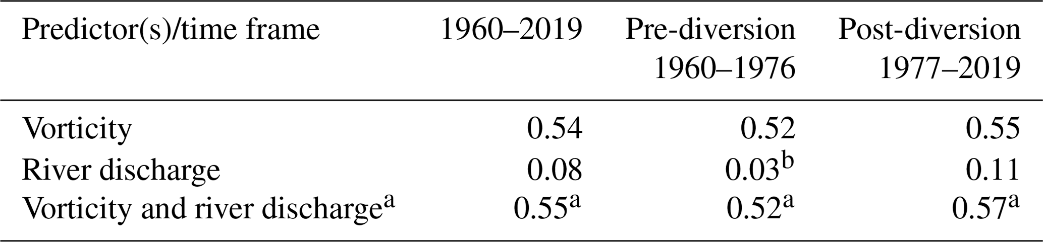
a The coefficient of multiple correlation is estimated based on the multiple linear regression analysis. b Correlation not statistically significant at the 99 % confidence level.
The relationship between vorticity and SLA changes significantly from one year to another. The mean annual correlations in Fig. 3b show these differences ranging from 0.18 in 1982 to 0.69 in 1991. During periods when the sea-level seasonal cycle almost disappears (1981–1982 and 1987–1988), the mean annual correlation drops to about 0.3 and 0.4, respectively (Fig. 3b). When the sea-level seasonal cycle is diminished (1962–1963 and 2016–2017), a modest correlation of ∼0.5 is estimated (Fig. 3b). For time periods enlarged in Fig. 6, the annual mean correlation significantly exceeds the long-term mean of 0.47, attaining 0.65 and 0.57 for 1969–1970 and 2004–2005, respectively (Fig. 3b). The direct linkage between vorticity and SLA is evident in Fig. 6. During September–November 1969 and 2003, all significant synoptic peaks in SLA are consistent with those in atmospheric vorticity, including storm surges on 18 October and 25 November 1969 (Fig. 6a) and on 15 October and 21 November 2003 (Fig. 6b).
In contrast to atmospheric vorticity, the correlation between daily SLA and river discharge is significantly smaller. Through the full record from 1960 to 2019, the correlation is 0.22, with an insignificant difference between pre- and post-diversion (0.20 and 0.23, respectively; Fig. 4b and Table 1). For the ice-free period from June to November, correlations drop close to or below the level of statistically significant values for the whole and pre-diversion periods (0.08 and 0.03, respectively), and to 0.11 post-diversion (Table 2) compared to 0.21, 0.12, and 0.19 for the ice-covered period from December to May (Table 3). Note that the difference between correlations estimated for the ice-covered and ice-free seasons is statistically significant for only 1960–2019.
Table 3Correlations (R) of monthly-mean atmospheric vorticity and/or Churchill River discharge against sea-level anomalies in western Hudson Bay for the ice-covered period (December–May).
* The coefficient of multiple correlation is estimated based on the multiple linear regression analysis.
Similar to the linkage between vorticity and SLA, the relationship between river discharge and SLA shows significant interannual variability. Correlations computed through the 365 d moving window show negative to positive values ranging from −0.3 to 0.7 with about 15 % of estimates below the level of statistical significance (Fig. 4b). Among all events when the amplitude of the sea-level seasonal cycle was strongly reduced, only 1962–1963 and 1981–1982 show statistically significant correlation between river discharge and SLA of ∼0.25 (Fig. 4b). For events in 1987–1988 and 2016–2017, correlation is relatively close to or below the level of statistical significance (Fig. 4b). The interannual difference in contribution of river discharge to the sea-level variability is also evident for 1969–1970 and 2004–2005. In 1969–1970, the annual mean correlation shows relatively modest contributions of river discharge to sea-level variability (correlation R∼0.29; Fig. 4b) as compared to correlation with atmospheric vorticity (R∼0.65; Fig. 3b). In 2004–2005, however, there is no correlation between SLA and river discharge (Fig. 4b), and sea-level variability is impacted by wind forcing (R=0.57; Fig. 3b).
Overall, our results show that the wind forcing impacts the synoptic and seasonal variability of sea level. In what follows, we use the coefficient of determination (R2, where R is correlation coefficient in Tables 1–3) to describe the proportion of the variance in sea level that is explained by the wind forcing, river discharge, and the wind forcing and river discharge together. Through the whole annual cycle from 1960 to 2019, wind forcing explains about 22 % of sea-level variability, while river discharge contributes only ∼5 %. Multiple regression analysis shows that on average, both explain ∼28 % of sea-level variability (Table 1).
Our results also reveal the important role of sea-ice cover and river diversion in modifying controls on sea-level variability. During the ice-free seasons from 1960–1976, the contribution of wind forcing is 27 %, and the role of river discharge is negligible (Table 2). Post-diversion, cyclonic wind forcing and river discharge contribute 30 % and 1 %, respectively. Together they explain up to 32 % of sea-level variability (Table 2). During the ice-covered season, the contribution of vorticity is reduced to 22 %, with insignificant differences between pre- and post-diversion (Table 3). The contribution of river discharge varies from 1 % for pre-diversion to 4 % for post-diversion. Wind and river forcing together explain ∼27 % of sea-level variability for both pre- and post-diversion periods (Table 3). Summarizing these results, we point out that the sea-ice cover reduces the influence of wind forcing, and the influence of local river discharge is slightly increased primarily during the ice-covered post-diversion period. Post-diversion, the magnitude of river discharge was reduced about 3-fold, but seasonal variability increased by a factor of 1.5 (Fig. 4a and Déry et al., 2016). Thus, we attribute the increase in river discharge forcing during the post-diversion period mainly to the higher variability in river discharge from May to November (Figs. 4a, 5c, and Déry et al., 2016). Note that during May about 85 % of Hudson Bay is ice covered (Tivy et al., 2011), and the standard deviation of the monthly mean discharge in May increases from about ±170 pre-diversion to ±380 m3 s−1 post-diversion.
Our results show that sea-level variability at Churchill is rather influenced by wind forcing, with discharge from the Churchill River playing a secondary role. Overall, the atmospheric vorticity explains up to 30 % of sea-level variability at Churchill, with local river discharge contributing up to only 5 % (Tables 1–3). This suggests that in western Hudson Bay the northerly winds associated with cyclonic wind forcing (Fig. 2b) generate storm surges along the coast due to a surface Ekman on-shore transport. This is consistent with results from Dmitrenko et al. (2020), who used mooring records and Churchill tide gauge observations in 2016–2017 to identify this mechanism. A direct response of the water level to balance wind stress acting on the surface does not play a role for generating SLA because there is no correlation between SLA and zonal wind (not shown).
The SLA seasonal cycle in Fig. 5a is only partially explained by seasonality in wind forcing and local river discharge. The SLA seasonal cycle is also consistent with summertime warming and freshening, and wintertime cooling and salinification. During the ice-free summer period, the water column warms, and seawater becomes less dense and expands, causing the thermosteric sea-level rise. In addition, during summer, riverine water and sea-ice meltwater decrease salinity of the bay, thus causing the halosteric sea-level rise. It seems that these factors can explain the significant fraction of the SLA seasonal variability that is not explained by wind forcing and local river discharge. However, the detailed assessment of the thermosteric and halosteric contributions to the Hudson Bay sea-level variability is beyond the scope of this paper. In this context, we point out that we examine only the direct impact of the river discharge on the sea level in the Churchill River mouth, ignoring the cumulative effect of riverine water on steric height. This simplification seems to be reasonable because the residence time of the riverine water fraction in southwestern Hudson Bay during summer is ∼1–3 months (Granskog et al., 2009).
For the seasonal timescales, increased cyclonic activity during fall to early winter impacts the seasonal cycle in SLA. In contrast to Gough and Robinson (2000), we assert that a positive SLA from September–November (Fig. 5a) is attributed to enhanced atmospheric vorticity rather than to the local river discharge. The signature of the local river discharge is, however, traceable through the SLA seasonal cycle. During the pre-diversion period, positive SLA in June (Fig. 5a) appears to be linked to the spring freshet of the Churchill River (Fig. 5a and c). However, post-diversion this positive SLA in June vanishes due to the abrupt decrease in the Churchill River discharge during the spring freshet from ∼ 1500 to 700 m3 s−1 (Fig. 5c). Gradual decreases in Churchill River discharge from June and July to April for both pre- and post-diversion cannot explain the positive SLA from fall to winter, especially during the post-diversion period when the mean annual Churchill River discharge decreases to ∼400 m3 s−1 (Fig. 5c). Note that the cumulative effect of riverine water on steric height is neglected.
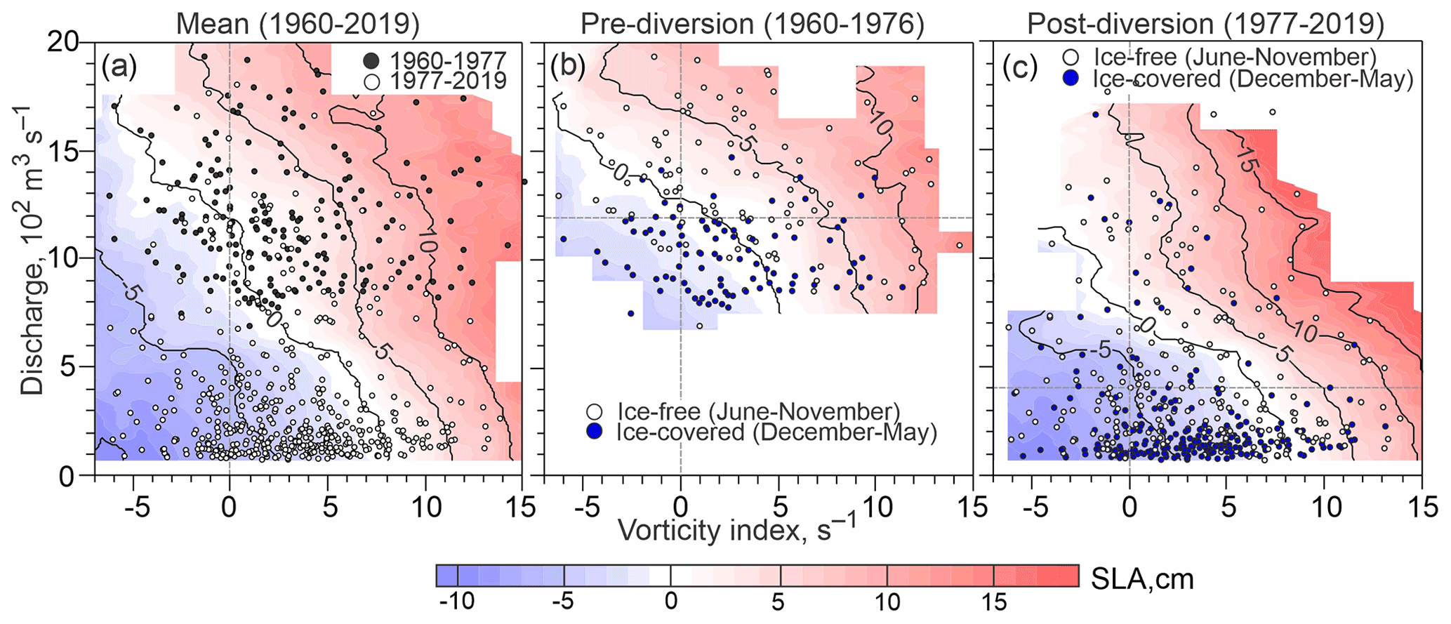
Figure 8Colour shading shows monthly mean sea-level anomalies (cm) from tidal gauge at Churchill versus atmospheric vorticity (s−1; horizontal axis) and Churchill River discharge (102 m3 s−1; vertical axis) for (a) entire period of river discharge observations (1960–2019), and (b) before and (c) after the Churchill River diversion in 1977. Scatter plots show monthly mean vorticity and river discharge for (a) 1960–1976 (black circles) and 1977–2019 (white circles), and (b, c) ice-free season (June–November; white circles) and ice-covered season (December–May; blue circles). Horizontal gray dashed line shows mean river discharge (c) before and (d) after diversion.
An additional perspective on SLA response to atmospheric and river forcing comes from a comparison of the monthly mean vorticity and Churchill River discharge time series with SLA at Churchill for the whole period of river discharge observations, and the pre- and post-diversion periods (Fig. 8a, b, and c, respectively). The SLA patterns for the whole period of river discharge observation (Fig. 8a) are strongly impacted by changes in the magnitude of discharge during the pre- and post-diversion periods, as previously discussed. In contrast, the SLA patterns compiled for the pre- and post-diversion periods (Fig. 8b and c, respectively) provide more precise features of the SLA response to atmospheric and river forcing. In general, comparing atmospheric vorticity to sea level at Churchill shows that cyclones generate positive SLA up to 0.15 m (Fig. 8c). The maximum SLA response to cyclonic atmospheric forcing is observed during the ice-free period (pink shading and white circles in Fig. 8b and c), which is consistent with results of the correlation analysis (Tables 2 and 3). The combination of anticyclonic (negative) vorticity and low river discharge generates negative SLA up to 0.09 m during both ice-free and ice-covered seasons (blue shading in Fig. 8b and c).
The zero SLA contour in Fig. 8b and c is displaced relative to the zero vorticity and the long-term mean river discharge for the pre- and post-diversion periods. This indicates that these two predictors alone are insufficient to entirely explain the sea-level variability, and that there must be other contributing factors. Correlation analysis (Tables 2 and 3) suggests that sea ice also plays a role in modifying the impact of atmospheric forcing on SLA. In this context, Fig. 8 reveals the role of sea-ice cover for generating the SLA. The sea level at Churchill exhibits negative SLA while atmospheric vorticity is positive, but not exceeding ∼6–8 s−1 (Fig. 8). This situation is usually observed during the ice-covered season when river discharge is below the annual mean (blue circles and blue shading in Fig. 8b and c). We attribute this disruption to the sea-ice cover. Throughout the entire year, positive SLA is generated in response to strong cyclones with vorticity exceeding ∼6–8 s−1 regardless of the river discharge contribution and sea-ice conditions (red shading in Fig. 8 for vorticity –8 s−1). During the ice-covered season, at relatively low river discharge (< 1200 and 350 m3 s−1 for pre- and post-diversion, respectively), negative SLA is associated with positive vorticity <6–8 s−1 (blue circles and blue shading in Fig. 8b and c). Thus, vorticity ∼6–8 s−1 is suggested to be a very rough estimate of the vorticity threshold attributed to the sea-ice impact. Above this threshold, sea ice does not eliminate wind stress from the water column, and wind forcing impacts sea-level variability in Churchill year-round. Below this threshold, sea ice eliminates wind forcing and a negative SLA is conditioned by low river discharge. In fact, extension of the landfast ice as well as sea-ice roughness and concentration can play a role in modifying the thresholds at which wind impacts the SLA. When the Churchill River discharge exceeds the monthly means of 1500–1600 and ∼900 m3 s−1 for pre- and post-diversion periods, respectively, positive SLA results regardless of wind forcing.
Our results on the mechanisms of sea-level variability at Churchill differ from those obtained by Gough and Robinson (2000). First, using sea-level and river discharge data from 1974–1994, they found that correlation between Churchill River discharge and SLA in Churchill explains 43 % of sea-level variability (versus the 5 % derived in our analysis). Second, Gough and Robinson (2000) explain a positive SLA observed in Churchill from October–November by the river discharge pulse into the James Bay region with an advective lag of ∼4–5 months. Furthermore, Gough et al. (2005) speculate that positive SLA during fall is attributed to the James Bay riverine water fraction, which does not exit the bay through Hudson Strait but instead re-circulates in western Hudson Bay. The halosteric sea-level changes associated with this freshwater fraction are suggested to generate a positive SLA observed in Churchill from October–November. The pathway of this water and the reason for disrupting the mean cyclonic circulation in the bay were, however, specified in neither Gough and Robinson (2000) nor Gough et al. (2005). The distance from James Bay to Churchill measured along the coast is roughly 1000 km. For a 120–150 d lag between peaks in river discharge to James Bay in June (Déry et al., 2005) and maximum positive SLA at Churchill in November, this distance suggests the unrealistic rate of mean advective velocity to be ∼8–10 cm s−1. Note that Dmitrenko et al. (2020) estimated the velocity of the northward flow along the western coast of Hudson Bay during strong cyclonic storms to be ∼13 cm s−1, which significantly exceeds the annual mean meridional transport of ∼1–2 cm s−1.
Overall, the hypothesis by Gough and Robinson (2000) and Gough et al. (2005) about the linkage between the river discharge pulse into James Bay and a positive SLA in Churchill is suggestive of the seasonal disruption of the Hudson Bay cyclonic circulation that is in line with the seasonal pattern of atmospheric vorticity in Fig. 5b. Based on satellite altimetry and numerical simulation, Ridenour et al. (2019a) revealed a seasonal reversal to anticyclonic circulation in southwestern Hudson Bay from May–July, with a return to strong cyclonic circulation in fall in response to the seasonal patterns of surface stress. This is consistent with the seasonal cycles of vorticity presented in Fig. 5b. However, among ∼120–150 d of the hypothetical transit time from James Bay to Churchill, the anticyclonic atmospheric forcing is persistently observed only during May–July; in August, vorticity returns to cyclonic (Fig. 5b). In the 3 months before the occurrence of the positive SLA at Churchill in November, the atmospheric forcing has already retuned to cyclonic (Fig. 5b). In this context, the hypothesis by Gough and Robinson (2000) and Gough et al. (2005) linking SLA in Churchill to river discharge in James Bay seems to be inconsistent. In what follows, we provide additional arguments to support our finding on the role of wind forcing in generating the SLA at Churchill.
First, Tushingham (1992) provides the time series of sea level at Churchill and the Churchill River discharge from 1972 to 1989 (Fig. 5 from Tushingham, 1992). These time series clearly show an overall low positive correlation completely disrupted in 1973–1974, 1977, and 1987–1986, which is consistent with our analysis (Fig. 4). For 1973–1974 and 1987–1986, the annual-mean correlation was estimated to be about −0.1 and is below the level of statistical significance (Fig. 4b). Overall, from 1960 to 2019, there were 19 events that lasted up to 1.8 years in duration when correlations between the SLA and river discharge were statistically insignificant or even negative (Fig. 4b). This calls into question the correlations between Churchill River discharge and SLA in Churchill reported by Gough and Robinson (2000) and Gough et al. (2005). Note that the period from 1972 to 1989 used by Tushingham (1992) overlaps with the majority of the period from 1974 to 1994 used by Gough and Robinson (2000).
Second, Ward et al. (2018) analyzed daily data from the Global Runoff Data Centre for 187 stations including Churchill and daily-maximum sea-level data from the Global Extreme Sea-level Analysis. They found no statistically significant dependence between annual maxima of the Churchill River discharge and sea level. For comparison, along the Pacific coast of North America, the correlation ranged from 0.2 to 0.4 and accounted for 4 %–16 % of the variation in sea level. This is consistent with a previous concern about the significant impact of Churchill River discharge on SLA in Churchill.
Third, our analysis shows that the seasonal cycle in sea-level variability with positive SLA during fall is observed not only in Churchill, but also along the eastern coast of Hudson Bay in Inukjuak (Figs. 1 and 9). While the sea level record at Inukjuak is short and not continuous, a positive SLA is recognizable during fall 1969–1970 and 1973–1976 (Fig. 9, blue line). Note that the seasonal SLA at Inukjuak cannot be generated locally because the annual mean (1964–2000) discharge of the local Innuksuak River is only 3.3 km3 yr−1, about 3 times smaller than the Churchill River discharge post-diversion (Godin et al., 2017). In contrast, the seasonal pattern in SLA at Inukjuak is generated by the same cyclonic forcing as in Churchill. Seasonal SLA in Inukjuak is consistent with seasonal amplification of atmospheric vorticity (Figs. 5b and 9). Moreover, in Inukjuak, the sea-level peaks on 18 October and 25 November 1969 are coherent with peaks in atmospheric vorticity (Fig. 9) and sea level at Churchill (Fig. 6a). From the preceding analysis we explicitly know that these two vorticity peaks were generated by cyclones passing over the bay (Fig. 7a). The coherent peaks in sea level in Churchill and Inukjuak suggest that cyclones that were centered over Hudson Bay on 18 October and 25 November 1969 generated storm surges on both the eastern and western coasts of Hudson Bay. This is also supported by a coherent response of sea level to atmospheric forcing at Cape Jones Island and North Kopak Island (Figs. 1 and 9). Our hypothesis is also consistent with results of sea-level numerical simulations in response to cyclones passing over the bay in 2016–2017 (Dmitrenko et al., 2020). For synoptic storm surges, on-shore Ekman transport increases the mass of water column along the coast (the barotropic component). The seasonal baroclinic component appears during summer when water is fresher and warmer causing the thermosteric and halosteric sea-level rise along the coast.
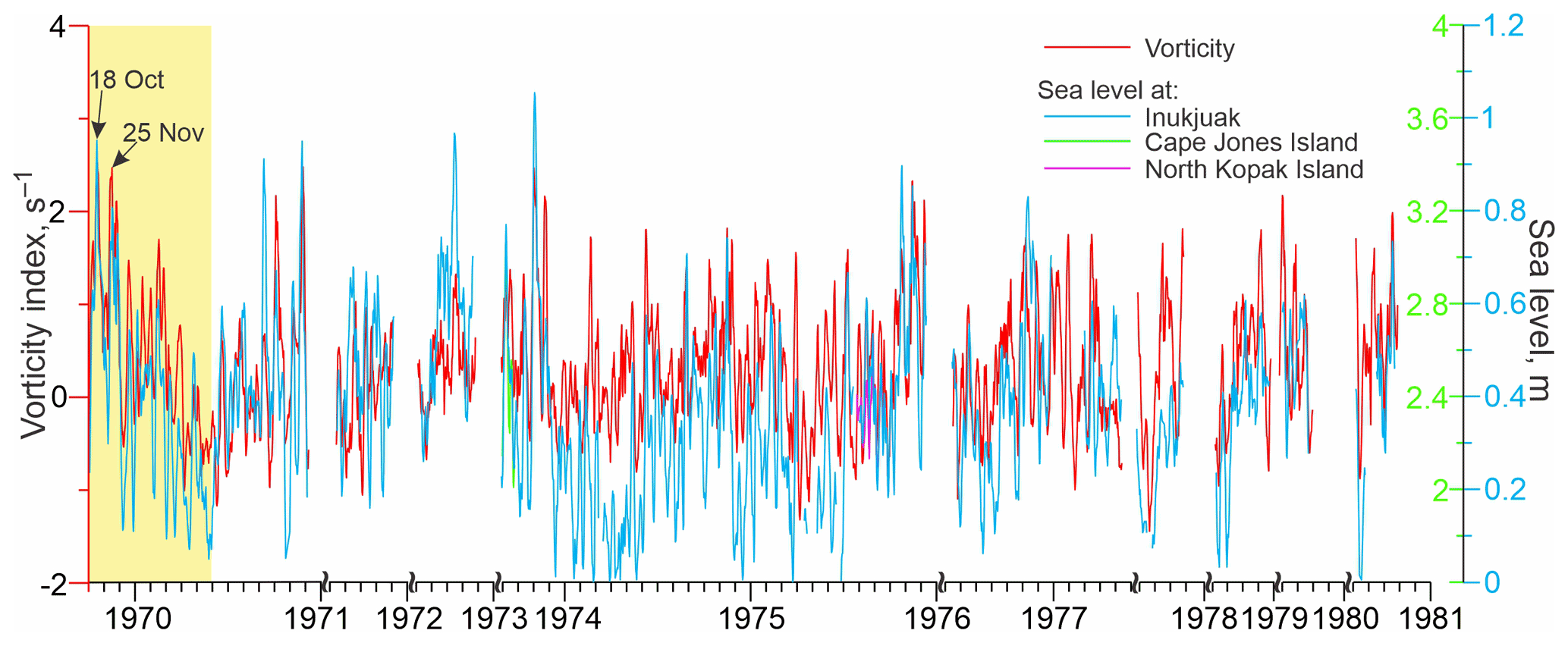
Figure 9Time series of 7 d running mean for daily atmospheric vorticity index (red, s−1) over Hudson Bay and daily mean sea level (m) measured at the tide gauge in Inukjuak (blue), Cape Jones Island (green), and North Kopak Island (purple). Yellow shading highlights October–May 1969–70. Black arrows indicate two cyclonic storms in 18 October and 25 November 1969 with atmospheric forcing shown in Fig. 7a and b, respectively. Right vertical axis shows sea-level scale for Inukjuak (blue), Cape Jones Island, and North Kopak Island (green).
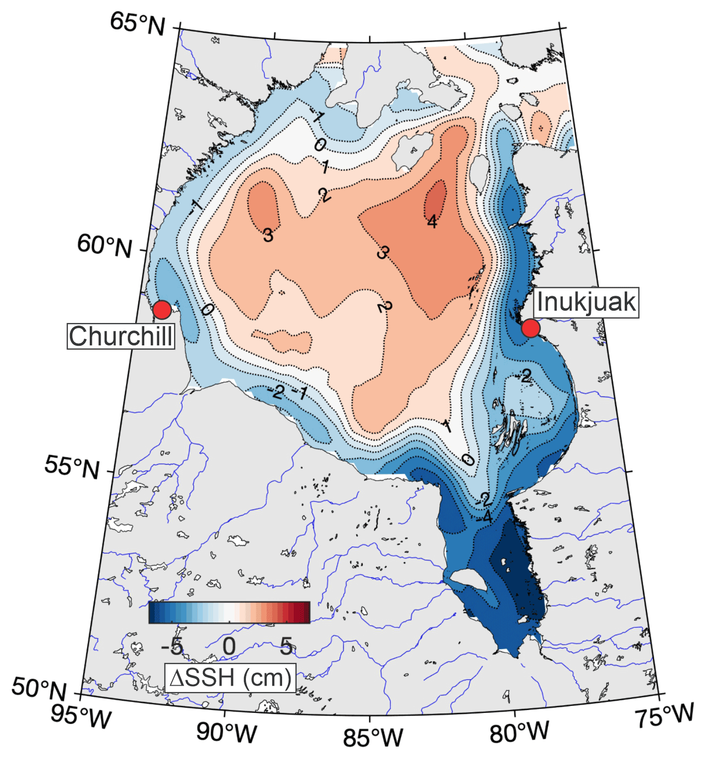
Figure 10The long-term mean (1993–2020) difference between sea surface height (SSH; cm) in summer (June–August) and fall (September–November) derived from the satellite altimetry. Red dots depict the tide gauge in Churchill and Inukjuak.
Fourth, satellite altimetry reveals a spatially uniform response of sea level to the seasonal cycle in atmospheric vorticity along the whole coast of Hudson Bay (Fig. 10). For 1993–2020, we examine the difference between the sea surface heights (SSHs) during summer, when monthly mean atmospheric vorticity changes from −0.7 s−1 in June to 1.1 s−1 in August, and fall, when vorticity increases from 4.2 s−1 in September to 7.3 s−1 in November (Fig. 5b). Results suggest that enhanced cyclonic vorticity during fall generates seasonal SSH elevation over the entire coast of Hudson Bay with SSH differences between fall and summer ranging from > 5 cm in James Bay to ∼1 cm along the northwest coast (Fig. 10). This confirms our results that a positive SLA during fall is generated over the entire coast of Hudson Bay, and particularly in Churchill and Inukjuak, in response to enhanced cyclonic wind forcing (Figs. 5a, b, and 9). Overall, our third and fourth points suggest that the hypothesis of Gough and Robinson (2000) and Gough et al. (2005) about a linkage between river discharge into James Bay and SLA in Churchill is inconsistent.
One may suggest that seasonal SSH elevation in Fig. 10 can be partly due to the thermosteric and halosteric sea-level rise. During summer, the Hudson Bay coastal domain receives a large amount of fresh and warm water from river runoff. The seasonal tendency for river discharge, however, is opposite to that for the SSH in Fig. 10. For 1988–2000, Déry et al. (2005) reported that the total discharge of rivers flowing into Hudson Bay peaks in June at ∼3.6 km3 d−1, which significantly exceeds the secondary maximum in October (∼2.3 km3 d−1). The seasonal mean total river discharge in September–November (∼1.9 km3 d−1) is 1.5 times smaller compared to ∼2.8 km3 d−1 in June–August. Based on these estimates, the river discharge seasonal cycle in June–November is inconsistent with that for the SSH in Fig. 10. The cumulative effect of river discharge on the seasonal cycle can play a role, but the residence time of the riverine water fraction in southwestern Hudson Bay during summer is relatively small (∼1–3 months; Granskog et al., 2009).
Finally, our results on the atmospheric forcing of the Hudson Bay SLA are in agreement with conclusions by Piecuch and Ponte (2014, 2015). Using ocean mass measurements from satellite gravimetry conducted during the Gravity Recovery and Climate Experiment, they found that wind forcing dominates sea-level and mass variability in Hudson Bay, and wind might drive Hudson Bay mass changes due to wind-driven outflow through Hudson Strait (Piecuch and Ponte; 2014). For the sea-level interannual variability in Hudson Bay, also evident in Fig. 4a, Piecuch and Ponte (2015) revealed a wind-driven barotropic fluctuation that explains most of the non-seasonal sea-level variance. Furthermore, they suggest that anomalous inflow and outflow through Hudson Strait, which impacts sea-level variability in Hudson Bay, are driven by wind stress over Hudson Strait. This highlights the role of wind forcing in amplifying the freshwater outflow from Hudson Bay, as also suggested by Straneo and Saucier (2008) and Dmitrenko et al. (2020).
In summary, we suggest that seasonal amplification of atmospheric vorticity, partially conditioned by the number and strength of cyclones passing over the bay during fall to early winter, generates the seasonal cycle in sea-level variability over the entire bay as depicted schematically in Fig. 11. Cyclones passing over Hudson Bay during fall to early winter cause on-shore Ekman transport and storm surges over the entire coast of Hudson Bay (Fig. 11a). In summer, anticyclonic wind forces off-shore Ekman transport, lowering sea level along the coastline of Hudson Bay (Fig. 11b).
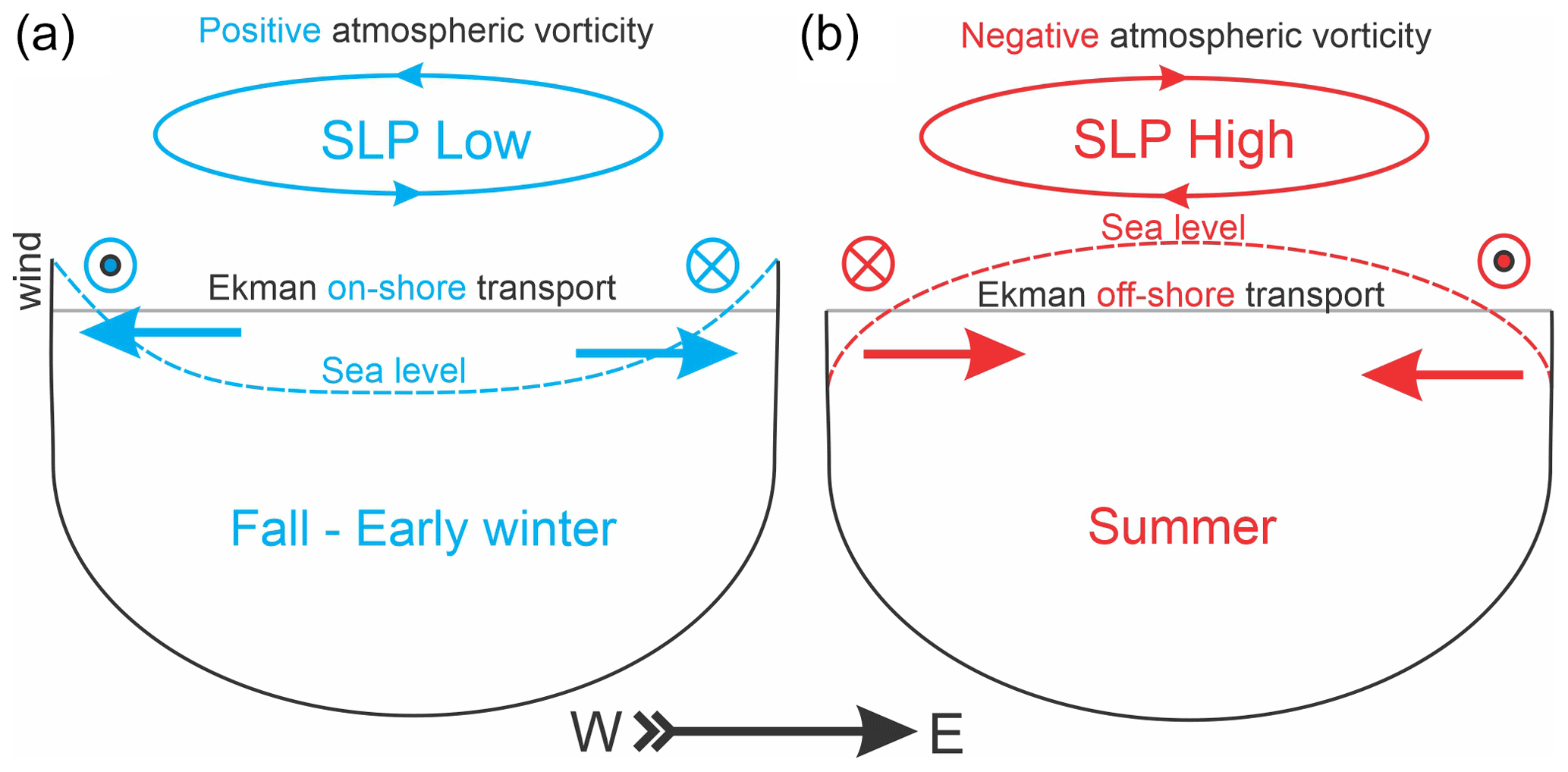
Figure 11Diagram of the proposed impact of the seasonal changes in atmospheric vorticity on the sea-level seasonal variability in Hudson Bay. (a) Positive (cyclonic) vorticity during October–December causes onshore Ekman transport and storm surges over the coast. (b) Negative (anticyclonic) vorticity during June–July forces offshore Ekman transport. During winter, a complete sea-ice cover reduces momentum transfer from wind stress to the water column diminishing impact of atmospheric forcing on sea-level variability. Dotted and crossed circles depict northerly and southerly along-shore surface winds, respectively.
Our analysis revealed that in contrast to previous research, the local Churchill River discharge explains only up to 5 % of the sea-level variability at Churchill. Cyclonic atmospheric forcing is shown to explain from 22 % during the ice-covered winter–spring season to 30 % during the ice-free summer–fall season (Tables 1–3). Multiple regression analysis showed that atmospheric forcing and local river discharge together can explain up to 32 % of the sea-level variability at Churchill. We found that a positive sea-level anomaly in Churchill during fall is partially conditioned by the seasonal cycle in atmospheric vorticity, with prevailing cyclonic wind forcing during fall to the beginning of winter (Fig. 5). Sea-ice cover reduces wind stress on the water column during the ice-covered season from December to May, and cyclonic wind forcing generates positive sea-level anomalies at Churchill when only the monthly mean vorticity exceeds ∼6–8 s−1 (Fig. 8). In this context, transition towards a longer open water season (e.g., Hochheim and Barber, 2014) is expected to increase the contribution of atmospheric forcing to sea-level variability.
We expanded our observations at Churchill to the bay-wide scale using sea-level observations along the eastern coast of the bay and satellite altimetry. A coherent sea-level response to atmospheric forcing observed at the opposite sides of Hudson Bay suggests that the spatial scale of cyclones passing over Hudson Bay roughly equals the Hudson Bay area (Figs. 7 and 9, and Dmitrenko et al., 2020). This scaling equivalency implies that cyclones passing over Hudson Bay cause on-shore Ekman transport and storm surges over the entire Hudson Bay coast (Fig. 11a). This is also consistent with results by Dmitrenko et al. (2020) obtained for 2016–2017. Moreover, the satellite altimetry data show that this scaling equivalency works not only for synoptic, but also for the seasonal timescale. The seasonal cycle in atmospheric vorticity (Fig. 5b) partially conditions the seasonal cycle in sea-level variability over the entire coast of Hudson Bay. The recurring cyclonic wind forcing during fall favours sea-level elevation over the entire Hudson Bay coast compared to summer (Figs. 10 and 11). This seasonal pattern in sea-level variability seems to have implications for geostrophic circulation. The cross-shelf pressure gradient generated due to seasonal amplification of sea level along the coast drives alongshore geostrophic flow and favours the cyclonic circulation around Hudson Bay during fall to earlier winter. In contrast, during summer the geostrophic component attributed to the anticyclonic atmospheric forcing disrupts the Hudson Bay cyclonic circulation as shown by Ridenour et al. (2019a).
Our research is important for maritime activity within the bay. Communities around the bay rely heavily on the annual summer sea-lift to re-supply them at a fraction of the price compared to air transport (Kuzyk and Candlish, 2019). In this context, positive coastal sea-level anomalies during fall favour re-supply operations to coastal communities. However, increased cyclonic activity during fall is also associated with extreme wind events (Fig. 2b) and storm surges (e.g., Fig. 6) increasing risks to re-supply and fuel-transfer operations.
The origin of seasonality in wind forcing, its climatic aspects and ocean response to seasonal and interannual variability in atmospheric vorticity over the Bay are among important priorities for our future research. The freshwater storage in Hudson Bay and export through Hudson Strait seem to be directly impacted by seasonal and interannual variability in wind forcing, clearly defining the need for further research in this area using multi-year numerical simulations and atmospheric reanalyses. Seasonality of the wind forcing is the hypothesized cause of the sea-level variability but probably does not provide a complete explanation. The steric changes in coastal zone attributed to river runoff were not taken into account, which points out a necessity for future research involving numerical simulations. Possible impacts of climate change on cyclone activity in Hudson Bay, and therefore sea-level variability, will be addressed in future research.
Sea-level data used in this study are available from the Canadian Tides and Water Levels Data Archive of the Fisheries and Oceans Canada through https://www.isdm-gdsi.gc.ca/isdm-gdsi/twl-mne/inventory-inventaire/sd-ds-eng.asp?no=5010&user=isdm-gdsi®ion=PAC (Government of Canada, 2021). The daily SLA/ADT maps with all corrections applied are from the Copernicus Marine Service (https://resources.marine.copernicus.eu/product-detail/SEALEVEL_GLO_PHY_L4_REP_OBSERVATIONS_008_047/INFORMATION), (CMEMS, 2021). Churchill River discharge data are provided in the Supplement. SLP and wind data are available from the NOAA Physical Sciences Laboratory https://psl.noaa.gov/data/composites/hour/ (NOAA, 2021a) and https://psl.noaa.gov/cgi-bin/data/testdap/timeseries.pl (NOAA, 2021b).
The supplement related to this article is available online at: https://doi.org/10.5194/os-17-1367-2021-supplement.
IAD conceptualized this research and guided the overall research problem. IAD, DLV, TAS, and AT developed methodology. IAD, DLV, and AT conducted formal analysis. IAD, DLV, AC, and TAS performed the investigation. KS and DGBar allocated resources. Data curation was conducted by IAD, DLV, and AT. The original draft was written by IAD, DLV, and TAS and was revised and edited by AC, DLV, SAK, TAS, AT, and DGBab; IAD and DLV generated figures. DGBar supervised this project administrated by KS and DGBar. Funding acquisition was accomplished by KS and DGBar.
The contact author has declared that neither they nor their co-authors have any competing interests.
Publisher’s note: Copernicus Publications remains neutral with regard to jurisdictional claims in published maps and institutional affiliations.
This work is a part of research conducted under the framework of the Arctic Science Partnership (ASP) and ArcticNet. This research is also a contribution to the Natural Sciences and Engineering Council of Canada (NSERC) Collaborative Research and Development project: BaySys. Funding for this work was provided by NSERC, Manitoba Hydro, the Canada Excellence Research Chair (CERC) program, the Canada Research Chairs (CRC) program and the Canada-150 Research Chairs program. David G. Babb is additionally supported by NSERC and the Canadian Meteorological and Oceanographic Society (CMOS). Denis L. Volkov was supported by NOAA Atlantic Oceanographic and Meteorological Laboratory under the auspices of the Cooperative Institute for Marine and Atmospheric Studies (CIMAS), a cooperative institute of the University of Miami and NOAA (cooperative agreement NA20OAR4320472).
This research has been supported by the Natural Sciences and Engineering Research Council of Canada (grant no. CRDPJ470028‐14).
This paper was edited by Joanne Williams and reviewed by two anonymous referees.
Andrews, J., Babb, D., and Barber, D. G.: Climate change and sea ice: Shipping accessibility on the marine transportation corridor through Hudson Bay and Hudson Strait (1980–2014), Elem. Sci. Anth., 5, 15, https://doi.org/10.1525/elementa.130, 2017.
CLS-DOS: Validation of altimeter data by comparison with tide gauge measurements: yearly report 2016, Ref. CLS-DOS-17-0016, available at: https://www.aviso.altimetry.fr/fileadmin/documents/calval/validation_report/annual_report_TG_2016.pdf (last access: 26 August 2021), 2016.
CMEMS: Global Ocean Gridded L4 Sea Surface Heights And Derived Variables Reprocessed (1993–ongoing) [data set], available at: https://resources.marine.copernicus.eu/product-detail/SEALEVEL_GLO_PHY_L4_REP_OBSERVATIONS_008_047/INFORMATION, last access: 30 September 2021.
Copernicus Climate Change Service (C3S): ERA5: Fifth generation of ECMWF atmospheric reanalyses of the global climate, Copernicus Climate Change Service Climate Data Store (CDS), available at: https://cds.climate.copernicus.eu/cdsapp#!/home (last access: 26 August 2021), 2017.
Déry, S. J., Stieglitz, M., McKenna, E. C., and Wood, E. F.: Characteristics and trends of river discharge into Hudson, James, and Ungava Bays, 1964–2000, J. Climate, 18, 2540–2557, https://doi.org/10.1175/JCLI3440.1, 2005.
Déry, S. J., Mlynowski, T. J., Hernández-Henríquez, M. A., and Straneo, F.: Interannual Variability and Interdecadal Trends in Hudson Bay Streamflow, J. Marine Syst., 88, 341–351, https://doi.org/10.1016/j.jmarsys.2010.12.002, 2011.
Déry, S. J., Stadnyk, T. A., MacDonald, M. K., and Gauli-Sharma, B.: Recent trends and variability in river discharge across northern Canada, Hydrol. Earth Syst. Sci., 20, 4801–4818, https://doi.org/10.5194/hess-20-4801-2016, 2016.
Dmitrenko, I. A., Kirillov, S. A., and Tremblay, L. B.: The long-term and interannual variability of summer fresh water storage over the eastern Siberian shelf: Implication for climatic change, J. Geophys. Res., 113, C03007, https://doi.org/10.1029/2007JC004304, 2008a.
Dmitrenko, I. A., Kirillov, S. A., Tremblay, L. B., Bauch, D., and Makhotin, M.: Effects of atmospheric vorticity on the seasonal hydrographic cycle over the eastern Siberian shelf, Geophys. Res. Lett., 35, L03619, https://doi.org/10.1029/2007GL032739, 2008b.
Dmitrenko, I. A., Myers, P. G., Kirillov, S. A., Babb, D. G., Volkov, D. L., Lukovich, J. V., Tao, R., Ehn, J. K., Sydor, K., and Barber, D. G.: Atmospheric vorticity sets the basin-scale circulation in Hudson Bay, Elem. Sci. Anth., 8, 49, https://doi.org/10.1525/elementa.049, 2020.
Dmitrenko, I. A., Kirillov, S. A., Babb, D. G., Kuzyk, Z. A., Basu, A., Ehn, J. K., Sydor, K., and Barber D. G.: Storm-driven hydrography of western Hudson Bay, Cont. Shelf Res., 227, 104525, https://doi.org/10.1016/j.csr.2021.104525, 2021.
Eastwood, R. A., McDonald, R., Ehn, J., Heath, J., Arragutainaq, L., Myers, P. G., Barber, D., and Kuzyk, Z. A.: Role of river runoff and sea-ice brine rejection in controlling stratification throughout winter in southeast Hudson Bay, Estuar. Coast., 43, 756–786, https://doi.org/10.1007/s12237-020-00698-0, 2020.
Fisher, R. A.: On the “probable error” of a coefficient of correlation deduced from a small sample, Metron, 1, 3–32, 1921.
Foreman, M. G. G.: Manual for tidal heights analysis and prediction, Pacific Marine Science Report, 77–10, Patricia Bay, Sidney, BC, Institute of Ocean Sciences, 58 pp., 1977.
Godin, P., Macdonald, R. W., Kuzyk, Z. Z. A., Goñi, M. A., and Stern, G. A.: Organic matter compositions of rivers draining into Hudson Bay: Present-day trends and potential as recorders of future climate change, J. Geophys. Res.-Biogeo., 122, 1848–1869, https://doi.org/10.1002/2016JG003569, 2017.
Gough, W. A.: Projections of sea-level change in Hudson and James Bays, Canada, due to global warming, Arctic Alpine Res., 30, 84–88, https://doi.org/10.2307/1551748, 1998.
Gough, W. A. and Robinson, C. A.: Sea-level Variation in Hudson Bay, Canada, from Tide-Gauge Data, Arct. Antarct. Alp. Res., 32, 331–335, https://doi.org/10.1080/15230430.2000.12003371, 2000.
Gough, W. A., Robinson, C., and Hosseinian, R.: The Influence of James Bay River Discharge on Churchill, Manitoba Sea Level, Polar Geography, 29, 213–223, https://doi.org/10.1080/789610202, 2005.
Government of Canada: Station 5010 [data set], available at: https://www.isdm-gdsi.gc.ca/isdm-gdsi/twl-mne/inventory-inventaire/sd-ds-eng.asp?no=5010&user=isdm-gdsi®ion=PAC, last access: 26 August 2021.
Granskog, M. A., Macdonald, R. W., Kuzyk, Z. A., Senneville, S., Mundy, C.-J., Barber, D. G., Stern, G. A., and Saucier, F.: Coastal conduit in southwestern Hudson Bay (Canada) in summer: Rapid transit of freshwater and significant loss of colored dissolved organic matter, J. Geophys. Res., 114, C08012, https://doi.org/10.1029/2009JC005270, 2009.
Granskog, M. A., Kuzyk, Z. A., Azetsu-Scott, K., and Macdonald, R. W.: Distributions of runoff, sea-ice melt and brine using δ18O and salinity data – A new view on freshwater cycling in Hudson Bay, J. Marine Syst., 88, 362–374, https://doi.org/10.1016/j.jmarsys.2011.03.011, 2011.
Gutenberg, B.: Changes in sea level, postglacial uplift, and mobility of the earth's interior, Geol. Soc. Am. Bull., 52, 721–772, https://doi.org/10.1130/GSAB-52-721, 1941.
Hersbach, H., Bell, B., Berrisford, P., Hirahara, S., Horányi, A., Muñoz-Sabater, J., Nicolas, J., Peubey, C., Radu, R., Schepers, D., Simmons, A., Soci, C., Abdalla, S., Abellan, X., Balsamo, G., Bechtold, P., Biavati, G., Bidlot, J., Bonavita, M., Chiara, G., Dahlgren, P., Dee, D., Diamantakis, M., Dragani, R., Flemming, J., Forbes, R., Fuentes, M., Geer, A., Haimberger, L., Healy, S., Hogan, R. J., Hólm, E., Janisková, M., Keeley, S., Laloyaux, P., Lopez, P., Lupu, C., Radnoti, G., Rosnay, P., Rozum, I., Vamborg, F., Villaume, S., and Thépaut, J. N.: The ERA5 global reanalysis, Q. J. Roy. Meteor. Soc., 146, 1999–2049, https://doi.org/10.1002/qj.3803, 2020.
Hochheim, K. P. and Barber, D. G.: Atmospheric forcing of sea ice in Hudson Bay during the fall period, 1980–2005, J. Geophys. Res., 115, C05009, https://doi.org/10.1029/2009JC005334, 2010.
Hochheim, K. P. and Barber, D. G.: An update on the ice climatology of the Hudson Bay System, Arct. Antarct. Alp. Res., 46, 66–83, https://doi.org/10.1657/1938-4246-46.1.66, 2014.
Ingram, R. G. and Prinsenberg, S.: Coastal oceanography of Hudson Bay and surrounding Eastern Canadian Arctic Waters, in: The Sea, edited by: Robinson, A. R. and Brink, K. N., Vol. 11, The Global Coastal Ocean Regional Studies and Synthesis. Harvard University Press, Cambridge, Massachusetts and London, 835–861, 1998.
Joyce, B. R., Pringle, W. J., Wirasaet, D., Westerink, J. J., Van der Westhuysen, A. J., Grumbine, R., and Feyen, J.: High resolution modeling of western Alaskan tides and storm surge under varying sea ice conditions, Ocean Model., 141, 101421, https://doi.org/10.1016/j.ocemod.2019.101421, 2019.
Kalnay, E, Kanamitsu, M., Kistler, R., Collins, W., Deaven, D., Gandin, L., Iredell, M., Saha, S., White, G., Woollen, J., Zhu, Y., Chelliah, M., Ebisuzaki, W., Higgins, W., Janowiak, J., Mo, K. C., Ropelewski, C., Wang, J., Leetmaa, A., Reynolds, R., Jenne, R., and Joseph D.: The NCEP/NCAR 40-year reanalysis project, B. Am. Meteorol. Soc., 77, 437–471, https://doi.org/10.1175/1520-0477(1996)077<0437:TNYRP>2.0.CO;2, 1996.
Kuzyk, Z. A. and Candlish, L. M.: From Science to Policy in the Greater Hudson Bay Marine Region: An Integrated Regional Impact Study (IRIS) of Climate Change and Modernization, ArcticNet, Québec City, 424 pp., 2019.
Kuzyk, Z. A., Macdonald, R. W., Stern, G. A., and Gobeil, C.: Inferences about the modern organic carbon cycle from diagenesis of redox-sensitive elements in Hudson Bay, J. Marine Syst., 88, 451–462, https://doi.org/10.1016/j.jmarsys.2010.11.001, 2011.
Landy, J. C., Ehn, J. K., Babb, D. G., Theriault, N., and Barber D. G.: Sea ice thickness in the eastern Canadian Arctic: Hudson Bay complex & Baffin Bay, Remote Sens. Environ., 200, 281–294, https://doi.org/10.1016/j.rse.2017.08.019, 2017.
Larson, K. M. and van Dam, T.: Measuring postglacial rebound with GPS and absolute gravity, Geophys. Res. Lett., 27, 3925–3928, https://doi.org/10.1029/2000GL011946, 2000.
Lüpkes, C., Gryanik, V. M., Hartmann, J., and Andreas, E. L.: A parametrization, based on sea ice morphology, of the neutral atmospheric drag coefficients for weather prediction and climate models, J. Geophys. Res.-Atmos., 117, D13112, https://doi.org/10.1029/2012JD017630, 2012.
Mulet, S., Rio, M. H., Greiner, E., Picot, N., and Pascual, A.: New global Mean Dynamic Topography from a GOCE geoid model, altimeter measurements and oceanographic in-situ data, OSTST Boulder, USA, available at: http://www.aviso.altimetry.fr/fileadmin/documents/OSTST/2013/oral/mulet_MDT_CNES_CLS13.pdf (last access: 26 August 2021), 2013.
NOAA: 6-Hourly NCEP/NCAR Reanalysis Data Composites [data set], available at: https://psl.noaa.gov/data/composites/hour/ (last access: 30 September 2021), 2021a.
NOAA: Web-based Reanalysis Intercomparison Tool: Monthly/Seasonal Time-Series [data set], available at: https://psl.noaa.gov/cgi-bin/data/testdap/timeseries.pl (last access: 30 September 2021), 2021b.
Pascual, A., Boone, C., Larnicol, G., and Le Traon, P.-Y.: On the quality of real-time altimeter gridded fields: Comparison with in situ data, J. Atmos. Ocean. Tech., 26, 556–569, https://doi.org/10.1175/2008JTECHO556.1, 2009.
Pew Charitable Trusts: The Integrated Arctic Corridors Framework. Planning for responsible shipping in Canada's Arctic waters, available at: https://www.pewtrusts.org/~/media/Assets/2016/04/The-Integrated-Arctic-Corridors-Framework.pdf (last access: 26 August 2021), 2016.
Piecuch, C. G. and Ponte, R. M.: Nonseasonal mass fluctuations in the midlatitude North Atlantic Ocean, Geophys. Res. Lett., 41, 4261–4269, https://doi.org/10.1002/2014GL060248, 2014.
Piecuch, C. G. and Ponte, R. M.: A wind-driven nonseasonal barotropic fluctuation of the Canadian inland seas, Ocean Sci., 11, 175–185, https://doi.org/10.5194/os-11-175-2015, 2015.
Prinsenberg, S. J.: Freshwater contents and heat budgets of James Bay and Hudson Bay, Cont. Shelf Res., 3, 191–200, https://doi.org/10.1016/0278-4343(84)90007-4, 1984.
Prinsenberg, S. J.: Salinity and temperature distribution of Hudson Bay and James Bay, in: Canadian Inland Seas, edited by: Martini, E. P., Oceanogr. Ser., Elsevier, New York, 44, 163–186, 1986a.
Prinsenberg, S. J.: The circulation pattern and current structure of Hudson, in: Canadian Inland Seas, edited by: Martini, E. P., Oceanogr. Ser., Elsevier, New York, 44, 187–203, 1986b.
Prinsenberg, S. J.: Ice-cover and ice-ridge contributions to the freshwater contents of Hudson Bay and Foxe Basin, Arctic, 41, 6–11, https://doi.org/10.14430/arctic1686, 1988.
Prinsenberg, S. J.: Effects of hydro-electric projects on Hudson Bay's marine and ice environments, Potential Environ. Impacts Ser. 2, North Wind Inf. Serv., Montreal, 8 pp., 1991.
Pujol, M.-I., Faugère, Y., Taburet, G., Dupuy, S., Pelloquin, C., Ablain, M., and Picot, N.: DUACS DT2014: the new multi-mission altimeter data set reprocessed over 20 years, Ocean Sci., 12, 1067–1090, https://doi.org/10.5194/os-12-1067-2016, 2016.
Ray, R. D.: Sea Level, Land Motion, and the Anomalous Tide at Churchill, Hudson Bay, American Geophysical Union, Fall Meeting 2015, abstract id. G43B-1040, 2015.
Ridenour, N. A., Hu, X., Sydor, K., Myers, P. G., and Barber, D. G.: Revisiting the circulation of Hudson Bay: Evidence for a seasonal pattern, Geophys. Res. Lett., 46, 3891–3899, https://doi.org/10.1029/2019GL082344, 2019a.
Ridenour, N. A., Hu, X., Jafarikhasragh, S., Landy, J. C., Lukovich, J. V., Stadnyk, T. A., Sydor, K., Myers, P. G., and Barber, D. G.: Sensitivity of freshwater dynamics to ocean model resolution and river discharge forcing in the Hudson Bay Complex, J. Marine Syst., 196, 48–64, https://doi.org/10.1016/j.jmarsys.2019.04.002, 2019b.
Saucier, F. J. and Dionne, J.: A 3-D coupled ice-ocean model applied to Hudson Bay, Canada: The seasonal cycle and time-dependent climate response to atmospheric forcing and runoff, J. Geophys. Res.-Oceans, 103, 27689–27705, https://doi.org/10.1029/98JC02066, 1998.
Saucier, F. J., Senneville, S., Prinsenberg, S., Roy, F., Smith, G., Gachon, P., Caya, D., and Laprise, R.: Modelling the sea ice-ocean seasonal cycle in Hudson Bay, Foxe Basin and Hudson Strait, Canada, Clim. Dynam., 23, 303–326, https://doi.org/10.1007/s00382-004-0445-6, 2004.
Schulze, L. M. and Pickart, R. S.: Seasonal variation of upwelling in the Alaskan Beaufort Sea: Impact of sea ice cover, J. Geophys. Res., 117, C06022, https://doi.org/10.1029/2012JC007985, 2012.
Sella, G. F., Stein, S., Dixon, T. H., Craymer, M., James, T. S., Mazzotti, S., and Dokka, R. K.: Observation of glacial isostatic adjustment in “stable” North America with GPS, Geophys. Res. Lett., 34, L02306, https://doi.org/10.1029/2006GL027081, 2007.
Smith, C. A, Compo, G. P., and Hooper, D. K.: Web-based reanalysis intercomparison tools (WRIT) for analysis and comparison of reanalyses and other datasets, B. Am. Meteor. Soc., 95, 1671–1678, https://doi.org/10.1175/BAMS-D-13-00192.1, 2014.
St-Laurent, P., Straneo, F., Dumais, J.-F., and Barber, D. G.: What is the fate of the river waters of Hudson Bay?, J. Marine Syst., 88, 352–361, https://doi.org/10.1016/j.jmarsys.2011.02.004, 2011.
Straneo, F. and Saucier, F.: The outflow from Hudson Strait and its contribution to the Labrador Current, Deep-Sea Res. Pt. I, 55, 926–946, https://doi.org/10.1016/j.dsr.2008.03.012, 2008.
The Climate Change Initiative Coastal Sea Level Team: Coastal sea level anomalies and associated trends from Jason satellite altimetry over 2002–2018, Sci. Data, 7, 357, https://doi.org/10.1038/s41597-020-00694-w, 2020.
Tivy, A., Howell, S. E., Alt, B., Yackel, J. J., and Carrieres, T.: Origins and levels of seasonal forecast skill for sea ice in Hudson Bay using Canonical Correlation Analysis, J. Climate, 24, 1378-1395, https://doi.org/10.1175/2010JCLI3527.1, 2011.
Tsamados, M., Feltham, D. L., Schroeder, D., Flocco, D., Farrell, S. L., Kurtz, N., Laxon, S. W., and Bacon, S.: Impact of Variable Atmospheric and Oceanic Form Drag on Simulations of Arctic Sea Ice, J. Phys. Oceanogr., 44, 1329–1353, https://doi.org/10.1175/JPO-D-13-0215.1, 2014.
Tushingham, A. M.: Observations of postglacial uplift at Churchill, Manitoba, Can. J. Earth Sci., 29, 2418–2425, https://doi.org/10.1139/e92-189, 1992.
Volkov, D. L. and Pujol, M.-I.: Quality assessment of a satellite altimetry data product in the Nordic, Barents, and Kara seas, J. Geophys. Res., 117, C03025, https://doi.org/10.1029/2011JC007557, 2012.
Volkov, D. L., Larnicol, G., and Dorandeu, J.: Improving the quality of satellite altimetry data over continental shelves, J. Geophys. Res., 112, C06020, https://doi.org/10.1029/2006JC003765, 2007.
Ward, P. J., Couasnon, A., Eilander, D., Haigh, I. D., Hendry, A., Muis, S., Veldkamp, T. I. E., Winsemius, H. C., and Wahl, T.: Dependence between high sea-level and high river discharge increases flood hazard in global deltas and estuaries, Environ. Res. Lett., 13, 084012, https://doi.org/10.1088/1748-9326/aad400, 2018.
Walsh, J. E., Chapman, W. L., and Shy, T. L.: Recent decrease of sea level pressure in the central Arctic, J. Climate, 9, 480–486, https://doi.org/10.1175/1520-0442(1996)009<0480:RDOSLP>2.0.CO;2, 1996.
Wang, J., L. Mysak, A., and Ingram, R. G.: A Three-Dimensional Numerical Simulation of Hudson Bay Summer Ocean Circulation: Topographic Gyres, Separations, and Coastal Jets, J. Phys. Oceanogr., 24, 2496–2514, https://doi.org/10.1175/1520-0485(1994)024<2496:ATDNSO>2.0.CO;2, 1994.
Wolf, D., Klemann, V., and Wünsch, J.: A Reanalysis and Reinterpretation of Geodetic and Geological Evidence of Glacial-Isostatic Adjustment in the Churchill Region, Hudson Bay, Surv. Geophys., 27, 19–61, https://doi.org/0.1007/s10712-005-0641-x, 2006.