the Creative Commons Attribution 4.0 License.
the Creative Commons Attribution 4.0 License.
 | 17 Apr 2020
Phase synchronisation in the Kuroshio Current System
Ann Kristin Klose
René M. van Westen
Henk A. Dijkstra
The Kuroshio Current System in the North Pacific displays path transitions on a decadal timescale. It is known that both internal variability involving barotropic and baroclinic instabilities and remote Rossby waves induced by North Pacific wind stress anomalies are involved in these path transitions. However, the precise coupling of both processes and its consequences for the dominant decadal transition timescale are still under discussion. Here, we analyse the output of a multi-centennial high-resolution global climate model simulation and study phase synchronisation between Pacific zonal wind stress anomalies and Kuroshio Current System path variability. We apply the Hilbert transform technique to determine the phase and find epochs where such phase synchronisation appears. The physics of this synchronisation are shown to occur through the effect of the vertical motion of isopycnals, as induced by the propagating Rossby waves, on the instabilities of the Kuroshio Current System.
- Article
(6343 KB) - Full-text XML
- BibTeX
- EndNote


The Kuroshio Current System (KCS) in the North Pacific plays an important role in climate through its meridional heat transport (Hu et al., 2015). Variations in Kuroshio flow patterns generate persistent sea surface temperature (SST) anomalies which influence the atmospheric midlatitude circulation and storm-track activities (Taguchi et al., 2009). Understanding the processes determining the mean path of the Kuroshio Current and its low-frequency (interannual-to-multidecadal timescale) variability is hence crucial for skilful prediction of KCS flow patterns and for determining the behaviour of the KCS under the increase of greenhouse gases and its implications for regional climate change (Wu et al., 2012).
Observations have shown that both the Kuroshio Current (KC) and the Kuroshio Extension (KE) as part of the KCS exhibit variations in their path (Taft, 1972). The KC switches between a typical large meander (tLM) and a non-large meander (NLM) state (Kawabe, 1995) on a timescale of a few years. The NLM state is usually divided into a nearshore NLM (nNLM) and an offshore NLM (oNLM) depending on the path it follows over the Izu Ridge. The KE displays transitions between a so-called elongated and a contracted state (based on the path length over a specified longitudinal range) on decadal timescales (Qiu, 2002). A contracted (elongated) state is characterised by a higher (lower) level of eddy kinetic energy (EKE; Qiu and Chen, 2010) as well as a smaller (larger) eastward surface transport, a more southerly (northerly) KE path and a weaker (stronger) southern recirculation gyre (Qiu and Chen, 2005). The relationship between KC and KE paths was investigated in Sugimoto and Hanawa (2011). When the KC takes a tLM or nNLM path, the KE tends to prefer a contracted state; when the KC is in an oNLM state, the KE favours an elongated state.
From a theoretical point of view, the central problem is to explain the KCS path variability using the building blocks of geophysical fluid dynamics. The existence of western boundary currents in the ocean (such as the Kuroshio and also the Gulf Stream) is well explained by the linear Sverdrup–Stommel–Munk model (Sverdrup, 1947; Stommel, 1948; Munk, 1950) although properties of the western boundary layer flow in this model depend on highly idealised parameterisations of lateral and bottom friction. To explain more detailed aspects of the western boundary currents, such as their volume transport and their path variability, non-linear stratified extensions of this model are needed.
One piece of the KCS path variability puzzle is clearly the non-stationary atmospheric forcing of the ocean flow. There is wind stress variability over the eastern Pacific related to the Pacific Decadal Oscillation (PDO) (Mantua et al., 1997) and the North Pacific Gyre Oscillation (NPGO) (Di Lorenzo et al., 2008). Wind stress variations cause sea surface height (SSH) anomalies through Ekman dynamics, which propagate westward as baroclinic Rossby waves (Deser et al., 1999). Altimetry data show a coincidence of the arrival of these SSH anomalies in the Kuroshio region and the transition between the KE states (Ceballos et al., 2009; Qiu and Chen, 2010). Upon the arrival of negative SSH anomalies, the KE weakens and the path shifts southward. An intensified mesoscale eddy field results from the subsequent interaction with the underlying topography, in particular the shallow topography of the Shatsky Rise, enhancing the strength of the southern recirculation gyre (Qiu and Chen, 2010). A northward migration of the KE is induced by the arrival of positive SSH anomalies (Qiu and Chen, 2010).
Another piece of the puzzle is the strong internal (or intrinsic) variability which can be generated solely through mixed barotropic–baroclinic instabilities. Studies using a hierarchy (quasi-geostrophic, shallow-water and primitive equation) of models have indicated that low-frequency path variability (both in the KC and KE) can occur under a stationary wind forcing (Schmeits and Dijkstra, 2001; Pierini, 2006, 2014; Pierini et al., 2009; Gentile et al., 2018). Results from idealised models having a relatively high value of the lateral friction coefficient have indicated the successive (barotropic) instabilities which generate the path variability (Speich et al., 1995; Simonnet et al., 2005; Pierini et al., 2009) through oscillatory instabilities and global bifurcations. In models which also capture baroclinic instabilities, a collective interaction of the mesoscale eddies eventually leads to a so-called turbulent oscillator (Berloff et al., 2007) in which the KCS displays low-frequency variability.
Approaches on combining both forced and internal views have been made as an attempt to develop a more detailed theory explaining the path transitions of the KCS and its dominant decadal timescale in terms of the interaction between forced Rossby waves and the internal variability (including the mesoscale eddies). When a baroclinic Rossby wave model (based on the linear vorticity equation under longwave approximation) is subjected to non-stationary wind stress forcing, no path transitions are found due to the interaction of the Rossby waves and the western boundary current (Qiu and Chen, 2010), so internal variability appears essential for KCS path variability. Using a non-linear shallow-water model, Pierini (2014) shows that the KE path length and the NPGO index to be very well correlated, suggesting that the KE internal variability is excited and paced by the North Pacific wind stress forcing.
During the last decade, much has also been learned from the analysis of simulations with high-resolution ocean general circulation models (OGCMs). The relevance of internal ocean variability in the climate system was demonstrated by comparing OGCM simulations under realistic and climatological annual cycle atmospheric forcing (Penduff et al., 2011; Sérazin et al., 2018). Taguchi et al. (2007) present a hindcast simulation analysis of the ocean general circulation model for the Earth simulator (OFES) and indicate that Rossby waves generated by mid-Pacific wind stress anomalies can trigger internal variability of the KE. Recent studies of the mechanical energy balance for the KCS region in OGCMs (Sérazin et al., 2018), re-analysis (Yang et al., 2017) products (such as Estimating the Circulation and Climate of the Ocean (ECCO)) and also altimetry observations (Wang et al., 2016; Ma, 2019) have shed light on the dominant energy transfer processes. Through inverse cascading processes, eddies with timescales of a few months continually loose kinetic energy to motions on longer timescales (Sérazin et al., 2018). The inverse cascading processes are hardly altered in a hindcast with full atmospheric forcing compared to the climatological simulation (Sérazin et al., 2018). Wang et al. (2016) show that the barotropic energy conversion between mean flow and eddies is the main source of low-frequency KE variability and that baroclinic processes are relatively unimportant. Yang et al. (2017) also show that the barotropic kinetic energy transfer lags the NPGO index by about 2 years.
In this paper, we contribute to the understanding of the KCS path variability, refining existing results of the relation between the wind stress and KCS variability (Taguchi et al., 2007; Pierini, 2014) to reconcile the forced and internal views as sketched above. Using methods from non-linear dynamics, we here investigate a possible phase synchronisation of the KCS variability with the zonal wind stress variability in the North Pacific. Within an idealised quasi-geostrophic model framework, phase-locking regimes in the response of a subtropical gyre to periodic wind forcing have already been revealed and proposed as a possible cause for the observed western boundary current variability (Kiss and Frankcombe, 2016). As will be explained in more detail in Sect. 2 below, phase synchronisation is a fairly general mechanism where an external forcing is entrained into the behaviour of a chaotic dynamical system (Pikovsky et al., 2001). We will use here a 300-year control simulation of the Community Earth System Model (CESM, version 1.0.4) because one needs a relatively long (multi-centennial) simulation with a high-resolution global climate model to detect such a decadal-timescale phase synchronisation.
We start by describing the model data and methods of analysis in Sect. 2. Results of the analysis of the CESM output are presented in Sect. 3, where we first provide results of a model–observation comparison (Sect. 3.1), followed by the phase synchronisation results (Sect. 3.2) and the physical mechanism of this synchronisation (Sect. 3.3). We summarise and discuss our findings in the context of previous work in Sect. 4.
We analyse output from a 300-year control simulation of the CESM (version 1.0.4) as performed at SURFsara, the academic computer centre in Amsterdam. In this control simulation (see also van Westen et al., 2018) all the forcing fields – such as CO2, CH4, solar forcing and aerosols – are the ones from the year 2000 and repeated every year. The ocean component of CESM, the Parallel Ocean Program (POP), has a horizontal resolution of 0.1∘ on a curvilinear grid so that mesoscale eddies are explicitly captured. The POP has 42 non-equidistant vertical layers, where the highest vertical resolution is near the surface. The atmospheric component with 30 non-equidistant pressure levels and the land-surface component have a horizontal resolution of 0.5∘.
2.1 Model validation
From the model output, we extracted monthly averaged fields of SSH, zonal and meridional wind stress, ocean horizontal velocity fields, ocean temperature and ocean salinity. For analysis these fields were transformed onto a rectangular grid with a horizontal resolution of . Only the last 151 model years of the CESM output (model years 150–300) are considered in the analysis because the upper-ocean quantities are not in equilibrium yet during the first 150 years (van Westen et al., 2018).
In Fig. 1a, the standard deviation of the model SSH field in the KCS region is plotted over the model years 250–275 (26 years) and is compared to the standard deviation field of the monthly averaged SSH from AVISO (https://www.aviso.altimetry.fr/, last access: 8 April 2020) over the years 1993–2018 in Fig. 1b (also 26 years). Overall, both the pattern and amplitude compare reasonably well, but the variability south of Japan in the CESM is higher than observed either due to overestimation by the model or due to underestimation of the true variability by the AVISO data. In CESM, the KE path length is based on the 70 cm SSH contour in the region along 140–160∘ E, and its variations are shown for 2 specific model years in Fig. 1c. The time series of the KE path length is shown in Fig. 1e. The red curve is the 36-month running mean of the path length time series and clearly displays decadal-timescale variability. Compared to the similarly computed AVISO path variations (Fig. 1d), based on the 100 cm SSH contour, and the time series of its path length (Fig. 1f) over the period 1993–2018, the amplitude and timescale of the variations are well simulated in CESM.

Figure 1(a) Standard deviation of the SSH field over model years 250–275 in CESM. (b) Same for SSH field in the AVISO data over the period 1993–2018. (c, d) Monthly mean paths of the Kuroshio for 2 specific years in CESM and AVISO. (e) Path length of the KE in CESM as determined through the 70 cm SSH contour along the region 140–160∘ E. (f) Path length of the KE in AVISO data, computed similarly to CESM, but using the 100 cm SSH contour. In (e) and (f), the red curves are the 36-month running mean of the original time series.
The results in Fig. 1 show that, although the model forcing is fixed at year 2000 values, the KE path variability and the overall levels of SSH variability are well captured, and hence the model appears to be fit for the purpose of studying the processes controlling the path variability in the KCS.
2.2 Phase synchronisation analysis
Phase synchronisation in chaotic oscillators was introduced by Rosenblum et al. (1996) and is extensively described in the book of Pikovsky et al. (2001). While phase synchronisation is often defined as the locking of phases for the case of periodic self-sustained oscillators, a bounded phase difference can also occur in the case of chaotic oscillators (Osipov et al., 2003). Synchronisation of phases has been assessed using different methods (Quiroga et al., 2002; Boccaletti et al., 2001) in a wide range of applications, for example in the climate system (Maraun and Kurths, 2005; Jajcay et al., 2018; Gelbrecht et al., 2018; Paluš and Novotná, 2006; Feliks et al., 2010), in ecology (Blasius et al., 1999) and in physiology such as the cardiorespiratory system (Bartsch et al., 2007; Schäfer et al., 1999).
In order to detect epochs of synchronisation in the KCS, we have to choose two time series representing the processes which are supposed to synchronise. For the KE variability, we choose the KE path length time series, as plotted in Fig. 1e but then over the full 150-year period (cf. Fig. 2c below). This time series was smoothed by a running mean of 36 months and was normalised by its standard deviation. The KE path length was chosen because it appeared as a very good indicator of the different KCS states in many previous studies (Pierini et al., 2009; Qiu and Chen, 2010). The zonal wind stress anomaly field over the North Pacific (100–260∘ E × 20–50∘ N) was taken as representative of the generation of the Rossby waves affecting the KCS. Each time series of this field was linearly detrended, the seasonal cycle was removed and then it was normalised by its standard deviation. The resulting time series was then scaled by the area of the grid cell with respect to the largest grid cell area (which is set to 1) and then processed by principle component analysis (PCA; Preisendorfer, 1988). The time series corresponding to the first principal component (PC) is used for further analysis (cf. Fig. 2d below). This PC time series was also smoothed by a running mean of 36 months and normalised by its standard deviation.
Motivated by the phase synchronisation studies of Paluš and Novotná (2006), Feliks et al. (2010) and Gelbrecht et al. (2018), a singular-spectrum analysis (SSA; Ghil et al., 2002) is applied to the time series of the KE path length and the first PC of the zonal wind stress to extract significant oscillatory components. In the SSA, the time series is shifted up to a predefined lag M; i.e. the time series is delay-embedded, resulting in a M×N matrix. The choice of M is a trade-off between applying a wide window to obtain as much information as possible and a window size which includes many replicates of the time series properties of interest to assure statistical confidence (Ghil et al., 2002). A PCA is performed for the lag-covariance matrix of the time-delay-embedded time series. A Monte Carlo SSA (Allen and Robertson, 1996; Allen and Smith, 1996) is used to test the significance of the components filtered out from each time series against red noise as a null hypothesis. In the results below, confidence intervals in the Monte Carlo SSA were calculated using 2500 surrogate realisations. Through reconstruction of parts of the original time series, reconstructed components (RCs) are obtained (see Ghil et al., 2002, for further mathematical details). RCs resulting from the SSA applied to the first PC of the zonal wind stress and the KE path length are used in the phase synchronisation analysis which is described in the following.
A common approach to derive the phase from a scalar time series x(t) is a two-dimensional embedding by calculating the analytic signal (Gabor, 1946) using the Hilbert transform. First, the time derivative is calculated using a second-order differencing scheme to centre the oscillations around the origin and to assure correct phase detection (Osipov et al., 2003). The instantaneous phase in the two-dimensional embedding of the signal is then given by
where ) is the Hilbert transform of the time derivative . Subsequently, the phase difference of two time series, xi(t) and xj(t), is calculated as
Epochs of phase synchronisation appear as plateaus in the phase difference curve. To avoid a selection of plateaus in the phase difference evolution purely based on visual inspection, we follow Gelbrecht et al. (2018), who provided a statistical test. First, sliding windows of different lengths were applied to compute the phase differences Δϕ(t), and for each window the phase difference was mapped back to the interval [0, 2π]. The distribution of these “mapped-back” phase differences was then calculated using a histogram with 16 bins. A peak in the distribution of these phase differences at a preferred phase difference then indicates a phase synchronisation, while a uniform distribution without preferred phase difference will result from phases of variables having no relation to each other.
In the results below, 1000 iterative amplitude-adjusted Fourier transform (iAAFT) surrogates (Schreiber and Schmitz, 1996) have been generated to test the significance of possible peaks in the histograms. We calculated the kth surrogate phase difference as (Gelbrecht et al., 2018)
where (s)k refers to the surrogates. The phase difference distribution of the actual data was then compared to the phase difference distribution of the surrogates using a Kolmogorov–Smirnov (KS) test, with a uniform distribution as a null hypothesis of no synchronisation. A low p value (p<0.0001) indicates a rejection of the null hypothesis.
Although many other methods and measures of phase relationships have been used (Paluš et al., 2007; Vejmelka et al., 2009; Jajcay et al., 2018; Paluš, 2014a, b), we chose the approach above because the plateaus in the phase difference evolution as epochs of phase synchronisation are very intuitive compared to, for example, the Shannon entropy measure (Paluš et al., 2007) or mutual information (Jajcay et al., 2018; Paluš, 2014a, b). In addition, the approach has been applied in other geophysical problems before (Maraun and Kurths, 2005; Paluš and Novotná, 2006; Gelbrecht et al., 2018), with a preference for the analytic signal (Gabor, 1946) method to derive the instantaneous phase over alternatives, such as the wavelet transform (Paluš and Novotná, 2006). A comparison of the phase difference evolution when derived using the analytic signal and the wavelet transform showed that both methods results in the same plateaus in the phase difference evolution in terms of their localisation in time (Paluš and Novotná, 2006).
We first show a brief model–observation comparison in Sect. 3.1 to further demonstrate that the model is fit for the purpose of analysing KCS path variability. Next, the main results of the paper are provided in Sect. 3.2, where the phase synchronisation is studied, and in Sect. 3.3, where the phase synchronisation mechanism is analysed.
3.1 Variability
Figure 2a shows the monthly mean SSH field for January of model year 250 with the 70 cm SSH isoline in black. For the displayed model month, the Kuroshio Current meanders offshore and returns to the coast at approximately 35∘ N. Here the Kuroshio separates from the coast, forming the meandering eastward-flowing KE into the open ocean. The first Empirical Orthogonal Function (EOF) of the basin-wide zonal wind stress (Fig. 2b) accounts for 29.6 % of the total variance and resembles that of the observed PDO pattern where the explained variance is 25 % (see, e.g., Fig. 10 in Deser et al., 2010). Figure 2c and d show the KE path length along the region 140–160∘ E as well as the first PC of the zonal wind stress over the North Pacific basin (100–260∘ E × 20–50∘ N).
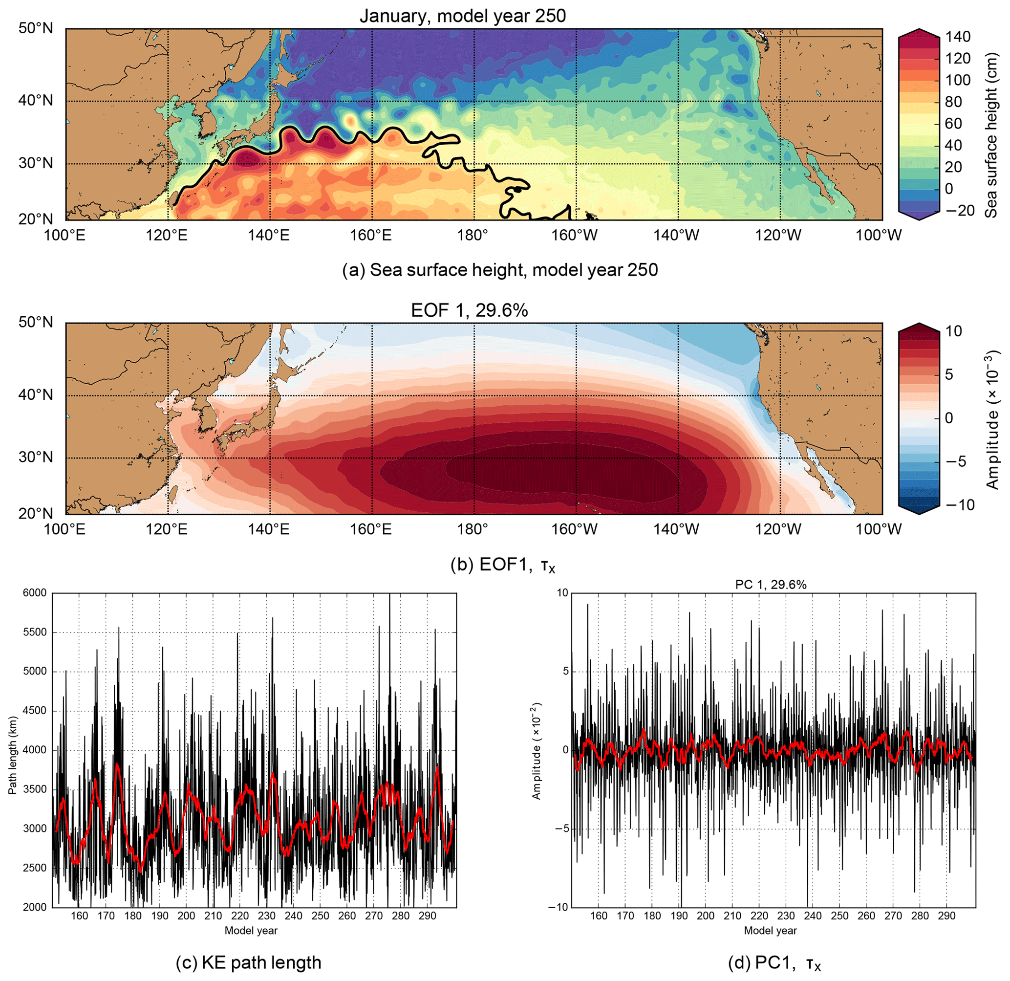
Figure 2(a) Sea surface height field in the North Pacific basin for January of model year 250. The black curve is the 70 cm SSH isoline that represents the KE jet. (b) First EOF of the zonal wind stress field over the North Pacific basin (100–260∘ E × 20–50∘ N), explaining 29.2 % of the total variance. (c) Time series of the KE path length along the region 140–160∘ E, together with its moving average of 36 months (red curve). The path length is derived from the 70 cm SSH isoline, which can be identified in (a). (d) First PC of the zonal wind stress field over the North Pacific basin (100–260∘ E × 20–50∘ N), together with its moving average of 36 months (red curve).
Before determining the Fourier spectrum, each of the time series is linearly detrended and the seasonal cycle is removed. Surrogate red noise (2000 realisations) is generated to determine the confidence levels; note that for the wind stress the lag-one autocorrelation is small, resulting in effectively white-noise surrogates. Figure 3a and b show the Fourier spectra for the two time series, and both display significant (with respect to red noise) decadal variability. Although there is a multi-decadal component of 25 years, a broad range of variability is visible in the 8–12-year window. The dominant period of the first PC of the zonal wind stress is 8 years. The spectra using the smoothed time series (using the moving average of 36 months, red curves in Fig. 2) also resulted in dominant and significant (>99 % confidence level) periods varying between 7 and 11 years for the KE path length and an 8-year period for the first PC of the zonal wind stress (not shown here).
When performing the SSA as described in Sect. 2.2 for the first PC of the zonal wind stress and the KE path length, periods of about 80–100 months (7–8 years) were found to be significant in both time series in the data basis as well as in the noise basis (Fig. 3c–f). The so-called space-time principal components (ST-PCs) corresponding to the SSA modes for a M=365 months have been used here as a representation of the 8-year period, but we have tested their robustness using various lag-window lengths M between 250 and 400 months. Values of the lag-window length M outside the considered range are not expected to give meaningful results considering the trade-off described in Sect. 2.2. For most M values, the ST-PCs that are related to this 7–8-year period are between the seventh and ninth ST-PC for the KE path length. For the zonal wind stress, the first two ST-PCs are related to this 7–8-year period. These ST-PCs pairs are used to determine the RCs, and the time series of these RCs are indicated by LM(t) for the KE path length and for the zonal wind stress, where the dependence on the lag M is made explicit. These time series will be used in the phase synchronisation analysis described in the following section.
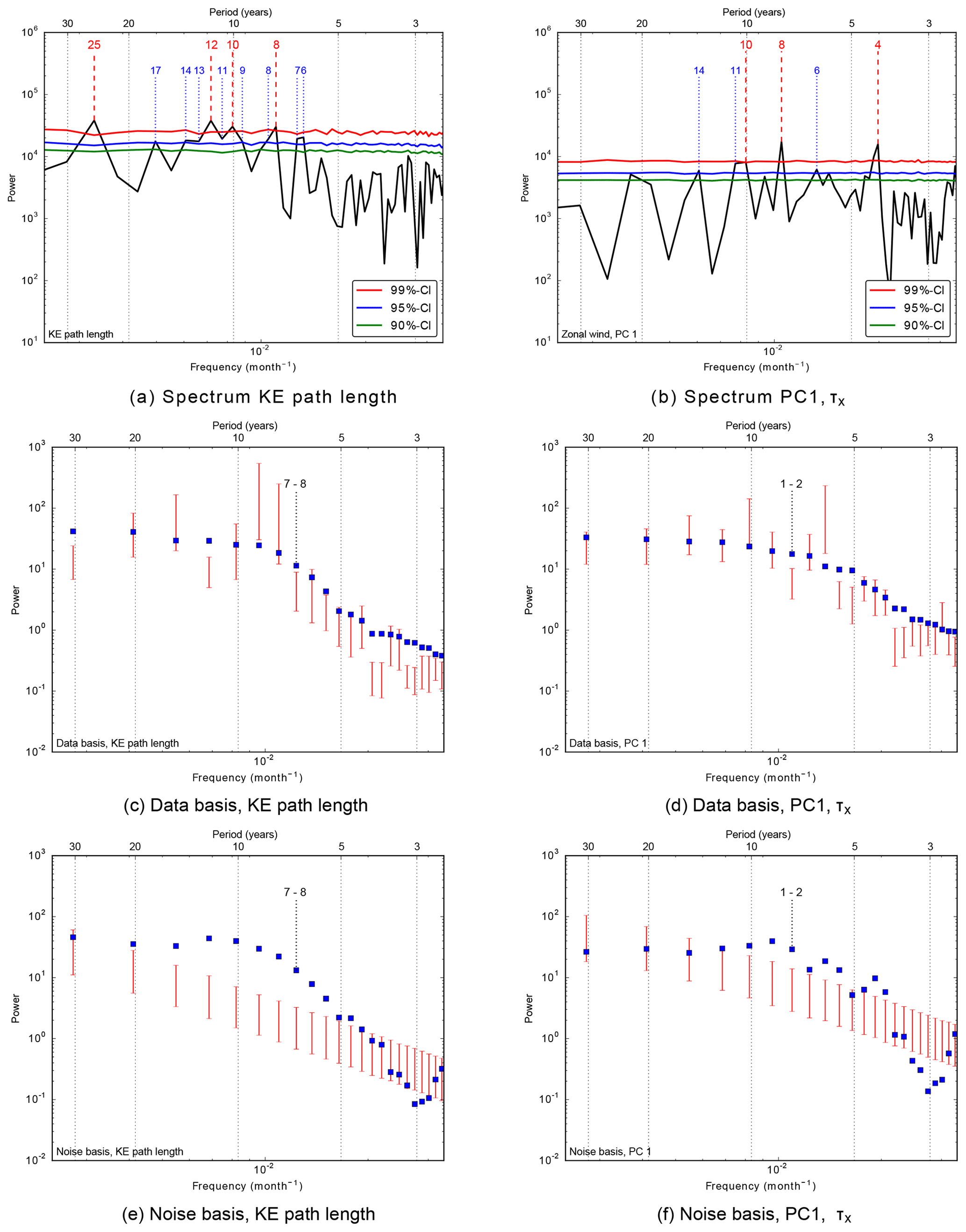
Figure 3(a, b) Fourier spectrum (black curve) of the KE path length and the first PC of the zonal wind stress (obtained from the EOF analysis). The colour-coded curves are the significance levels of red-noise surrogates, where the numbers (in years) indicate significant periods. (c, d) Data basis from the Monte Carlo SSA for the KE path length and the first PC of the zonal wind stress (obtained from the EOF analysis). (e, f) Noise basis from the Monte Carlo SSA for the KE path length and the first PC of the zonal wind stress (obtained from the EOF analysis). SSA was performed with a total lag of 365 months, and for the Monte Carlo SSA 2500 realisations have been used. The 95 % confidence intervals which have been calculated from the surrogates are shown by the red vertical bars. A specific ST-PC resulting from the SSA is represented by the blue markers and is associated with a certain frequency. The ST-PCs related to the 8-year period are significant in both the data basis and the noise basis (Allen and Robertson, 1996), and the ST-PC pair related to this variability is indicated.
3.2 Phase synchronisation
The two-dimensional embedding of the derivative of the observables with its Hilbert transform is shown in Fig. 4a and b for LM(t) (KE path length) and (zonal wind stress), respectively, for M=365 months. The trajectory in the plane spanned by the time derivative of the observable and its Hilbert transform oscillates several times around the origin so that the definition of the phase is meaningful and the instantaneous phase can be detected reliably. Note that the multi-centennial length of the model simulation and the SSA filtering is crucial to obtain a clear phase signal. Figure 4c shows the phase difference evolution between LM(t) and for three lag-window lengths (M= 275, 325 and 365 months). A (significant) plateau can be identified between model years 200 and 240 for all three values of M, indicating a phase synchronisation between the time series.
Epochs where plateaus in the phase difference occur are confirmed by the statistical test described in Sect. 2.2 using a sliding window with a length of 120 months (Fig. 4d). In this panel p values smaller than 0.0001 for each M in the KS test allow rejection of the null hypothesis related to the uniform distribution of the phase differences in the case of no synchronisation (see Sect. 2.2 for further explanations). The variation with M shows that phase synchronisation occurs for other values of M as well (Fig. 4d). Window lengths between 360 and 400 months also show a plateau from model year 190 till model year 290. Note that for some lag-window lengths (for example M=300–320 months) we did not find an appropriate ST-PC pair which is related to the 7–8-year oscillation in the SSA. The value of the phase difference, and in particular of the plateaus, is different for the three displayed lag-window lengths (M=275, 325 and 365 months) in Fig. 4c. The deviation in phase difference is caused by different ST-PCs which arise for different lag-window lengths M. However, the value of the phase difference is less important than the occurrence of a constant phase difference over a given interval (i.e. plateaus).

Figure 4(a, b) Embedding of the time derivative of the KE path length time series LM(t) (a) and that of the first PC of the zonal wind stress (b) by the Hilbert transformation. (c) Phase difference between LM(t) and for three lag-window lengths M. The black curves indicate starting points of the sliding window (length of 120 months) with p value < 0.0001. Intervals that are not significant (p value ≥ 0.0001) are indicated in red. (d) Significance of the phase difference for various lag-window lengths. Regions that are not significant (p value ≥ 0.0001) are indicated in red. The black horizontal lines indicate the values of M used in (c).
By processing the model output data by SSA as in Gelbrecht et al. (2018), certain oscillatory components are filtered out, and the phase synchronisation analysis is carried out with narrow band signals. This type of data processing introduces a risk of observing plateaus in the phase difference evolution which are interpreted as phase synchronisation but can be technically due to the similarity in the frequencies of the used signals (Paluš and Novotná, 2006). Here the Fourier spectra of the time series (cf. Fig. 3) show dominant periods of about 8 years for the KE path length and the zonal wind stress which are both significant at the 95 % confidence level. However, the spectra of the time series considered in the phase synchronisation analysis (i.e. the RCs) show differences, which limits the risk of detecting such spurious synchronisation. In addition, there is a good physical picture of the coupling between the two time series which is induced by Rossby waves (cf. Sect. 3.3). More general approaches to study the coupling between the time series can be found in Feliks et al. (2010) and Paluš and Novotná (2006).
In the analysis above, only the zonal component of the wind stress is considered, while the wind stress curl directly affects the SSH field through Ekman and Sverdrup dynamics. Therefore, we also performed a phase synchronisation analysis using the wind stress curl over the same domain as the zonal wind stress. The first EOF of the wind stress curl contains 7.6 % of the total variance, which is considerably smaller than the variance explained by the first PC of the zonal wind stress (which is 29.6 %). When conducting SSA on the first PC of the wind stress curl, a significant (95 % confidence level) ST-PC pair was identified with an 8-year period (against red-noise surrogates). A phase synchronisation analysis between the KE path length and the wind stress curl revealed significant plateaus between model years 200 and 240, similar to the results for the zonal wind stress. The similarity of the results for the zonal wind stress and the wind stress curl is expected since the meridional dependency of the zonal wind stress is the dominant component of the wind stress curl.
We also analysed phase synchronisation in the CESM between the NPGO index (Di Lorenzo et al., 2008) and the KE path length using the same procedure as above. Using the KS test, we found that there are intervals after model year 220 which significantly differ from the uniform distribution (not shown here). However, after visual inspection (which is of course a subjective measure), these epochs showed no clear plateau compared to those in Fig. 4c. Hence, compared to the PDO pattern, the NPGO pattern apparently does not contribute much to the excitation of Rossby waves as an essential part of the synchronisation mechanism (see Sect. 3.3). In addition, the dominant period of the NPGO index in the CESM output is about 19 years (95 % confidence level). Therefore it is not very likely that phase synchronisation occurs since the spectra of the KE path length shows a dominant period of about 10 years.
Finally, it should be noted that synchronisation cannot be deduced unconditionally by applying a phase synchronisation analysis and by revealing a dependence between the phases of the observables. Two time series can fulfil the “mathematical” condition of phase synchronisation which is given by the boundedness of the phase difference even if the observed state arises from other processes or effects (Rosenblum et al., 2001; Vejmelka et al., 2009). Hence, it is critical to also have a physical picture of how this synchronisation is established.
3.3 Physical mechanism of phase synchronisation
Self-sustained oscillators synchronise through a coupling which allows the adjustment of the phases. Assessing the processes responsible for the synchronisation is an important but also difficult task, especially for phase synchronisation detected from observations. A good assessment is therefore preferably carried out in an “experimental set-up” where parameters can be varied (Rosenblum et al., 2001; Vejmelka et al., 2009). Formally, the performed phase synchronisation analysis does not allow a direction of coupling between the proposed oscillators to be inferred. Causality methods such as conditional mutual information (Jajcay et al., 2018) or causal discovery algorithms (Schleussner et al., 2014; Runge et al., 2014, 2015) as well as quantifying the direction of influence (Feliks et al., 2010) between the proposed oscillators might help to reveal the direction of coupling.
However, as also mentioned above, here an adequate view of the physics of the system motivates the exploration for a possible coupling mechanism from the zonal wind stress to the KE path length through the propagation of SSH anomalies. We specifically also focus on the propagation of the anomalies of the depth of the 1028 kg m−3 isopycnal, below indicated by the IPD (isopycnal depth). First, the SSH and IPD anomalies across the basin (120–240∘ E) were averaged along latitude bands, the time mean was subtracted and the resulting anomalies were smoothed by a running mean of 36 months. The Hovmöller diagrams of the SSH and IPD anomalies averaged over the more southern latitude band of 28–30∘ N (Fig. 5) show a westward propagation of the SSH and IPD anomalies starting from the eastern part of the basin and arriving in the KCS. The travel time of these Rossby waves from the eastern to the western side of the North Pacific basin is estimated to be roughly 10 years (Chelton and Schlax, 1996), corresponding to the observed decadal variability of the Kuroshio oscillator. We also find Rossby waves for the more northward latitude bands (tested between 30 and 34∘ N), but the propagation is less clear than in Fig. 5 because of the large variability in the KCS.
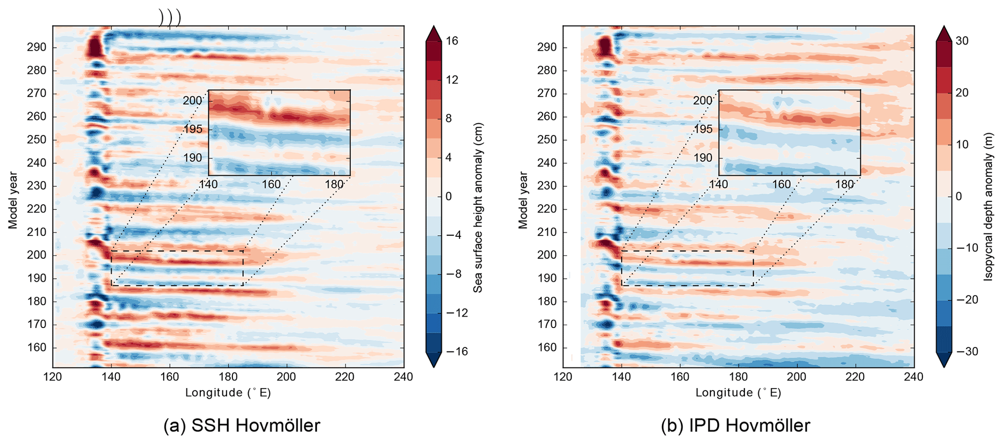
Figure 5Hovmöller diagrams of (a) SSH anomalies and (b) IPD anomalies averaged over 28–30∘ N. The result is smoothed by a running mean of 36 months. Positive (negative) anomalies in the IPD signify a deeper (shallower) isopycnal compared to the time mean. The inset emphasises the (westward) propagation of the anomalies.
The Hovmöller diagrams (Fig. 5) also indicate that positive (negative) SSH anomalies coincide with positive (negative) IPD anomalies, as expected from the baroclinic adjustment process. The stretching of the layer bounded by the surface and the 1028 kg m−3 isopycnal, which is on average roughly 500 m deep in this region, is expected to lead to variability in the horizontal velocity field through the thermal wind balance, which will affect instabilities of the KCS. To analyse how the velocity of the KCS varies due to variations in the IPD, we determined the zonally averaged zonal velocity and density between 140 and 160∘ E (i.e. Kuroshio Extension region). These zonally averaged quantities are shown in Fig. 6a and b for model years 174–176 and 181–183, respectively. These years represent a contracted state (model years 174–176) and an elongated state (model years 181–183) of the KC. For both periods of time, the upper 1000 m background flow is mainly directed eastward in the Kuroshio Extension region. Relatively warm (cold) water is found south (north) of the KC, which explains the positive meridional slope for the isopycnals. The gradient in the isopycnal slope is larger for model years 181–183 with respect to model years 174–176, in particular between 33 and 35∘ N. As a result of thermal wind balance, relative high zonal velocities are found between 33 and 35∘ N for model years 181–183 with respect to model years 174–176.
When comparing the 1028 kg m−3 IPD between model years 174–176 and 181–183, there is a clear decadal change in the background state. Variations of the 1028 kg m−3 IPD for the complete time range (model years 150–300), as shown in Fig. 6c, also display decadal variability. The maximum gradient in the 1028 kg m−3 IPD slope occurs around 34∘ N, and its value is also displayed in Fig. 6d. At the latitude where the maximum gradient of the 1028 kg m−3 IPD slope occurs (for example around 34∘ N for model years 181–183), we determined the maximum zonal velocity with depth. This maximum zonal velocity is also displayed in Fig. 6d, and both time series are significantly (95 % confidence level) correlated with a value of 0.96.

Figure 6(a, b) The zonally averaged (140–160∘ E) zonal velocity with depth, averaged over time (3-year average) for (a) model years 174–176 and (b) model years 181–183. The black curves are isopycnals each spaced by 1 kg m−3, and for reference the 1028 kg m−3 isopycnal is indicated. (c) Hovmöller diagram for the evolution of the 1028 kg m−3 isopycnal depth, smoothed by a running mean of 36 months. (d) Time series of the maximum slope of the 1028 kg m−3 isopycnal and the maximum zonal velocity at the maximum slope latitude. The time series are smoothed by a running mean of 36 months.
To determine the effects of the variations in the IPD and the background zonal velocity on the KC stability, we consider the local EKE of the KC system, defined here as
where u and v are the local monthly averaged zonal and meridional velocity, respectively, and and are their time mean. The quantities EKE and IPD are averaged over 135–145∘ E and 30–35∘ N, and the EKE is additionally averaged over the upper 500 m. For this spatially averaged IPD time series and for the KE path length time series (as in Fig. 2c), the time mean is subtracted. The three time series (EKE, IPD and KE path length) are smoothed with a running mean of 36 months and plotted in Fig. 7a. The time series for IPD and EKE are clearly out of phase, and the IPD appears to lead the EKE by about 40 months (Fig. 7b). The highest lag correlation (0.29, significant at the 95 % confidence level) between EKE and KE path length is 10 months, with EKE leading (Fig. 7b). However, taking the spatial average over a larger region (for example, 140–160∘ E × 30–35∘ N) for the EKE resulted in higher lag-correlation coefficients with the KE path length.
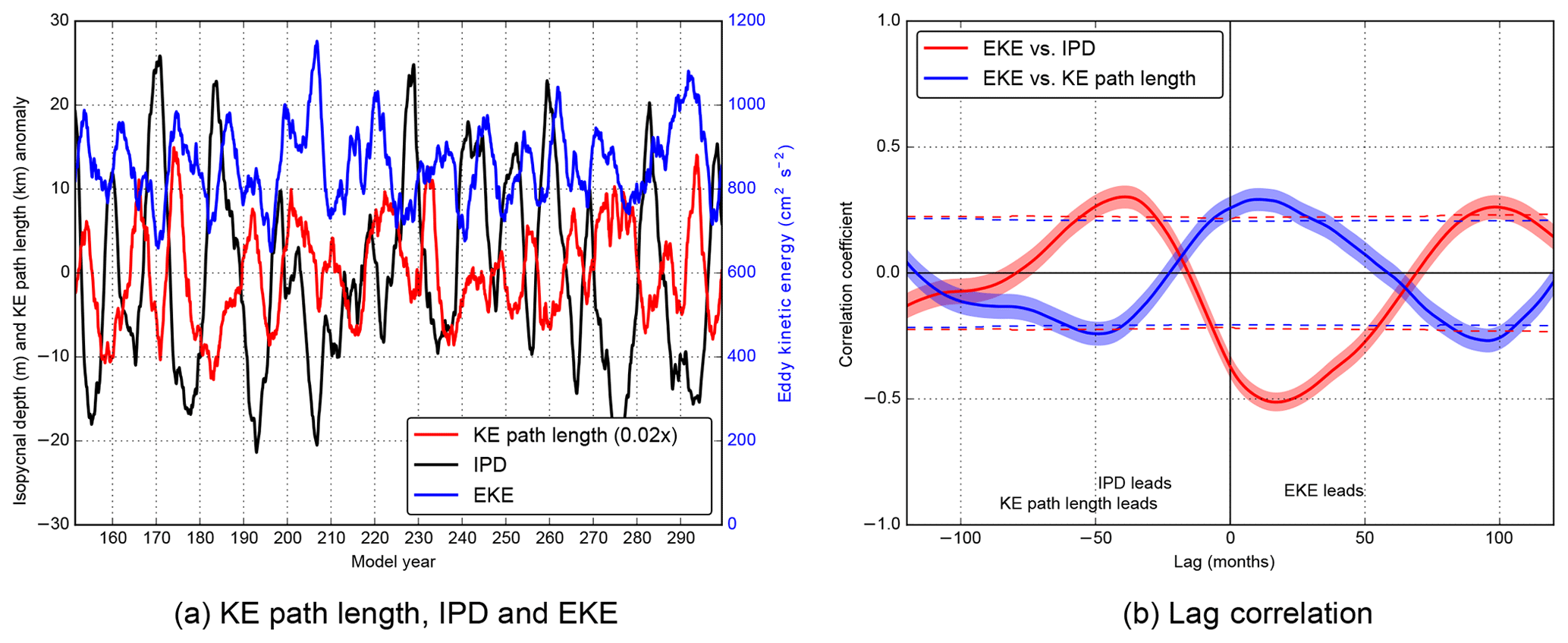
Figure 7(a) Time series of SSH, IPD and EKE. The time mean is subtracted to retain anomalies for the SSH and IPD time series. All time series are smoothed by a running mean of 36 months. (b) Lag correlation between the IPD, SSH and EKE time series. The shading indicates the 95 % confidence interval, and the dashed curves indicate significant correlations (95 % confidence level.)
We interpret the results in Figs. 6 and 7 as follows. During the deepening of the IPD (time derivative positive), the isopycnal slope also decreases, and, due to thermal wind balance, this leads to a weaker background zonal velocity with weaker horizontal and vertical shear (Fig. 6). This results in a lower intensity of mixed barotropic–baroclinic instabilities and hence relatively low values of EKE (with respect to the time mean). In more idealised configurations (Kiss and Frankcombe, 2016), one could study this in more detail by looking at the change in Floquet multipliers (associated with instabilities in the presence of periodic background forcing), but such an analysis is out of the scope of these CESM results. The non-linear interaction of growing perturbations due to the mixed barotropic–baroclinic instabilities leads to a modification of the mean state, usually referred to as rectification. In the phase of decreasing EKE, rectification effects due to the instabilities become weaker and the KC evolves into a contracted state. When the IPD shallows, precisely the opposite happens as the horizontal and vertical shear increase and the degree of instability increases, leading to a higher EKE, a stronger rectification and hence an elongated KC state. The coupling of Rossby waves to the KCS system through the motion and sloping of the isopycnals and the resulting changes in the zonal velocity field is also compatible with the analysis of other results in OGCMs (Taguchi et al., 2005, 2010), indicating that the Rossby waves can “trigger” the frontal (internal) instabilities.
Output from a multi-centennial simulation with a high-resolution version of the Community Climate System Model (CESM) was used to study phase synchronisation between path variability in the Kuroshio Current System (KCS) and the wind variability over the North Pacific basin. In particular, by performing an SSA, oscillatory components on decadal scales of the Kuroshio Extension (KE) path length and the first PC of the zonal wind stress field were chosen as representative observables for the proposed oscillators. The length of the CESM simulation is crucial for determining an adequate phase of the KE path length and the zonal wind stress variability. The high spatial resolution of the ocean model component is also needed to adequately represent the internal variability in the KCS. The phase difference evolution, the distributions of the phase difference and results from a statistical test indicate that the KE and the North Pacific zonal wind stress are episodically phase synchronised in CESM.
We interpret this phase synchronisation as an entrainment of an external frequency (that of the mid-basin wind stress variability) into the variability of a chaotic system (the KCS), as described in Sect. 5.2 of Pikovsky et al. (2001). Although there are effects of variations of the KCS on the atmospheric circulation (predominantly local) as for example described in Qiu et al. (2014), there is ample evidence that the PDO and/or NPGO variability is independent of the KCS as it is also found in low-resolution ocean/coupled models (Weijer et al., 2013). Hence, the wind stress variability acts as a forcing on the Rossby waves which couple to the KCS system through the motion of isopycnals as shown in Sect. 3.3.
When this forcing is too large with respect to the intrinsic KCS variability, the period of the external frequency is dominant and hence, in the case of a periodic forcing, the resulting KCS will become periodic in a chaos–destroying synchronisation (as described in Pikovsky et al., 2001), which it is clearly not. When the forcing is too small with respect to the intrinsic KCS variability, phase diffusion induced by non-linearities in the KCS will be dominant and prevent phase synchronisation. This likely explains why the phases are synchronised only during the main interval between model years 200 and 240. The amplitude of the zonal wind stress time series (Fig. 2d) is relatively large before the synchronisation interval (model years 200–240), and when its amplitude drops again (model years 240–250) phase synchronisation disappears. Hence, the variation in the forcing sets the epochs of the phase synchronisation. Of course, there also exist (significant) plateaus in the phase difference evolution during other time intervals. However, they are not robust across the M values, so the existence of phase synchronisation cannot be clearly demonstrated. Compared to the coupled CESM simulation, IPD anomalies have a smaller magnitude in an ocean-only (the POP model) simulation (not shown here) which was forced by a seasonal cycle (for the simulation details, see Weijer et al., 2012). In addition, they do not show a clear decadal variability; i.e. IPD anomalies in the climatological and coupled simulation are not comparable.
We think that the phase synchronisation as investigated with methods from non-linear dynamics, together with its mechanism as described in Sect. 3.3, provides a further step to connect the purely Rossby wave “forced” view of KCS path transitions, as originally advocated (Qiu and Chen, 2005, 2010), and the pure internal variability view (Pierini et al., 2009; Berloff et al., 2007). In the model world of CESM, the Rossby waves are clearly required to obtain a very pronounced decadal variability. This view is supported by (not shown) results we obtained with the OGCM only (the POP model), which was forced by a seasonal cycle. While transitions between the different KE states occur regularly in the CESM output, they develop more randomly in the POP simulation because there can be no phase synchronisation.
Indications that some periods of observed variability show a much clearer decadal variability than others are found in the analysis of AVISO data (Gentile et al., 2018). However, one cannot detect the phase synchronisation from observations yet as the AVISO time series of SSH is too short. Analysis of a 26-year interval (out of the 150-year total interval) of CESM output indicated that (with a period of variability of about 8 years) it is not possible to detect such a phase synchronisation. Unfortunately, we will have to accept that we will have to wait for a few (about 5–6) decades before this phenomenon can be demonstrated from accurate observational data.
Analysis scripts and model output are available on request from the corresponding author.
All authors generated the idea for this study and wrote the paper together.
The authors declare that they have no conflict of interest.
The authors thank Michael Kliphuis (IMAU, UU), who performed the CESM simulations, and both reviewers for their excellent suggestions and comments, which improved the manuscript substantially. The computations were done on the Cartesius at SURFsara in Amsterdam. Use of the Cartesius computing facilities was sponsored by the Netherlands Organization for Scientific Research (NWO) under the project 15502.
This paper was edited by Anna Rubio and reviewed by Stefano Pierini and one anonymous referee.
Allen, M. and Robertson, A.: Distinguishing modulated oscillations from coloured noise in multivariate datasets, Clim. Dynam., 12, 775–784, 1996. a, b
Allen, M. R. and Smith, L. A.: Monte Carlo SSA: Detecting irregular oscillations in the presence of colored noise, J. Climate, 9, 3373–3404, 1996. a
Bartsch, R., Kantelhardt, J. W., Penzel, T., and Havlin, S.: Experimental evidence for phase synchronization transitions in the human cardiorespiratory system, Phys. Rev. Lett., 98, 054102, https://doi.org/10.1103/PhysRevLett.98.054102, 2007. a
Berloff, P. S., Hogg, A. M., and Dewar, W. K.: The turbulent oscillator: a mechanism of low-frequency variability of the wind-driven ocean gyres, J. Phys. Oceanogr., 37, 2362–2386, 2007. a, b
Blasius, B., Huppert, A., and Stone, L.: Complex dynamics and phase synchronization in spatially extended ecological systems, Nature, 399, 354–359, https://doi.org/10.1038/20676, 1999. a
Boccaletti, S., Pecora, L. M., and Pelaez, A.: Unifying framework for synchronization of coupled dynamical systems, Phys. Rev. E, 63, 066219, https://doi.org/10.1103/PhysRevE.63.066219, 2001. a
Ceballos, L. I., Di Lorenzo, E., Hoyos, C. D., Schneider, N., and Taguchi, B.: North Pacific Gyre Oscillation synchronizes climate fluctuations in the eastern and western boundary systems, J. Climate, 22, 5163–5174, 2009. a
Chelton, D. B. and Schlax, M. G.: Global observations of oceanic Rossby waves, Science, 272, 234–238, 1996. a
Deser, C., Alexander, M. A., and Timlin, M. S.: Evidence for a wind-driven intensification of the Kuroshio Current Extension from the 1970s to the 1980s, J. Climate, 12, 1697–1706, 1999. a
Deser, C., Alexander, M. A., Xie, S.-P., and Phillips, A. S.: Sea Surface Temperature Variability: Patterns and Mechanisms, Annu. Rev. Mar. Sci., 2, 115–143, 2010. a
Di Lorenzo, E., Schneider, N., Cobb, K. M., Franks, P., Chhak, K., Miller, A. J., McWilliams, J. C., Bograd, S. J., Arango, H., Curchitser, E., Powell, T. M., and Rivière, P.: North Pacific Gyre Oscillation links ocean climate and ecosystem change, Geophys. Res. Lett., 35, 8, https://doi.org/10.1029/2007GL032838, 2008. Di Lorenzo, E. and Schneider, N. and Cobb, K. M. and Franks, P. J. S. and Chhak, K. and Miller, A. J. and McWilliams, J. C. and Bograd, S. J. and Arango, H. and Curchitser, E. and Powell, T. M. and Rivière, P. a, b
Feliks, Y., Ghil, M., and Robertson, A. W.: Oscillatory climate modes in the Eastern Mediterranean and their synchronization with the North Atlantic Oscillation, J. Climate, 23, 4060–4079, 2010. a, b, c, d
Gabor, D.: Theory of communication. Part 1: The analysis of information, Journal of the Institution of Electrical Engineers-Part III: Radio and Communication Engineering, 93, 429–441, 1946. a, b
Gelbrecht, M., Boers, N., and Kurths, J.: Phase coherence between precipitation in South America and Rossby waves, Sci. Adv., 4, eaau3191, https://doi.org/10.1126/sciadv.aau3191, 2018. a, b, c, d, e, f
Gentile, V., Pierini, S., de Ruggiero, P., and Pietranera, L.: Ocean modelling and altimeter data reveal the possible occurrence of intrinsic low-frequency variability of the Kuroshio Extension, Ocean Model., 131, 24–39, 2018. a, b
Ghil, M., Allen, M. R., Dettinger, M. D., Ide, K., Kondrashov, D., Mann, M. E., Robertson, A. W., Saunders, A., Tian, Y., Varadi, F., and Yiou, P.: Advanced spectral methods for climatic time series, Rev. Geophys., 40, 3.1–3.41, https://doi.org/10.1029/2000RG000092, 2002. a, b, c
Hu, D., Wu, L., Cai, W., Gupta, A. S., Ganachaud, A., Qiu, B., Gordon, A. L., Lin, X., Chen, Z., Hu, S., Wang, G., Wang, Q., Sprintall, J., Qu, T., Kashino, Y., Wang, F., and Kessler, W. S.: Pacific western boundary currents and their roles in climate, Nature, 522, 299–308, 2015. a
Jajcay, N., Kravtsov, S., Sugihara, G., Tsonis, A. A., and Paluš, M.: Synchronization and causality across time scales in El Niño Southern Oscillation, npj Climate and Atmospheric Science, 1, 33, https://doi.org/10.1038/s41612-018-0043-7, 2018. a, b, c, d
Kawabe, M.: Variations of Current Path, Velocity, and Volume Transport of the Kuroshio in Relation with the Large Meander, J. Phys. Oceanogr., 25, 3103–3117, https://doi.org/10.1175/1520-0485(1995)025<3103:VOCPVA>2.0.CO;2, 1995. a
Kiss, A. E. and Frankcombe, L. M.: The Influence of Periodic Forcing on the Time Dependence of Western Boundary Currents: Phase Locking, Chaos, and Mechanisms of Low-Frequency Variability, J. Phys. Oceanogr., 46, 1117–1136, 2016. a, b
Ma, L.: Response of ocean dynamics to multiple equilibria of the Kuroshio path South of Japan, Dyn. Atm. Oceans, 85, 1–15, 2019. a
Mantua, N. J., Hare, S. R., Zhang, Y., Wallace, J. M., and Francis, R. C.: A Pacific interdecadal climate oscillation with impacts on salmon production, B. Am. Meteorol. Soc., 78, 1069–1080, 1997. a
Maraun, D. and Kurths, J.: Epochs of phase coherence between El Nino/Southern Oscillation and Indian monsoon, Geophys. Res. Lett., 32, 15, https://doi.org/10.1029/2005GL023225, 2005. a, b
Munk, W.: On the wind-driven ocean circulation, J. Meteorol., 7, 79–93, 1950. a
Osipov, G. V., Hu, B., Zhou, C., Ivanchenko, M. V., and Kurths, J.: Three types of transitions to phase synchronization in coupled chaotic oscillators, Phys. Rev. Lett., 91, 024101, https://doi.org/10.1103/PhysRevLett.91.024101, 2003. a, b
Paluš, M.: Multiscale atmospheric dynamics: cross-frequency phase-amplitude coupling in the air temperature, Phys. Rev. Lett., 112, 078702, https://doi.org/10.1103/PhysRevLett.112.078702, 2014a. a, b
Paluš, M.: Cross-scale interactions and information transfer, Entropy, 16, 5263–5289, 2014b. a, b
Paluš, M. and Novotná, D.: Quasi-biennial oscillations extracted from the monthly NAO index and temperature records are phase-synchronized, Nonlinear Proc. Geoph., 13, 287–296, 2006. a, b, c, d, e, f, g
Paluš, M., Kurths, J., Schwarz, U., Seehafer, N., Novotná, D., and Charvátová, I.: The solar activity cycle is weakly synchronized with the solar inertial motion, Physics Letters A, 365, 421–428, 2007. a, b
Penduff, T., Juza, M., Barnier, B., Zika, J., Dewar, W. K., Treguier, A. M., Molines, J.-M., and Audiffren, N.: Sea Level Expression of Intrinsic and Forced Ocean Variabilities at Interannual Time Scales, J. Climate, 24, 5652–5670, 2011. a
Pierini, S.: A Kuroshio Extension System Model Study: Decadal Chaotic Self-Sustained Oscillations, J. Phys. Oceanogr., 36, 1605–1625, 2006. a
Pierini, S.: Kuroshio Extension bimodality and the North Pacific Oscillation: A case of intrinsic variability paced by external forcing, J. Climate, 27, 448–454, 2014. a, b, c
Pierini, S., Dijkstra, H. A., and Riccio, A.: A Nonlinear Theory of the Kuroshio Extension Bimodality, J. Phys. Oceanogr., 39, 2212–2229, 2009. a, b, c, d
Pikovsky, A., Rosenblum, M., and Kurths, J.: Synchronization, Cambridge University Press, Cambridge, 2001. a, b, c, d
Preisendorfer, R. W.: Principal Component Analysis in Meteorology and Oceanography, Elsevier, Amsterdam, the Netherlands, 1988. a
Qiu, B.: The Kuroshio Extension system: Its large-scale variability and role in the midlatitude ocean-atmosphere interaction, J. Oceanogr., 58, 57–75, 2002. a
Qiu, B. and Chen, S.: Variability of the Kuroshio Extension Jet, Recirculation Gyre, and Mesoscale Eddies on Decadal Time Scales, J. Phys. Oceanogr., 35, 2090–2103, 2005. a, b
Qiu, B. and Chen, S.: Eddy-mean flow interaction in the decadally modulating Kuroshio Extension system, Deep-Sea Res. Pt. II, 57, 1098–1110, 2010. a, b, c, d, e, f, g
Qiu, B., Chen, S., Schneider, N., and Taguchi, B.: A Coupled Decadal Prediction of the Dynamic State of the Kuroshio Extension System, J. Climate, 27, 1751–1764, 2014. a
Quiroga, R. Q., Kraskov, A., Kreuz, T., and Grassberger, P.: Performance of different synchronization measures in real data: a case study on electroencephalographic signals, Phys. Review E, 65, 041903, https://doi.org/10.1103/PhysRevE.65.041903, 2002. a
Rosenblum, M. G., Pikovsky, A. S., and Kurths, J.: Phase synchronization of chaotic oscillators, Phys. Rev. Lett., 76, 1804, https://doi.org/10.1103/PhysRevLett.76.1804, 1996. a
Rosenblum, M., Pikovsky, A., Kurths, J., Schäfer, C., and Tass, P. A.: Phase synchronization: from theory to data analysis, in: Handbook of biological physics, vol. 4, 279–321, Elsevier, Amsterdam, 2001. a, b
Runge, J., Petoukhov, V., and Kurths, J.: Quantifying the strength and delay of climatic interactions: The ambiguities of cross correlation and a novel measure based on graphical models, J. Climate, 27, 720–739, 2014. a
Runge, J., Petoukhov, V., Donges, J. F., Hlinka, J., Jajcay, N., Vejmelka, M., Hartman, D., Marwan, N., Paluš, M., and Kurths, J.: Identifying causal gateways and mediators in complex spatio-temporal systems, Nat. Commun., 6, 8502, https://doi.org/10.1038/ncomms9502, 2015. a
Schäfer, C., Rosenblum, M. G., Abel, H.-H., and Kurths, J.: Synchronization in the human cardiorespiratory system, Phys. Rev. E, 60, 857, https://doi.org/10.1103/PhysRevE.60.857, 1999. a
Schleussner, C. F., Runge, J., Lehmann, J., and Levermann, A.: The role of the North Atlantic overturning and deep ocean for multi-decadal global-mean-temperature variability, Earth Syst. Dynam., 5, 103–115, https://doi.org/10.5194/esd-5-103-2014, 2014. a
Schmeits, M. J. and Dijkstra, H. A.: Bimodality of the Kuroshio and the Gulf Stream, J. Phys. Oceanogr., 31, 2971–2985, 2001. a
Schreiber, T. and Schmitz, A.: Improved surrogate data for nonlinearity tests, Phys. Rev. Lett., 77, 635, https://doi.org/10.1103/PhysRevLett.77.635, 1996. a
Sérazin, G., Penduff, T., Barnier, B., Molines, J.-M., Arbic, B. K., Müller, M., and Terray, L.: Inverse cascades of kinetic energy as a source of intrinsic variability: A global OGCM study, J. Phys. Oceanogr., 48, 1385–1408, 2018. a, b, c, d
Simonnet, E., Dijkstra, H. A., and Ghil, M.: Homoclinic bifurcations in the quasi-geostrophic double-gyre circulation, J. Mar. Res., 63, 931–956, 2005. a
Speich, S., Dijkstra, H. A., and Ghil, M.: Successive bifurcations of a shallow-water model with applications to the wind driven circulation, Nonlin. Proc. Geophys., 2, 241–268, 1995. a
Stommel, H.: The westward intensification of wind-driven ocean currents, Trans. Amer. Geophysical Union, 29, 202–206, 1948. a
Sugimoto, S. and Hanawa, K.: Relationship between the path of the Kuroshio in the south of Japan and the path of the Kuroshio Extension in the east, J. Oceanogr., 68, 219–225, 2011. a
Sverdrup, H. U.: Wind-driven currents in a baroclinic ocean with application to the equatorial current in the eastern Pacific, P. Natl. Acad. Sci. USA, 33, 318–326, 1947. a
Taft, B. A.: Characteristics of the flow of the Kuroshio south of Japan, in: Kuroshio, physical aspects of the Japan current, edited by: Stommel, H. and Yoshida, K., Univ. Washington Press, Seattle, USA, 1972. a
Taguchi, B., Xie, S. P., Mitsudera, H., and Kubokawa, A.: Response of the Kuroshio Extension to Rossby waves associated with the 1970s climate shift in a high resolution ocean model, J Climate, 18, 2979–2995, 2005. a
Taguchi, B., Xie, S. P., Schneider, N., Nonaka, M., Sasaki, H., and Sasai, Y.: Decadal variability of the Kuroshio Extension: Observations and an eddy-resolving model hincast, J Climate, 20, 2357–2377, 2007. a, b
Taguchi, B., Nakamura, H., Nonaka, M., and Xie, S.-P.: Influences of the Kuroshio/Oyashio Extensions on Air-Sea Heat Exchanges and Storm-Track Activity as Revealed in Regional Atmospheric Model Simulations for the 2003/04 Cold Season, J. Climate, 22, 6536–6560, 2009. a
Taguchi, B., Qiu, B., Nonaka, M., Sasaki, H., Xie, S.-P., and Schneider, N.: Decadal variability of the Kuroshio Extension: mesoscale eddies and recirculations, Ocean Dynam., 60, 673–691, 2010. a
van Westen, R. M., Dijkstra, H. A., Klees, R., Riva, R. E. M., Slobbe, D. C., van der Boog, C. G., Katsman, C. A., Candy, A. S., Pietrzak, J. D., Zijlema, M., James, R. K., and Bouma, T. J.: Mechanisms of the 40–70 Day Variability in the Yucatan Channel Volume Transport, J. Geophys. Res.-Oceans, 123, 1286–1300, 2018. a, b
Vejmelka, M., Paluš, M., and Lee, W.: Phase synchronization analysis by assessment of the phase difference gradient, Chaos: An Interdisciplinary J. Nonlinear Sci., 19, 023120, https://doi.org/10.1063/1.3143903, 2009. a, b, c
Wang, S., Liu, Z., Pang, C., and Liu, H.: The decadally modulating eddy field in the upstream Kuroshio Extension and its related mechanisms, Acta Oceanol. Sin., 35, 9–17, 2016. a, b
Weijer, W., Maltrud, M. E., Hecht, M. W., Dijkstra, H. A., and Kliphuis, M. A.: Response of the Atlantic Ocean circulation to Greenland Ice Sheet melting in a strongly-eddying ocean model, Geophys. Res. Lett., 39, 9, https://doi.org/10.1029/2012GL051611, 2012. a
Weijer, W., Muñoz, E., Schneider, N., and Primeau, F.: Pacific Decadal Variability: Paced by Rossby Basin Modes?, J. Climate, 26, 1445–1456, 2013. a
Wu, L., Cai, W., Zhang, L., Nakamura, H., Timmermann, A., Joyce, T., McPhaden, M. J., Alexander, M., Qiu, B., Visbeck, M., Chang, P., and Giese, B.: Enhanced warming over the global subtropical western boundary currents, Nature Publishing Group, 2, 161–166, 2012. a
Yang, Y., San Liang, X., Qiu, B., and Chen, S.: On the Decadal Variability of the Eddy Kinetic Energy in the Kuroshio Extension, J. Phys. Oceanogr., 47, 1169–1187, 2017. a, b