the Creative Commons Attribution 4.0 License.
the Creative Commons Attribution 4.0 License.
 | 18 Sep 2020
The Ekman spiral for piecewise-uniform viscosity
David G. Dritschel
Nathan Paldor
Adrian Constantin
We re-visit Ekman's (1905) classic problem of wind-stress-induced ocean currents to help interpret observed deviations from Ekman's theory, in particular from the predicted surface current deflection of 45∘. While previous studies have shown that such deviations can be explained by a vertical eddy viscosity varying with depth, as opposed to the constant profile taken by Ekman, analytical progress has been impeded by the difficulty in solving Ekman's equation. Herein, we present a solution for piecewise-constant eddy viscosity which enables a comprehensive understanding of how the surface deflection angle depends on the vertical profile of eddy viscosity. For two layers, the dimensionless problem depends only on the depth of the upper layer and the ratio of layer viscosities. A single diagram then allows one to understand the dependence of the deflection angle on these two parameters.
- Article
(440 KB) - Full-text XML
- BibTeX
- EndNote


The motion of the near-surface ocean layer is a superposition of waves, wind-driven currents and geostrophic flows. The basic theory of wind-driven surface currents in the ocean, away from the Equator, is due to Ekman (1905) and constitutes a cornerstone of oceanography (see Vallis, 2017). Ekman dynamics is due to the balance between Coriolis and the frictional forces generated by the wind stress. Its main features, consistent with observations of steady wind-driven ocean currents, are the following:
- i.
The surface current is deflected to the right and left of the prevailing wind direction in the Northern Hemisphere and Southern Hemisphere, respectively.
- ii.
With increasing depth in the boundary layer, the current speed is reduced, and the direction rotates farther away from the wind direction following a spiral.
- iii.
The net transport is at right angles to the wind direction, to the right and left of the wind direction in the Northern Hemisphere and Southern Hemisphere, respectively.
While near the Equator wind-drift currents move in the same direction as the wind (see the discussion in Boyd, 2018), away from the Equator a deflection of steady wind-driven currents with respect to the prevailing wind direction occurs in a surface boundary layer, whose typical depth is tens of metres. Ekman's pioneering solution (see Ekman, 1905), derived for a constant vertical eddy viscosity, captures the general qualitative behaviour, but differences of detail between observations and Ekman theory were recorded in the last decades. While the characteristics (ii)–(iii) hold for any depth-dependent vertical eddy viscosity (see Constantin, 2020), there is a need to explain the occurrence of surface currents at an angle in the range 10–75∘ to the wind (rather than the 45∘ predicted by Ekman), with large variations depending on the regional and seasonal climate (see the data in Röhrs and Christensen, 2015; Yoshikawa and Masuda, 2009).
This discrepancy is typically ascribed to the effect of a vertical eddy viscosity that varies with depth. The explicit solution found by Madsen (1977), for a vertical eddy viscosity that varies linearly with depth, leads to a plausible, although somewhat low, surface current deflection angle of about 10∘. The avenue of seeking explicit solutions is not very promising, since only a few are available and the intricacy of the details makes it difficult to extract broad conclusions (we refer to Constantin and Johnson, 2019; Grisogno, 1995, for a survey of known Ekman-type solutions). The challenging nature of the task is highlighted by the recent analysis pursued in Bressan and Constantin (2019) and Constantin (2020) where asymptotic approaches, applicable for eddy viscosities that are small perturbations of a constant, revealed the convoluted way in which the eddy viscosity influences the deflection angle: while a slow and gradual variation of the eddy viscosity with depth results in a deflection angle larger than 45∘, the typical outcome of an eddy viscosity concentrated in the middle of the boundary layer is a deflection angle below 45∘. A better understanding of the deflection angle is important theoretically but also for operational oceanography, e.g. in the context of search-and-rescue operations or in remedial action for oil spills.
The important issue of a quantitative relation between the vertical eddy viscosity and the magnitude of the deflection angle remains open. The aim of this paper is to discuss this issue in cases when the eddy viscosity is piecewise uniform. The in-depth analysis that can be pursued in this relatively simple setting permits us to gain insight into the way the turbulent parametrization (e.g. of general circulation models) controls the deflection angle. This paper is organized as follows: in Sect. 2 we present the Ekman equations for wind-driven oceans having depth-dependent eddy viscosities, and we perform a suitable scaling that reduces the number of parameters. In Sect. 3, an explicit solution is constructed and illustrated for an infinitely deep ocean with two constant values of eddy viscosity. This solution covers the full range of possibilities and exhibits deflection angles covering the full range between 0 and 90∘. Various special or limiting cases are highlighted. Finally, Sect. 4 offers our conclusions.
For a deep, vertically homogeneous ocean, of infinite lateral extent, the horizontal momentum equation for steady flow takes the following (complex) form under the f-plane approximation:
where is the complex horizontal velocity in the (X,Y) plane, Z is the depth below the mean surface Z=0, f is the Coriolis parameter, ρ is the (constant) density, is the horizontal pressure gradient, is the shear stress due to molecular and turbulent processes, and the higher-order terms, representing interactions between the variables, are presumed to be small. Decomposing the horizontal velocity into pressure-driven (geostrophic) and wind-driven (Ekman) components , we see from Eq. (1) that the leading-order geostrophic and wind-driven flows separate, with the linear equation
governing the dynamics of the wind-driven flow. By relating the stress vector within the fluid, τ, to the shear profile through a turbulent eddy viscosity coefficient ν(Z),
from Eq. (2) we obtain Ekman's equations for wind-driven ocean currents
Let us now discuss the appropriate boundary conditions. At the surface, the shear stress balances the wind stress, τ0:
The “bottom” boundary condition expresses the vanishing of the wind-driven current with depth (necessary to keep the total kinetic energy finite), where the flow is essentially geostrophic:
Letting τ0 denote the magnitude of the surface wind stress, we non-dimensionalize the problem by scaling Ue by and Z by , since τ0∕ρ has units of L2∕T2. The factor of 2 is introduced for convenience below. Upon defining a dimensionless eddy viscosity , velocity and depth , the equations transform to
where ψ=uK(0) and a prime means a derivative with respect to z (cf. Eqs. 14–16 in Gill, 1982). The scaling performed does not change the surface deflection angle θ0, equal to the argument of the complex vector ψ(0), even if the scaling results in an orientation of the horizontal axes such that the surface wind stress points in the positive x direction. Finally, we note that this formulation is appropriate for the Northern Hemisphere where f>0. The formulation for the Southern Hemisphere is obtained by taking the complex conjugate in Eq. (7), noticing that K is real-valued.
For piecewise-constant K, without loss of generality we can further scale z so that K=1 in while K=ℓ2 in , where h is the dimensionless depth of the upper layer. Note that ℓ is the ratio of the lower-layer to upper-layer viscous lengths. The analysis below can be readily extended to any number of regions of constant K, but the simplest to understand is two regions, since then the solution depends on only two dimensionless parameters, ℓ and h.
3.1 Constructing the solution
In each region, the complex velocity ψ satisfies a simple constant-coefficient equation:
having exponential solutions
where A, B and C are (generally complex) constants. The boundary condition ψ→0 as has been used to eliminate the growing solution in Eq. (13).
At the discontinuity in K, at , we require continuity of ψ, i.e. . Moreover, by integrating the equation above across an infinitesimal region centred on , we obtain
The upper surface boundary condition implies
while continuity of ψ at implies
and finally the jump condition (Eq. 14) on ψ′ at implies
It follows that
Applying the surface boundary condition (Eq. 15) determines C as
The surface current deflection angle, θ0, measured clockwise, is determined from
But given C above in Eq. (19), we have
Introducing the real values and enables us to write
which, after multiplying top and bottom by the complex conjugate of the denominator, simplifies to
Hence, taking the (negative of the) ratio of the imaginary to real parts of this, we obtain
3.2 Results
First, we examine certain special cases.
When ℓ=1, there is no discontinuity in eddy viscosity. Since in this case β=0, we have tan θ0=1, i.e. in agreement with the classical Ekman spiral solution.
As ℓ→0, the eddy viscosity vanishes in the lower layer, and the flow field ψ must also vanish. In this case, tan θ0 reduces to
which has a non-trivial dependence on h. The maximum value is attained as h→0; then tan θ0→∞ or θ0→90∘.
As ℓ→∞, corresponding to an extremely viscous lower layer, tan θ0 reduces to the inverse of the previous expression, i.e.
The minimum occurs for h→0 and there tan θ0→0 or θ0→0.
For general ℓ, there are also values of h for which tan θ0=1. These occur when the numerator and the denominator of the general expression above for tan θ0 are equal. But this means αβsin (2h)=0 or . One solution is the classical Ekman spiral with ℓ=1 noted above. But we also have for non-negative integers n. When n=0, the upper layer vanishes and the eddy viscosity is uniform throughout the entire depth. The classical Ekman spiral is expected in this case. The other special depths imply θ0 exhibits a non-monotonic dependence on h for fixed ℓ. In fact, tan θ0 exhibits a decaying oscillation about a value of unity.
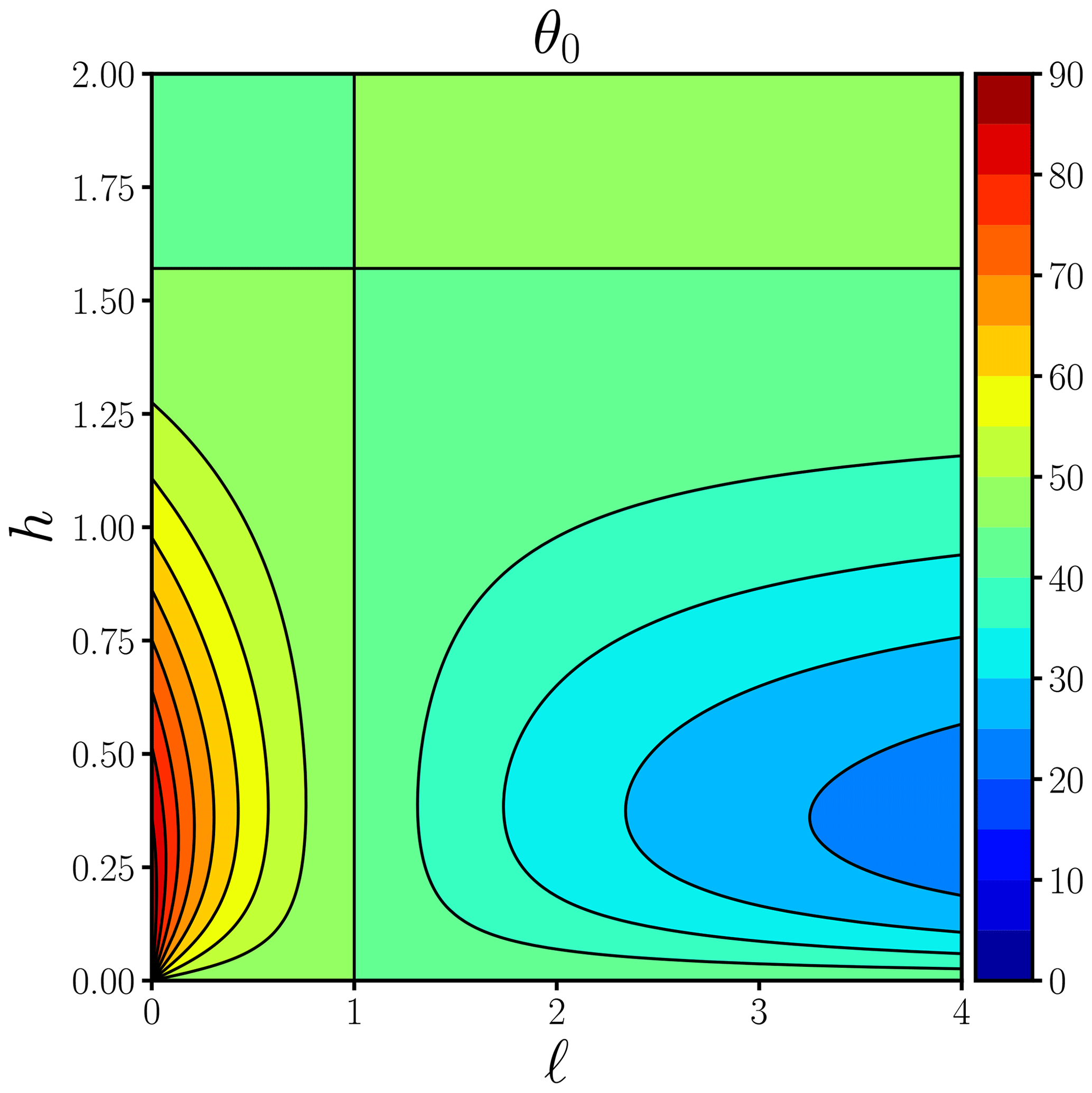
Figure 1Surface deflection angle θ0 (in degrees) as a function of the lower-layer non-dimensional viscous length ℓ and the non-dimensional depth of the upper layer h.
A summary of the results in the ℓ–h plane is provided in Fig. 1. Along any line ℓ = constant (excluding ℓ=1), θ0 reaches a minimum or maximum in h when the following relation holds:
obtained by setting the partial derivative of tan θ0 with respect to h equal to zero. The first extremum with increasing h occurs for (when the above equation yields ℓ=1). Note that as h→0, , implying either ℓ→0 or ℓ→∞ as noted previously. Extrema also occur for larger h since the function in the square root above is periodic, but these involve much weaker variations in θ0 about 45∘, diminishing like e−nπ for positive integers n. When n=1, the maximum excursion in tan θ0 is approximately 0.05735.
We have re-visited the famous problem originally posed by Nansen (see the discussion in Huntford, 2002) and solved by Ekman (1905) to understand wind-driven currents in the ocean. By balancing viscous and Coriolis forces, and assuming a constant vertical eddy viscosity, Ekman (1905) predicted that the surface current is deflected by 45∘ to the right and left of the prevailing wind direction in the Northern Hemisphere and Southern Hemisphere, respectively. Moreover, Ekman (1905) found that the net fluid transport is 90∘ to the right and left of the wind direction.
Since then, a number of studies have sought to explain observed discrepancies with Ekman's theory (Röhrs and Christensen, 2015; Yoshikawa and Masuda, 2009), in particular deflection angles significantly different from the 45∘ prediction (Madsen, 1977; Grisogno, 1995; Bressan and Constantin, 2019; Constantin and Johnson, 2019; Constantin, 2020). The main conclusion is that these discrepancies can be explained by vertically varying eddy viscosities. However, due to the mathematical difficulty in constructing exact or asymptotic solutions, no general scenario has yet emerged relating the deflection angle to the profile of eddy viscosity.
This study makes a first step in this direction by considering the case of piecewise-constant eddy viscosities for which analytical solutions may be readily constructed and analysed. We have presented results for the simplest situation of two regions having different uniform viscosities in an infinitely deep ocean. (In fact the results also apply when the two regions have different densities, such as a mixed layer of density ρ1 overlying a denser deep layer of density ρ2. In that case the lower-layer dimensionless viscosity ℓ2 includes the density ratio ρ1∕ρ2.) By an appropriate scaling of the governing equations, the solutions can be shown to depend on only two parameters: the ratio of the lower-to-upper viscous lengths ℓ and the dimensionless depth of the upper layer h. This permits one to see at a glance how both ℓ and h determine the surface deflection angle θ0.
In appropriate limits, we recover Ekman's classical solution, but additionally the 45∘ deflection angle may also occur for arbitrary ℓ, when h assumes special values. In general, for h sufficiently small and ℓ<1 (a less viscous lower layer), the deflection angle exceeds 45∘ (and can reach nearly 90∘ for ℓ≪1). When ℓ>1 (a more viscous lower layer), the deflection angle is less than 45∘ and tends to zero as ℓ→∞ for h≪1. For ℓ∼1 our conclusions are in agreement with the results obtained recently in Bressan and Constantin (2019) and Constantin (2020). Indeed, writing for z≤0, with and
the perturbative approach developed in Bressan and Constantin (2019) and Constantin (2020) shows that a positive and negative value of the integral
corresponds to a deflection angle larger and smaller than 45∘. respectively. The relation
shows that this is consistent with our conclusions.
The results obtained may help better formulate appropriate parameterizations of eddy viscosities in global circulation models of the ocean. For example, it is typical for the upper 100 m of the ocean that solar heating quenches turbulence during the day (see the discussion in Woods, 2002). Our model captures these changes: during the day we set ℓ>1, with ℓ<1 during the night, thus explaining the observation that often the deflection angle exceeds 45∘ during the day, and is below 45∘ during the night (see Krauss, 1993). The same reasoning applies to the large seasonal variations of the deflection angle observed at some locations (see the data in Yoshikawa and Masuda, 2009) and explains why one observes angles below 45∘ in arctic regions, where the ice cover quells the turbulence near the ocean surface. On the other hand, the regularity of strong winds in the Drake Passage makes the assumption of a uniform eddy viscosity reasonable (i.e. ℓ=1) so that in this region the deflection angle is typically close to 45∘ (see the data in Polton et al., 2013; Roach et al., 2015). We are not aware of detailed observational studies relating the deflection angle to the vertical profile of eddy viscosity, but we hope that our work will serve as a guide.
All authors contributed equally to this work.
The authors declare that they have no conflict of interest.
The authors would like to thank the three anonymous referees for their helpful comments on our paper.
This research has been supported by the UK Engineering and Physical Sciences Research Council (grant no. EP/H001794/1).
This paper was edited by Neil Wells and reviewed by three anonymous referees.
Boyd, J. P.: Dynamics of the Equatorial Ocean, Springer, Berlin, 2018. a
Bressan, A. and Constantin, A.: The deflection angle of surface ocean currents from the wind direction, J. Geophys. Res.-Oceans, 124, 7412–7420, 2019. a, b, c, d
Constantin, A.: Frictional effects in wind-driven ocean currents, Geophys. Astro. Fluid, https://doi.org/10.1080/03091929.2020.1748614, online first, 2020. a, b, c, d, e
Constantin, A. and Johnson, R. S.: Atmospheric Ekman flows with variable eddy viscosity, Bound.-Lay. Meteorol., 170, 395–414, 2019. a, b
Ekman, V. W.: On the influence of the Earth's rotation on ocean-currents, Ark. Mat. Astron. Fys., 2, 1–52, 1905. a, b, c, d, e, f
Gill, A. E.: Atmosphere-Ocean Dynamics, Academic Press, New York, USA, 1982. a
Grisogno, B.: A generalized Ekman layer profile with gradually varying eddy diffusivities, Q. J. Roy. Meteor. Soc., 121, 445–453, 1995. a, b
Huntford, R.: Nansen: The Exporer as Hero, Abacus, London, UK, 2002. a
Krauss, W.: Ekman drift in homogeneous water, J. Geophys. Res., 98, 187–209, 1993. a
Madsen, O. S.: A realistic model of the wind-induced Ekman boundary layer, J. Phys. Oceanogr., 7, 248–255, 1977. a, b
Polton, J. A., Lenn, Y.-D., Elipot, S., Chereskin, T. K., and Sprintall, J.: Can Drake Passage observations match Ekman's classic theory?, J. Phys. Oceanogr., 43, 1733–1740, 2013. a
Roach, C. J., Phillips, H. E., Bindoff, N. L., and Rintoul, S. R.: Detecting and characterizing Ekman currents in the Southern Ocean, J. Phys. Oceanogr., 45, 1205–1223, 2015. a
Röhrs, J. and Christensen, K. H.: Drift in the uppermost part of the ocean, Geophys. Res. Lett., 42, 10349–10356, 2015. a, b
Vallis, G. K.: Atmospheric and Oceanic Fluid Dynamics, Cambridge University Press, Cambridge, UK, 2017. a
Woods, J.: Laminar flow in the ocean Ekman layer, in: Meteorology at the Millenium, edited by: Pearce, R. P., Academic Press, San Diego, USA, 220–232, 2002. a
Yoshikawa, Y. and Masuda, A.: Seasonal variations in the speed factor and deflection angle of the wind-driven surface flow in the Tsushima Strait, J. Geophys. Res., 114, C12022, https://doi.org/10.1029/2009JC005632, 2009. a, b, c