the Creative Commons Attribution 4.0 License.
the Creative Commons Attribution 4.0 License.
 | 21 Feb 2019
Long Island Sound temperature variability and its associations with the ridge–trough dipole and tropical modes of sea surface temperature variability
Justin A. Schulte
Sukyoung Lee
Possible mechanisms behind the longevity of intense Long Island Sound (LIS) water temperature events are examined using an event-based approach. By decomposing an LIS surface water temperature time series into negative and positive events, it is revealed that the most intense LIS water temperature event in the 1979–2013 period occurred around 2012, coinciding with the 2012 ocean heat wave across the Mid-Atlantic Bight. The LIS events are related to a ridge–trough dipole pattern whose strength and evolution can be determined using a dipole index. The dipole index was shown to be strongly correlated with LIS water temperature anomalies, explaining close to 64 % of cool-season LIS water temperature variability. Consistently, a major dipole pattern event coincided with the intense 2012 LIS warm event. A composite analysis revealed that long-lived intense LIS water temperature events are associated with tropical sea surface temperature (SST) patterns. The onset and mature phases of LIS cold events were shown to coincide with central Pacific El Niño events, whereas the termination of LIS cold events was shown to possibly coincide with canonical El Niño events or El Niño events that are a mixture of eastern and central Pacific El Niño flavors. The mature phase of LIS warm events was shown to be associated with negative SST anomalies across the central equatorial Pacific, though the results were not found to be robust. The dipole pattern was also shown to be related to tropical SST patterns, and fluctuations in central Pacific SST anomalies were shown to evolve coherently with the dipole pattern and the strongly related East Pacific–North Pacific pattern on decadal timescales. The results from this study have important implications for seasonal and decadal prediction of the LIS thermal system.
- Article
(12502 KB) - Full-text XML
- BibTeX
- EndNote


Fluctuations in sea surface temperature (SST) across coastal portions of the United States (US) are driven by changes in oceanic and atmospheric circulation patterns. Changes in water temperature along the US west coast are related to the Pacific Decadal Oscillation (PDO) and the North Pacific Gyre Oscillation, as is well documented (Mantua et al., 1997; Mantua and Hare, 2002; Di Lorenzo, 2008). For the US east coast, water temperature fluctuations are related to changes in the Gulf Stream position and variations in the Atlantic Multidecadal Oscillation, PDO, and East Pacific–North Pacific (EP–NP) pattern (Pershing et al., 2015; Schulte et al., 2018). Superimposed on the water temperature changes driven by natural modes of variability is background warming associated with anthropogenic climate change (Pershing et al., 2015).
Although the mechanisms behind SST variability along the US west coast are well documented, comparatively fewer studies have focused on understanding SST variability across the Mid-Atlantic Bight in the context of large-scale climate modes. Two recent studies put water temperature variability across the Gulf of Maine and the Long Island Sound (LIS) in a climate-mode context. The first study by Pershing et al. (2015) showed that the combination of Gulf Stream and PDO influences led to the rapid warming of the Gulf of Maine that resulted in the collapse of the cod fishery.
More recently, a second study by Schulte et al. (2018) found the EP–NP pattern to be a dominant pattern governing LIS water temperature variability. The EP–NP pattern was shown to be strongly correlated with LIS water temperature unlike the well-known North Atlantic Oscillation (NAO; Hurrell, 1995), Pacific North American (PNA; Wallace and Gutzler, 1981; Svoma, 2011), Arctic Oscillation (AO; Thompson and Wallace, 1998), and West Pacific (WP; Barston and Livezey, 1987; Linkin and Nigam, 2008) patterns. In fact, Schulte and Lee (2017) found that the EP–NP pattern is more strongly related to temperature variability across the northeast US than the AO, which is often associated with colder-than-normal conditions across the region (Wettstein and Mearns, 2002). Those results suggest that the EP–NP pattern is an important component to seasonal prediction of air and water temperature across the LIS region. Another important aspect of the EP–NP pattern is its strong decadal variability, which could enable decadal prediction of LIS water temperature. Schulte et al. (2018) termed the decadal component of the EP–NP pattern the quasi-decadal mode and showed that it fluctuates coherently with LIS water temperature anomalies. The physical mechanism contributing to the EP–NP decadal variability was not identified, underscoring the need for an additional study to identify a possible source of the EP–NP decadal variability. Understanding the mechanisms behind the EP–NP decadal variability has implications for seasonal and decadal prediction of LIS water temperature.
Improving the current understanding of the climatic mechanisms governing LIS water temperature variability also has important implications for managing fisheries. For example, Howell and Auster (2012), using finfish abundance indices, found shifts in spring community structures that are related to water temperature. The LIS American lobster, which is sensitive to water temperature, dramatically declined around 1997 (Pearce and Balcom, 2005), but managing the lobster harvests has failed to recover the lobster fishery. For the nearby Rhode Island Sound, biological communities are related to spring–summer water temperature (Collie et al., 2008), suggesting that predicting spring–summer water temperature could aid the setting of fish harvest quotas. These studies underscore the need to better understand water temperature variability across the LIS region so that changes in biological communities can be better monitored and used to better manage fish harvests.
Another reason that the LIS is important to study is that it is in a region where air temperature and precipitation are not strongly influenced by well-known climate modes such as the NAO, AO, PNA, and WP that are extracted from the widely used classical empirical orthogonal function (EOF) analysis method (Barston and Livezey, 1987). Schulte et al. (2016) found weak relationships between well-known climate indices and the variability of precipitation and temperature across the northeast US. As shown by Schulte et al. (2018), LIS water temperature variability is strongly related to neither changes in the Gulf Stream position nor fluctuations in the NAO despite being located adjacent to the Atlantic Ocean. The weak Gulf Stream influence is likely the result of the LIS being a semi-enclosed water basin, whereas the general movement of weather systems from west to east may reflect the weak NAO influences because the NAO's centers of action are located downstream of the LIS.
Recognizing that well-known climate indices are weakly related to the salinity variability of northeast US estuaries, Schulte et al. (2017a) adopted a continuum approach (Franzke and Feldstein, 2005; Johnson and Feldstein, 2010; Johnson et al., 2008) to teleconnection pattern extraction and identified an eastern North American (ENA) sea level dipole pattern that is more strongly correlated with streamflow than the PNA and NAO indices. In a subsequent study, Schulte et al. (2017b) found the ENA pattern to be strongly related to northeast US precipitation and LIS salinity. Those results suggest that a continuum approach is better suited for understanding climate variability and associated LIS water temperature impacts than an EOF-based analysis. Although Schulte et al. (2018) did show that the EOF-based EP–NP pattern is strongly correlated with LIS water temperature, the EP–NP pattern for December cannot be unambiguously extracted using the rotated principal component analysis (RPCA) conducted by the Climate Prediction Center (CPC). Furthermore, EOF analysis assumes atmospheric patterns are orthogonal even though orthogonality does not hold for the real atmosphere. This orthogonality assumption can lead to the generation of unphysical modes (Tremblay, 2001). In contrast, clustering methods such as self-organizing maps (SOMs) that view the atmosphere as a continuum more accurately produce patterns that are actually observed than EOF analysis (Liu et al., 2006; Johnson et al., 2008; Yuan et al., 2015).Therefore, an additional study is needed to construct an atmospheric circulation index that is strongly related to LIS water temperature variability, physically based, and unambiguously defined for all months.
In this paper, we use an event-based approach to identify LIS water temperature relationships with atmospheric and oceanic patterns. More specifically, the main objectives of the study are the following: (1) identify the atmospheric circulation patterns associated with LIS water temperature events; (2) create a simple atmospheric index that is strongly correlated with LIS water temperature; and (3) use the simple atmospheric index to better understand LIS water temperature variability. Because tropical Pacific SST patterns are often used in seasonal forecasting over North America, we address the question as to whether there is an SST pattern precursor to LIS temperature events.
In this paper, SST fields from 1870 to 2013 are based on the Hadley Centre Global Sea Ice and Sea Surface Temperature (HadISST1) data set (Rayner et al., 2016). Atmospheric fields were analyzed using 500 hPa geopotential height and sea level pressure (SLP) fields based on the National Oceanic Atmospheric Administration's 20th century reanalysis (Compo et al., 2011) and the National Center for Atmospheric Prediction (NCEP; Kalnay et al., 1996) reanalysis. The 20th century reanalysis product was used because the product extends back to 1851, whereas the NCEP reanalysis product only extends back to 1948. Mean monthly air temperature data from 1979 to 2013 were based on the observed US climate divisional data set (Guttman and Quayle, 1996). The data set comprises average monthly temperature data for 344 climate regions (Fig. 1a) that partition the US into homogeneous climate zones. The annual cycles were removed from the data by subtracting the mean monthly values for each month from the monthly values of the corresponding month for each grid point or climate division.
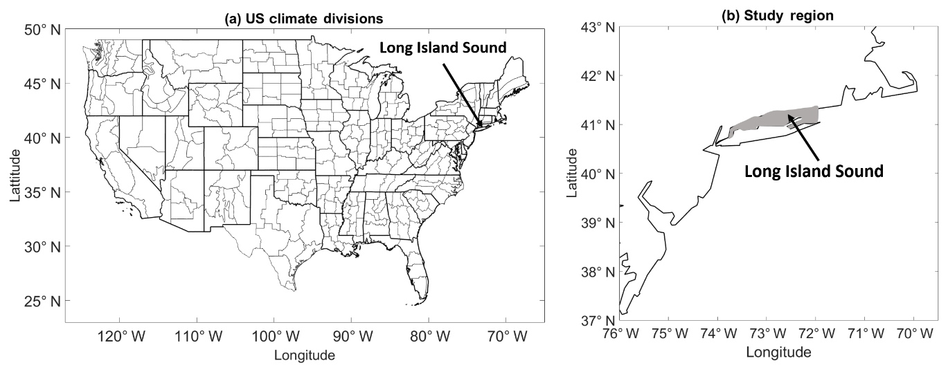
Figure 1(a) The 344 US climate divisions and (b) the LIS study region. Gray shading delineates the region used to calculate the LIS surface water temperature time series.
LIS surface water temperature data used in this study were generated from the New York Harbor Observing Prediction System (NYOPS; Georgas et al., 2016). Model-generated data were preferred to observational data because observations are temporally sparse and continuous data are needed for the methods adopted in this study. The NYHOPS model is a three-dimensional hydrodynamic model with 11 vertical levels. Following Schulte et al. (2018), water temperature computed on the first vertical level was considered surface water temperature. The LIS is a well-mixed estuary, so the choice of vertical level is not critical to the results presented in this study. To obtain a single time series representing LIS surface water temperature (for brevity, referred to as LIS temperature hereafter), water temperature was averaged over the gray-shaded region shown in Fig. 1b. The annual cycle in the resulting LIS temperature time series was removed using 1979–2013 monthly means.
The LIS temperature time series and the SST fields were detrended to remove the long-term trend. The time series were detrended by fitting a least-squares fit of a line to the time series and subtracting the line from the time series. To check the sensitivity of results to detrending, the analyses were conducted using both the detrended and non-detrended data. Results for the detrended analysis are shown unless otherwise specified. The reason for showing the detrended results is that the study is focused on interannual variability rather than long-term trends.
Indices for the NAO, AO, EP–NP, PNA, and the WP were obtained from the CPC and were based on the 1979–2013 period. The NAO, WP, PNA, and EP–NP indices obtained from the CPC were calculated from an RPCA of 500 hPa geopotential height anomalies poleward of 20∘ N. The AO index was calculated from an RPCA of 1000 hPa geopotential height anomalies. Data for the 1950–2013 period were also used for the EP–NP index.
The Niño 3 and Niño 4 indices from 1870 to 2013 (available at https://www.esrl.noaa.gov/psd/gcos_wgsp/Timeseries/, last access: 15 November 2018) were used to measure the strength and evolution of the El-Niño–Southern Oscillation (ENSO). Whereas the Niño 3 index better describes the evolution of canonical ENSO, the Niño 4 index better describes the evolution of central Pacific ENSO events (Kao and Yu, 2009; Lee and McPhaden, 2010) Thus, using these two indices, we accounted for two different flavors of ENSO. The annual cycles from these ENSO metrics were removed using the long-term (1870–2013) monthly means.
3.1 Event decomposition
To better understand the characteristics of climate time series, time series were decomposed into negative and positive events. More specifically, let a time series X be a sequence of N data points x1, x2, …,xN at the time points t1, t2, …, tN, with the data points assumed to be equally spaced. Data points were based on monthly anomalies so that they were both positively and negatively valued. Thus, a complete sequence x1, x2, …, xN was partitioned into subsequences comprising adjacent data points whose values are of similar sign. Such subsequences were termed positive or negative events depending on the values of the data points.
The onset and decay of events were defined as follows. A negative event Eneg was said to begin at tj if xj<0 and . A negative event beginning at tj was said to terminate at tk≥tj if xk<0, , and xi<0 for all i such that . A similar definition was used to define positive events, but the sign conventions were reversed. The time point tj was termed the onset phase and the time point tk was termed the decay phase. The peak intensity of a negative (positive) event was deemed the minimum (maximum) value obtained by a data point within the event period [tj tk]. If the peak intensity of an event occurred at tp, then tp was termed the mature phase.
Given this definition of an event, an event occurring over the time period [tj tk] contained data points, with the integer M regarded as the persistence of the event. The cumulative intensity (referred to as the intensity hereafter) of an event E was defined as
where yi is a data point composing the event E. The absolute value of intensity was deemed the magnitude of an event. The duration and intensity of events were depicted using an event spectrum. The event spectrum was comprised of line segments beginning at the onset phases and ending at the termination phases of the events. That is, for each event, a line segment was drawn from the point (tj,I) to the point (tk,I) so that the length of the line segment represented the event duration.
There are several advantages to using the event decomposition approach. The first advantage is that the autocorrelation of the data is accounted for by grouping the data into events. The second advantage is that the persistence of individual events can be readily defined, whereas the lag-1 autocorrelation coefficient measure of persistence needs to be calculated using a data interval so that the lag-1 autocorrelation coefficient may not reflect the persistence of an individual event. A third advantage is that potential nonlinearities are accounted for by analyzing negative and positive events separately.
3.2 Wavelet analysis
To extract time-frequency information from a time series X, a wavelet analysis (Torrence and Compo, 1998) was implemented. The wavelet transform of X is given by
where ψ is the Morlet wavelet given by
where ω0=6 is the dimensionless frequency, t is time, s is wavelet scale, δt is a time step (1 month in this study), , and the asterisk denotes the complex conjugate (Torrence and Compo, 1998).
To quantify the relationships between climate modes and water temperature as a function of frequency and time, a wavelet coherence analysis was conducted. Following Grinsted et al. (2004), the (local) wavelet squared coherence between two time series X and Y is given by
where is the cross-wavelet transform defined as the product of the wavelet transform of X and the complex conjugate of the wavelet transform of Y. In Eq. (4), S is a smoothing operator that smooths coherence in time and in wavelet scale (Grinsted et al., 2004). Using Monte Carlo methods, the statistical significance of wavelet squared coherence was assessed by generating 10 000 pairs of surrogate red-noise time series with the same lag-1 autocorrelation coefficients as the input time series and computing the wavelet squared coherence between each pair (Grinsted et al., 2004).
To reduce the number of false positive results arising from the simultaneous testing of multiple hypotheses (Maraun and Kurths, 2004; Maraun et al., 2007; Schulte et al., 2015; Schulte, 2016), the cumulative area-wise test developed by Schulte (2016) was applied. The test tracked how the areas of contiguous regions of point-wise significance (significance patches) changed as the point-wise significance level was altered. The test was applied by computing the normalized areas of point-wise significance patches over a discrete set of point-wise significance levels. The normalized area of a patch was defined as the patch area divided by the square of its centroid's scale coordinate (Schulte et al., 2015; Schulte, 2016). In this study, the normalized areas were computed using point-wise significance levels ranging from α=0.02 to α=0.18. The spacing between adjacent point-wise significance levels was set to 0.02.
The strength of coherence was also measured using global coherence (Schulte et al., 2016), the time-averaged representation of local wavelet squared coherence. Global coherence is given by
where
(Schulte et al., 2016). The statistical point-wise significance of GC(s) was computed using Monte Carlo methods in a similar manner to local wavelet squared coherence.
A lower-dimensional version of the cumulative area-wise test was applied to the global coherence spectra to reduce the number of false positive results (Schulte et al., 2018). The test assessed the statistical significance of one-dimensional arcs using arc length, which is an integrated metric accounting for the width of the peak in wavelet scale (frequency) and the extent to which the peak is above the critical level of the point-wise test. To track how the arc length of a given point-wise significance peak changed as the point-wise significance level was altered, the arc length of the point-wise significance peak was computed at point-wise significance levels ranging from 0.02 to 0.18. The test statistic in this case is cumulative arc length. Normalized arc lengths were used to account for how peaks widen with wavelet scale. This normalization was achieved by computing the logarithm (base 2) of the wavelet scales. To further normalize, global coherence values at each wavelet scale were divided by the critical level of the test associated with the point-wise significance level 0.02 at each wavelet scale. The null distribution for the cumulative arc-wise test was obtained by generating surrogate red-noise time series in the same manner as the cumulative area-wise test. For reference, we also plotted the traditional 5 % point-wise significance bounds on all global spectra plots in this study. The reader is referred to Schulte et al. (2018) for more details regarding the cumulative arc-wise test.
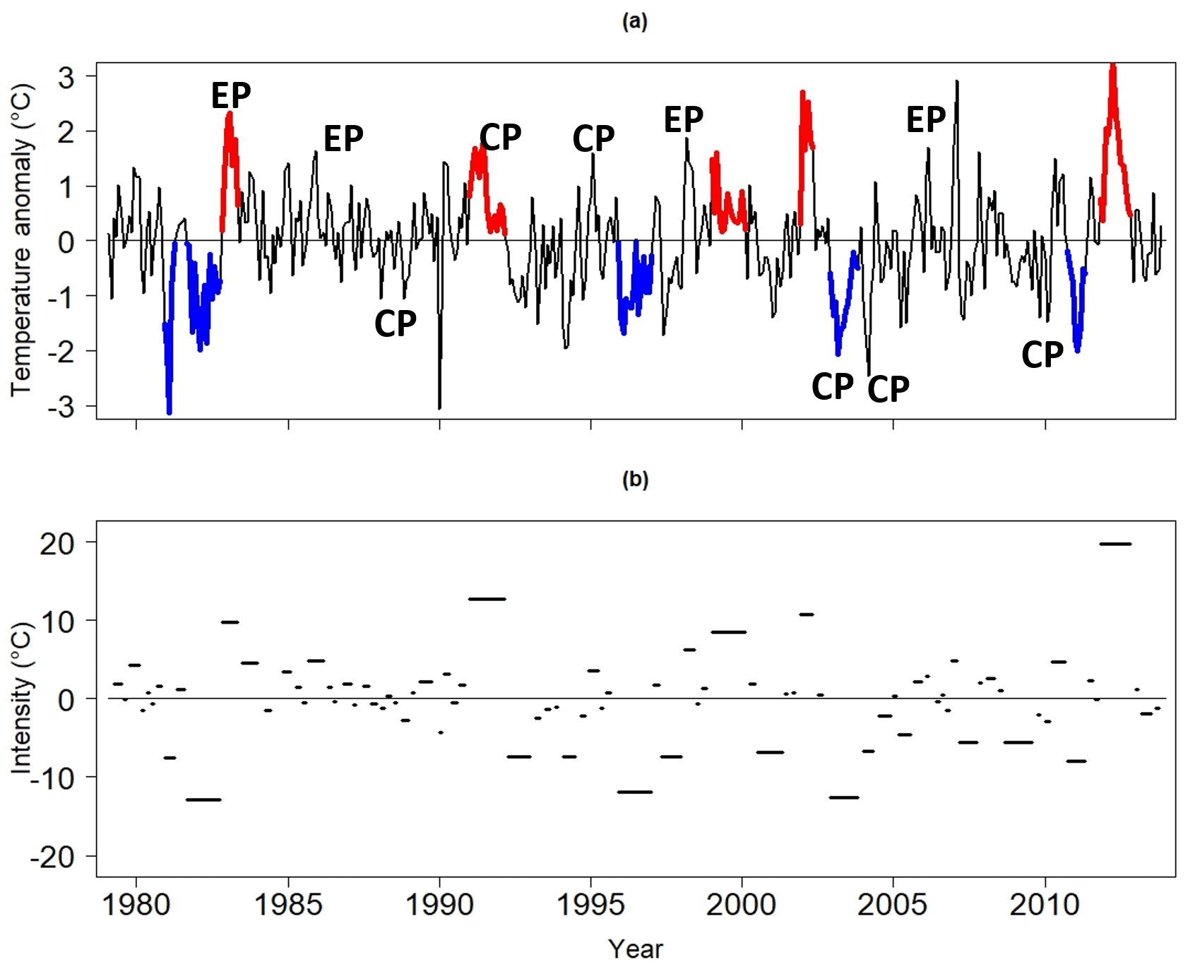
Figure 2(a) The LIS surface temperature anomaly time series and (b) the corresponding event spectrum. Central Pacific El Niño events are indicated by CP and eastern Pacific El Niño events are indicated by EP. Blue curves represent the five most intense negative LIS temperature events, while red curves represent the five most intense positive LIS temperature events. The length of the line segments in (b) represents the persistence of the LIS temperature events. The vertical axis corresponds to the intensity of the event.
4.1 LIS temperature time series
The time series of detrended LIS temperature anomalies is shown in Fig. 2a. Some notable features are the cool periods around 1982, 1996, and 2003 (thick blue lines) and the warm events around 1991, 2001, and 2012. The 1982 cool period is rather intense, with LIS temperature anomalies approaching −2 ∘C. In contrast, the 2012 event is associated with a maximum temperature anomaly of approximately 3 ∘C, making this water temperature anomaly the largest in the 1979–2013 period.
Unlike the simple time series shown in Fig. 2a, the event spectrum shown in Fig. 2b clearly distinguishes the intense LIS events from the weak short-lived events. For example, both the cool period around 1982 and the warm episode around 2012 emerge as the most intense cool and warm events in the 1979–2013 period. The 1996, 2003, and 2011 cold events are nearly as intense as the 1982 event (Table 1). It is interesting to note that the most intense negative events shown in Table 1 peak in winter (December–February). This tendency for negative events to peak in winter was confirmed by computing the number of times a negative event peaked in a given month for a larger set of events (32 events) whose intensities fall below the median of all negative event intensities. A similar but weaker tendency was found for positive events, with a majority of the most intense (greater than 50th percentile) positive events peaking in January and February.
Table 1A total of 10 LIS detrended temperature events ranked by the magnitude of their intensities.
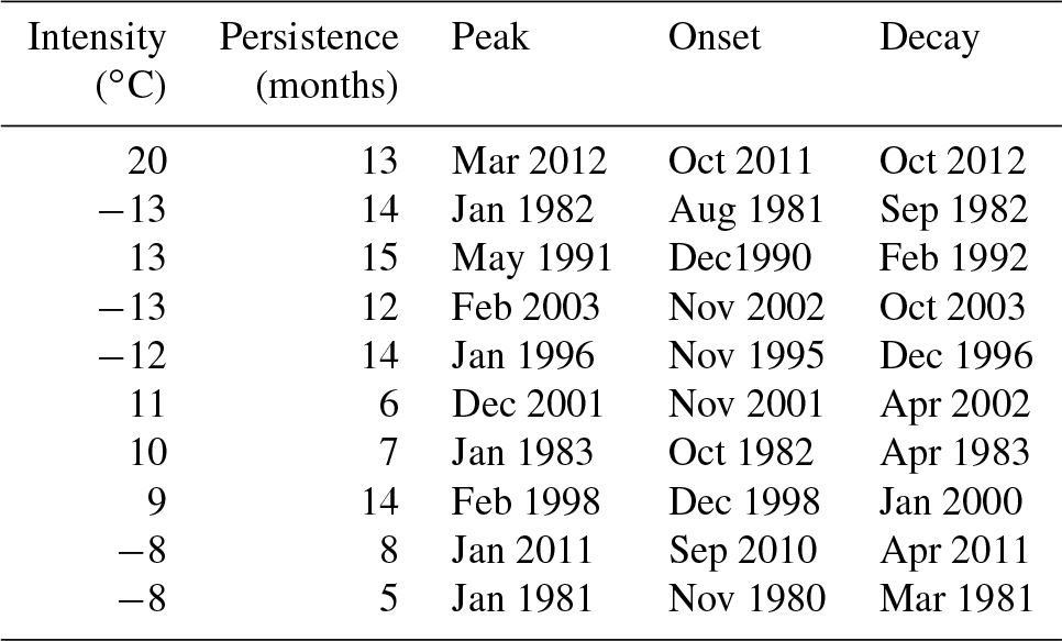
The event spectrum also allows for the clear comparison of event persistence. An inspection of Fig. 2b shows that the intense events are generally more persistent than less intense events. In fact, Table 1 shows that all the most intense events have persistence of at least 5 months, exceeding the average persistence of 3 months calculated using all events. Negative and positive events were found to have similar average persistence. Given that the average persistence is 3 months, the 1982, 1991, 1996, 2003, and 2012 LIS temperature events are unusually persistent compared to other events in the study period. Moreover, not only is the 2012 event among the most persistent, but also its magnitude far exceeds that of any other event even with the removal of the long-term trend. This result suggests that atmospheric variability may have contributed strongly to that event.
4.2 LIS events and atmospheric patterns
To diagnose a possible mechanism behind the occurrence of the intense LIS events, the correlation between 500 hPa geopotential height anomalies and detrended LIS temperature anomalies was computed. We used this one-point correlation approach to extract a relevant teleconnection pattern from a continuum of patterns, much like how the PNA pattern was originally derived (Wallace and Gutzler, 1981). For this analysis, we focused on the December–February (DJF) season because atmospheric circulation anomalies are generally most pronounced during the DJF season and because the peak of events tends to occur in the winter.
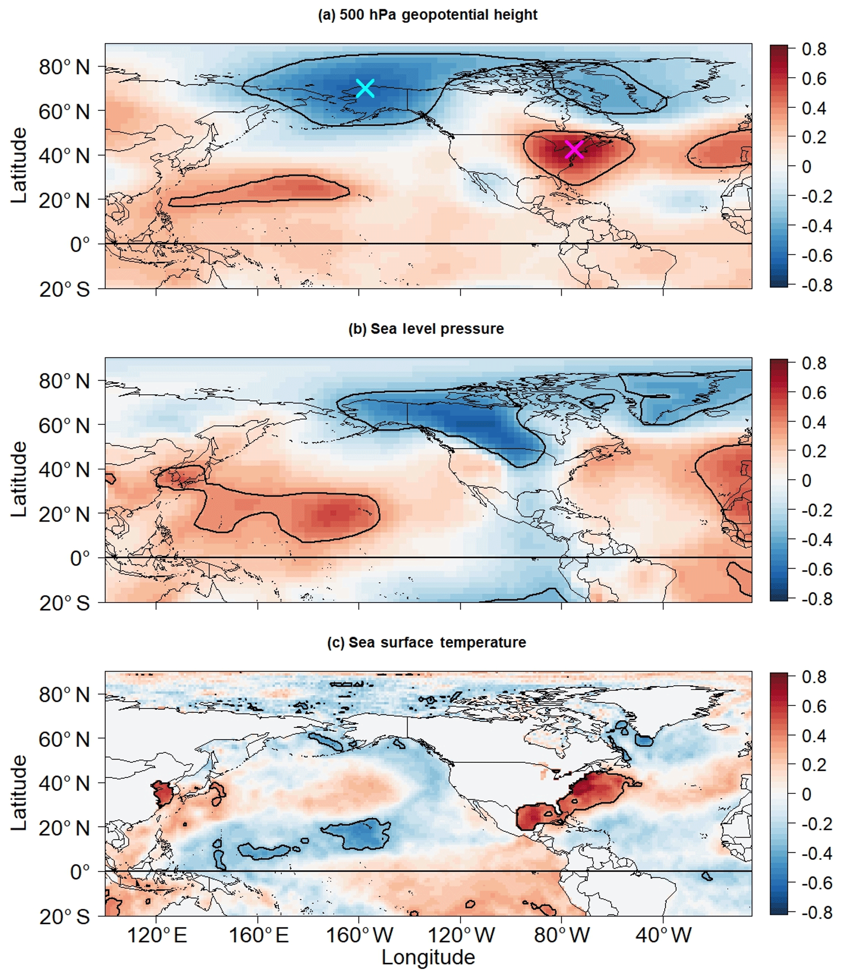
Figure 3Correlation between LIS temperature anomalies and anomalies for (a) DJF 500 hPa geopotential height, (b) SLP, and (c) SST. Contours enclose regions of 5 % statistical significance. Crosses in (a) mark the grid point locations used to construct the dipole index.
Shown in Fig. 3a is the correlation between DJF LIS temperature anomalies and 500 hPa geopotential height anomalies. The positive correlation between LIS temperature anomalies and 500 hPa geopotential height anomalies over the eastern US suggests that warmer-than-normal LIS temperature conditions are associated with a jet stream ridge, which is consistent with how jet stream configurations can influence the temperature in the coastal ocean off the northeastern US (Chen et al., 2014). Similarly, the negative correlations with 500 hPa geopotential height anomalies across Alaska indicate that LIS warm events are associated with an anomalous trough over Alaska. Thus, it appears that LIS temperature events are related to a ridge–trough dipole pattern, an anomalously amplified wave pattern across the US.
For comparison, the 500 hPa geopotential height anomaly field for the March 2012 event is shown in Fig. 4a. Negative 500 hPa geopotential height anomalies are seen across Alaska, and positive 500 hPa geopotential height anomalies are seen across the eastern US and across the central North Pacific. This 500 hPa geopotential height anomaly configuration is consistent with the results presented in Fig. 3a, suggesting that the ridge–trough dipole pattern was an important contributor to the March 2012 LIS temperature event.
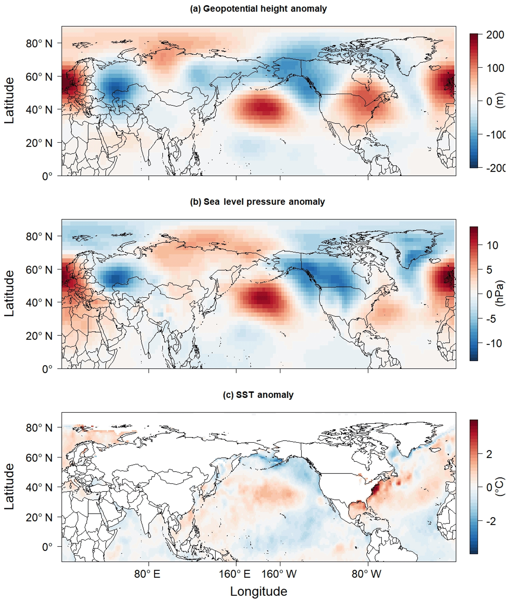
Figure 4Anomalies for (a) 500 hPa geopotential height, (b) SLP, and (c) SST corresponding to the March 2012 LIS temperature event.
A physical mechanism behind the ridge–trough dipole–LIS temperature association was diagnosed by examining the relationship between DJF SLP anomalies and LIS temperature anomalies. As shown in Fig. 3b, DJF LIS temperature anomalies are negatively correlated with DJF SLP anomalies across northwestern Canada. Thus, positive LIS temperature anomalies are associated with anomalous cyclonic flow, whereas negative LIS temperature anomalies are associated with anomalous anticyclonic flow. These relationships are physically consistent with findings from previous works showing how upstream (relative to the LIS) surface anticyclones play a crucial role in the occurrence of cold temperature extremes across the northeast US (Konrad, 1996, 1998). Such surface anticyclones have been shown to be dynamically supported by a ridge–trough wave pattern in the middle troposphere (Konrad, 1998; Jones and Cohen, 2011), in agreement with the results shown in Fig. 3a. At the surface, the anticyclone results in cold advection from a high-latitude source region into the LIS region (Fig. 5a). Cyclones are also typically present along the east coast of the US during cold temperature events (Konrad, 1998), which could explain the positive correlation between LIS temperature anomalies and SLP anomalies along the east coast of the US. Features associated with positive LIS temperature anomalies are opposite to those found for negative LIS temperature anomalies (Fig. 5b).
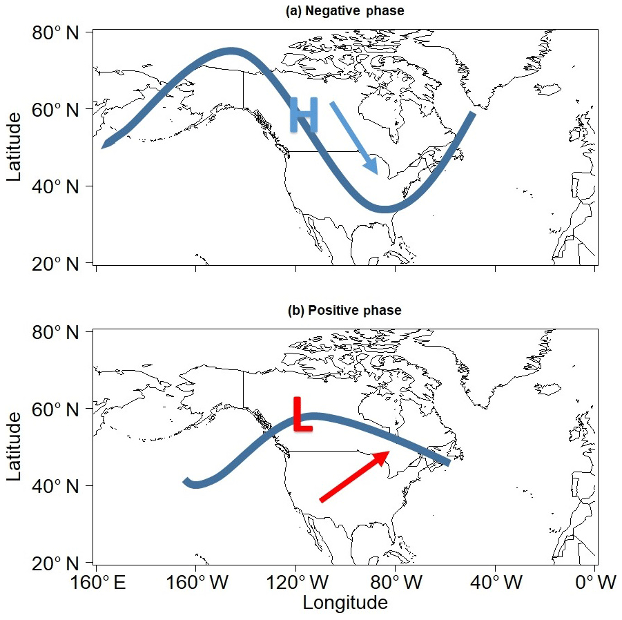
Figure 5(a) Idealized schematic of atmospheric features occurring during negative LIS temperature events and negative phases of the dipole pattern. (b) Same as (a) but for positive LIS temperature events and positive phases of the dipole pattern. Thick blue curves represent the idealized jet stream configuration, while the blue (red) arrow indicates the general movement of cold (warm) air masses. High pressure is indicated with an H and low pressure is indicated with an L.
As a specific example, consider the SLP anomaly pattern for March 2012 (Fig. 4b). Negative SLP anomalies are seen to extend from western Alaska to central Canada, indicative of anomalously strong cyclonic flow and warm air advection across the eastern US. The locations of the negative SLP anomalies generally coincide where SLP anomalies are correlated with LIS temperature anomalies (Fig. 3b), again suggesting that the ridge–trough pattern played an important role in the March 2012 LIS temperature event.
To better understand LIS water temperature variability, a ridge–trough dipole index was created based on the pattern identified in Fig. 3a. The dipole index was constructed by first locating the grid point for which the correlation between LIS temperature and 500 hPa geopotential height anomalies is minimum. This grid point is located at 70∘ N and 157.5∘ W and is marked by a cyan cross in Fig. 3a. Next, the grid point for which the correlation between LIS temperature and 500 hPa geopotential height anomalies is maximum was located. This grid point is located at 42.5∘ N and 75∘ W and is marked with a magenta cross in Fig. 3a. Following Wang et al. (2014), the dipole index for a given month was defined as the 500 hPa geopotential height anomaly at 42.5∘ N and 75∘ W minus the 500 hPa geopotential height anomaly at 70∘ N and 157.5∘ W. Thus, the dipole index measures the intensity of the ridge–trough dipole pattern such that positive phases generally indicate that an anomalously strong ridge over the eastern US is accompanied by an anomalous trough over Alaska. Correlating the dipole index with SLP anomalies (not shown) reveals that negative (positive) phases of the dipole pattern are associated with positive (negative) SLP anomalies across northwestern Canada and cold (warm) air advection to the east of the anomaly center (Fig. 5).
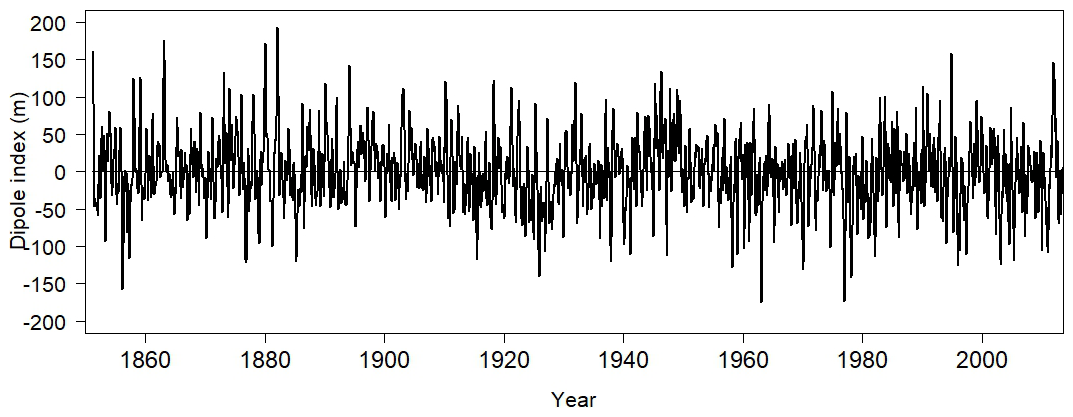
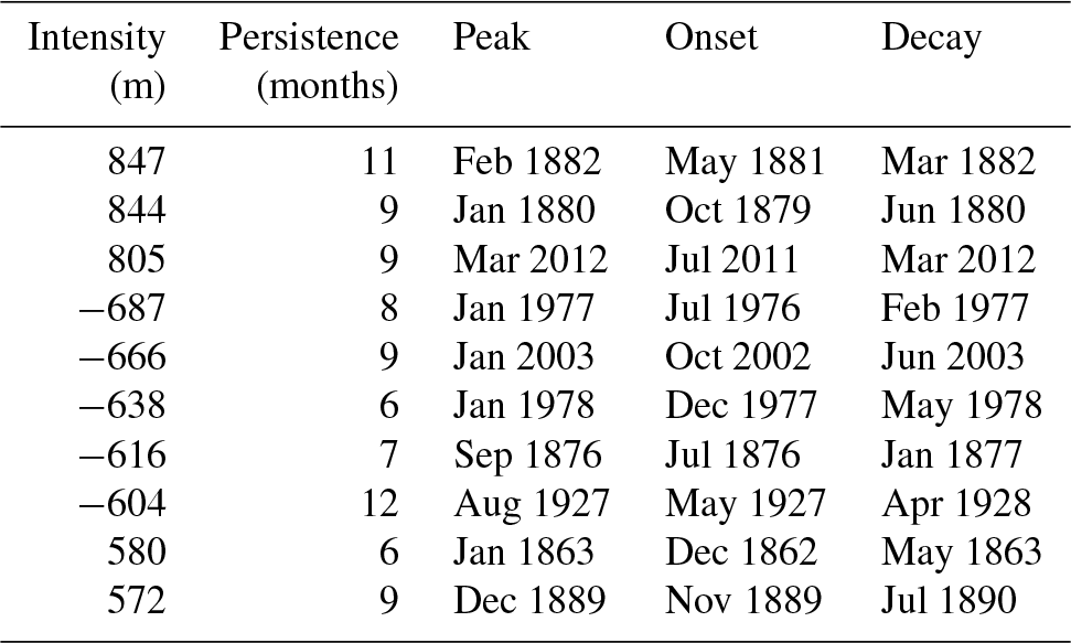
The time series for the 3-month running mean of the dipole index is shown in Fig. 6. The time series is rather noisy, but notable features can still be identified. The dipole pattern, as indicated by positive dipole indices, is seen to be in a persistent positive phase around the 2012 LIS warm event. The positive dipole event around 2012 is quite intense but not as intense as the 1882 positive dipole event that persists for 11 months (Table 2). The most intense negative dipole event occurs around 1977. A comparison of Tables 1 and 2 shows that the second most intense negative dipole event calculated using the raw monthly dipole index time series coincides with the second most intense LIS cold event that occurred around 2003 (Table 1).
Table 2A total of 10 dipole events in the 1851–2013 period ranked by the magnitude of their intensities. Results are based on the raw monthly dipole index time series.
Although a comparison of Tables 1 and 2 shows that the 2012 LIS warm event coincides with the third most intense positive dipole event, the relationship strength between LIS temperature anomalies and the dipole pattern cannot be inferred. How strongly related is the dipole index to LIS water temperature anomalies? To assess the strength of the dipole index relationship with LIS water temperature anomalies, seasonally averaged detrended LIS temperature anomalies were correlated with the seasonally averaged dipole index. As shown in Fig. 7, the dipole index is strongly correlated with LIS temperature anomalies for the October–December (OND), November–January (NDJ), DJF, and January–March (JFM) seasons. The relationships are generally stronger if the dipole index leads by 1 month, as indicated by the dotted line in Fig. 7. The lagged correlation coefficients approach 0.8 for the DJF season, suggesting that DJF LIS temperature anomalies are strongly influenced by the dipole pattern in the NDJ season. Lagged correlations are also strong (r>0.6) for the OND, NDJ, and JFM seasons. The relationships are generally weaker in the warm seasons, possibly because teleconnection patterns are generally of the weakest amplitude in the warm season. Another reason is that LIS temperature anomalies in the winter can persist into the summer (Schulte et al., 2018), weakening the simultaneous relationships between LIS temperature anomalies and the dipole pattern for non-winter seasons. However, the weaker relationships between air temperature and the dipole index in the summer (not shown) likely contribute to the seasonal cycle in relationship strength shown in Fig. 7.
Table 3Correlation between the dipole index and indices for five major climate modes of variability for the 1979–2013 period. Bold entries indicate 5 % statistically significant correlation coefficients.
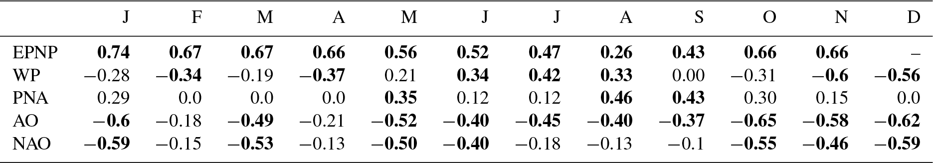
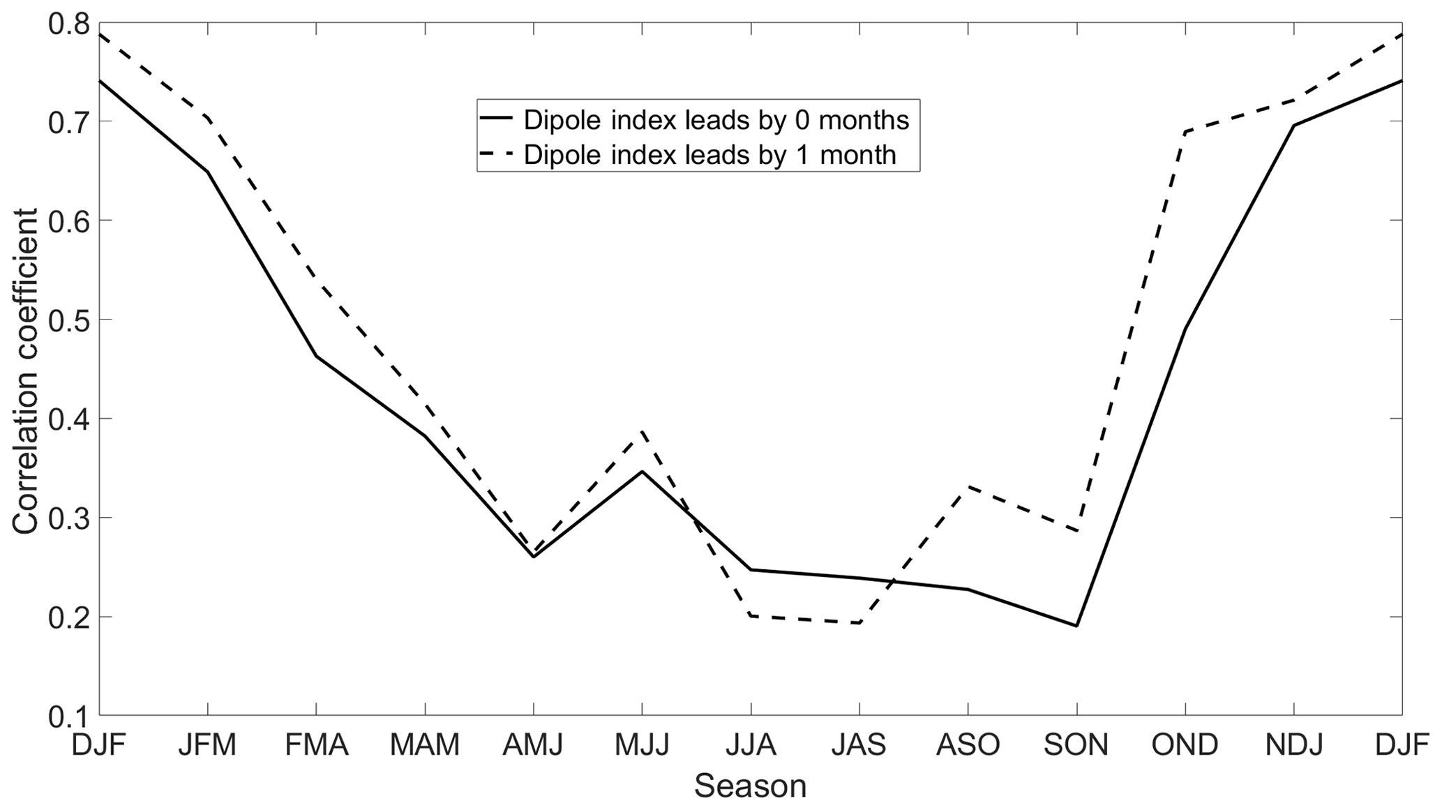
Figure 7Lagged and simultaneous correlations between seasonally averaged LIS water temperature anomalies and the seasonally averaged dipole index. The dotted line represents the correlation between the dipole index of the prior season (dipole leads by 1 month) and water temperature anomalies for the season specified on the horizonal axis.
The relationship strength found between the dipole index and LIS temperature anomalies is consistent with results found in prior work because the dipole index is strongly correlated with the EP–NP index for most months (Table 3) and because the EP–NP index is strongly correlated with LIS temperature anomalies (Schulte et al., 2018). However, Schulte et al. (2018) used an ad hoc approach to construct the December EP–NP index using linear regression. Thus, one may ask the following: is the EP–NP pattern a wintertime pattern? To answer the question, it is first noted that the relationship strength between the EP–NP and dipole indices increases nearly monotonically from August to November, decreases almost monotonically from January to August, and peaks in January. With a such clear seasonal cycle, it is natural to infer that the December dipole pattern is largely the December EP–NP pattern despite how the CPC suggests that the EP–NP pattern is inactive in winter. Because the 500 hPa geopotential height anomaly structure associated with the dipole pattern is the same from November to March (not shown), one can deduce that the December ridge–trough pattern is largely the December EP–NP pattern given the strong relationship between EP–NP and dipole indices during those months. More specifically, we compared the December dipole pattern to the January dipole pattern (Fig. 8) and found them to be similar in terms of 500 hPa geopotential height anomalies. Thus, because the January dipole and EP–NP indices are strongly correlated, the December dipole pattern must also be EP–NP-like. The strong relationships (r>0.8) between air temperature and the dipole pattern in winter suggest that the dipole pattern (or EP–NP pattern) is particularly active in the winter. It also has a strong physical basis because negative phases are associated with 500 hPa western North America and Arctic ridging and eastern US 500 hPa troughing (Fig. 8), all features associated with eastern US cold temperature events (Konrad, 1998). Although Schulte et al. (2018) used the EP–NP index to diagnose historical LIS temperature variability, our dipole index is defined in all months and is easy to calculate, making it more practical in an operational forecasting setting.
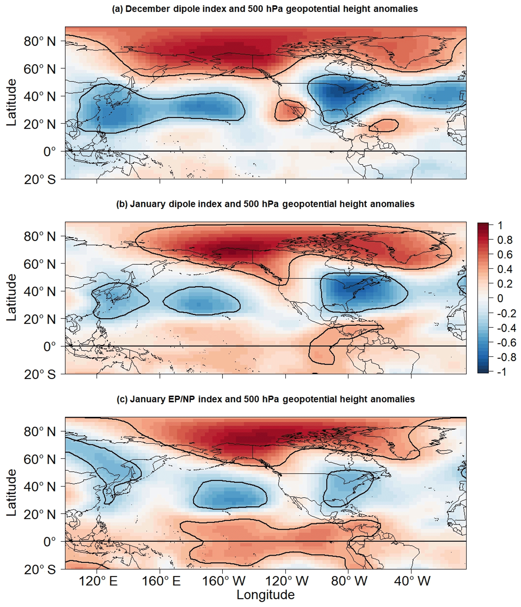
Figure 8Correlation between 500 hPa geopotential height anomalies and indices for the (a) December dipole, (b) January dipole, and (c) January EP–NP patterns. Contours enclose regions of 5 % statistical significance.
While the December dipole index is well correlated with December indices for the AO, NAO, and WP, a close examination of the 500 hPa geopotential height anomaly fields (not shown) associated with those patterns reveals that those patterns are quite different from the dipole pattern found in this study. For example, the NAO and AO indices are correlated with 500 hPa geopotential height around the dipole pattern's eastern center of action (magenta cross in Fig. 3a) but are practically uncorrelated with 500 hPa geopotential height anomalies around the western center of action. The NAO and AO are also much more strongly correlated with 500 hPa geopotential height anomalies across the North Atlantic than the dipole pattern. The WP index is only weakly correlated with 500 hPa geopotential height around both the dipole patterns' centers of actions and much more strongly correlated with 500 hPa geopotential height anomalies across the western North Pacific Ocean. Our results suggest that the reason why the wintertime AO, NAO, and WP patterns are not strongly related with wintertime LIS temperature anomalies as shown by Schulte et al. (2018) is that these patterns are not related to northern Alaskan jet stream ridging, which is important to LIS temperature variability (Fig. 3a).
The fact that the dipole index is correlated with multiple large-scale indices (Table 3) suggests that the dipole pattern falls on a continuum of teleconnection patterns (Franzke and Feldstein, 2005) such that the dipole pattern is strongly EP–NP-like. Although we found by conducting our own EOF analysis of 500 hPa geopotential height anomalies that the AO pattern is the leading mode of variability, the EP–NP pattern appears to be consistently the fifth to seventh leading mode of variability (Table 4). Thus, although the EP–NP pattern is not as dominant as the AO pattern, the dipole pattern tends to more closely resemble it than the AO pattern. Furthermore, the continuum-based extraction of a dipole pattern with a strong relationship to LIS temperature anomalies supports the idea that the continuum approach is useful for understanding climate variability across the northeast US, a finding like that described in previous work focusing on precipitation in the northeast US (Schulte et al. 2017a, b). In particular, our results show that the one-point correlation map approach used by Wallace and Gutzler (1981) is a powerful but simple tool for understanding regional climate variability.
Given that LIS water temperature is strongly correlated with air temperature (Schulte et al., 2018), it is hypothesized that the dipole index is related to air temperature across the US, especially around the LIS. To confirm a dipole index–air temperature relationship, the dipole index was correlated with average monthly air temperature anomalies for the 1979–2013 period (Fig. 9). The results for the NDJ season are only displayed because the strongest correlation found in Fig. 7 is between the NDJ dipole index and DJF LIS water temperature anomalies.
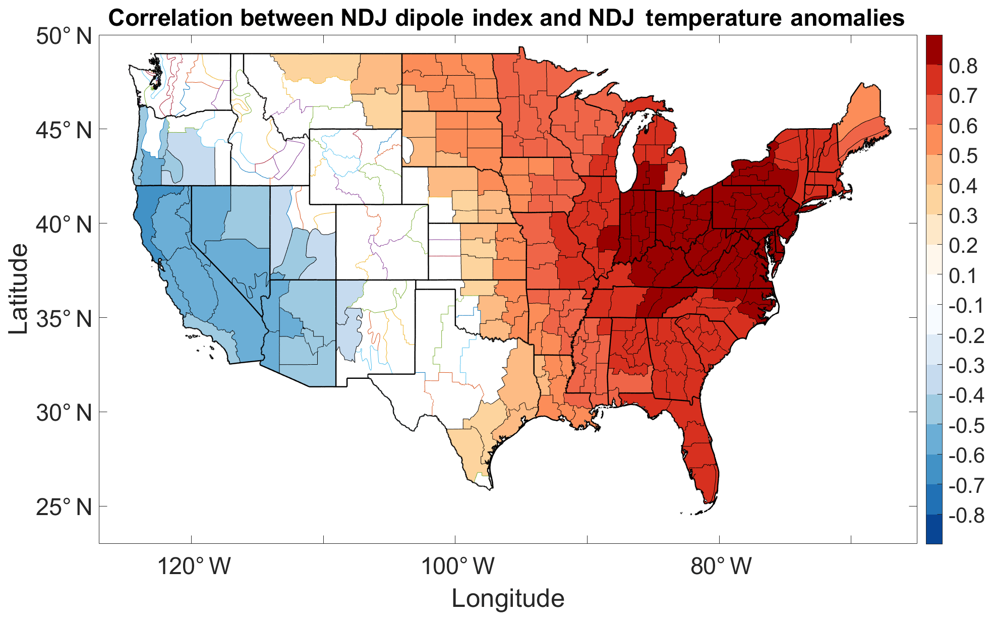
Figure 9Correlation between the NDJ dipole index and NDJ temperature anomalies. Shaded climate divisions are those for which the corresponding correlation coefficients are statistically significant at the 5 % significance level.
As shown in Fig. 9, the dipole index is indeed strongly correlated with air temperature anomalies across a large region of the US. Correlation coefficients exceed 0.8 and approach 0.9 across the northeast US and LIS region. The strong relationships extend to the southern US, and the relationships generally weaken equatorward. The relationships displayed in Fig. 9 are generally stronger than those associated with the AO and NAO (not shown) whose influence on eastern US temperature has been well studied (Hurrell and van Loon, 1997; Wettstein and Mearns, 2002). Thus, our dipole index is useful for diagnostic studies of cold outbreaks across the eastern US. The results for the other seasons are similar, but the relationships for seasons not comprising November, December, January, or February (e.g., June–August) are generally weaker than those identified for the NDJ season. This result suggests that the dipole pattern is rather dominant in the winter. The strong relationship between the dipole index and US air temperature anomalies is consistent with the intense 2012 dipole event coinciding with the record warm March in 2012 (Dole et al., 2014), which resulted in a so-called false spring in which plants bloomed prematurely, making them susceptible to drought and freezes (Ault, 2013). The results shown in Fig. 9 suggest that the dipole pattern's impact on LIS temperature is related to the dipole pattern's influence on air temperature.
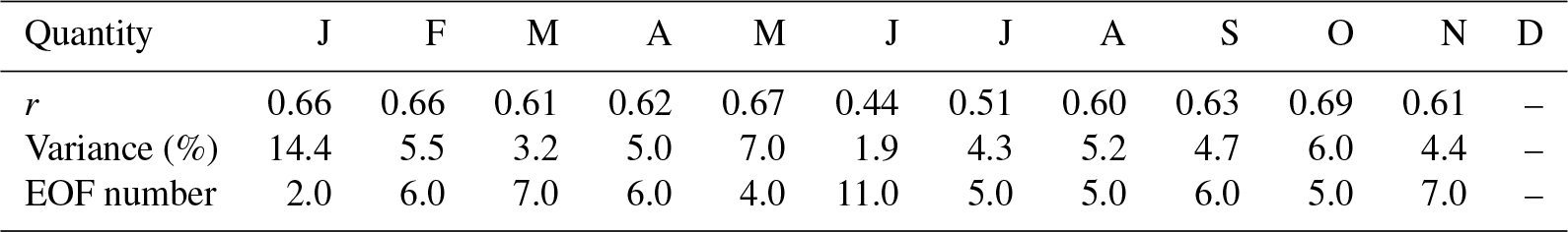
Table 4The mode number of the EOF pattern that most closely resembles the EP–NP pattern, the explained variance associated with the EOF pattern, and the correlation coefficient, r, computed between the corresponding principal component time series and the EP–NP index. The EOF pattern that most closely resembles the EP–NP pattern was determined by finding the EOF pattern whose principal component time series is most strongly correlated with the EP–NP index. The results are based on NCEP reanalysis for the 1979–2013 period.
4.3 Intense LIS events and SST patterns
SST patterns are often used in seasonal forecasting, and thus identifying an SST pattern precursor to LIS temperature events has implications for seasonal prediction of LIS temperature anomalies. To identify SST patterns associated with LIS temperature events, a lagged SST composite analysis was conducted using detrended LIS warm and cool events separately. The SST composite plots for the warm events were constructed using the LIS warm events whose intensities are greater than or equal to the 50th percentile of all warm event intensities (32 events). Similarly, the SST composite plots for the cold events were constructed using LIS cold events whose intensities are less than or equal to the 50th percentile of all LIS cold event intensities (32 events). The composite mean SST patterns were computed at the onset, mature, and decay phases of the LIS events. Because intense LIS events tend to peak in winter, the composite plots for mature phases mainly reflect wintertime conditions.

Figure 10Composite mean SST anomalies corresponding to (a) onset, (b) mature, and (c) decay phases of negative LIS temperature events. Contours enclose regions of 5 % statistical significance, as determined by a one sample t test.
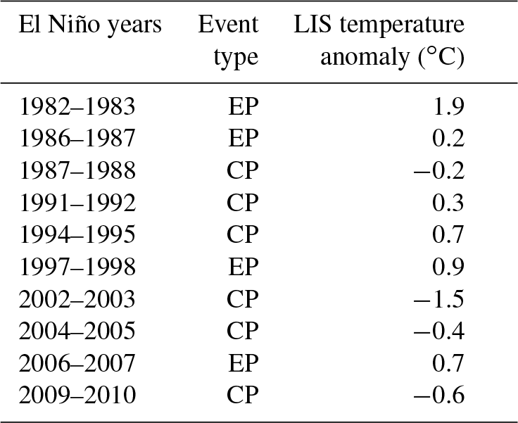
The results for the LIS cold events are shown in Fig. 10. The composite plot shown in Fig. 10a indicates that the onset of LIS cold events is associated with positive SST anomalies across the central equatorial Pacific. The results suggest that LIS cold events could be initiated by central Pacific El Niño events (Lee and McPhaden, 2010). A few examples of central Pacific El Niño events (based on the December–March season) are the 1991–1992, 1994–1995, 2002–2003, 2004–2005, and 2009–2010 events (Table 5), but a more complete list can be found in Johnson and Kosaka (2016). The 2002–2003, 2004–2005, and 2009–2010 events all appear to occur around LIS cold periods (Fig. 2a). Note that there could be lags between the onset of central Pacific El Niños and LIS temperature anomalies because of the lagged response of water temperature to atmospheric forcing (Schulte et al., 2018). In addition, preexisting positive water temperature anomalies may need time to degrade.
Table 5El Niño events partitioned into central (CP) and eastern (EP) Pacific types based on the categorization method of Yu et al. (2012). El Niño events are defined based on the DJFM season. The third column provides the corresponding DJFM LIS temperature anomaly. A more complete table of El Niño events can be found in Johnson and Kosoka (2016).
The SST anomaly pattern for the mature phases of LIS cold events features positive SST anomalies across the central equatorial Pacific (Fig. 10b). However, the mature-phase composite mean SST anomaly pattern is more pronounced across the North Pacific Ocean than it is for the onset phase. A region of positive SST anomalies is seen to be horseshoe-shaped, with positive SST anomalies extending from the central equatorial Pacific to the US west coast. Although Hartmann (2015) found an SST pattern resembling that shown in Fig. 9b to be a contributor to the February 2015 eastern US cold event, only a single event was considered. In this study, we show that the pattern is associated with numerous LIS negative temperature events (and thus eastern US air temperature events), many of which persist for more than 5 months. Thus, we show here that the SST pattern influences both the intensity and persistence of events. It is noted that the pattern shown in Fig. 10b resembles the DJF SST pattern of 1996, which is consistent with 1996 being a cooler-than-normal period for much of the US (Halpert and Bell, 1997) and the LIS (Table 1).
Unlike the composite mean SST pattern corresponding to the onset phase, negative SST anomalies are present along the US east coast and across the Gulf of Mexico during mature phases. These results are consistent with LIS temperature anomalies being strongly associated with the dipole pattern that influences air temperature across regions adjacent to the Gulf of Mexico and US east coast. This relationship between the dipole index and SST anomalies was confirmed by correlating the dipole index with SST anomalies for different seasons (not shown).
The tropical SST pattern associated with the decay phase of LIS cold events is different from those associated with the onset and mature phases (Fig. 10c). The composite mean SST anomaly pattern most closely resembles the first leading mode of SST variability called the canonical ENSO pattern (Hartmann, 2015), though the most intense positive SST anomalies are still confined to the central equatorial Pacific. This result suggests that there may be a tendency for the decay of LIS cold events to coincide with canonical ENSO patterns or an SST pattern that is a mixture of central and eastern Pacific El Niño flavors lying on a continuum of ENSO flavors (Johnson, 2013).
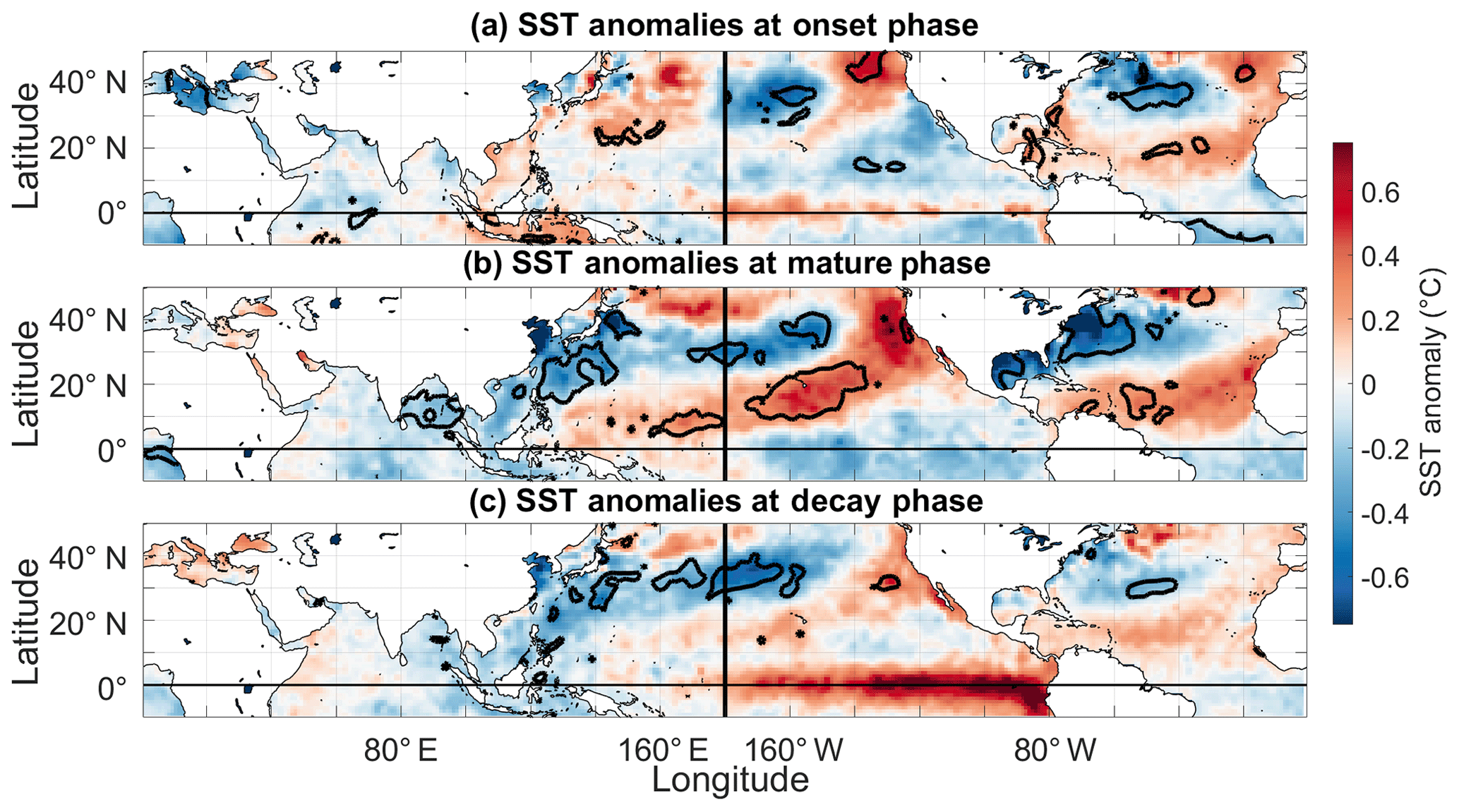
Figure 11Same as Fig. 10 but using the criterion that the intensities of the negative LIS temperature events fall below the 10th percentile of negative LIS temperature event intensities.
The tendency for the decay of LIS cold events to coincide with canonical ENSO patterns is more evident when constructing SST composites using the 10th percentile (Fig. 11) instead of the 50th percentile used to construct the composite shown in Fig. 10. However, possibly because of small sample sizes (seven events), the results generally lack statistical significance. Nonetheless, the event spectrum depicted in Fig. 2b indicates that the major cool periods around 1982 and 1997, for example, terminate around the major 1982–1983 (Ramusson and Wallace, 1983; Quiroz, 1983) and 1997–1998 (McPhaden, 1999) El Niño events. Although Schulte et al. (2018) showed that LIS temperature anomalies are associated with a single SST pattern, we show in this study that predicting the evolution of LIS temperature events may require knowledge of several ENSO flavors.
The SST pattern across the Atlantic Ocean shown in Fig. 11 resembles a well-documented North Atlantic tripole mode (Deser and Blackmon, 1993; Fan and Schneider, 2011), which comprises three anomaly centers, one located off the southeastern US coast, a second one located east of Newfoundland, and a third one located in the tropical east Atlantic. This tripolar SST mode has been shown to be related to ENSO, the NAO, and local wind forcing (Fan and Schneider, 2011). The association between the tripole pattern and the LIS water temperature could reflect weak influences of the NAO on LIS water temperature. This interpretation is consistent with the NAO and dipole patterns being related in the winter (Table 3). However, these Atlantic SST anomalies generally lack statistical significance, and this finding is consistent with the LIS water temperature anomalies being only weakly related to the NAO.
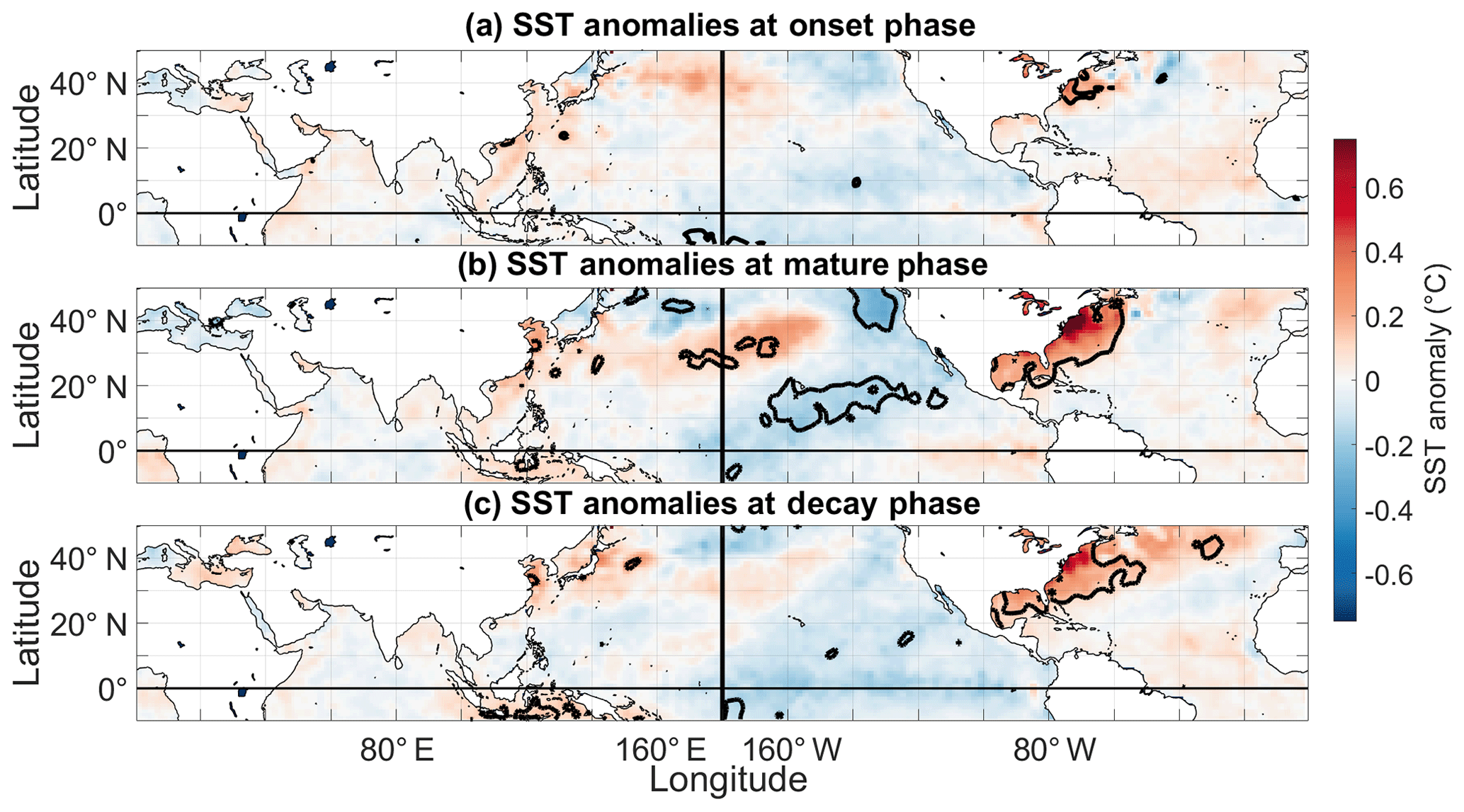
The composite analysis was also conducted for LIS warm events, and the results revealed that LIS warm events are also associated with SST modes of variability (Fig. 12). The onset of LIS warm events appears not to be associated with any coherent SST pattern. For the mature phase, statistically significant negative SST anomalies are seen across the central equatorial Pacific and positive SST anomalies are seen across the eastern equatorial Pacific. Like the SST anomaly pattern associated with mature phases of LIS cold events (Figs. 10b and 11b), the pattern shown in Fig. 12b generally resembles the third leading mode of SST variability (Hartman, 2015). The SST pattern corresponds well to the SST anomaly pattern associated with March 2012 (Fig. 4c), a month in which record warmth was experienced across the central and eastern US (Dole et al., 2014). Mature phases are also associated with positive SST anomalies along the US east coast and across the Gulf of Mexico like March 2012 (Fig. 4c). Decay phases (Fig. 12c) appear to be associated with negative SST anomalies across the eastern and central equatorial Pacific, but the results were not found to be statistically significant.
The warm LIS events were found to be sensitive to the threshold used to construct the composites. For example, if we only considered the LIS warm events whose intensities were greater than or equal to the 90th percentile of LIS warm event intensities, then all phases of LIS warm events would resemble the pattern shown in Fig. 12b. In general, the positive SST anomalies across the eastern Pacific were found to become more intense as the percentile used to establish the threshold was increased from 50 to 90. Despite the lack of statistical significance in the composite plots, statistically significant relationships with SST anomalies were found when correlating DJF LIS temperature anomalies with DJF SST anomalies (Fig. 3c). The identified correlation pattern was found to resemble the pattern shown in Figs. 10b and 11b.
The SST composite analyses were also conducted using the dipole events for the 1979–2013, 1950–2013, and 1870–2013 periods. The resulting SST patterns were found to be like those shown in Figs. 10, 11, and 12, which is not surprising given the strong correlation between the dipole index and LIS temperature anomalies. Thus, intense long-lived dipole patterns seem to have a tropical origin, suggesting that a key to better understanding LIS temperature events rests in a firmer understanding of tropical processes.
4.4 Decadal variability
The results of the composite analyses suggest that dipole events may be associated with tropical SST patterns, but the timescale at which the SST patterns are most strongly associated with the dipole pattern cannot be inferred from the analysis. Thus, a wavelet coherence analysis was conducted to determine if the SST modes fluctuate coherently with the dipole pattern at a preferred timescale. The wavelet squared coherence was computed between the dipole index and indices for the Niño 3 and Niño 4 metrics, but the results using the Niño 4 index were found to be most robust. As such, the results for the Niño 4 index analysis only are shown.
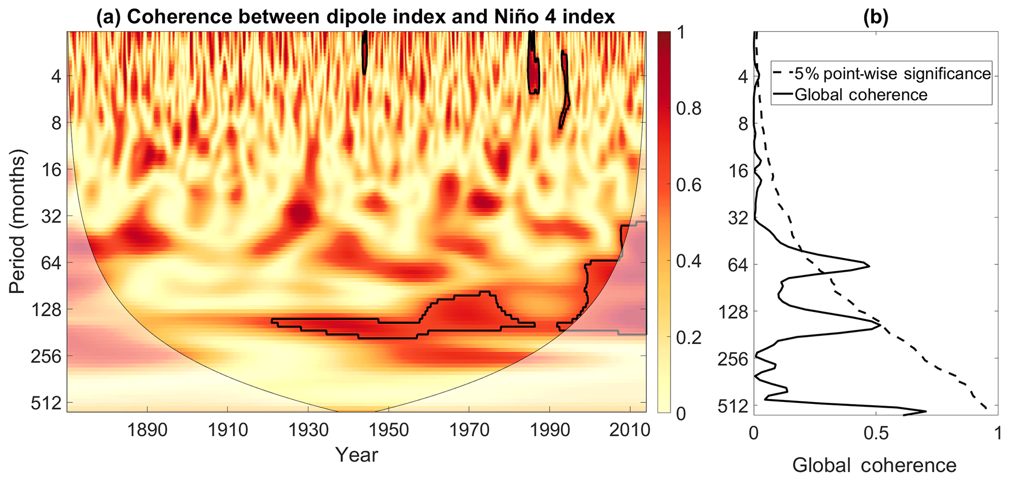
Figure 13(a) Wavelet coherence between the dipole and Niño 4 indices. Contours enclose regions of 5 % cumulative area-wise significance. (b) The global coherence spectrum corresponding to (a). Dotted line is the 5 % point-wise significance bound and the red curves indicate 5 % arc-wise significant coherence values.
The results shown in Fig. 13a indicate that the dipole and Niño 4 indices fluctuate coherently in the 64- to 256-month period after 1930. The results suggest that stronger decadal-scale fluctuations in central equatorial Pacific SSTs are associated with larger decadal fluctuations in the dipole pattern. Given that the decadal-scale fluctuations in the dipole pattern contribute to the overall variance of the dipole index around 2012, the decadal-scale fluctuations must contribute to some extent to the intense dipole event of 2012. The results from the coherence analysis thus suggest that central equatorial Pacific SST fluctuations may have contributed to that intense dipole event.
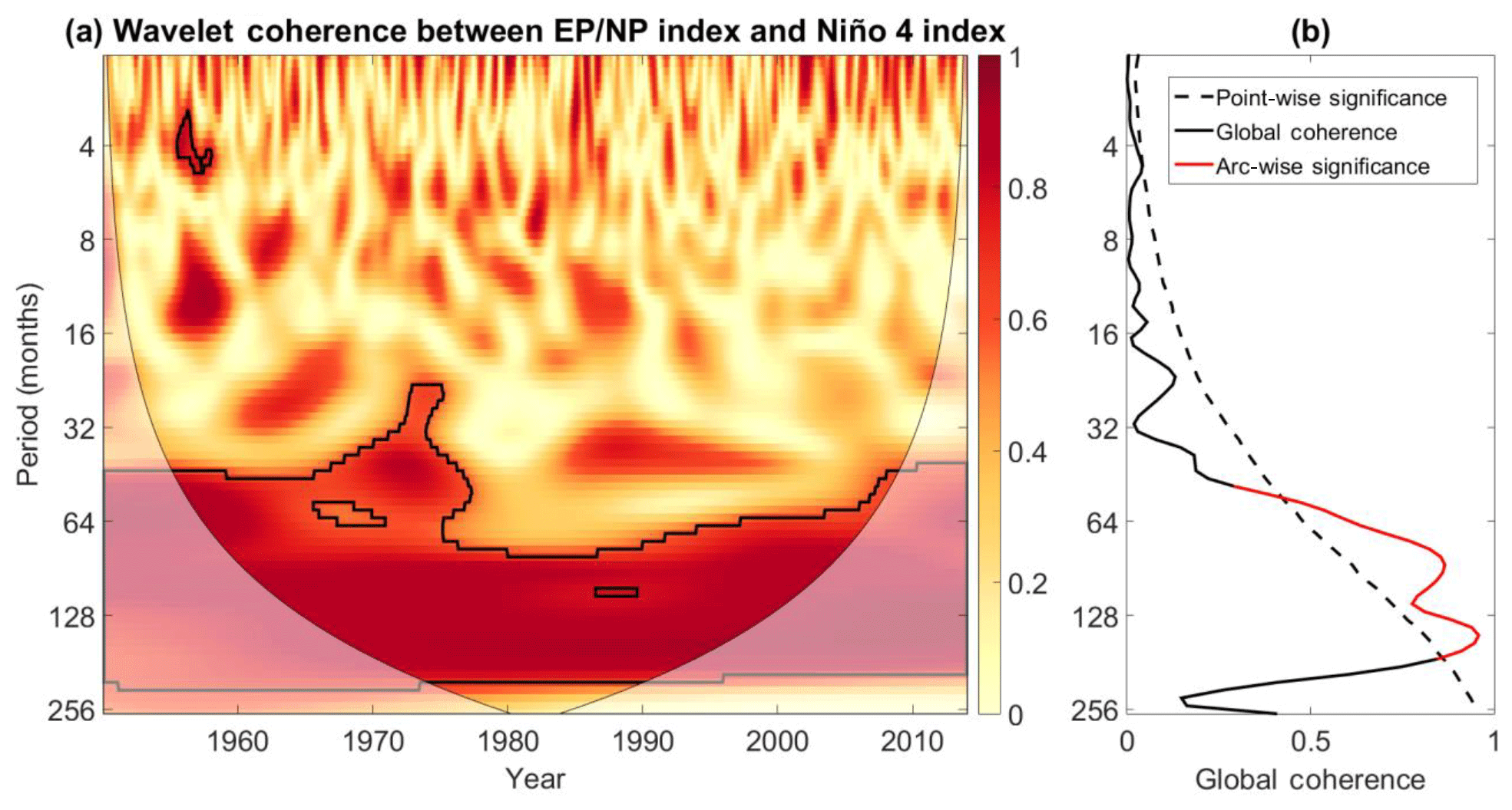
Figure 14Same as Fig. 13 but for the wavelet coherence between the EP–NP and Niño 4 indices.
The strong correlation between the EP–NP and dipole indices (Table 3) suggests that the coherence between the EP–NP and Niño 4 indices is also strong. The strong coherence was confirmed by computing the wavelet squared coherence between the EP–NP and Niño 4 indices for the 1950–2013 period. To perform the analysis, the missing values for the EP–NP index in December were filled by establishing a linear relationship between the EP–NP and dipole indices for all months but December. The linear relationship was obtained using a least-squares fit of a line, and it was used to fill missing EP–NP values based on the available December dipole index values.
As shown in Fig. 14, the EP–NP index does indeed fluctuate coherently with the Niño 4 index. The coherence appears to be strong, and the global coherence spectrum shows arc-wise significant global wavelet coherence in the 64–256 month period. As shown by Schulte et al. (2018), the EP–NP pattern fluctuates strongly on quasi-decadal timescales, but no possible source of the variability was identified. We show in Fig. 14 that the EP–NP variability on quasi-decadal timescales may be related to quasi-decadal fluctuations in central equatorial Pacific SSTs. Because the EP–NP pattern fluctuates coherently with LIS water temperature on decadal timescales (Schulte et al., 2018), LIS water temperature should also fluctuate coherently with the Niño 4 index, though the LIS temperature time series is too short to draw strong conclusions.
This paper revealed that LIS events are associated with modes of tropical Pacific and North Pacific SST variability. The phases of the LIS events were found to depend on the spatial characteristics of the SST patterns. The onset of LIS cold events was shown to be associated with central equatorial Pacific SST anomalies, whereas the decay phase of such events was shown to coincide with canonical ENSO events. These results suggest that central Pacific El Niño events can be used to construct outlooks for the onset of major LIS cold events. Similarly, information regarding the formation of canonical ENSO events could prove useful as guidance for assessing how likely it is that an LIS cold event will end. Conversely, major LIS cold events could be used to anticipate the formation of El Niño events.
The strong relationships identified between the dipole index and LIS temperature anomalies suggest that the dipole index should be incorporated into LIS temperature outlooks and possibly temperature outlooks for other regions of the US as well. The forecast skill associated with such outlooks will depend on the ability to predict the phase and intensity of the dipole pattern. The association between tropical SST patterns and the dipole pattern could prove useful in extended dipole pattern outlooks, contrasting with the AO index whose predictability is limited (Jung et al., 2011). The coherence between the Niño 4 index and indices for the EP–NP and dipole patterns supports the idea that extended dipole pattern outlooks based on tropical SST patterns may be possible. More research, however, is needed to quantify the ability of dynamical weather and seasonal forecasting models to predict the pattern.
Although not the focus of this paper, the dipole pattern may be an important temperature indicator for other estuaries across the northeast US. The correlation pattern shown in Fig. 9 suggests that the dipole pattern could be an important temperature indicator for the Delaware Bay and Chesapeake Bay estuaries. The strong correlation between air temperature and the dipole index across Maine also suggests that the dipole pattern may contribute significantly to the variability of water temperature across the Gulf of Maine. The Gulf of Maine has experienced rapid warming during the past decade (Pershing et al., 2015) and understanding the causes of the rapid warming has important implications for fisheries. Future work could therefore include understanding how the dipole pattern may have contributed to the rapid Gulf of Maine warming.
The results from the present analysis are consistent with temperature events that occurred after the study period considered in this study. For example, the cold period around February 2015 transitioned into a record warm period for most of the US. The record warm period lasting from September 2015 to December 2015 coincided with an extreme El Niño event (Hu and Federov, 2017). In agreement with our results, the February 2015 SST pattern strongly resembled the SST pattern shown in Fig. 10b, which our results suggest occurs at the peak of LIS cold events. Furthermore, the SST pattern and extreme cold across the eastern US occurred before the El Niño formation, which is also in agreement with the results from the present study. These recent events support the results from our study, which indicate that extended LIS temperature outlooks may be possible if information regarding ENSO flavors is incorporated into such outlooks.
The 20th century reanalysis data are available at https://www.esrl.noaa.gov/psd/data/20thC_Rean/ (NOAA/OAR/ESRL PSD, last access: 6 September 2015) and NCEP reanalysis data are available at https://www.esrl.noaa.gov/psd/data/gridded/data.ncep.reanalysis.html (NOAA/OAR/ESRL PSD, last access: 29 May 2016). The Hadley SST data are available at https://www.metoffice.gov.uk/hadobs/hadisst/data/download.html (MOHC, last access: 15 June 2017). Monthly indices for the atmospheric climate modes can be found at https://www.esrl.noaa.gov/psd/data/climateindices/list/ (NOAA/OAR/ESRL PSD, last access: 15 November 2018), while the long-term Niño 3.4 and Niño 4 indices are available at https://www.esrl.noaa.gov/psd/gcos_wgsp/Timeseries/ (last access: 15 November 2018). The Long Island Sound data are available at https://www.researchgate.net/publication/306256135_LIS_tmp_8113 (last access: 1 September 2015, Georgas et al., 2015). The dipole index and forecasting tools are available at http://justinschulte.com/forecasting/dipole.html (Schulte, 2018, last access: last access: 7 April 2018).
JS conceived the idea for the analysis and also conducted the analyses. SL provided guidance and expertise for the analyses and the preparation of the paper.
The authors declare that they have no conflict of interest.
This study was partially funded by the
National Science Foundation (award number: AGS-1822015).
Edited by: Mario Hoppema
Reviewed by: two
anonymous referees
Ault, T. R, Henebry, G. M., de Beurs, K. M., Schwartz, M. D., Betancourt, J. L., and Moore, D.: The false spring of 2012, earliest in North American record, Eos, T. Am. Geophys. Union, 94, 181–182, https://doi.org/10.1002/2013EO200001, 2013.
Barnston, A. and Livezey, R. E.: Classification, seasonality, and persistence of low-frequency circulation patterns, Mon. Weather Rev., 115, 1083–1126, 1987.
Chen, K., Gawarkiewicz, G. G., Lentz, S. J., and Bane, J. M.: Diagnosing the warming of the Northeastern US Coastal Ocean in 2012: A linkage between the atmospheric jet stream variability and ocean response, J. Geophys. Res.-Ocean., 119, 218–227, https://doi.org/10.1002/2013JC009393, 2014.
Collie, J. S., Wood, A. D., and Jeffries, H. P: Long-term shifts in the species composition of a coastal fish community, Can. J. Fish. Aquat. Sci., 65, 1352–1365, 2008.
Compo, G. P., Whitaker, J. S., Sardeshmukh, P. D., Matsui, N., Allan, R. J, Yin, X., Gleason, B. E., Vose, R. S., Rutledge, G., Bessemoulin, P., Brönnimann, S., Brunet, M., Crouthamel, R. I., Grant, A. N., Groisman, P. Y., Jones, P. D., Kruk, M., Kruger, A. C., Marshall, G. J., Maugeri, M., Mok, H. Y., Nordli, Ø., Ross, T. F., Trigo, R. M., Wang, X. L., Woodruff, S. D., and Worley, S. J.: The Twentieth Century Reanalysis Project, Q. J. Roy. Meteor. Soc., 137, 1–28, https://doi.org/10.1002/qj.776, 2011.
Deser, C. and Blackmon, M. L.: Surface climate variations over the North Atlantic Ocean during winter: 1900–1989, J. Clim., 6, 1743–1753, 1993.
Di Lorenzo, E., Schneider, N., Cobb, K. M., Franks, P. J. S., Chhak, K., Miller, A. J., McWilliams, J. C., Bograd, S. J., Arango, H., Curchitser, E., Powell, T. M., and Rivière, P.: North Pacific Gyre Oscillation links ocean climate and ecosystem change, Geophys. Res. Lett., 35, L08607, https://doi.org/10.1029/2007GL032838, 2008.
Dole, R., Hoerling, M., Kumar, A., Eischeid, J., Perlwitz, J., Quan, X.-W., Kiladis, G., Webb, R., Murray, D., Chen. M., Wolter, K., and Zhang, T.: The making of an extreme event: Putting the pieces together, B. Am. Meteorol. Soc., 95, 427–440, 2014.
Fan, M. and Schneider, E. K.: Observed decadal North Atlantic tripole SST variability, Part I: Weather noise forcing and coupled response, J. Atmos. Sci., 69, 35–50, https://doi.org/10.1175/JAS-D-11-018.1, 2011.
Franzke, C. and Feldstein, S. B.: The continuum and dynamics of Northern Hemisphere teleconnection patterns, J. Atmos. Sci., 62, 3250–3267, 2005.
Georgas, N., Yin, L., Jiang, Y., Wang, Y., Howell, P., Saba, V., Schulte, J., Orton, P., and Wen, B.: An open-access, multi-decadal, three-dimensional, hydrodynamic hindcast dataset for the Long Island Sound and New York/New Jersey Harbor Estuaries, available at: https://www.researchgate.net/publication/306256135_LIS_tmp_8113, last access: 1 September 2015.
Georgas, N., Yin, L., Jiang, Y., Wang, Y., Howell, P., Saba, V., Schulte, J., Orton, P., and Wen, B.: An open-access, multi-decadal, three-dimensional, hydrodynamic hindcast dataset for the Long Island Sound and New York/New Jersey Harbor Estuaries, J. Mar. Sci. Eng., 4, 1–22, 2016.
Grinsted, A., Moore, J. C., and Jevrejeva, S.: Application of the cross wavelet transform and wavelet coherence to geophysical time-series, Nonlin. Process. Geophys., 11, 561–566, 2004.
Guttman, N. and Quayle, R.: A historical perspective of US climate divisions, B. Am. Meteorol. Soc., 77, 293–303, 1996.
Hadley Centre for Climate Prediction and Research/Met Office/Ministry of Defence/United Kingdom: updated monthly, Hadley Centre Global Sea Ice and Sea Surface Temperature (HadISST), Research Data Archive at the National Center for Atmospheric Research, Computational and Information Systems Laboratory, available at: http://rda.ucar.edu/datasets/ds277.3/ (last access: 12 October 2017), 2000.
Halpert, M. and Bell, G.: Climate assessment for 1996, B. Am. Meteorol. Soc., 78, S1–S49, 1997.
Hartmann, D. L.: Pacific Sea Surface Temperature and the Winter of 2014, Geophys. Res. Lett., 42, 1894–1902, 2015.
Howell, P. and Auster, P.: Phase shift in an estuarine finfish community associated with warming temperatures, Mar. Coast. Fish. Dyn. Manag. Ecosyst. Sci., 4, 481–495, 2012.
Hu, S. and Fedorov, A. V.: The extreme El Nino of 2015–2016 and the end of global warming hiatus, Geophys. Res. Lett., 44, 3816–3824, 2017.
Hurrell, J. W.: Decadal trends in the North Atlantic Oscillation regional temperatures and precipitation, Science, 269, 676–679, 1995.
Hurrel, J. W. and H. van Loon: Decadal variations in climate associated with the North Atlantic Oscillation, Climatic Change, 36, 301– 326, 1997.
Johnson, N. C.: How Many ENSO Flavors Can We Distinguish?, J. Clim., 26, 4816–4827, 2013.
Johnson, N. C. and Feldstein, S. B.: The continuum of North Pacific sea level pressure patterns: Intraseasonal, interannual, and interdecadal variability, J. Clim., 23, 851–867, 2010.
Johnson, N. C., Feldstein, S. B., and Tremblay, B.: The continuum of Northern Hemisphere teleconnection patterns and a description of the NAO shift with the use of self-organizing maps, J. Clim., 21, 6354–6371, 2008.
Johnson, N. C and Kosaka, Y.: The role of eastern equatorial Pacific convection on the diversity of boreal winter El Niño teleconnection patterns, Clim. Dynam., 47, 3737–3765, 2016.
Jones, J. E. and Cohen, J.: A diagnostic comparison of Alaskan and Siberian strong anticyclones, J. Clim., 24, 2599–2611, 2011.
Jung, T., Vitart, F., Ferranti, L., and Morcrette, J.-J.: Origin and pre-dictability of the extreme negative NAO winter of 2009/10, Geophys. Res. Lett., 38, L07701, https://doi.org/10.1029/2011GL046786, 2011.
Kalnay, E., Kanamitsu, M., Kistler, R., Collins, W., Deaven, D., Gandin, L., Iredell, M., Saha, S., White, G., Wollen, J., Zhu, Y., Chelliah, M., Ebisuzaki, W., Higgins, W., Janowiak, J., Mo, K.C., Ropelewski, C., Wang, J., Leetmaa, A., Reynolds, R., Jenne, R., and Joseph, D.: The NCEP/NCAR 40-year Reanalysis Project, B. Am. Meteorol. Soc., 77, 437–472, 1996.
Kao, H. Y. and Yu, J. Y.: Contrasting eastern-Pacific and central-Pacific types of ENSO, J. Clim., 22, 615–632, https://doi.org/10.1175/2008JCLI2309.1, 2009.
Konrad, C. E.: Relationships between the intensity of cold-air outbreaks and the evolution of synoptic and planetary-scale features over North America, Mon. Weather Rev., 124, 1067–1083, 1996.
Konrad, C. E.: Persistent planetary scale circulation patterns and their relationship with cold air outbreak activity over the eastern United States, Int. J. Climatol., 18, 1209–1221, 1998.
Lee, T. and McPhaden, M. J.: Increasing intensity of El Niño in the central-equatorial Pacific, Geophys. Res. Lett., 37, L14603, https://doi.org/10.1029/2010GL044007, 2010.
Linkin, M. E. and Nigam, S.: The North Pacific Oscillation–West Pacific teleconnection pattern: Mature-phase structure and winter impacts, J. Clim., 21, 1979–1997, 2008.
Liu, Y., Weisberg, R. H., and Mooers, C. N. K.: Performance evaluation of the self-organizing map for feature extraction, J. Geophys. Res., 111, C05018, https://doi.org/10.1029/2005JC003117, 2006.
Mantua, N. J. and Hare, S. R.: The Pacific decadal oscillation, J. Oceanogr., 58, 35–44, 2002.
Mantua, N. J., Zhang, Y., Wallace, J. M., and Francis, R. C.: A Pacific interdecadal climate oscillation with impacts on salmon production, B. Am. Meteorol. Soc., 78, 1069–1079, 1997.
Maraun, D. and Kurths, J.: Cross wavelet analysis: significance testing and pitfalls, Nonlin. Process. Geophys., 11, 505–514, 2004.
Maraun, D., Kurths, J., and Holschneider, M.: Nonstationary Gaussian processes in wavelet domain: synthesis, estimation, and significance testing, Phys. Rev. E, 75, 016707, https://doi.org/10.1103/PhysRevE.75.016707, 2007.
McPhaden, M. J.: Genesis and evolution of the 1997–98 El Nino, Science, 283, 950–954, 1999.
MOHC: HadISST1 Data, available at: https://www.metoffice.gov.uk/hadobs/hadisst/data/download.html, last access: 15 June 2017.
NOAA/OAR/ESRL PSD: NCEP/NCAR Reanalysis 1: Summary, available at: https://www.esrl.noaa.gov/psd/data/gridded/data.ncep.reanalysis.html, last access: 29 May 2016.
NOAA/OAR/ESRL PSD: 20th Century Reanalysis, available at: https://www.esrl.noaa.gov/psd/data/20thC_Rean/, last access: 15 June 2017.
NOAA/OAR/ESRL PSD: Climate Indices: Monthly Atmospheric and Ocean Time Series, available at: https://www.esrl.noaa.gov/psd/data/climateindices/list/, last access: 15 November 2018.
NOAA/OAR/ESRL PSD: Climate Timeseries, available at: https://www.esrl.noaa.gov/psd/gcos_wgsp/Timeseries/.
Pearce, J. and Balcom, N.: The 1999 Long Island Sound Lobster Mortality Event: Findings of the Comprehensive Research Initiative, J. Shellfish Res., 24, 691–697, 2005.
Pershing, A. J., Alexander, M. A., Hernandez, C. M., Kerr, L. A., Le Bris, A. Mills, K. E., Nye, J. A., Record, N. R., Scannell, H. A., Scott, J. D., Sherwood, G. D., and Thomas, A. C.: Slow adaptation in the face of rapid warming leads to collapse of the Gulf of Maine cod fishery, Science, 350, 809–812, https://doi.org/10.1126/science.aac9819, 2015.
Quiroz, R. S.: The climate of the “El Niño” winter of 1982–83 – A season of extraordinary climatic anomalies, Mon. Weather Rev., 111, 1685–1706, 1983.
Rasmusson, E. M. and Wallace, J. M.: Meteorological aspects of the El Niño – Southern Oscillation, Science, 222, 1195–1202, 1982.
Rayner, N. A., Brohan, P., Parker, D. E., Folland, C. K., Kennedy, J. J., Vanicek, M., Ansell, T., and Tett, S. F. B.: Improved analyses of changes and uncertainties in sea surface temperature measured in situ since the mid-nineteenth century: the HadSST2 data set, J. Clim., 19, 446–469, 2006. Schulte, J.: Dipole Pattern Correlation Maps and Data, data available at: http://justinschulte.com/forecasting/dipole.html, last access: 7 April 2018.
Schulte, J. A.: Cumulative areawise testing in wavelet analysis and its application to geophysical time-series, Nonlin. Process. Geophys., 23, 45–57, 2016.
Schulte, J. A. and Lee, S.: Strengthening North Pacific Influences on United States Temperature Variability, Sci. Rep., 7, 1–12, https://doi.org/10.1038/s41598-017-00175-y, 2017.
Schulte, J. A., Duffy, C., and Najjar, R. G.: Geometric and Topological Approaches to Significance Testing in Wavelet Analysis, Nonlin. Process. Geophys., 22, 139–156, 2015.
Schulte, J. A., Najjar, R. G., and Li, M.: Impacts of Climate Modes on Streamflow in the Mid-Atlantic Region of the United States, J. Hydrol. Reg. Stud., 5, 80–99, 2016.
Schulte, J. A., Najjar, R. G., and Lee, S.: Salinity and Streamflow Variability in the Mid-Atlantic Region of the United States and its Relationship with Large-scale Atmospheric Circulation Patterns, J. Hydrol., 550, 65–79, 2017a.
Schulte, J. A., Georgas, N., Saba, V., and Howell, P.: Meteorological Aspects of the Eastern North American Pattern with Impacts on Long Island Sound Salinity, J. Mar. Sci. Eng., 5, 1–27, 2017b.
Schulte, J. A., Georgas, N., Saba, V., and Howell, P.: North Pacific Influences on Long Island Sound Temperature Variability, J. Clim., 31, 2745–2769, https://doi.org/10.1175/JCLI-D-17-0135.1, 2018.
Svoma, B. M.: El Nino–Southern Oscillation and snow level in the western United States, J. Geophys. Res., 116, D24117, https://doi.org/10.1029/2011JD016287, 2011.
Thompson, D. W. J. and Wallace, J. M.: The Arctic Oscillation signature in the wintertime geopotential height and temperature fields, Geophys. Res. Lett., 25, 1297–1300, 1998.
Torrence, C. and Compo, G. P.: A practical guide to wavelet analysis, B. Am. Meteorol. Soc., 79, 61–78, 1998.
Tremblay, L. B.: Can we consider the Arctic Oscillation independently from the Barents Oscillation?, Geophys. Res. Lett., 28, 4227–4230, 2001.
Wallace, J. M. and Gutzler, D. S.: Teleconnections in the geopotential height field during the Northern Hemisphere winter, Mon. Weather Rev., 109, 784–812, 1981.
Wang, S.-Y., Hipps, L., Gillies, R. R., and Yoon, J. -H.: Probable causes of the abnormal ridge accompanying the 2013–2014 California drought: ENSO precursor and anthropogenic warming footprint, Geophys. Res. Lett., 41, 3220–3226, 2014.
Wettstein, J. J. and L. O. Mearns: The influence of the North Atlantic–Arctic Oscillation on mean, variance, and extremes of temperature in the northeastern United States and Canada, J. Clim., 15, 3586–3600, 2002.
Yu, J-Y, Zou, Y., Kim, S. T., and Lee, T.: The changing impact of El Niño on US winter temperatures, Geophys. Res. Lett., 39, L15702, https://doi.org/10.1029/2012GL052483, 2012.
Yuan, J., Tan, B., Feldstein, S. B., and Lee, S.: Wintertime North Pacific teleconnection patterns: Seasonal and interannual variability, J. Clim., 28, 8247–8263, 2015.