Horizontal transport on the continental shelf driven by periodic rotary wind stress

Wind driven circulation of a uniform density fluid on a linearly sloping continental shelf is studied by employing the Lagrangian equations of motion forced by periodic rotary wind stress. The analysis yields explicit approximate expressions for the water column trajectories in the longshore and cross-shore directions, and these expressions are verified by numerical integration of the governing nonlinear equations. The periodic rotary wind stress generates a steady longshore drift directed with land to its left when the wind rotates counterclockwise at sub-inertial frequencies and with land to its right in all other frequencies. Counterclockwise rotation of the wind at the local inertial frequency results in a strong resonance manifested in very fast longshore drift.

1 Introduction

The fundamental and succinct, f-plane, theory developed by Vagn W. Ekman in Ekman (1905) decomposes the transport (i.e. the vertically averaged horizontal velocity) at the ocean surface driven by uniform wind stress into a steady component directed at right angles relative to the overlying wind and inertial oscillations. The theory considers a layer of uniform depth (thickness) at the ocean surface forced by overlying uniform (in time and space) wind stress. This assumption breaks down over the continental shelf, where the bottom slopes nearly linearly with distance from the shore, so the vertical averaging includes a thinner layer near the coast. The nonuniformity of the depth (thickness) of the water column greatly modifies the original theory developed by Ekman, in which all coefficients are assumed constant in time and space.

Ekman's original theory of ocean transport by time-independent wind forcing was extended to cases in which the coefficients in the governing equations vary spatially. These cases include the latitudinal variation of the Coriolis frequency: Paldor and Friedland (2023b); Paldor (2024) and the linear slope of the continental shelf under steady wind forcing: Paldor (2025). In view of the primary role played by wind forcing in the dynamics and transport on the shelf (Allen and Smith, 1981; Lentz and Fewings, 2012) it is important to also examine the ramifications of temporal changes in the wind forcing over the shelf, which is the focus of the present theory.

Starting in the 1970s, a series of studies have extended Ekman's theory in layers of uniform depth to periodic wind stress forcing (Gonella, 1972; Craig, 1989; Orlić, 2011). The theories are based on the decomposition of the periodic wind stress into clockwise (CW) and counterclockwise (CCW) rotating components, and these theories clearly show that the effect of the CCW component differs dramatically from that of the CW component. To demonstrate this difference, Orlić (2011) wrote the wind stress as:

$$\begin{array}{}\text{(1)}& \mathit{\tau }\left(t\right)={\mathit{\tau }}^x\left(t\right)+i{\mathit{\tau }}^y\left(t\right)=A{e}^{i\mathit{\omega }t}+B{e}^{-i\mathit{\omega }t},\end{array}$$

where τ^x and τ^y are the wind stress components in the x and y directions, respectively, A and B are the amplitudes of the CCW and CW components, respectively, and ω>0 is the wind stress frequency. In this notation, the explicit expressions for the counterclockwise (CCW) and clockwise (CW) components of the resulting ocean surface transport are (see Eq. 7 in Orlić, 2011):

$$\begin{array}{}\text{(2)}& U+iV={\displaystyle \frac{A}{i\mathit{\rho }(f+\mathit{\omega })}}{e}^{i\mathit{\omega }t}+{\displaystyle \frac{B}{i\mathit{\rho }(f-\mathit{\omega })}}{e}^{-i\mathit{\omega }t},\end{array}$$

where ρ is the uniform water density and f is the local Coriolis frequency (assumed positive as in the northern hemisphere). These expressions describe the particular solution of the inhomogeneous equation to which the inertial oscillations associated with solutions of the homogeneous 2nd order equation should be added to solve a particular initial value problem. The singularity of the solution's CW component is evident when the frequency of the CW wind forcing is equal to the Coriolis frequency.

The solution also implies that a periodic CW wind stress induces a surface transport directed 90° to the left of the wind direction (in the northern hemisphere) when ω>f in which case the coefficient of Be^−iωt is $\frac{i}{\mathit{\rho }\left(\right|\mathit{\omega }-f\left|\right)}$. This occurrence of a current directed to the left of the wind forcing at some frequencies is completely missing from Ekman's original theory. Observations correlating the frequency of the overlying wind stress with that of the resulting currents in the ocean surface layer were reported by Weller (1981) who found that the two are correlated only for low clockwise frequency.

The present study focuses on basins with variable depth that are excluded from these results, so the results in a variable water thickness should be derived from solutions to the wind forced problem in basins with a sloping bottom. In addition to its effect on the oceanic response to periodic wind stress forcing, the sloping bottom also induces horizontal convergence (divergence) of the Ekman transport, which is balanced by the downwelling (upwelling) of water to (from) the deep ocean (Paldor, 2025). As is well known, the phenomenon of Ekman pumping that results from the curl of the wind stress in flat bottom basins (Gill, 1982; Vallis, 2017) has important implications for the physical properties (Cushman-Roisin and Beckers, 2011; Liu and Zhou, 2020; Almeida et al., 2021) and biogeochemical distribution (Vinayachandran et al., 2021) at the ocean surface and its communication with deeper layers. Clearly, the quantification of Ekman pumping is based on mass conservation in a fluid of uniform density (Gill, 1982; Cushman-Roisin and Beckers, 2011; Pedlosky, 2013; Vallis, 2017). The continuity equation can be combined with the solution of the horizontal transport to yield an expression for the pumping in terms of the curl of the wind stress divided by the Coriolis frequency (see, e.g., Eq. 9.4.2 in Gill, 1982) which applies also to a uniform wind stress on the β-plane. These estimates originate from the Eulerian view of mass conservation in which the divergence of the horizontal velocity is related to the change in the height (volume) of a fixed mass of a fluid element.

Although the alternate Lagrangian framework adopted here provides a simple and intuitive form of the momentum equations, mass conservation in this framework is more complicated and less intuitive. The reason is that in this framework mass conservation is based on the explicit expression of the coordinate transformation between the initial time and any subsequent time (Milne-Thomson, 1996; Bennett, 2006) and such explicit expressions are rarely available. The Lagrangian system of nonlinear momentum equations for a wind forced water column on the β-plane was greatly simplified recently by substituting the pseudo angular momentum for the zonal velocity (Paldor and Friedland, 2023a; Paldor, 2024), which yielded the required explicit expressions of the horizontal trajectory of a single column. With these explicit expressions of the coordinate transformation, mass conservation could be applied to estimate the sign and magnitude of the horizontal divergence. This view of mass conservation was successfully applied in other wind driven problem (Paldor, 2024, 2025) so the development of explicit analytical expressions of the coordinate transformation in the present study can presumably be also employed to calculate the time-dependent upwelling when the wind stress rotates (in space) periodically (in time).

This paper addresses the wind driven dynamics on the continental shelf when the wind forcing is periodically rotating in time while its amplitude is held constant. It is organized as follows: Sect. 2 presents the non-dimensional model Lagrangian equations, and the analysis of the dynamical equations. In Sect. 3, we solve the equations numerically, thus verifying the validity of the analytic results. The paper ends in Sect. 4 with a summary and discussion of the derived findings.

2 Model equations and analytic considerations

2.1 The Lagrangian single column model

The equations describing the changes in the horizontal velocity at depth z subject to a z-dependent viscous force and a uniform Coriolis frequency (known as the f-plane model since f=2Ωsin (ϕ), where Ω is Earth's frequency of rotation, is assumed constant, determined by setting ϕ equal to ϕ₀ – a central latitude) in a layer of fluid of uniform density are given by (see e.g. Gill, 1982; Vallis, 2017):

$$\begin{array}{}\text{(3)}& \begin{array}{rl}& {\displaystyle \frac{\mathrm{d}x}{\mathrm{d}t}}=u,{\displaystyle \frac{\mathrm{d}y}{\mathrm{d}t}}=v,{\displaystyle \frac{\mathrm{d}u}{\mathrm{d}t}}=f_{\mathrm{0}}v+{\displaystyle \frac{\mathrm{1}}{\mathit{\rho }}}{\displaystyle \frac{\mathrm{d}{\mathit{\tau }}^x\left(z\right)}{\mathrm{d}z}},\\ & {\displaystyle \frac{\mathrm{d}v}{\mathrm{d}t}}=-f_{\mathrm{0}}u+{\displaystyle \frac{\mathrm{1}}{\mathit{\rho }}}{\displaystyle \frac{\mathrm{d}{\mathit{\tau }}^y\left(z\right)}{\mathrm{d}z}},\end{array}\end{array}$$

where u and v are the components of the horizontal velocity vector, $\underset{\mathrm{¯}}{\mathit{V}}$, in the x and y directions, respectively, ρ is the water density, f₀=2Ωsin (ϕ₀) is the constant Coriolis frequency, and τ^x(z) and τ^y(z) are the viscous stress forces in the x and y directions, respectively at depth z (Vallis, 2017; Cushman-Roisin and Beckers, 2011).

The z-dependence can be eliminated by integrating the equations between a lower boundary, $z=-H$, and the surface, z=0, which upon division by the layer thickness, H, yields the equations for the vertically averaged velocity $\left(=\frac{\mathrm{1}}{H}\underset{-H}{\overset{\mathrm{0}}{\int }}\underset{\mathrm{¯}}{\mathit{V}}\mathrm{d}z\right)$ in a water column. Clearly, in these vertically averaged equations, the stress terms appear only in z=0 and $z=-H$. At z=0 the stress is set to the stress applied by the overlying winds, and at $z=-H$ it is set to zero for large H (where the wind-forced velocity is assumed to vanish) or to an assumed bottom friction for small H that reaches the bottom of the shallow basin.

We now set the x and y directions parallel and perpendicular to the shoreline, respectively, as in Fig. 1. The vertically averaged counterpart of system (Eq. 3) in these directions is:

$$\begin{array}{}\text{(4)}& \begin{array}{rl}& {\displaystyle \frac{\mathrm{d}x}{\mathrm{d}t}}=U,{\displaystyle \frac{\mathrm{d}y}{\mathrm{d}t}}=V,{\displaystyle \frac{\mathrm{d}U}{\mathrm{d}t}}=f_{\mathrm{0}}V+{\displaystyle \frac{{\mathit{\tau }}^x\left(\mathrm{0}\right)-{\mathit{\tau }}^x(-H)}{\mathit{\rho }H}},\\ & {\displaystyle \frac{\mathrm{d}V}{\mathrm{d}t}}=-f_{\mathrm{0}}U+{\displaystyle \frac{{\mathit{\tau }}^y\left(\mathrm{0}\right)-{\mathit{\tau }}^y(-H)}{\mathit{\rho }H}},\end{array}\end{array}$$

where U and V are the vertically averaged velocities in the x and y directions, respectively.

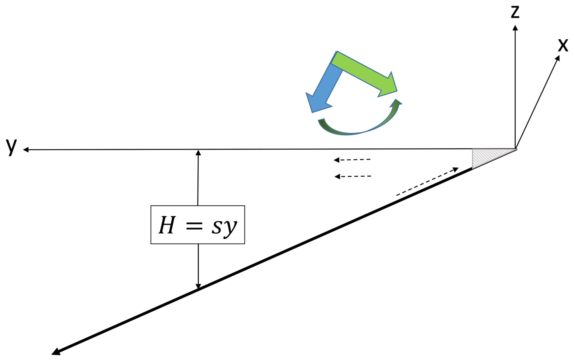
Figure 1 The linearly sloping shelf, the wind stress vectors, τ^x, shown here at angles θ=180° (blue thick arrow) and θ=270° (green thick arrow) relative to the +x direction. The angle, θ, increases in agreement with the counterclockwise rotation of the wind (curved arrow). The offshore directed surface current and the compensating onshore directed bottom current (dashed arrows) are shown in an upwelling mode, associated with a constant wind stress at θ=180°.

On a linearly sloping continental shelf, such as that sketched in Fig. 1, the layer thickness is given by H(y)=Sy so the second terms on the RHS of the $\mathrm{d}U/\mathrm{d}t$ and $\mathrm{d}V/\mathrm{d}t$ equations in system (Eq. 4) are:

$$\begin{array}{}\text{(5)}& {\displaystyle \frac{\mathit{\tau }\left(\mathrm{0}\right)-\mathit{\tau }(-Sy)}{\mathit{\rho }Sy}},\end{array}$$

where τ denotes τ^x or τ^y. The shoreline, y=0, is a special case that differs fundamentally from all y>0 points, since at y=0 both the denominator and the numerator in Eq. (5) vanish. In contrast, at y>0 the denominator is finite and the bottom stress, τ(−Sy), can be neglected compared to the wind stress, τ(0), since away from the shoreline the bottom velocity is small. In the remainder of this work, we focus on the range y>0, which eliminates the “shoreline singularity” at y=0. The immediate vicinity of the shoreline that is affected by this singularity is shaded gray in Fig. 1 and, as will be shown below, the extent of this excluded range has a negligible effect on the solution in the rest of the shelf. The gray region near the shore is the terminus of the landward directed bottom flow that balances the seaward directed surface flow that originates from the forcing by the overlying wind stress.

Although H(y) denotes the bottom slope of the shelf topography, it is used here as the depth of the Ekman layer in the bulk of the shelf, i.e., away from the gray region and above the viscous bottom layer, both of which are noted in Fig. 1. The assumption underlying this identity of bottom depth and thickness of the Ekman layer is that the viscosity dominated bottom flow occupies a layer that is thinner than H throughout the bulk of the shelf. Thus, the momentum imparted by the wind stress reaches only the top of this bottom layer, i.e., a depth approximated by H away from the gray region right next to the coast. The complex, highly viscous flow at the bottom of the shelf results in response to the direct wind-driven flow at the surface, and this bottom flow guaranties that near the coast the sea surface height remains unchanged by the surface flow. In the present work, we focus on the first-order primary dynamics of the surface wind-driven flow over a sloping bottom and ignore the second-order viscous dynamics of the bottom flow, which greatly complicates the governing equations. The combined dynamics of the surface and bottom layers is too complex to yield analytical results similar to those developed here, and we leave the inclusion of the compensating viscous bottom flow to future, primarily numerical, studies.

These considerations imply that at y>0 the dynamical system of wind driven flow on the continental shelf is given by:

$$\begin{array}{}\text{(6)}& \begin{array}{rl}& {\displaystyle \frac{\mathrm{d}x}{\mathrm{d}t}}=U,{\displaystyle \frac{\mathrm{d}y}{\mathrm{d}t}}=V,{\displaystyle \frac{\mathrm{d}U}{\mathrm{d}t}}=f_{\mathrm{0}}V+{\displaystyle \frac{{\mathit{\tau }}^x\left(\mathrm{0}\right)}{\mathit{\rho }Sy}},\\ & {\displaystyle \frac{\mathrm{d}V}{\mathrm{d}t}}=-f_{\mathrm{0}}U+{\displaystyle \frac{{\mathit{\tau }}^y\left(\mathrm{0}\right)}{\mathit{\rho }Sy}}.\end{array}\end{array}$$

In the model under study, τ^x(0) and τ^y(0) are periodic in time, while their amplitude remains constant. We therefore let τ^x(0)=Γcos (θ) and τ^y(0)=Γsin (θ) where Γ is the constant dimensional amplitude of the wind stress and θ=ωt is its direction relative to +x. Although the frequency, ω, is by definition positive, here we attach to it a sign that indicates whether the direction of the wind relative to the +x direction, θ, increases or decreases. Thus, ω>0 implies counterclockwise rotation of the wind (denoted by CCW in Orlić, 2011), while ω<0 implies clockwise rotation of the wind (denoted by CW in Orlić, 2011).

While the dimensional equations in system (Eq. 6) can be easily solved numerically, the nondimensional form minimizes the number of free parameters, which helps unravel the overall properties of the solutions (Paldor and Friedland, 2023a). Naturally, time, t, in the four-dimensional system (6), is scaled on $\frac{\mathrm{1}}{f_{\mathrm{0}}}\approx {\mathrm{10}}^{\mathrm{4}}s$. Since the analysis below is based on the smallness of the wind stress amplitude, $\mathrm{\Gamma }/\mathit{\rho }S$ cannot be used to define the length scale. Thus, we scale the velocity components U and V on the typical velocity over the shelf: U_scale=0.5 m s⁻¹. The length scale, L, of x and y is then chosen as $U_{\mathrm{scale}}/f_{\mathrm{0}}\approx \mathrm{5}$ km. The use of f₀ in the definition of L assumes, of course, that it is positive. In order for the theory to apply in the southern hemisphere, where f₀<0, one has to define the scale as $\left|f_{\mathrm{0}}\right|$, leaving in the equations a “flag” that denotes the sign of f₀. We further modify the equations by substituting $D=U-y$ for U in the nondimensional equations. As can be easily verified, D is conserved (i.e. $\mathrm{d}D/\mathrm{d}t=\mathrm{0}$) in inertial motion where the wind stress vanishes. The associated relationship between zonal velocity and meridional coordinate in inertial dynamics on a sphere or on the β-plane reflects the conservation of angular momentum (Rom-Kedar et al., 1997; Paldor and Killworth, 1988; Paldor, 2007). This study employs a perturbative method where the small parameter is the amplitude of the wind stress so it is advantageous to select a variable such as D which is time-independent when the wind stress vanishes. Following these two changes, system (Eq. 6) transforms to:

$$\begin{array}{}\text{(7)}& {\displaystyle }& {\displaystyle \frac{\mathrm{d}x}{\mathrm{d}t}}=D+y,\text{(8)}& {\displaystyle }& {\displaystyle \frac{\mathrm{d}y}{\mathrm{d}t}}=V,\text{(9)}& {\displaystyle }& {\displaystyle \frac{\mathrm{d}D}{\mathrm{d}t}}={\displaystyle \frac{\mathit{ϵ}\cos \left(\mathit{\omega }t\right)}{y}},\text{(10)}& {\displaystyle }& {\displaystyle \frac{\mathrm{d}V}{\mathrm{d}t}}=-(D+y)+{\displaystyle \frac{\mathit{ϵ}\sin \left(\mathit{\omega }t\right)}{y}},\end{array}$$

where $\mathit{ϵ}=\frac{\mathrm{\Gamma }}{\mathit{\rho }S(f_{\mathrm{0}}L{)}^{\mathrm{2}}}$ is the nondimensional amplitude of wind stress forcing and t and ω are the nondimensional time and wind stress frequency (including the sign attached to it as explained above), respectively. With the scales used here the nondimensional Coriolis frequency is equal to 1 and for the typical oceanic values of Γ=0.03 N m⁻², ρ=1027 kg m⁻³, $S={\mathrm{10}}^{-\mathrm{3}}$ and f₀L=0.5 m s⁻¹ the forcing amplitude is $\mathit{ϵ}\approx \mathrm{0.1}<\mathrm{1}$. The only free parameters of the nonlinear dynamical system (Eqs. 7–10) are the wind stress rotation frequency, ω, the wind stress amplitude, ϵ<1, and the initial values of the dependent variables. As intended, Eq. (9) ensures that $D=\mathrm{Const}.$ for ϵ=0 while U=U(t) even when the wind stresses, τ^x(0) and τ^y(0), vanish in system (Eq. 6).

A natural choice of initial velocities is that the water column is motionless at t=0 when the wind stress sets the column into motion, i.e. U(0)=0 and V(0)=0. The definition $D=U-y$ implies, therefore, that $D\left(\mathrm{0}\right)=-y\left(\mathrm{0}\right)$. Since x does not appear on the RHS of the equations in the system (Eqs. 7–10), x(0)=0 can be set without loss of generality, so the only initial condition affecting the dynamics is y(0).

A general analytical scheme that can provide insight on the solutions of the nonlinear system of equations (Eqs. 7–10) and on the trajectory of a water column on both the f-plane and the β-plane forced by a wind stress was developed recently for constant H in Paldor and Friedland (2023a). In this scheme the system is analyzed by combining Eqs. (8) and (10) to a single 2nd order equation:

$$\begin{array}{}\text{(11)}& {\displaystyle \frac{{\mathrm{d}}^{\mathrm{2}}y}{\mathrm{d}{t}^{\mathrm{2}}}}=-(D+y)+{\displaystyle \frac{\mathit{ϵ}\sin \left(\mathit{\omega }t\right)}{y}}.\end{array}$$

In the following, we will assume that the wind stress contributions in Eqs. (9) and (11) are perturbations, i.e., D≈D(0), y≈y(0) and $\mathit{ϵ}/y\left(\mathrm{0}\right)\ll y\left(\mathrm{0}\right)$. Note that the last condition can be satisfied even when ϵ is O(1), provided y(0)>3. According to Eq. (9) for $\mathit{ϵ}/y\left(\mathrm{0}\right)\ll \mathrm{1}$, D varies slowly with time, which implies that the dynamics of the (V, y) subsystem is that of a quasi-particle in a slowly varying potential. The following analysis focuses on the (V, y, D) subsystem, Eqs. (9) and (11) for slowly varying D.

2.2 The linear solutions

The initial conditions detailed above imply that inertial oscillations (i.e. in the absence of body forces) are filtered out from the dynamics since for ϵ=0 a water column remains in its initial location at all t when V(0)=0 and $D\left(\mathrm{0}\right)=-y\left(\mathrm{0}\right)$. The first step of the analysis is to linearize y(t) and D(t) about their respective initial values y(0) and −y(0), that is, to substitute: $y\left(t\right)=y\left(\mathrm{0}\right)+\mathit{\delta }y\left(t\right)$ and $D\left(t\right)=-y\left(\mathrm{0}\right)+\mathit{\delta }D\left(t\right)$ in Eqs. (9) and (11) where δy(t) and δD(t) are $O(\mathit{ϵ}/y(\mathrm{0}\left)\right)$. The resulting linear system is:

$$\begin{array}{}\text{(12)}& {\displaystyle }& {\displaystyle \frac{{\mathrm{d}}^{\mathrm{2}}\mathit{\delta }y}{\mathrm{d}{t}^{\mathrm{2}}}}=-(\mathit{\delta }D+\mathit{\delta }y)+{\displaystyle \frac{\mathit{ϵ}\sin \left(\mathit{\omega }t\right)}{y\left(\mathrm{0}\right)}},\text{(13)}& {\displaystyle }& {\displaystyle \frac{\mathrm{d}\mathit{\delta }D}{\mathrm{d}t}}={\displaystyle \frac{\mathit{ϵ}\cos \left(\mathit{\omega }t\right)}{y\left(\mathrm{0}\right)}}.\end{array}$$

The initial conditions associated with this 3rd order differential system are: $\mathit{\delta }D\left(\mathrm{0}\right)=\mathrm{0}=\mathit{\delta }y\left(\mathrm{0}\right)=\frac{\mathrm{d}\mathit{\delta }y\left(\mathrm{0}\right)}{\mathrm{d}t}$. The 3 initial conditions define a unique solution of the differential problem. A direct integration of Eq. (13) yields:

$$\begin{array}{}\text{(14)}& \mathit{\delta }D={\displaystyle \frac{\mathit{ϵ}}{\mathit{\omega }y\left(\mathrm{0}\right)}}\sin \left(\mathit{\omega }t\right),\end{array}$$

which satisfies the initial condition δD(0)=0. For the solution of Eq. (12) we assume a form that includes the function G(t) that solves the inhomogeneous part of this equation, i.e.:

$$\begin{array}{}\text{(15)}& \mathit{\delta }y=a\sin \left(\mathit{\omega }t\right)+G\left(t\right).\end{array}$$

The constant a and the function G(t) need to be determined by the initial conditions. Substituting this form of solution in Eq. (12) yields:

$$\begin{array}{}\text{(16)}& \begin{array}{rl}{\displaystyle \frac{{\mathrm{d}}^{\mathrm{2}}G}{\mathrm{d}{t}^{\mathrm{2}}}}& -{\mathit{\omega }}^{\mathrm{2}}a\sin \left(\mathit{\omega }t\right)=-\left({\displaystyle \frac{\mathit{ϵ}}{\mathit{\omega }y\left(\mathrm{0}\right)}}\sin \left(\mathit{\omega }t\right)+a\sin \left(\mathit{\omega }t\right)+G\right)\\ & +{\displaystyle \frac{\mathit{ϵ}\sin \left(\mathit{\omega }t\right)}{y\left(\mathrm{0}\right)}}.\end{array}\end{array}$$

The sin (ωt) terms in Eq. (16) yield:

$$\begin{array}{}\text{(17)}& -{\mathit{\omega }}^{\mathrm{2}}a=-\left({\displaystyle \frac{\mathit{ϵ}}{\mathit{\omega }y\left(\mathrm{0}\right)}}+a\right)+{\displaystyle \frac{\mathit{ϵ}}{y\left(\mathrm{0}\right)}}\end{array}$$

while the remaining terms yield: $\frac{{\mathrm{d}}^{\mathrm{2}}G}{\mathrm{d}{t}^{\mathrm{2}}}=-G$ i.e. oscillations at the inertial frequency, ±1, that appear due to the presence of the wind forcing in the O(ϵ) terms. The initial conditions imposed on G are: G(0)=0 and $\mathrm{d}G\left(\mathrm{0}\right)/\mathrm{d}t=-a\mathit{\omega }$ to ensure that δy(0)=0 and $\mathrm{d}\left(\mathit{\delta }y\right(\mathrm{0}\left)\right)/\mathrm{d}t=\mathrm{0}$. The resulting solution of G(t) that satisfies these initial conditions is: $G\left(t\right)=-\mathit{\omega }a\sin \left(t\right)$, which implies that

$$\begin{array}{}\text{(18)}& \mathit{\delta }y\left(t\right)=a\sin \left(\mathit{\omega }t\right)-a\mathit{\omega }\sin \left(t\right).\end{array}$$

Finally, Eq. (17) yields the expression for a:

$$\begin{array}{}\text{(19)}& a=-{\displaystyle \frac{\mathit{ϵ}}{\mathit{\omega }y\left(\mathrm{0}\right)(\mathrm{1}+\mathit{\omega })}}.\end{array}$$

Substituting the expressions of a and G(t) derived above in the general expressions of y(t) and combining it with the solution for D(t) yields:

$$\begin{array}{}\text{(20)}& {\displaystyle }\begin{array}{rl}y\left(t\right)=& y\left(\mathrm{0}\right)+\mathit{\delta }y\\ & =y\left(\mathrm{0}\right)-{\displaystyle \frac{\mathit{ϵ}}{\mathit{\omega }y\left(\mathrm{0}\right)(\mathrm{1}+\mathit{\omega })}}\left[\sin \right(\mathit{\omega }t)-\mathit{\omega }\sin t],\end{array}\text{(21)}& {\displaystyle }D\left(t\right)=D\left(\mathrm{0}\right)+\mathit{\delta }D=-y\left(\mathrm{0}\right)+{\displaystyle \frac{\mathit{ϵ}}{\mathit{\omega }y\left(\mathrm{0}\right)}}\sin \left(\mathit{\omega }t\right).\end{array}$$

The solution for y(t) has a strong resonance effect near $\mathit{\omega }=-\mathrm{1}$. As can be expected, the time-dependent solution of the problem has two fundamental frequencies: The inertial frequency, −1, (that is, −f₀ in dimensional units) and ω, the frequency of the wind forcing. The corresponding solutions for x(t) can be derived by inserting Eqs. (20) and (21) in Eq. (7).

Having completed the analysis of the $O(\mathit{ϵ}/y(\mathrm{0}\left)\right)$ terms in Eqs. (9) and (11) we turn now to the analysis of the $O({\mathit{ϵ}}^{\mathrm{2}}/y(\mathrm{0}{)}^{\mathrm{2}})$ terms, which can be better compared with the solutions obtained by numerical simulations.

2.3 Second order effects in the wind stress and the drift in x

The constant drift in x appears if $D+y=\mathit{\delta }D+\mathit{\delta }y$ in Eq. (7) has a constant component. Time averages of the linear (in ϵ) components of δD and δy in Eqs. (20) and (21) do not produce such constant components since all terms are purely oscillatory. We, therefore, include $O\left(\right(\mathit{ϵ}/y\left(\mathrm{0}\right){)}^{\mathrm{2}})$ terms in Eqs. (9) and (11) to get:

$$\begin{array}{}\text{(22)}& {\displaystyle \frac{\mathrm{d}\mathit{\delta }D}{\mathrm{d}t}}={\displaystyle \frac{\mathit{ϵ}\cos \left(\mathit{\omega }t\right)}{y\left(\mathrm{0}\right)}}-{\displaystyle \frac{\mathit{ϵ}\cos \left(\mathit{\omega }t\right)}{y(\mathrm{0}{)}^{\mathrm{2}}}}\mathit{\delta }y,\end{array}$$

and

$$\begin{array}{}\text{(23)}& {\displaystyle \frac{{\mathrm{d}}^{\mathrm{2}}\mathit{\delta }y}{\mathrm{d}{t}^{\mathrm{2}}}}=-(\mathit{\delta }D+\mathit{\delta }y)+{\displaystyle \frac{\mathit{ϵ}\sin \left(\mathit{\omega }t\right)}{y\left(\mathrm{0}\right)}}-{\displaystyle \frac{\mathit{ϵ}\sin \left(\mathit{\omega }t\right)}{y(\mathrm{0}{)}^{\mathrm{2}}}}\mathit{\delta }y,\end{array}$$

where for δy we use the oscillatory linear solution (Eq. 18). Note that the RHS of Eq. (22) has zero average components only. Therefore, the solution of δD also has only zero average components. In contrast, the RHS of Eq. (23) has oscillating zero average components, but also a nonzero averaged term: $\mathit{ϵ}\frac{\sin \left(\mathit{\omega }t\right)}{y(\mathrm{0}{)}^{\mathrm{2}}}\mathit{\delta }y$. Thus, the solution of Eq. (23) has a constant component that originates from the sin (ωt) term in δy via: $〈\mathit{ϵ}\frac{\sin \left(\mathit{\omega }t\right)}{y(\mathrm{0}{)}^{\mathrm{2}}}\mathit{\delta }y〉=\frac{{\mathit{ϵ}}^{\mathrm{2}}}{\mathrm{2}\mathit{\omega }y\left(\mathrm{0}{)}^{\mathrm{3}}\right(\mathrm{1}+\mathit{\omega })}$. The zonal drift associated with this term is:

$$\begin{array}{}\text{(24)}& U_{\mathrm{d}}=〈{\displaystyle \frac{\mathrm{d}x}{\mathrm{d}t}}〉=\langle \mathit{\delta }y\rangle ={\displaystyle \frac{{\mathit{ϵ}}^{\mathrm{2}}}{\mathrm{2}y\left(\mathrm{0}{)}^{\mathrm{3}}\mathit{\omega }\right(\mathrm{1}+\mathit{\omega })}}.\end{array}$$

This drift is much stronger (resonant) near $\mathit{\omega }=-\mathrm{1}$ and changes sign at this frequency in accordance with the resonance in δy at this value. The existence of this constant, 2nd order, longshore drift is quite surprising in view of the periodically rotating wind stress forcing and the traditional (steady) 90° angle between the wind stress and the surface transport. The direction of the drift is positive except for $-\mathrm{1}<\mathit{\omega }<\mathrm{0}$ in which case ω(1+ω) in the denominator is negative. In an entirely different Eulerian model in which the “shelf” is merely a transition zone between a finite-depth open ocean and a shallower, uniform-depth coastal region, Loder (1980) proposed a heuristic explanation for the long-shelf drift in terms of the Eulerian long-shore velocity gradient on both sides of the “shelf”. Although this explanation does not apply to the purely Lagrangian model studied here, the emergence of a long-shore drift over a sloping bottom seems to be of general applicability, but the dependence of the drift's direction on the forcing frequency probably characterizes only the present model.

Numerical solutions of system (Eq. 7–10) that verify the validity of the analytic approximations developed here are presented in Sect. 3.

3 Numerical confirmations

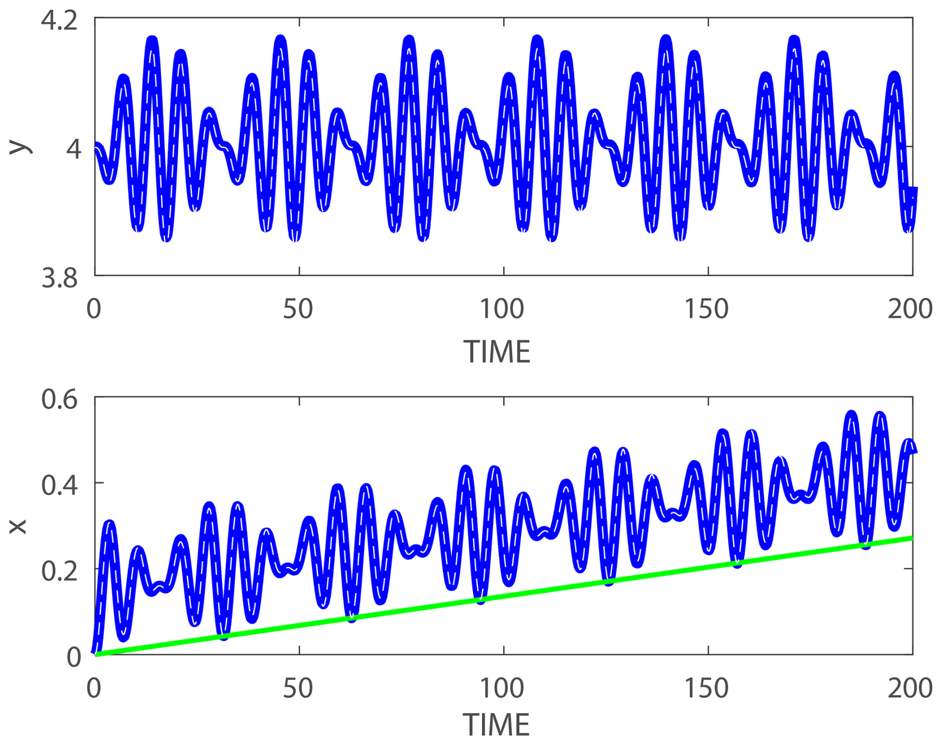
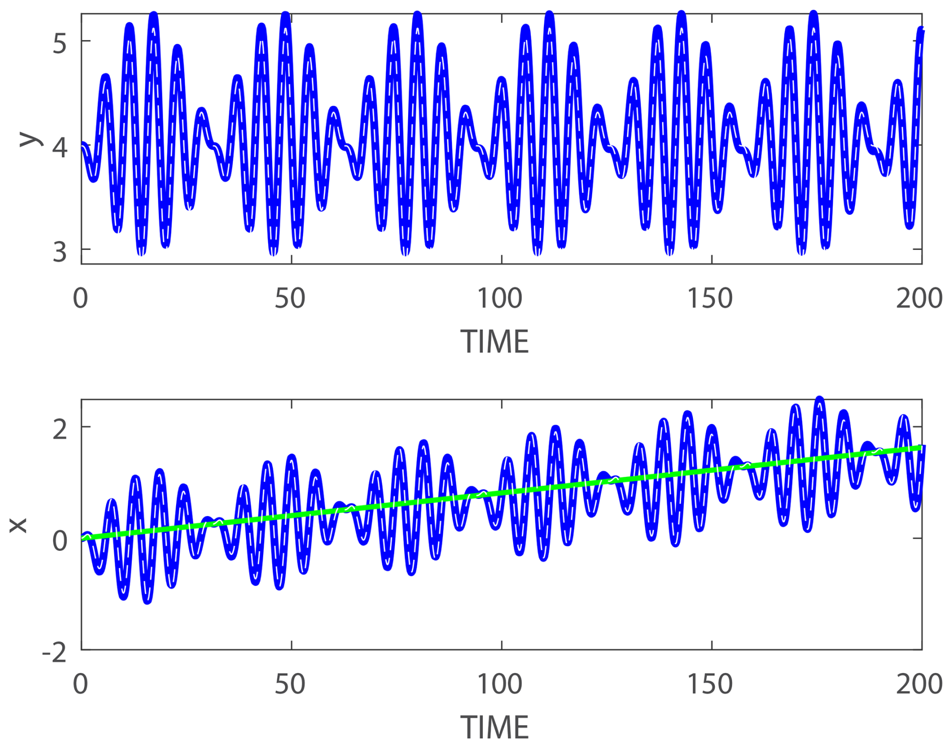
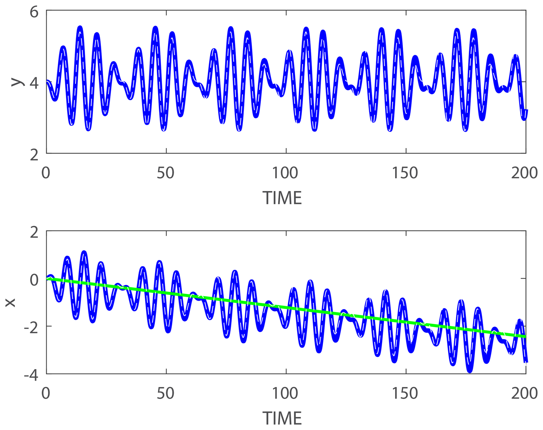
Four examples comparing the theory (white dashed curves) and simulations (blue curves) near $\mathit{\omega }=+\mathrm{1}$ and $\mathit{\omega }=-\mathrm{1}$ i.e. $\mathit{\omega }=\pm \mathrm{0.8}$ and $\mathit{\omega }=\pm \mathrm{1.2}$ are shown in Figs. 2–5. The initial conditions used in all simulations are x(0)=0, V(0)=0, $D\left(\mathrm{0}\right)=-y\left(\mathrm{0}\right)$ and y(0)=4. The simulations were carried out using MATLAB routine ODE45, which is based on Runge–Kutta formula (4, 5), with relative and absolute tolerances of 10⁻⁹. The figures show the accuracy of the approximate analytic expressions (blue thick solid curves) compared to the simulated solutions (white thin dashed curves) even when ϵ=0.5 is not very small (recall that for realistic oceanic values ϵ<1 and that the small parameter is $\mathit{ϵ}/y\left(\mathrm{0}\right)$). For smaller values of ϵ the approximate analytic expressions are even closer to the numerical solutions. The x(t) plots (lower panels) also demonstrate the validity of the approximate longshore drift given by Eq. (24) shown by the green straight lines in these panels. As anticipated analytically, the longshore drift is directed in the −x direction when $-\mathrm{1}<\mathit{\omega }<\mathrm{0}$ and in the +x direction when $\mathit{\omega }<-\mathrm{1}$ and ω>0. Regarding the other variables of the dynamics, in addition to the direction of longshore drift, the only other appreciable difference between positive and negative forcing frequencies is in the δD(t) curves (results not shown).

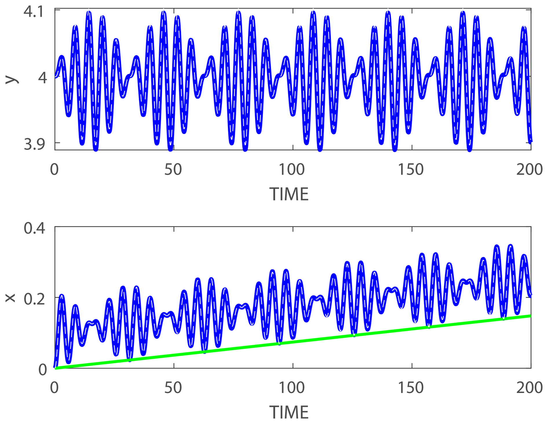
Figure 2 A comparison between direct simulations (dashed white curves) and the explicit expressions developed in Sect. 2 for small ϵ (solid thick blue curves) of: y (upper panel) and x (lower panel) for ω=1.2 and ϵ=0.5. The green straight line in the lower panel shows the approximate expression for the drift given in Eq. (24).

Figure 3 Same as Fig. 2 but for ω=0.8.

Figure 4 Same as Fig. 2 but for $\mathit{\omega }=-\mathrm{1.2}$.

Figure 5 Same as Fig. 2 but for $\mathit{\omega }=-\mathrm{0.8}$.

4 Summary and discussion

In this work, we developed a theory of surface transport on a linearly sloping continental shelf forced by periodically rotating wind stress. The perturbative analysis is based on the smallness of the nondimensional amplitude of the rotating wind forcing. The shoreline singularity where the shelf's mean depth, H, vanishes does not appreciably affect the solution far from the shoreline, since the solution there is independent of the seaward extent of the region containing the singular point. Analysis and numerical simulations show that although the wind forcing is rotary and periodic, there exists a longshore drift directed in the −x direction when $-\mathrm{1}<\mathit{\omega }<\mathrm{0}$ and in the +x direction for values of ω outside this range.

The resonance expected to dominate the dynamics at $\mathit{\omega }=-\mathrm{1}$, that is, for a CW rotation at the local inertial frequency is evident in the drift in x. which is about 4 times larger near $\mathit{\omega }=-\mathrm{1}$ (lower panels in Figs. 4 and 5) than near $\mathit{\omega }=+\mathrm{1}$ (lower panels in Figs. 2 and 3). The ratio between the drift in x for ω near −1 and ω near +1 increases drastically when the frequency approaches these values. For ϵ=0.1 (to ensure that the perturbation analysis is valid), the ratio between the drifts in x for $\mathit{\omega }=-\mathrm{0.95}$ and $\mathit{\omega }=+\mathrm{0.95}$ is O(50) (results not shown). The resonance at $\mathit{\omega }=-\mathrm{1}$ originates from the general solution of the homogeneous equation (mentioned only briefly in the above analysis, which focuses on the particular solution of the inhomogeneous equation) that describes inertial oscillations that rotate clockwise at the local Coriolis frequency, f₀, denoted as −1 in the notation used here.

As discussed in the Introduction, in the case of a uniform H periodic rotary wind forcing yields a range of ω in which the surface transport is directed left of the wind stress. To show that this counterintuitive result exists also on the shelf one has to compare $U+iV=\mathrm{d}x/\mathrm{d}t+i\mathrm{d}y/\mathrm{d}t$ to ${\mathit{\tau }}^x+i{\mathit{\tau }}^y=\cos \left(\mathit{\omega }t\right)+i\sin \left(\mathit{\omega }t\right)$ in the particular solution (i.e. after eliminating inertial oscillations from the solution of U+iV). Substituting Eq. (20) (without the sin t term) and Eq. (21) in Eq. (7) and adding to the resulting equation i times the derivative of Eq. (20) yields:

$$\begin{array}{}\text{(25)}& U+iV={\displaystyle \frac{\mathit{ϵ}}{y\left(\mathrm{0}\right)}}\left({\displaystyle \frac{-i}{\mathrm{1}+\mathit{\omega }}}\right)\left({\mathit{\tau }}^x+i{\mathit{\tau }}^y\right).\end{array}$$

The surface transport on the LHS of this expression is directed to the left of the wind stress for $\mathit{\omega }<-\mathrm{1}$. This result extends the result originally derived by Orlić (2011) in a basin of uniform H to the continental shelf. As noted above, the CW notation used in Orlić (2011) where only positive ω values were allowed, is represented in the present study by negative ω values (and CCW by positive ω values).

This last result is of primary observational importance as it predicts that along a coast dominated by the daily transition from sea breeze during daytime to land breeze during nighttime the direction of the longshore drift is determined by the sense of wind rotation (CW or CCW i.e. ω<0 or ω>0) and by the latitude (that determines the Coriolis frequency). The theory developed here should be applied to observations of the trajectories of drogued surface drifters on the shelf under known wind conditions. Our results should also be compared to simulations by Ocean General Circulation Models (OGCM). However, the reader is reminded that our model deals with the vertically averaged velocity, so care should be exercised when comparing our results to OGCM simulations where a surface boundary layer and an inviscid interior exist.

From a theoretical perspective, mass conservation should be applied to the solutions found here to assess whether or not periodic rotating wind stresses induce upwelling or downwelling. In the Lagrangian formulation used here, x(t) and y(t) are dependent variables that quantify the temporal changes in the coordinates of a particular water column. Thus, $\mathrm{d}U/\mathrm{d}x$ and $\mathrm{d}V/\mathrm{d}y$ do not have the Eulerian meaning of components of horizontal divergence and only imply the co-variation of pairs of dependent variables. In the Lagrangian framework, where the only independent variable is time, conservation of mass in an incompressible fluid is determined by the Jacobian of the coordinate transformation between 0 and t: $h\left(\mathrm{0}\right)=h\left(t\right)J\left(x\right(t),y(t);x(\mathrm{0}),y(\mathrm{0}\left)\right)$ where h is the height of the water column and $J\left(x\right(t),y(t);x(\mathrm{0}),y(\mathrm{0}\left)\right)=\left(\frac{\mathrm{d}x\left(t\right)}{\mathrm{d}x\left(\mathrm{0}\right)}\frac{\mathrm{d}y\left(t\right)}{\mathrm{d}y\left(\mathrm{0}\right)}-\frac{\mathrm{d}x\left(t\right)}{\mathrm{d}y\left(\mathrm{0}\right)}\frac{\mathrm{d}y\left(t\right)}{\mathrm{d}x\left(\mathrm{0}\right)}\right)$ is the Jacobian of the coordinate transformation from (x(0), y(0)) to (x(t), y(t)) (Bennett, 2006; Milne-Thomson, 1996; Paldor, 2025). In Eq. (24) x(0) is an integration constant, so $\frac{\mathrm{d}x\left(t\right)}{\mathrm{d}x\left(\mathrm{0}\right)}=\mathrm{1}$ while y(t) is independent of x(0) so $\frac{\mathrm{d}y\left(t\right)}{\mathrm{d}x\left(\mathrm{0}\right)}=\mathrm{0}$ i.e. $\frac{h\left(\mathrm{0}\right)}{h\left(t\right)}=\frac{\mathrm{d}y\left(t\right)}{\mathrm{d}y\left(\mathrm{0}\right)}$. In Eq. (20) y(0) appears in the expression of y(t)−y(0) so $\frac{\mathrm{d}y\left(t\right)}{\mathrm{d}y\left(\mathrm{0}\right)}\ne \mathrm{1}$ and, depending sensitively on the value of ω, $\frac{h\left(\mathrm{0}\right)}{h\left(t\right)}$ can be greater than 1 or less than 1 i.e., periodic stress can generate mean upwelling or downwelling. An examination of these results regarding the dependence of convergence or divergence on the forcing frequency should be examined using an OGCM along with the results associated with the direction of long-term longshore drift by the rotary wind forcing. The two extensions, as well as the identity assumed here between bottom depth and thickness of the surface Ekman layer in the bulk of the shelf, should be confirmed in future studies based on OGCM simulations.