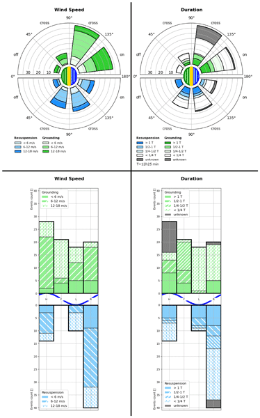
Groundings of drifters in the Wadden Sea inform the transport of floating macroplastic

We study floating marine macro plastic pollution with a dedicated campaign where we released and tracked 24 shallow surface drifters in the Dutch Wadden Sea, an intertidal region where water dynamics are driven by semi-diurnal tides and wind. The campaign captured water surface transport patterns, and around 150 observations of the drifters interacting with the coast and mudflats, where groundings of varying durations occurred. We identify these transitions in the recorded trajectories from manual inspection, and formulate and evaluate a statistical approach for the automatic detection of grounded drifters. We then characterize the transitions by relating them to the coinciding wind conditions and tides, and with the duration of the groundings. The results of this analysis generally agree with the intuitions that wind towards the coast increases the frequency of interactions and that the drifters are rarely re-floated during falling tides. Furthermore, we find that groundings tend to be shorter duration when they occur shorter before the next high tide. We present multiple visualizations that characterize the groundings in more detail. The results provide a statistical characterization of coastal interactions that can be integrated in models and used for the planning of beach-cleanups. They may be improved by considering the specific environmental conditions of the campaign, and by analyzing the influence of the weight and size of the drifters, which are both larger than typical floating macroplastic.

1 Introduction

The Wadden Sea is a shallow body of water bordering the north coast of the Netherlands and west coast of Germany and Denmark, with numerous channels situated between the Frisian Islands that connect it to the North Sea. It holds unique ecosystems and geological features, which is why it has been listed as an UNESCO world heritage site in 2009 (Common-Wadden-Sea-Secretariat, 2026; Colina Alonso et al., 2021; Kraan et al., 2010). As a water system, it consists of coastal wetlands and tidal basins that border the shelf sea across a range of barrier islands and that have multiple inflows from rivers. Its dynamics result from interactions between the semidiurnal tides of the region and residual currents of the North Sea, from wind stress that generates waves and surface currents, from freshwater inputs by river runoffs, and from the bathymetry and shape of the coast (Deyle et al., 2024; Fajardo-Urbina et al., 2023; Ricker et al., 2021; Meyerjürgens et al., 2019; Maas, 1997; Gräwe et al., 2016).

The prevailing stresses on marine ecosystems through climate change, marine pollution and other unsustainable interventions are concerns for the Wadden Sea (Eriksson et al., 2010; Kabat et al., 2012). A major contributor to the pollution is plastic debris (Neumann et al., 2014), where areas close to mainland are accumulating regions for floating macroplastic, i.e., buoyant pieces of plastic larger than 5cm (Kaandorp et al., 2023). Marine plastic enters the seas as discharge from rivers, mismanaged waste from ships or fisheries, and littering at the coast (Schöneich-Argent and Freund, 2020; González-Fernández et al., 2021). The increase in use of plastic items over the last decades coincides with a growing contamination of open waters. This poses an environmental threat, both as an obstacle for marine life, as well as by the risks arising from an increase in microscopic pollution after the fragmentation of plastic waste into micro- and nano-plastics (Dris et al., 2020). Litter at beaches also harms the touristic value of regions at the coast. Understanding the transport of floating macroplastic thus contributes to the study and mitigation of these issues.

Hydrodynamic and atmospheric models can be used in Lagrangian particle tracking simulations to model the dispersion of plastic pieces in open waters (Ricker et al., 2021; Critchell et al., 2015; Mørk et al., 2026). Multiple numerical studies have been conducted for the Wadden Sea to examine the transport of water masses, its variability with respect to wind patterns and seasonality, and dispersion (Fajardo-Urbina et al., 2023; Donatelli et al., 2022; Duran-Matute et al., 2014). These make use of estuarine models (Burchard and Bolding, 2002) and particle tracking (Delandmeter and van Sebille, 2019; Lange and van Sebille, 2017). Accurately representing marine plastic transport in coastal areas also requires a model for littoral-coast transitions, which further increases the complexity of such studies. The reliability of both the simulation outcomes and of the hydrodynamic models can be improved with in-site measurements from stations at the coast or in the water (Meyerjürgens et al., 2019; Morey et al., 2018).

Here, we report on a measurement campaign from November 2023 of 24 floating drifters at the western Wadden Sea. This experimental Lagrangian sampling is the first measurement of its kind in the Dutch Wadden Sea and also provides an additional dataset to the sparsely sampled North Sea area (Deyle et al., 2024; Meyerjürgens et al., 2019; Fajardo-Urbina et al., 2023; Medina-Rubio et al., 2026; Elias et al., 2022). A particular process that is captured in the dataset is the occurrence of grounding events where drifters temporarily settle down on tidal flats. The focus of the data analysis here lies on these events and groundings at the coast, which are an important component to better understand the displacement of marine debris, and to predict accumulation regions of stranded plastic on the coast (Critchell and Lambrechts, 2016; Meyerjürgens et al., 2019; Pawlowicz, 2021). These forecasts in turn are valuable to beach cleanup efforts, which are mainly organized as volunteering activities. Knowledge about general hot spots and specific grounding patterns can inform decisions on when and where beach cleanups are most effective. Another motivation to study grounding of macroplastic is that the transitions between water and land take part in the mechanical decomposition of the plastic (Takeda and Isobe, 2024; Kaandorp et al., 2021).

We describe two systematic approaches to manually and to statistically identify grounding events in trajectories, and apply them to the campaign observations. By comparing the two outcomes, we verify the reliability of the grounded statistic and its parameterization. We then classify the groundings with respect to environmental conditions – wind and tidal state – and the grounding duration.

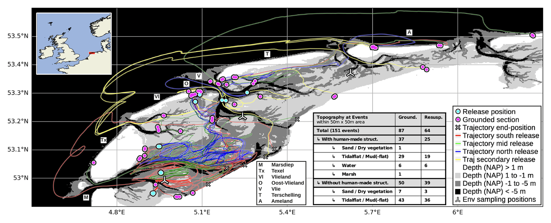
Figure 1 Trajectories (lines) and release/grounding locations (circles) of the campaign (van Sebille, 2024) drawn over a bathymetry map. The table at the bottom center lists the number of events categorized by the topography within an area of 50 m × 50 m. This illustration synchronizes with Fig. 4 by matching the colors of the trajectories with the markings at the beginning of the release timeline, and by locating the three positions where environmental conditions (wind, water level) were sampled for reference. More detailed versions of this figure are contained in Appendix A, and a simplified vector graphics rendering of this figure is provided in Fig. S1 in the Supplement. Maps and bathymetry generated with (Map data ©Crown Copyright, Met Office, 2010–2015, licensed under OGL v3.0; Additional layers ©Waddenregister, 2026 (CC-BY 4.0)).

2 Methods

2.1 Campaign

We released 24 drifters on 14 November 2023, as summarized in Fig. 1. This took place in three locations near the Dutch island Texel, approximately 9 km apart, and before and during the low tide at 13:30 UTC. One batch of six drifters was re-deployed in a secondary release at multiple locations east of the Dutch island Vlieland on 20 November. For the selection of the initial release locations and times, we considered the typical sea surface dynamics and local bathymetry, and consulted personnel at the Royal Netherlands Institute for Sea Research (NIOZ). We also estimated the trajectories with numerical simulations and weather forecasts, in particular the tidal cycles on the release day. The intention was for the drifters to be moved out of the Wadden Sea and into the North Sea during a few tidal cycles. We released the drifters as nested triplets in a triangular pattern at two of the three locations, and as two triplets at the third location. From this, trajectories of each triplet can be analyzed as three different pair releases or one triplet release. The release-pattern is self-similar, with the smaller scale of 10 m for the nested triplets, and the larger scale of 100 m for combinations of triplets. The releases on the smaller scales are only an approximation of a triangular pattern, and the initial drift after the deployment was sometimes influenced by ship maneuvers.

Stokes Drifters were used to collect the measurements. They are shallow and disk-shaped trackers produced by MetOcean (MetOcean, 2026). They have a diameter of 24 cm, a height of 4 cm and a weight of 1 kg. These drifters lie flat in the water, their profile reaches roughly 1.5 cm out of the water surface. This makes them sensitive to dynamics in the uppermost centimeters of the water column and to air-drag (Medina-Rubio et al., 2026; Morey et al., 2018). For tracking, the drifters contain a positioning system (GNSS), and for communication, they carry a transmitter for the Iridium satellite system. Furthermore, the Stokes Drifters record the sea surface temperature (SST) and the orientation of the drifter in the water. Power is provided by a set of 10 AA-alkaline batteries. The operational time depends on the sampling configuration, consisting of a sampling interval and an upload interval. The sampling interval determines the time between measurements. We set it to 5 min (resulting in time-series with approximately 5.2 min intervals) to record with the highest available temporal resolution. The upload interval regulates after how many measurements the collected data are transmitted. Since these transmissions are power intense, we set this value to 12, which resulted in one transmission attempt per hour.

2.1.1 Citizen Involvement

The campaign involved citizen contributions both for the funding and the observation and recovery of the drifters. Before the campaign, the University Fund of Utrecht University organized a crowdfunding campaign for the project. During the campaign, citizens were involved because the drifters are spotted once washed ashore. Anticipating this, we designed the sticker shown in Appendix F to convey a brief message to finders. The intention was that finders send an email with a picture of the drifter for documentation, without moving the drifter to another location. In this manner, grounding and resuspension processes of the drifters should remain part of the observations. In addition, once a reported drifter had reached the end of its measurement period, we asked the finders to return the drifter via post. We received 35 sightings, and recovered 12 of the 24 released drifters.

2.1.2 Data Collection and Processing

We collected the transmitted measurements and manually removed any sections at the end of the recordings that originated from the transport of the drifters by people on land. Some drifters have also been redeployed after a first collection, which we record as independent deployments. The analysis that follows is based on the drifter trajectories of this dataset (van Sebille, 2024).

The raw trajectories are processed to derive a set of homogeneous time-series. In a first step, we remove outliers that appear as abrupt changes of location. It was found that filtering out displacements between consecutive measurements of more than 50 km in either the longitudinal or latitudinal direction provides satisfactory results. In the second step, we regularized the time-steps of the trajectories by splitting up the trajectories at time-steps larger than a chosen threshold t_max, and by averaging the timestamps and positions of consecutive measurements with time-steps smaller than a chosen threshold t_min. This step resulted in a few trajectories with only a small number of positions. We removed these in a third step by requiring a minimum total duration T_min and a minimum number of samples N_min of a time-series. The parameter choice for the analysis here are 20 min for t_max, 2.5 min for t_min, 1.5 h for T_min, and 12 for N_min.

We recreate the water levels, the topological surroundings, and the wind conditions encountered by the drifters from a MATROOS dataset (Rijkswaterstaat, 2026), a high-resolution regional bathymetry map (Waddenregister, 2026), OpenStreetMap (OpenStreetMap, 2017), and the ERA5 reanalysis (ERA5, 2026).

Table 1 Terminology to describe the transition events of drifters or floating macroplastic.

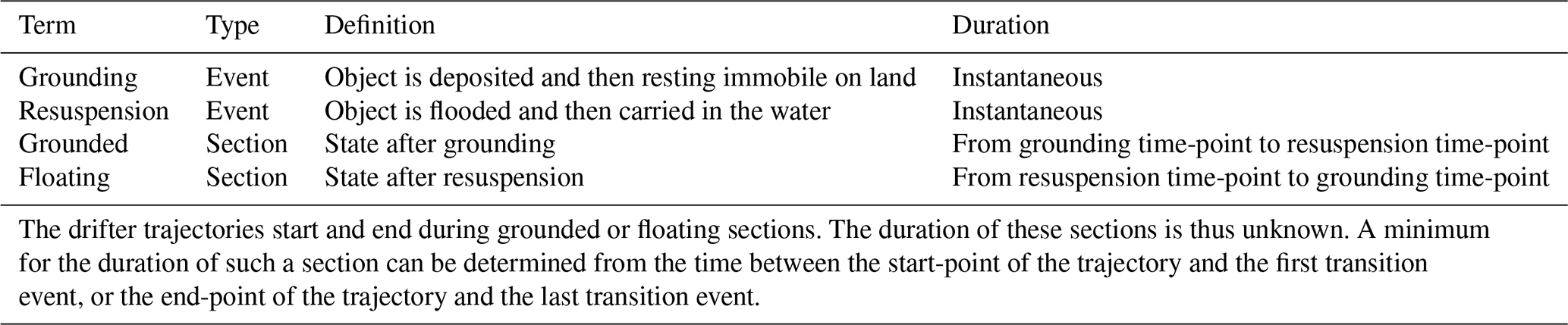
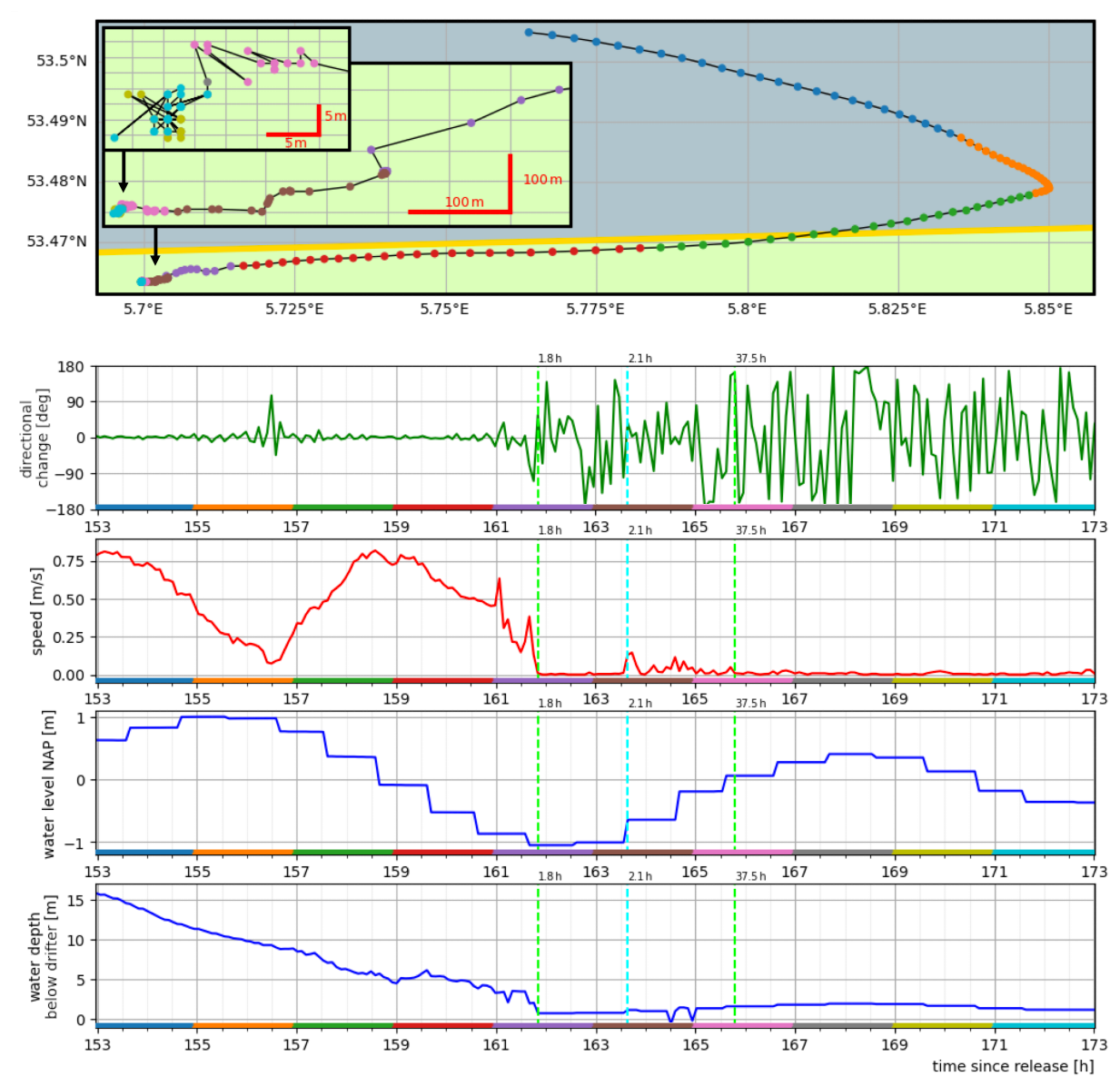
Figure 2 Typical observations of a drifter during floating and grounded sections: From top to bottom, the plots show the trajectory and two breakouts with a zoom-in on the last 11 and 7 h, the change in direction between consecutive measurements (green), the speed (red), the water level at the drifters position and time (upper blue), and the water depth below the drifter (lower blue) are shown. The color-sequence along the time axis of the line-plots is matched with the way-points of the trajectory. The vertical green and blue lines mark grounding and resuspension events, respectively, and the times above these lines indicate the duration of the sections. Steps in the water level time series result from two subsequent positions of the trajectory being closest to two different grid cells of the water level dataset (Rijkswaterstaat, 2026). The sampling frequency is 5.2 min. Maps and bathymetry generated with (Map data ©Crown Copyright, Met Office, 2010–2015, licensed under OGL v3.0; Water depth based on ©Waddenregister, 2026 (CC-BY 4.0)).

2.2 Identifying Grounded and Floating Sections and Transition Events

The transport of floating macroplastic in coastal regions can be described with the terminology summarized in Table 1, as a sequence of grounding and resuspension events that border grounded and floating sections. Figure 2 shows a drifter-trajectory from the campaign with multiple floating and grounded sections. The characteristic star-shaped pattern is formed by inaccuracies of the GNSS receivers when the position of the drifter remains constant for multiple measurements. This contrasts with the otherwise directional and smoother features in parts of the trajectory when the drifter is afloat. The grounding and resuspension events occur at the transitions between these two regimes.

2.2.1 Manual Grounding Identification

We visually inspected and annotated the trajectories with labels for grounding and resuspension events, based on the guideline described in Appendix D. Each trajectory time-step is then annotated as (manual) grounded or (manual) floating. For validation, ten trajectories were annotated by two coders. Comparing the two outcomes per time-step gives an agreement of 94 % for one trajectory, and above 97 % for the other nine ones. A comparison per event shows that roughly 75 % of the labels have a correspondence within five time-steps (30 min), 10 % agree within up to 19 time-steps (2 h), and 15 % of the annotations do not have a correspondence. The mismatches from the last category are annotations of four shorter grounded sections, where the grounding and resuspension events are 30–60 min apart.

2.2.2 Statistical Indication of Grounded Sections

The plots in Fig. 2 show that quantities derived from the trajectories display characteristic behaviors in correlation with grounded sections. We subsequently formalize this observation to design a statistic that indicates a grounded drifter, which should be applicable for different GNSS systems and sampling strategies. The GNSS trajectories can be written as time series of positions $p\left(t\right)=\left(\text{lon}\right(t),\text{lat}(t\left)\right)$ at sampling times $t=t_{\mathrm{1}},t_{\mathrm{2}},\mathrm{\dots },t_N$. We measure distances between recorded positions with the geodetic distance $d_{\mathrm{g}}(p_{\mathrm{1}},p_{\mathrm{2}}):=|p_{\mathrm{2}}-p_{\mathrm{1}}|$ and locally define angles between displacements $\mathrm{\measuredangle }(p_{\mathrm{2}}-p_{\mathrm{1}},p_{\mathrm{3}}-p_{\mathrm{1}})\in [-\mathrm{180}\mathit{°},\mathrm{180}\mathit{°}]$ from a projection of the positions to rectangular coordinates.

2.2.3 Definition of the Grounded Statistic

The speed v(t) as a discrete time derivative of the position

$$v\left(t_{\mathrm{i}}\right):={\displaystyle \frac{\left|p\right(t_{i+\mathrm{1}})-p(t_{\mathrm{i}}\left)\right|}{t_{i+\mathrm{1}}-t_{\mathrm{i}}}}$$

is low when the drifter is immobile. This occurs when a drifter is suspended on land, but it can also be the result of specific states of the water surface, for example at the turning points of tidal cycles. A related quantity is the displacement D(t,ΔT) during a chosen time interval ΔT

$$D(t,\mathrm{\Delta }T):=\left|p\right(t+\mathrm{\Delta }T/\mathrm{2})-p(t-\mathrm{\Delta }T/\mathrm{2}\left)\right|$$

where the continuous time $t\pm \mathrm{\Delta }T/\mathrm{2}$ can be matched to the discrete recorded times t_i by an interpolation scheme. We choose to use nearest neighbor interpolation p(t)→p(t_i), $i=\text{argmin}\mathit{\left\{}\right|t_{\mathrm{i}}-t\left|\mathit{\right\}}$. The distance D(t,ΔT) remains small when the drifter is immobile. Since the trajectories of drifters on the water surface with slow currents usually follow a smooth path at low speeds, this metric is expected to be more suitable than speed for separating situations like the turning points of tides from grounded sections.

Table 2 Summary for the parametrization of the grounded statistic.

The change in direction α(t) over consecutive measurements

$$\mathit{\alpha }\left(t_{\mathrm{i}}\right):=\mathrm{\measuredangle }\left(p\right(t_{i+\mathrm{1}})-p(t_{\mathrm{i}}),p(t_{\mathrm{i}})-p(t_{i-\mathrm{1}}\left)\right)$$

is small for smooth parts of the GNSS trajectories. We make use of a preprocessing step to standardize the computation of α(t_i), as described in Appendix E. When a drifter is following surface currents, the distances between subsequent measurements are larger than the inaccuracy of the positioning system. This, combined with the continuity of the currents at the sensitivity scale of the drifter, creates a correlation between small values of α(t) and the drifter being afloat. This is in contrast to situations when the drifter is immobile, where the jitter is the dominant contribution to differences between consecutive measurements. This quasi-random displacement generates star-shaped patterns that coincide with abrupt directional changes and thus large values of α(t) that fluctuate over time. In order to quantify this characteristic behavior, the average A(t,ΔT) of the absolute directional changes $\left|\mathit{\alpha }\right(t_{\mathrm{i}}\left)\right|\in [\mathrm{0}\mathit{°},\mathrm{180}\mathit{°}]$ during a time interval ΔT can be computed as

$$\begin{array}{ll}{\displaystyle }& {\displaystyle }A(t,\mathrm{\Delta }T):={\displaystyle \frac{\mathrm{1}}{\left|W\right|}}\sum _{t_{\mathrm{i}}\in W}\left|\mathit{\alpha }\right(t_{\mathrm{i}}\left)\right|\\ {\displaystyle }& {\displaystyle }\text{with }W:=W(t,\mathrm{\Delta }t)=\mathit{\left\{}{t}_{\mathrm{i}}\right|t_{\mathrm{i}}-\mathrm{\Delta }T/\mathrm{2}\le t\le t_{\mathrm{i}}+\mathrm{\Delta }T/\mathrm{2}\mathit{\}}\end{array}$$

Similar to the discussion above about velocity and displacement, the extension of an instantaneous metric to a time-window makes it possible to better separate the smoother turns in the trajectory of a floating drifter, where large changes in direction can occur over only a few measurements, from the more constant appearance of large directional changes when the physical position of the drifter does not change.

Both D and A are independent of the time intervals $t_{i+\mathrm{1}}-t_{\mathrm{i}}$ between measurements i∈I. This choice was motivated by considering trade-offs between accuracy and simplicity of the detection method, and the robustness to sparse and irregular sampling. In principle, one can choose two different time-windows ΔT_D and ΔT_A. The prediction of grounded sections in the time series follows by introducing thresholds D_th and A_th. For a time t_i, the time-window defines the set of associated entries that are used to test if a threshold is crossed. If this is the case, all entries of this set are considered grounding candidates:

$$\begin{array}{c}{\displaystyle }\mathit{\text{if }}D(t_{\mathrm{i}},\mathrm{\Delta }{T}_D)<D_{\text{th}}\mathit{then}{\text{ \hspace{0.17em}grounded}}_D\left(t_{\mathrm{i}}\right)=\text{True},\mathit{\text{ for all }}{t}_k\in W(t_{\mathrm{i}},\mathrm{\Delta }{T}_D),\\ {\displaystyle }\mathit{\text{if }}A(t_{\mathrm{i}},\mathrm{\Delta }{T}_A)>A_{\text{th}}\mathit{then}{\text{ \hspace{0.17em}grounded}}_A\left(t_{\mathrm{i}}\right)=\text{True},\mathit{\text{ for all }}{t}_k\in W(t_{\mathrm{i}},\mathrm{\Delta }{T}_A).\end{array}$$

From this, grounding is predicted for an entry where both quantities indicate grounding:

$$\text{grounded}\left(t_{\mathrm{i}}\right):={\text{grounded}}_D\left(t_{\mathrm{i}}\right)\mathrm{\wedge }{\text{grounded}}_A\left(t_{\mathrm{i}}\right).$$

2.2.4 Parametrization

The statistical method has four parameters summarized in Table 2, which we reduce to three parameters by using one time-window ΔT for both ΔT_D and ΔT_A. Since we rely on a sparse dataset with a limited number of grounded and floating sections, we choose the values of these parameters guided by considerations of characteristics of the measurements and of the physical processes, rather than by using statistical tools.

The time-window ΔT sets a lower bound for the temporal detection of grounded sections, the duration of which can vary between a few minutes and days. The position sampling frequency implies an average number of entries that fall within each time-window, which sets a lower bound for ΔT. Its value should be chosen close to this lower bound, in order to increase the temporal resolution of the grounding detection, and to avoid interference from physical transport processes at higher timescales. In the case of the Wadden Sea, the semidiurnal tidal cycles have a major impact on current patterns. Splitting cycles up into rising-, high-, falling-, and flat-tide phases gives a temporal scale of 3 h, thus ΔT≤ 3 h.

The apparent displacement of a drifter at rest is caused by the uncertainty of the GNSS system, which sets a lower bound for the choice of D_th. This has to be balanced against the slowest observed displacements of a floating drifter during the characteristic time ΔT. This can for example be inferred from the lowest characteristic surface current that the drifter is sensitive to. For the Wadden Sea, slow surface currents may be on the order of 1 cm s⁻¹ and assuming this speed constant during high- or flat-tide leads to a characteristic minimal displacement of 1 cm s⁻¹ × 3 h ∼ 100 m ≥ D_th. Comparing different choices for D_th showed that the standard deviation of the recorded position of a drifter at rest works well for grounding detection. Since the accuracy of a GNSS system can be different in the north and east direction, we compute the standard deviations σ_N,σ_E in either direction for the trajectory of a drifter at rest, and set $D_{\text{th}}=max\mathit{\{}{\mathit{\sigma }}_{\mathrm{N}},{\mathit{\sigma }}_{\mathrm{E}}\mathit{\}}$.

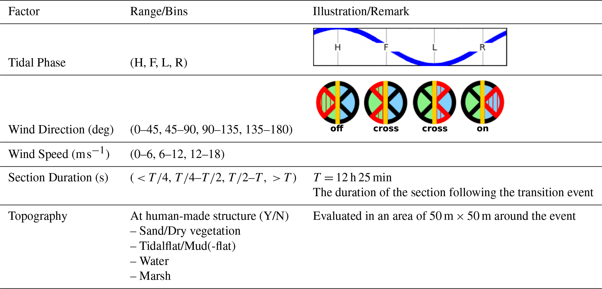
Table 3 Environmental factors and other characteristics chosen to classify transition events. The two illustrations in the right column indicate the local tidal phase and wind direction relative to the shoreline.

Similar arguments can be made for the choice of A_th, but the dependencies of sampling accuracy, frequency, regularity, and the movements of the drifter are more complex. An order estimation for a characteristic reorientation of floating drifters comes from assuming that the travel direction is reversed during falling- and rising-tide phases, such that $\mathrm{180}\mathit{°}/n\left(\mathrm{3}\mathrm{h}\right)\le A_{\text{th}}$, with the average number of samples n(3 h) during 3 h. A useful reference to set this threshold can be derived from the assumption that the changes in direction of a GNSS receiver at rest follow a uniform random distribution: For a set of random variables $\mathit{\{}{a}_i{\mathit{\}}}_{i=\mathrm{0},\mathrm{1},\mathrm{\dots }}\sim \text{Unif}[-\mathrm{180},\mathrm{180}]$ and with the probability $p=\mathbb{P}[{\mathit{\theta }}_p=(\mathrm{1}-p)\cdot \mathrm{180}\mathit{°}\le |a_{\mathrm{0}}\left|\right]$ it follows that $p=\mathbb{P}[{\mathit{\theta }}_p\le A{|}_{\mathit{\left\{}{a}_{\mathrm{0}}\mathit{\right\}}}]$ for one angle. In accordance with the choice of the previous paragraph of one standard deviation for the threshold of the displacement D_th, a lower bound for this threshold is thus $p=\mathrm{0.68}\to {\mathit{\theta }}_{\mathrm{0.68}}=\mathrm{57.6}\mathit{°}\le A_{\text{th}}$. On the other hand, the expected value of the metric $\mathbb{E}\left[A{|}_{\mathit{\{}{a}_{\mathrm{0}},a_{\mathrm{1}},\mathrm{\dots }\mathit{\}}}\right]$ = 90° is independent of the number of samples in each time-window, providing an upper bound. It was found that setting A_th = 58° resulted in satisfactory results.

2.2.5 Evaluation of the Grounded Statistic

Two metrics are used to quantify the agreement of the manually observed groundings with the predictions from the grounded statistic. The first metric makes a comparison for each entry in each time-series. While this approach shows the fraction of correct and incorrect predictions on a time-step basis, it does not indicate the effectiveness of the statistic to identify individual floating and grounded sections. These vary greatly in duration, such that misidentified shorter sections are less apparent. Furthermore, some sections have durations smaller than the chosen time-window and therefore lie outside the scope of the statistic. For these reasons, a second metric is used that compares observations and predictions on a section basis. When examining a recorded trajectory for groundings, sections where the drifter is afloat should have no indication of grounding for the entire duration, and sections where the drifter is on land should have at least one indication of grounding. For this reason, the second metric counts floating sections with the absence of any grounding prediction as one correct floating prediction, and otherwise counts the number of separate subsections of false grounding indications as wrong floating predictions. A grounded section counts as one correct grounding prediction if the grounding is indicated at least once, and as one incorrect grounding prediction otherwise. Sections with durations smaller than ΔT are not taken into account.

The reliability and adaptability of the grounded statistic is evaluated for different re-samplings of the trajectories. The entries were either selected with a uniform stride, or by dropping a fraction of the entries at random. For either method, the number of entries was repeatedly divided by two, in parallel to the reduction of the time-window for the grounding detection. This results in the average number of entries in the time-windows used for the evaluation being similar for different reductions of the trajectory and/or time-window.

2.2.6 Characterization of Grounding and Resuspension Events

We want to identify environmental conditions and other factors that explain the manually observed groundings and resuspensions, where we focus on the situation that a drifter is already in a region where groundings can occur. Since the events happen at the intersection between the water surface and coast, we consider the changes in water level over time in combination with the bathymetry as a proxy for water depth, which in turn informs near coast surface currents, and whether an intertidal zone is flooded or not. Local wind also impacts both the water surface and drifter movements (de Amorim et al., 2025).

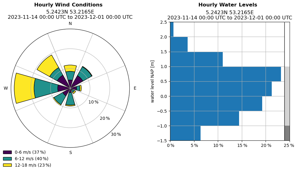
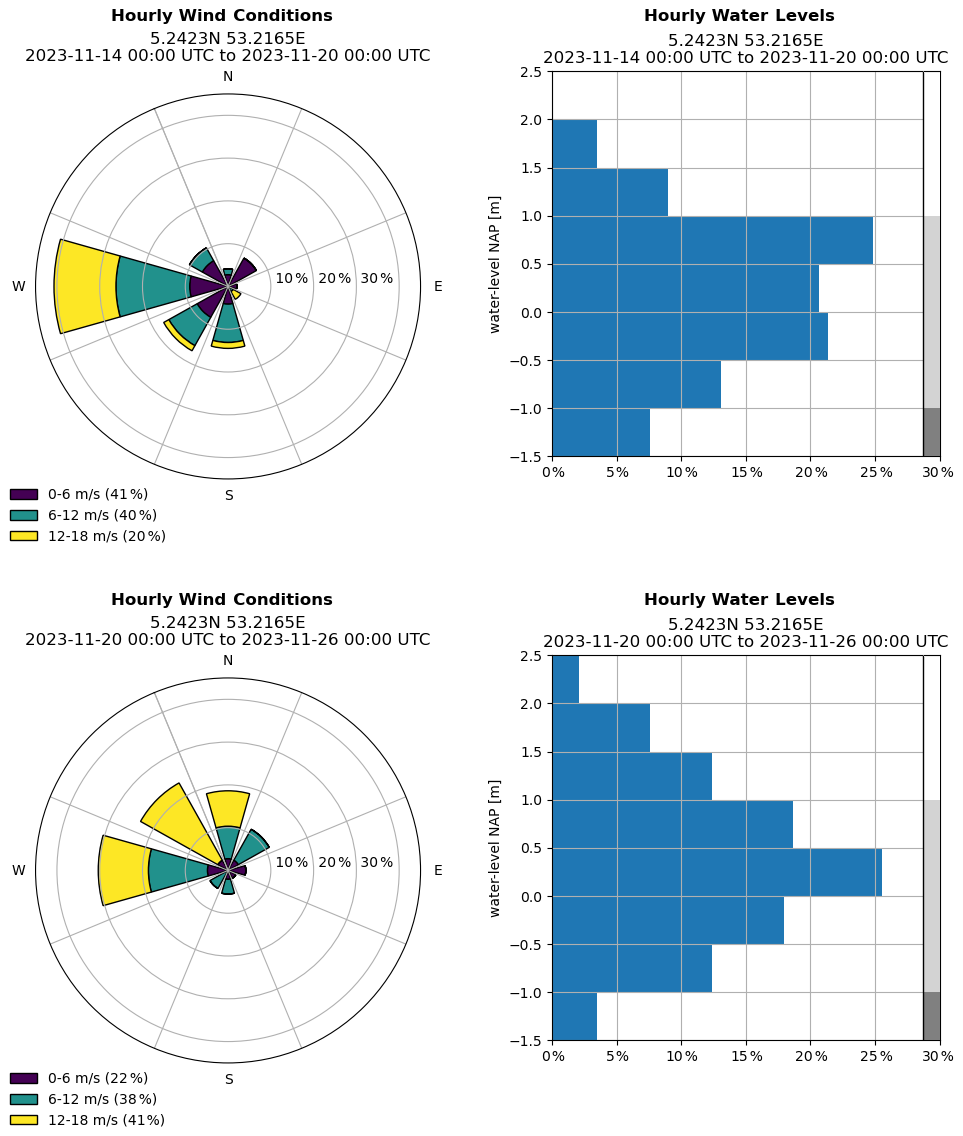
Figure 3 Histograms of hourly wind conditions and water levels from 14 November until 1 December 2023, at the central sampling position marked in Fig. 1. The gray-scale at the right border of the water level histogram is used in the bathymetry map in Fig. 1. Additional statistics are shown in Fig. A5.

Since tides are the main drivers of dynamic changes in the Wadden Sea, we extract the tidal phase from the M2 constituent of the 48 h water level time series at an event location. This is to determine whether an event happens during high, falling, low or rising tides. Wind is characterized by its speed and its direction with respect to the local shoreline orientation of the coast or mudflat. Since determining this orientation appropriately is challenging, we describe our approach and a sensitivity analysis in Appendix C. We separate the local wind direction into four sectors of directly towards shore, diagonally towards shore, diagonally from shore and directly from shore. The observed groundings occurred on slopes with a large variation of directions, which is why we do not differentiate between the two mirrored wind directions with the same angle to the shore. Furthermore, we determine the duration of the sections that follow each transition. Lastly, since the Wadden Sea area and its coast comprise of different landscapes and human-made structures, we also derive a topographical categorization of the areas where the transitions occurred. We first determine whether an event is or is not located within 50 m of a human-made structure. We then further separate the event surroundings by determining one predominant topographical feature per event. Table 3 summarizes the factors we choose for the analysis.

Since we use the manual coding of the transition events for the characterization, this analysis is independent from the grounded statistic. While transition events can be extracted from a time-series where the statistic is evaluated for each time-step of the trajectories, the statistic is designed to indicate the occurrence of grounded sections rather than to identify transitions.

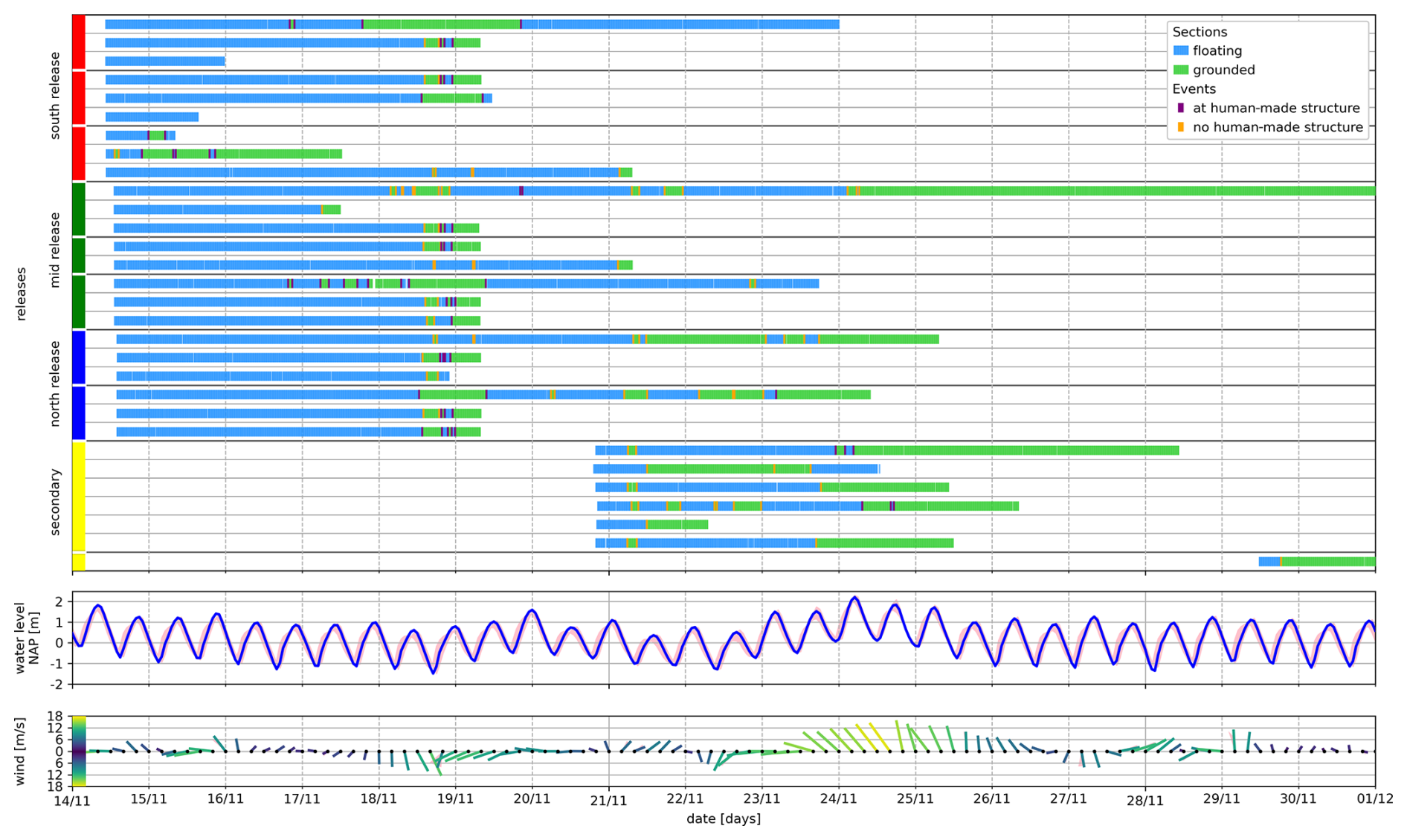
Figure 4 Timelines summarizing the campaign. The upper panel shows for each release the sections and events. The timeline is cut off before the end of two recordings from drifters that remain grounded after 30 November. The colors of the markings at the beginning of the release timeline are matched with the colors of the trajectories in Fig. 1, and white lines separate the primary releases with respect to the nested triangular pattern at each location. The middle and lower panels show the water level (hourly) and wind conditions (4 h increments) for the same time period. Wind strength and direction are illustrated by color, length and orientation of each marker. Both wind and water level are sampled at the three positions shown in Fig. 1, where the values of the central position are show in the foreground, and the values of the NW and SE positions define the bands of variation shown in the background. A simplified vector graphics rendering of this figure is provided in Fig. S2 in the Supplement.

3 Results

3.1 Campaign Overview

The campaign is summarized in Fig. 1 with all trajectories and transition events, Fig. 3 showing the wind conditions and water level during the campaign, and Fig. 4 with timelines of the drifting sections, water level and wind conditions. While the water level timeline shows the dominant component of the semi-diurnal tides, one can also see longer-term trends that persist over multiple days. Wind conditions evolved on time scales of one to a few days. Appendix A contains variations of Fig. 1 with detailed information for each release group, and additional statistics of the wind conditions and water level.

All recoded trajectories and groundings occurred during a few weeks within the Wadden Sea. Only a few drifters transitioned into the North Sea and eventually grounded on a Wadden island. We observe a clear tendency for the drifters to move north-westwards from their release positions. This north-westward drift aligns with the prevailing wind directions, general circulation pattern of the North Sea around the Wadden Sea, and previous findings on transportation patterns in the region (Fajardo-Urbina et al., 2023; Meyerjürgens et al., 2019). Since (Stokes-) drifters are specifically known to be pushed by wind (Medina-Rubio et al., 2026), the containment in the Wadden region of this campaign is at least partially imposed by the evolution of wind conditions. Inside the Wadden Sea, the trajectories visibly correlate with the bathymetry. Inlets and their channels that reach towards the center of the Wadden Sea are accumulation regions for the floating drifters, which is apparent for example at the southernmost inlet Marsdiep south of Texel, whose channel was sampled most densely. The currents resulting from the bathymetry are co-determined by the semidiurnal tides, which predominantly drive the motion of the drifters at the daily timescale. This motion appears in the form of regular oscillations aligned with the M2 tidal signal. The timescale of M2 is also fitting the duration of the observed grounded sections.

We observe in Fig. 4 that the transitions captured in this campaign are a combination of clustered and isolated events. Two clusterings of grounding events occurred in the afternoon of 18 November 2023 and in the morning of 21 November. The number of events associated with either of these clusterings is about one order below the total of 151 observations, such that they make up a significant part to the characterization statistics. The statistics are thus correlated with these clusterings.

The first clustering on 18 November involves 11 drifters from all three primary release locations that get grounded at Vlieland at the 1.5 km long coast strip of Oost-Vlieland within approximately four hours. These drifters accumulate in the south-east of Vlieland at 53.2° N, 5.15° E at low tide in the morning of 18 November. During the following hours, the raising water level coincides with strong south-southeasterly wind, and the drifters move away from the channel of the inlet Vlie towards the coast of Vlieland, where they ground in the afternoon during low tide. Most drifters are shortly re-floated after the first grounding, and the cluster accumulates at the dock wall of the port of Vlieland by the morning of 19 November.

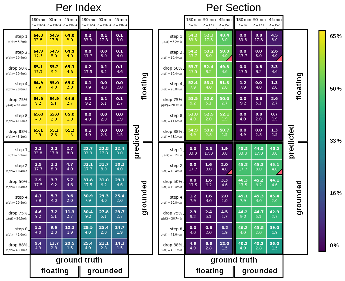
Figure 5 Collection of confusion matrices based on the two metrics of Sect. 2.2.5 and for different re-samplings of all drifter time-series. The horizontal direction lists the time-windows for the grounding detection, together with the total number of comparisons n. The vertical direction lists the resampled time-series, together with the mean sampling interval μ(dt). For each selection of a time-window and a time-series, there is one square in each of the four quarters (separated by black borders) with the matching time-window and time-series labels. These four squares together form the 2 × 2 confusion matrix, such that their bold values add up to 100 %. One example for the metric “Per Section” and choice “45 min” and “step 2” is marked with red triangles in the bottom right corners of the four corresponding squares. In each square, the upper bold number shows the percentage of comparisons classified in the corresponding category, and the lower number shows the mean number of positions contained in the time-windows for the given resampled time-series.

In contrast to this very localized occurrence, the second clustering on 21 November involves nine drifters from the primary and secondary releases, where the groundings occur individually or in small groups at distinctly different locations. These nine groundings include four at the coast facing the North Sea, of which two are located in the east and one in the west of Schiermonnikoog, and one is located in the west of Texel. While the three groundings on Schiermonnikoog commonly follow a similar pattern of inverting from a eastward to a westward direction, each drifter originates from a different primary release location. The trajectory for the grounding on Texel displays a different pattern that is aligned with the Marsdiep inlet. A further group contains three groundings that lie closely together within an area of 200 m on a mudflat in the south of Vlieland. These drifters all originate from a simultaneous secondary release roughly half a day before these groundings, which are thus strongly correlated. The last two groundings are individual and are both located north of Terschelling on mudflats, but separated by multiple kilometers, with trajectories displaying different patterns, and the drifters originate from a primary and a secondary release. Since the trajectories preceding these nine groundings are different in nature, it is challenging to summarize this occurrence beyond the fact that the groundings occur during the same transition from high to low tide.

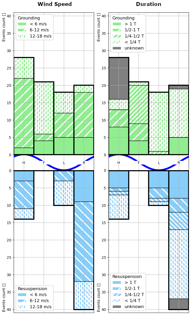
Figure 6 Grounding (upper half) and resuspension (lower half) occurrences with respect to the tidal phase (High, Falling, Low, Rising), and separated by the duration of the following section (right) or wind speed (left). Events where the duration of the following section cannot be categorized are marked gray.

3.2 Evaluation of the Grounded Statistic

We use the metrics and resampling-scheme of Sect. 2.2.5, and the parametrization according to Sect. 2.2.4 to compare the grounded statistic with the manual codings of Sect. 2.2.1. Figure 5 shows a collection of confusion matrices that test the accuracy of the classification into “grounded” and “floating” classes. Each individual confusion matrix results from first choosing a resampling strategy for the trajectories, a time-window for the grounded statistic, and a metric for the comparison. The next step is resampling the trajectories, then evaluating the grounded statistic to create the predictions, and then comparing these predictions with the ground truth values from the manual coding. The four entries of each confusion matrix are separated and grouped with the corresponding entries of the other matrices, and this is done per metric.

We find that predictions based on eight or more positions are correct up to a few percent, and the accuracy based on four positions remains above 90 %. The number of correct classifications tends to be reduced by a few percent when either the mean number of entries that are available for each prediction are reduced from multiple tens down to only a few, or when evaluating irregularly instead of uniformly sampled trajectories. False grounded predictions generally occur more frequently than false floating predictions. This tendency may be intrinsic to the grounded statistic or result from the chosen parameter values.

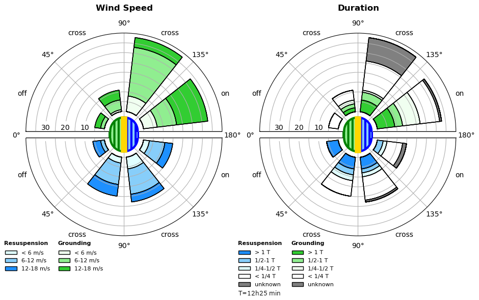
Figure 7 Grounding (upper hemisphere) and resuspension (lower hemisphere) occurrences with respect to the wind direction along the local shore orientation, and separated by the duration of the following section (right) or wind speed (left). Events where the duration of the following section cannot be categorized are marked gray. Land-shore-water orientation is illustrated in the center, and the wind orientation is indicated as the direction from each sector towards the center, as detailed in Table 3: The counts in each sector are including the events of the sector mirrored along the horizontal axis, giving rise to the notion of the four wind directions “directly towards”, “diagonally towards”, “diagonally from” and “directly from” shore.

The results of Fig. 5 may include biases that originate from the observations and choice of parameters that are specific to the campaign, such as from the central impact of tidal cycles on the trajectories and the choice of parameter values. While we observe some synchronization of the drifter trajectories, such as the two clusterings of grounding and resuspension events described in Sect. 3.1, it is unclear if this introduces biases in the results. This is because the clustered events still locally occur over a spatial and temporal range that makes the transitions appear unique with respect to the grounded statistic, and because the grounded statistic applies to subsections of individual trajectories, which implies that there is no direct dependence of co-occurrences of transition events.

3.3 Characterization of Groundings and Resuspensions

Putting the observed events in relation to the tidal cycle in Fig. 6 shows that resuspensions occurred predominantly during rising tides and are absent during falling tides, whilst groundings are much more uniformly distributed. While this outcome for resuspensions seems intuitively correct, the less expected distribution for grounding events can be better understood when also taking the duration of the grounded sections into account: Groundings during low and rising tides are most often short-term, less than one quarter of a tidal cycle. One can observe a shift in the typical duration of grounding events from long-term groundings during high and falling tides to shorter events during low and rising tides.

Separating the events by the local wind direction in Fig. 7 shows that the majority of transitions occur during winds towards shore. For groundings, this asymmetry is more pronounced than it is for resuspensions. Furthermore, only long-term floating sections and short-term grounded sections occurred during off-shore wind, whereas in contrast all resuspension events during on-shore wind are followed by a floating section with a duration of at most one tidal cycle. As for wind strength, the analysis shows that most events occur during median to strong winds (6–18 m s⁻¹). This suggests a non-uniform relation with the abundance of wind conditions during the campaign shown in Fig. 3.

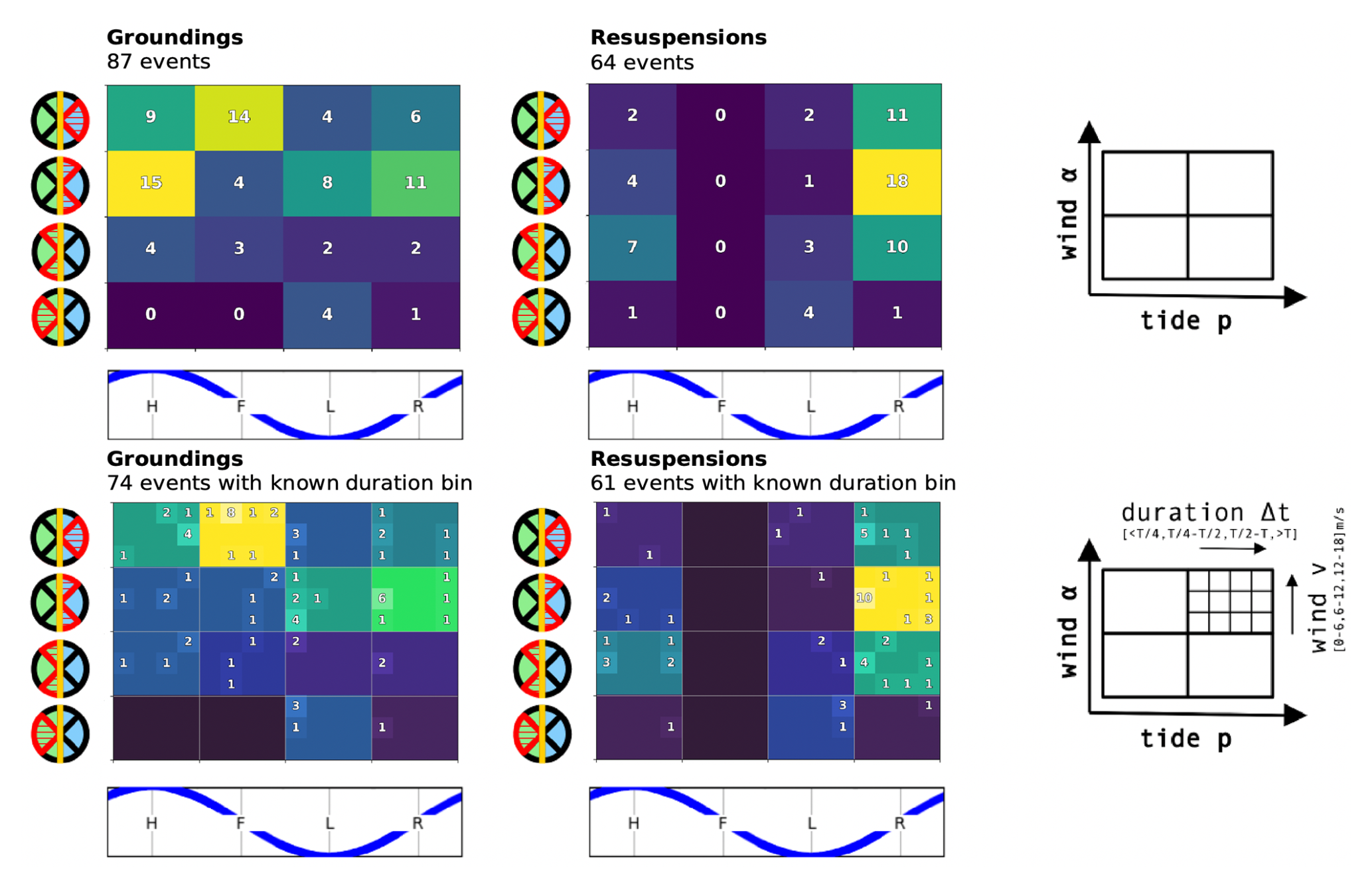
Figure 8 Grounding (left) and resuspension (right) occurrences, separated by the environmental factors summarized in Table 3. The right column illustrates the internal organization of the plots: The upper row shows the counts of events per tidal phase and wind direction, as illustrated in the diagrams of the axes. The lower row further details the counts by also separating them by wind speed and by section duration after each event. Events where the duration of the following section cannot be categorized are excluded in the lower row.

Categorizing the events by both the tidal cycle and wind direction in Fig. 8 shows that most observations can be explained by the following statements: Resuspensions are most often correlated with rising tides, and cross-shore or onshore winds. The occurrence of groundings is often correlated with diagonally or directly on-shore wind.

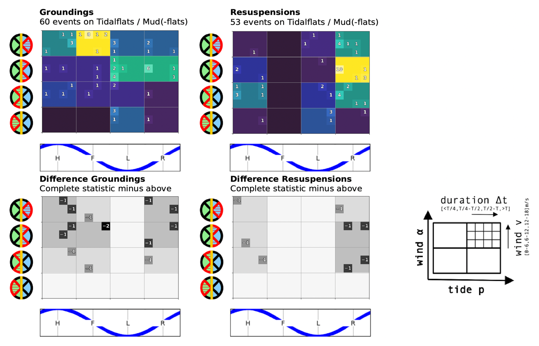
We find that the majority (84 %) of the transitions occurred on tidalflats, mudflats or mud. Since this is comparable to the total number of observations, we include a statistic for these transitions only in Appendix A. There does not appear to be a qualitative change in the characterizations from making this selection. Furthermore, about 60 % of all events occurred in the absence of human-made structures, and 40 % occurred within 50 m of human-made structures that border the water. Since the clustering of 11 drifters on 18 November mentioned in Sect. 3.1 occurred in an area where the drifters were close to human-made structures, we expect a dominant correlation between this clustering and statistics about events at such structures. For this reason, we don't include a comparison between transitions in the presence and absence of human-made structures here.

4 Conclusions

We report a campaign in the Dutch Wadden Sea with 24 surface drifters where we identify 151 events related to groundings. In addition to manually coding the recorded trajectories, we also describe a statistical approach that indicates sections where the drifters are grounded. This statistic relies on four parameters that define the minimum duration of a detectable section, and the sensitivity to inaccuracies of the position measurements. While their values can be inferred from the sampling rate and measurement accuracy, physical arguments of the observed water body provide insights about which kind of phenomenon can be resolved. We evaluate how reliably the statistic indicates the occurrence of groundings, and demonstrate that it is robust to changes in the average number of entries and irregular sampling. A potential continuation for the statistical examination of groundings is to also automatically locate transition events in trajectories.

We characterize the observed grounding and resuspension events with five factors: The tidal phase, the wind direction and speed, the duration of the subsequent sections, and the surrounding topography. Roughly 84 % of all transitions occurred on tidalflats, mudflats or mud, and 40 % of the total at human-made structures. We find that both resuspensions and groundings occur rarely during off-shore wind, resuspensions were not observed during falling tides but often during rising tides, and while the number of groundings is much more uniformly spread over tidal cycles, the durations of grounded sections are shorter the closer the corresponding grounding happens before rising tides. These general observations agree with our intuition about grounding processes, which confirms the correctness of the analysis. The grounding characterization may be refined by including processes such as surges and neap-spring tidal cycles.

The identified factors and detailed statistics provide a reference for future marine plastic modeling and beach cleanup efforts, where models or weather forecasts can be used to estimate groundings and abundance of macroplastic at the coast. We find that mean to strong winds (6–18 m s⁻¹) directed towards shore, and the time-window before and up to low tide favor the accumulation of grounded drifters. On the contrary, many resuspensions occur during cross shore wind, and before or up to high tide.

We identify clusterings in the observed events that involve in the order of one tenth of all observations. These clusterings are thus correlated with the characterization statistics. The two clusterings that involve the largest numbers of events differ vastly with respect to the area in which they occur. While one is localized within a few kilometers at the coast of an island, the other is a timely synchronized accumulation of transitions that occur at the Wadden Sea and North Sea coast in small groups that are separated by multiple 10 to 100 km.

Our results are specific to the flat shape and relatively heavy weight of the Stokes Drifters. In contrast, marine macroplastics have widely varying shapes, weights and air-to-water drag ratios, which impacts their dynamical behavior. Putting this study into context with other objects, or deriving a corrective statistic to account for this specificity of the campaign can thus further improve the understanding of the grounding patterns of macroplastic.

A further limitation is that our observations and results apply for the conditions of the campaign. The drifters were in the water during prevailing westerly wind, and the occurring water levels and currents are heavily impacted by wind and semidiurnal tidal cycles. The complex topography and hydrodynamics of the Wadden Sea gives rise to multiple intertwined temporal and spatial scales. While this is an opportunity to study groundings under a large range of conditions, it also poses the challenge to manage the complexity in the data analysis.

Appendix A: Additional Campaign Characterizations

This section contains detailed versions of the campaign summary in Fig. 1 for the four drifter release groups, and two detailing statistics of the wind-conditions and water levels of Fig. 3. We show in Fig. A1 the southern, in Fig. A2 the central, in Fig. A3 the northern, and in Fig. A4 the secondary releases, and in Fig. A5 the detailed conditions statistics.

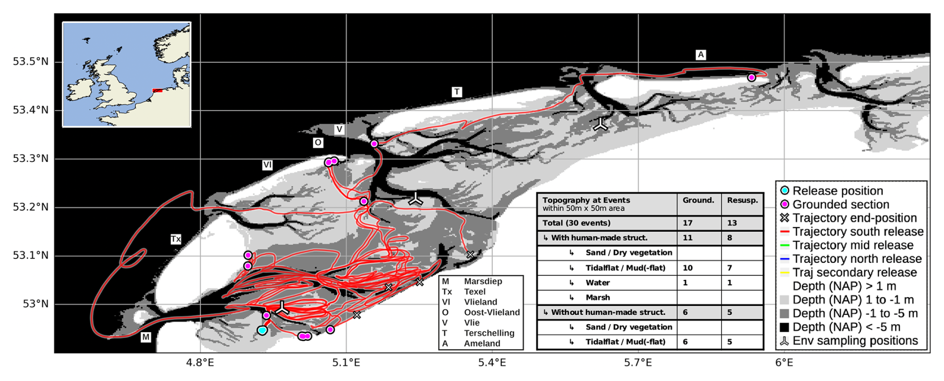
Figure A1 South release renderings and topographic countings detailing Fig. 1. Maps and bathymetry generated with (Map data ©Crown Copyright, Met Office, 2010–2015, licensed under OGL v3.0; Additional layers ©Waddenregister, 2026 (CC-BY 4.0)). A simplified vector graphics rendering of this figure is provided in Fig. S3 in the Supplement.

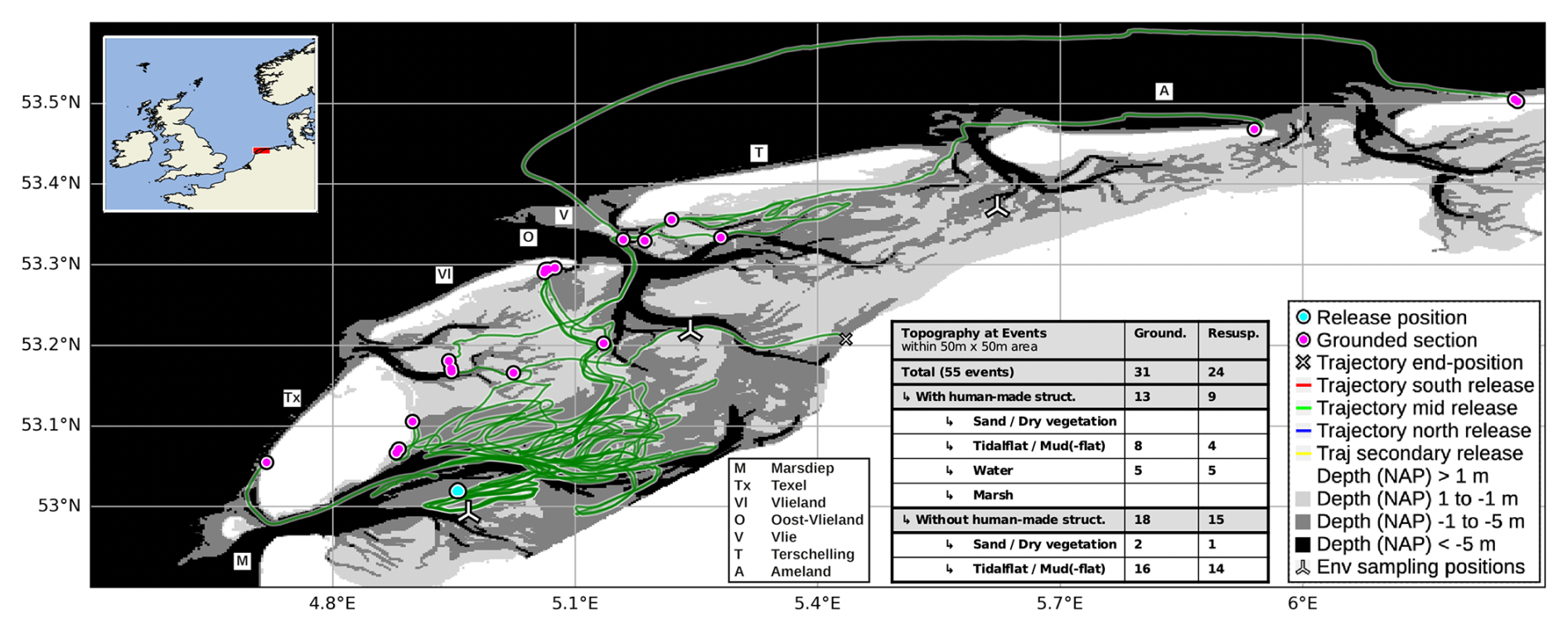
Figure A2 Central release renderings and topographic countings detailing Fig. 1. Maps and bathymetry generated with (Map data ©Crown Copyright, Met Office, 2010–2015, licensed under OGL v3.0; Additional layers ©Waddenregister, 2026 (CC-BY 4.0)). A simplified vector graphics rendering of this figure is provided in Fig. S4 in the Supplement.

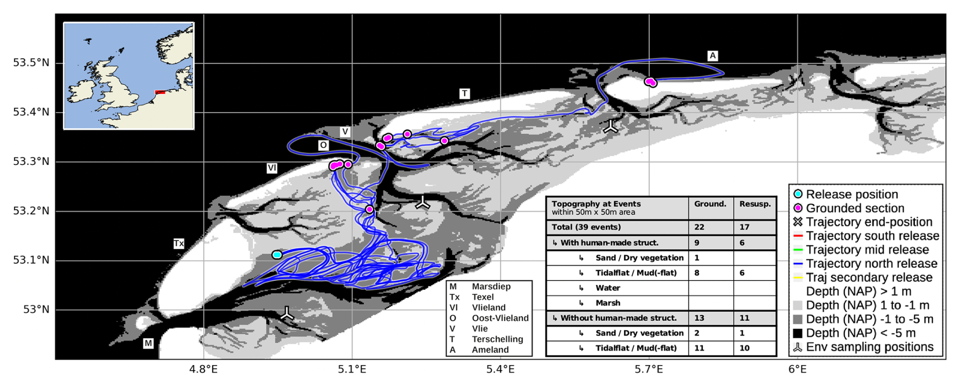
Figure A3 North release renderings and topographic countings detailing Fig. 1. Maps and bathymetry generated with (Map data ©Crown Copyright, Met Office, 2010–2015, licensed under OGL v3.0; Additional layers ©Waddenregister, 2026 (CC-BY 4.0)). A simplified vector graphics rendering of this figure is provided in Fig. S5 in the Supplement.

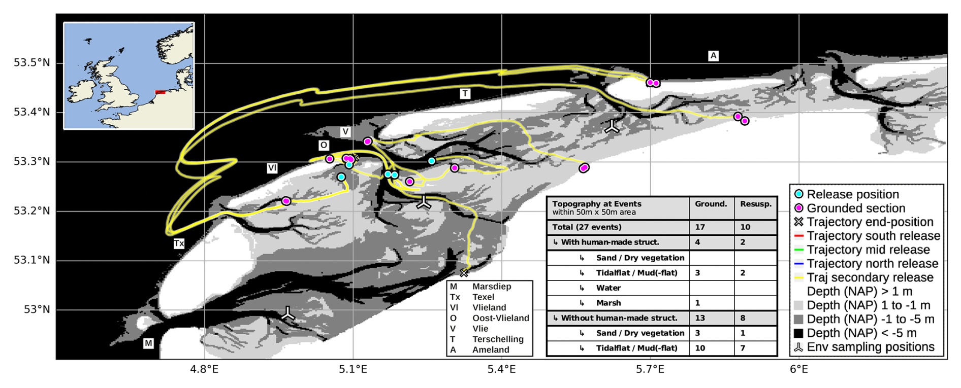
Figure A4 Secondary release renderings and topographic countings detailing Fig. 1. Maps and bathymetry generated with (Map data ©Crown Copyright, Met Office, 2010–2015, licensed under OGL v3.0; Additional layers ©Waddenregister, 2026 (CC-BY 4.0)). A simplified vector graphics rendering of this figure is provided in Fig. S6 in the Supplement.

Figure A5 Additional histograms of hourly wind conditions and water levels at the central sampling position marked in Fig. 1. The two time-windows used here are subsets of the one used in Fig. 3. They are chosen based on groupings of floating sections visible in the timelines of Fig. 4.

Appendix B: Additional Groundings Characterizations

Since the majority of events occurred on tidal- or mudflats, we include here the statistic for these events only in Fig. B1.

Figure B1 The same evaluation of grounding (left) and resuspension (right) occurrences as in Fig. 8, but only for events on tidal- or mudflats (top) and the comparison to the complete statistic (bottom).

Appendix C: Sensitivity Analysis for the Local Wind Direction

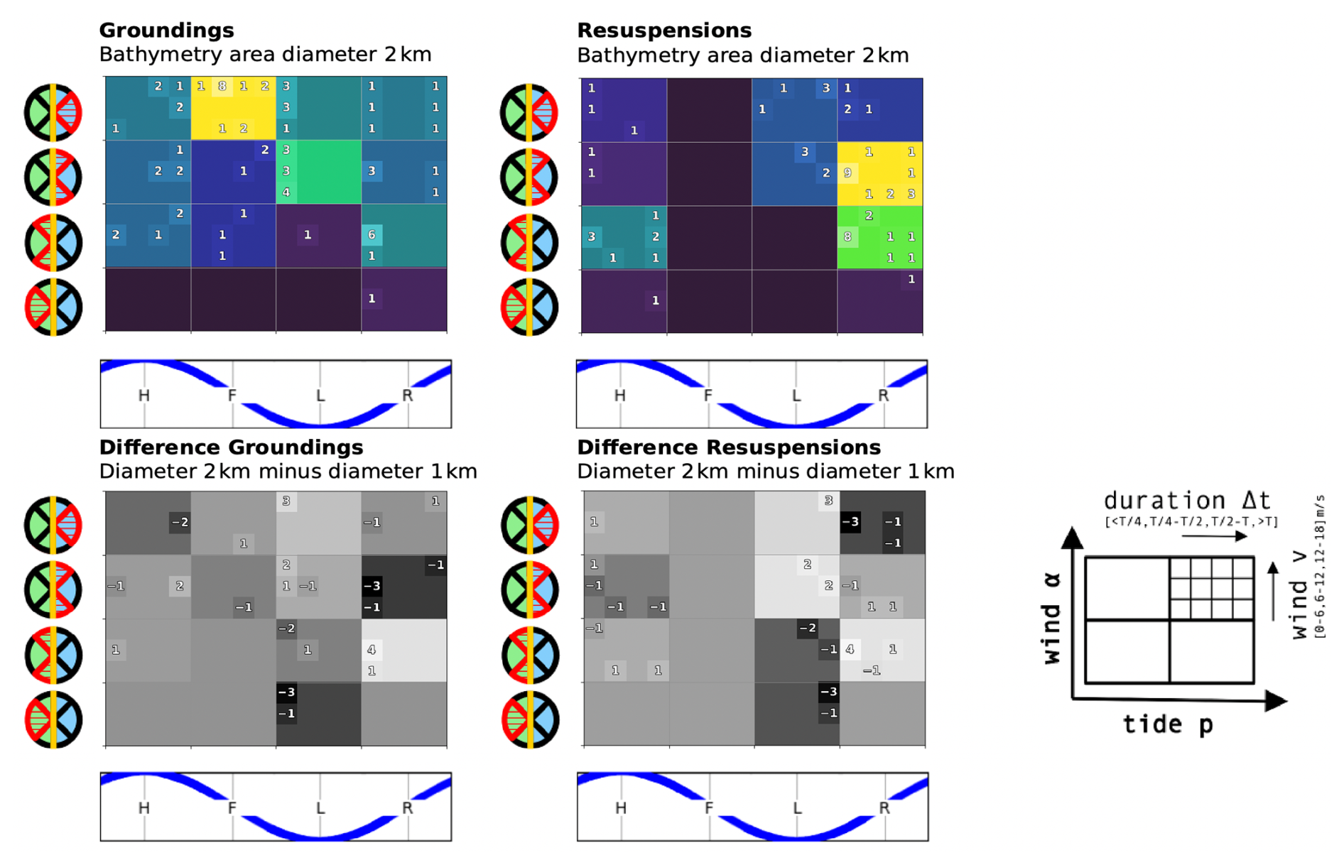
The local wind direction at grounding sites is determined by computing the shoreline orientation of the coast or mudflat from the bathymetry map (Waddenregister, 2026) and determining the wind direction with respect to this orientation (ERA5, 2026). The shoreline orientation is computed by fitting a plane to the bathymetry values at the grounding location that lie within a given radius. The orientation of the plane then determines the shore orientation. The bathymetry map of the Wadden Sea resolves objects on multiple length-scales, and the dynamics of the grounding events are impacted by water movement that also involves multiple length-scales. It is thus difficult to select a radius for the computation. For this reason, Figs. C1 and C2 contain a sensitivity analysis with choices of 0.5 and 2 km for the radius, instead of the 1 km used for the main analysis of Fig. 8. The lower boundary of 0.5 km still includes multiple values of the bathymetry map that has a resolution of 0.1 km, and the upper boundary of 2 km coincides with larger topographic features like the minimum width of some of the islands.

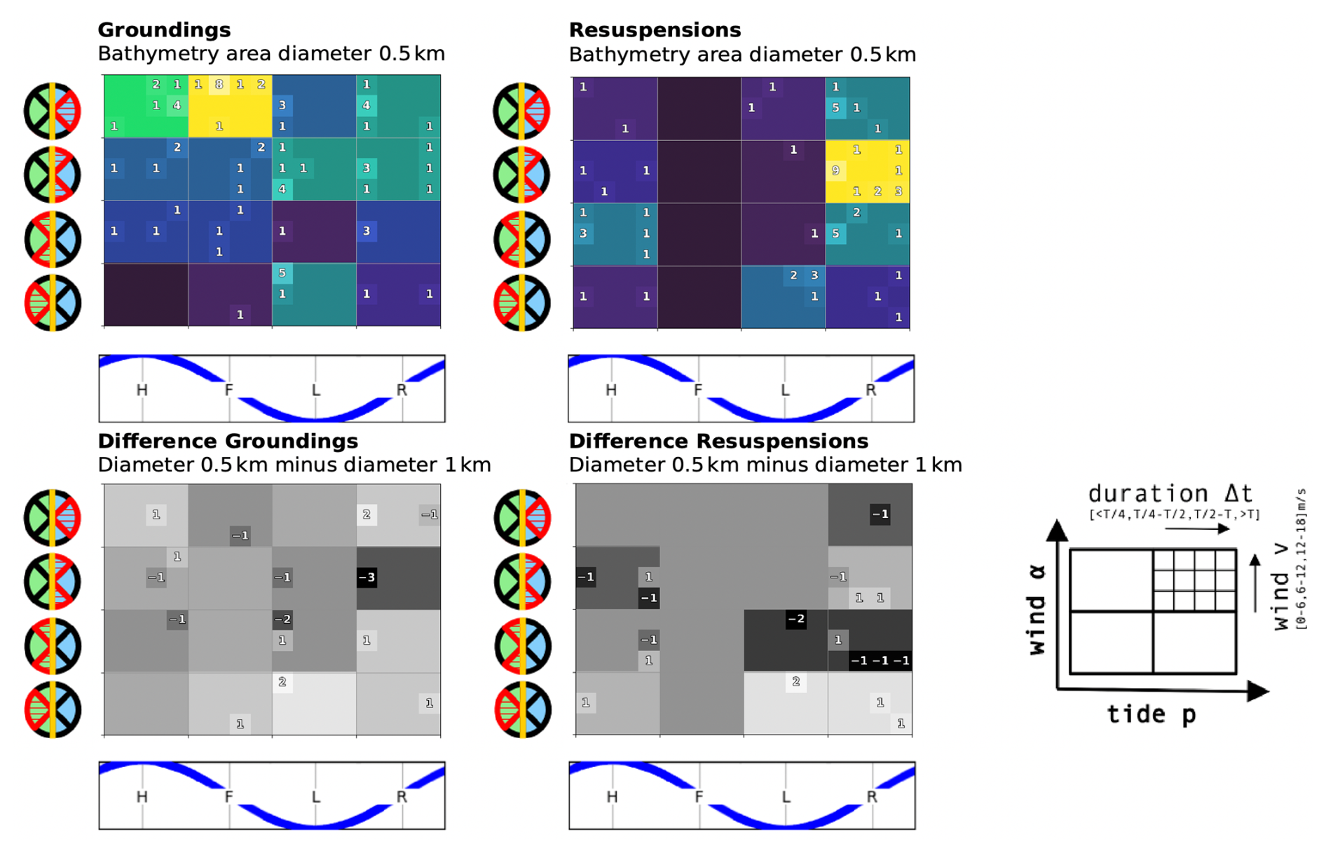
Figure C1 Sensitivity analysis for the computation of the local shoreline orientation at the grounding sites. The plots here show the results for a radius of 0.5 km (top) and the difference to the results for a radius of 1 km (bottom) used in the main analysis of Fig. 8.

Figure C2 Sensitivity analysis for the computation of the local shoreline orientation at the grounding sites. The plots here show the results for a radius of 2 km (top) and the difference to the results for a radius of 1 km (bottom) used in the main analysis of Fig. 8.

Appendix D: Description of the Manual Identification of Grounding and Resuspension Events

The drifter trajectories were inspected visually with plots that display the water level and bathymetry as shown in Fig. D1. We define the following terms to describe the labeling of drifter trajectories:

• A point p_i is a position in the scatter plot of the trajectory. The points are marked as small circles with a white interior and black border.

• A step $s_i=(p_i,p_{i+\mathrm{1}})$ consists of two successive points in the scatter plot, connected by a white line with a black border.

• A trajectory $(p_{\mathrm{0}},\mathrm{\dots },p_N)$ is a succession of all position measurements for one drifter release

• The direction of displacement is the consistent direction of displacement during about three successive steps.

• The jitter is the random displacement that appears as star-like pattern of successive positions in the plot.

The grounding and resuspension events are then identified as described in Table D1.

Table D1 Identification criteria for grounding events.

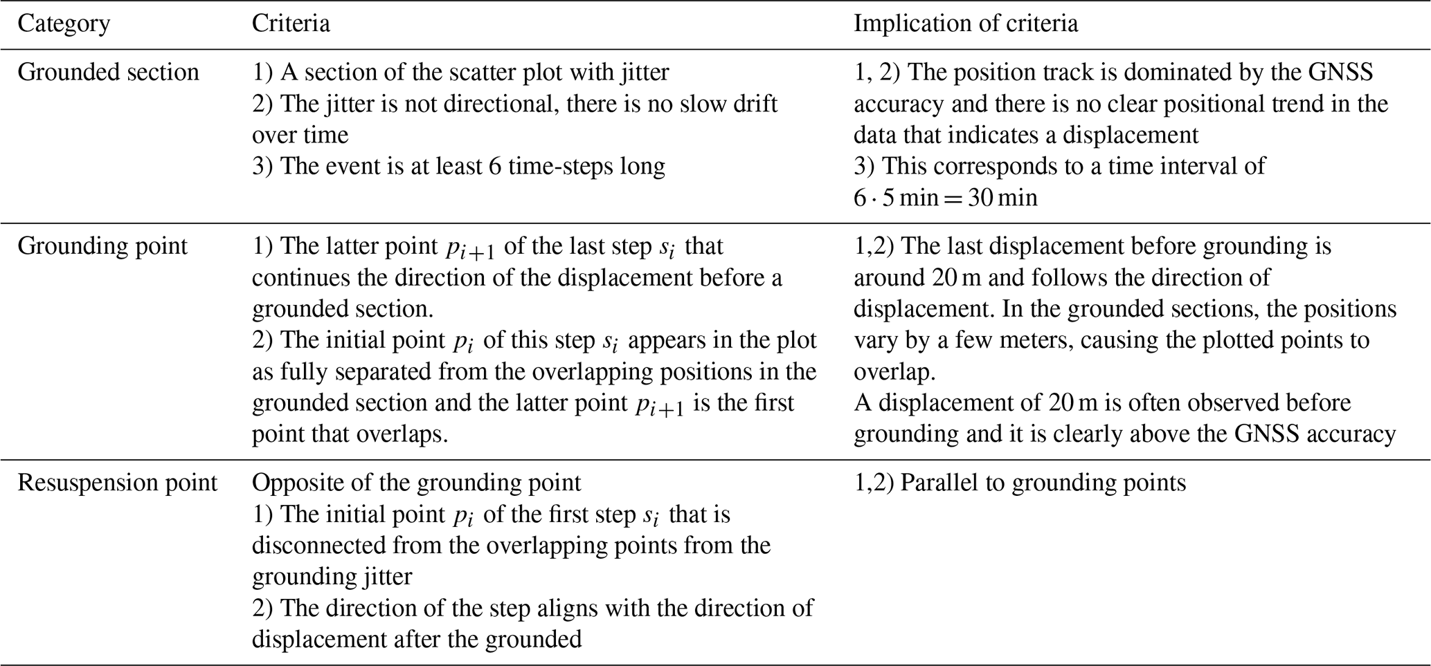
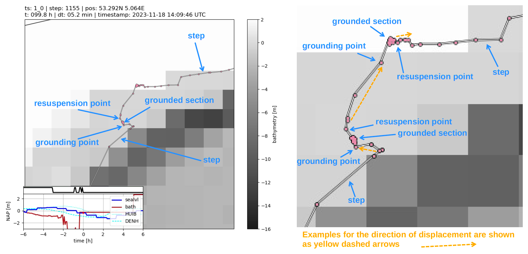
Figure D1 Trajectory plots for manual labeling with added annotations in orange (left) and a zoom-in of the same trajectory with more detailed annotations (right). Maps and bathymetry generated with (© Waddenregister, 2026 (CC-BY 4.0)).

Appendix E: Standardized Directional Change Computation

The recorded changes in position of GNSS receivers at rest are frequently at the resolution scale of the data, such that positions often only change by a fixed minimal value increment along the North or East direction. An example of this can be seen in the insert of Fig. 2. This happens sporadically and creates a substantial number of directional changes that fall precisely on multiples of 90°. We assume that this behavior varies for different receiver and logging solutions, and that asserting uniformly scattered directional changes is more universal. For this reason, we compute the directional changes α(t_i) from the recorded positions augmented with unbiased normal noise at a noise-level of the standard deviation of the GNSS receiver accuracy σ_gnss

$$\begin{array}{ll}{\displaystyle }& {\displaystyle }\mathit{\alpha }\left(t_{\mathrm{i}}\right):=\mathrm{\measuredangle }\left(p\right(t_{i+\mathrm{1}})-p(t_{\mathrm{i}})+\mathit{ϵ}(t_{i+\mathrm{1}}),p(t_{\mathrm{i}})-p(t_{i-\mathrm{1}})+\mathit{ϵ}(t_{\mathrm{i}}\left)\right),\\ {\displaystyle }& {\displaystyle }\text{with }\mathit{ϵ}\sim \mathcal{N}\left(\right[\mathrm{0},\mathrm{0}],{\mathbb{1}}_{\text{2x2}}\cdot {\mathit{\sigma }}_{\text{gnss}}^{\mathrm{2}}).\end{array}$$

This increases the standard deviation of a position recorded at rest by a factor of 1.4, which in our case lies below the scales that we rely on for the data analysis. Furthermore, this noise is only applied for the computation of the changes in directions. For the analysis here, we determine σ_gnss from the trajectory of a drifter at rest.

Appendix F: Drifter Sticker

Figure F1 Sticker placed on both sides of the Stokes Drifters.