Evaluation of sea ice variability in three ocean reanalyses and two regional models in the Barents and Kara Seas in 1991–2020

Satellite measurements indicate that the Barents and Kara Seas have experienced some of the most significant sea ice declines and increases in sea surface temperature in the Arctic. Understanding the processes driving these changes is of utmost importance to assess the implications of climate change in the Arctic and globally. Given the observational limitations in these high-latitude areas, coupled models and reanalysis products play a key role. However, it is essential to determine how reliably these products represent the observed sea ice decline and mixed-layer warming. Models are often evaluated on a pan-Arctic scale, but the model skill might differ when considering sub-regions. This study examines two coupled regional climate models (HIRHAM–NAOSIM 2.2 and RASM), two regional ocean reanalyses (RARE 1.15.2 and TOPAZ 4B), one global ocean reanalysis (ORAS5), and OSI SAF satellite observations over the period 1991–2020. We focus on spring (March–May) and autumn (August–October) sea ice area and sea ice concentration, the edge of the sea ice, and the temperature of the mixed layer. We also examine correlations between sea ice and mixed-layer temperature anomalies and five climate indices to assess how the datasets respond to large-scale climate variability. The results show a statistically significant decrease in sea ice area and sea ice concentration in the satellite measurements and in all reanalyses. However, HIRHAM–NAOSIM shows only a near-significant decline in the Barents Sea, RASM shows no long-term change, and none of the two models shows a significant trend in the Kara Sea. Additionally, the reanalyses show a more pronounced warming of the mixed layer than the coupled models, particularly in autumn and in the Kara Sea. ORAS5 and TOPAZ agree most closely with the observed sea ice, partly because assimilated observations constrain their historical states, whereas RARE reproduces the decreasing trends but overestimates sea ice and shows anomalous mixed-layer temperature behaviour in the Barents Sea. The reanalyses also represent the relationships with the climate indices more consistently than the coupled models, particularly for the Atlantic Multidecadal Oscillation and the Northern Hemisphere ocean heat content. Among the coupled models, HIRHAM–NAOSIM represents changes in the Barents Sea better than RASM, but in the Kara Sea, where none of the models captures the decreasing trends, RASM has a more realistic mean sea-ice state. Although the coupled models reproduce interannual variability, the results indicate that in particular the effects of large-scale changes of the ocean circulation are not realistically reproduced in the coupled models.

1 Introduction

The Arctic sea ice is an important part of the Arctic Ocean and the global climate system, as it influences ocean circulation and atmospheric processes by regulating the exchanges of moisture, momentum, and heat between the ocean and atmosphere. The reduction of sea ice has been linked to feedback mechanisms (Goosse et al., 2018), leading to Arctic Amplification (Stroeve and Notz, 2018). The two marginal seas that have experienced the largest sea ice decline and surface warming in the Arctic are the Barents and Kara Seas (Årthun et al., 2012; Lind et al., 2018; Onarheim et al., 2018) (Fig. 1). The observed warming trends in this region, along with increased salinity and altered vertical fluxes that lead to reduced stratification, have been associated with intensified Atlantic Water (AW) inflow to the Arctic and with local and regional feedback processes, affecting both physical and ecological systems (Asbjørnsen et al., 2020; Ingvaldsen et al., 2021). These observed changes characterise the region as a warming hotspot (Lind et al., 2018) and as a mediator of climate change between the North Atlantic and the central Arctic basins (Smedsrud et al., 2013).

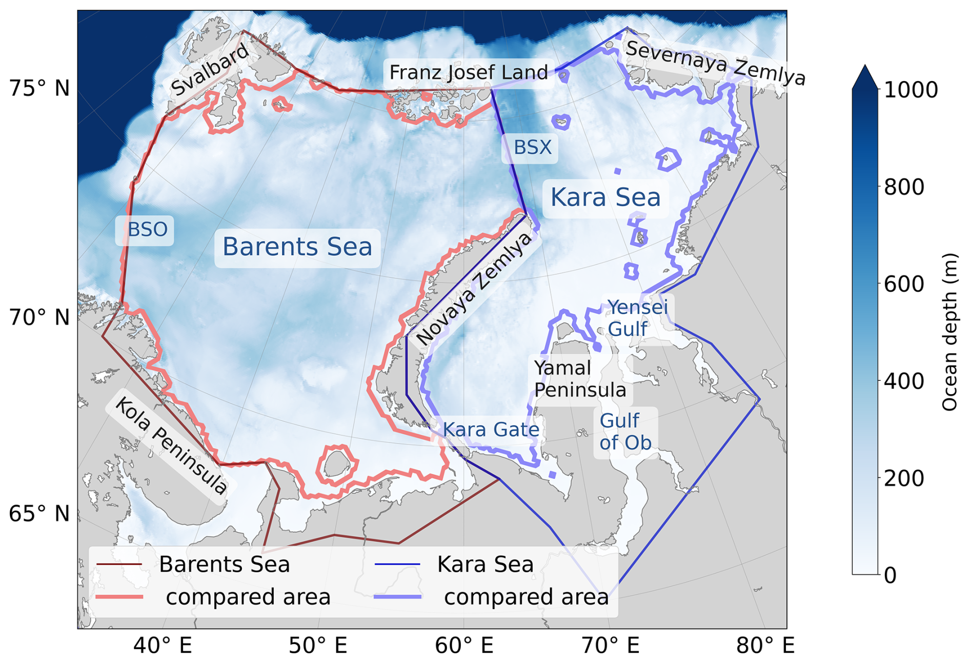
Figure 1 Barents and Kara Seas bathymetry, International Hydrographic Organization domains (darker lines; International Hydrographic Organization and Sieger, 2012), and regions with data available in all models (lighter lines), which are used for area-averaged comparisons. BSO stands for Barents Sea opening and BSX for Barents Sea exit. Bathymetric data from GEBCO Bathymetric Compilation Group (2026).

The Barents and Kara Seas are shallow marginal seas of the Arctic Ocean located north of Norway and Siberia. The Barents Sea is connected to the Nordic Seas and receives warm Atlantic Water through the Barents Sea Opening (BSO). In contrast, the Kara Sea is rather isolated from the adjacent seas, with Novaya Zemlya in the west as a barrier to the Barents Sea, with inflow through the Barents Sea Exit (BSX) to the north and the shallow and narrow Kara Gate to the south. The mean annual freshwater inflow to the Kara Sea relative to its area is the largest in the world due to the inflow from the Ob, Yenisei, and other large rivers, affecting its stratification and circulation patterns. These seas play distinct roles in the Arctic system – for instance, the role of the Barents Sea as a key gateway between the North Atlantic and the Arctic Ocean (Skagseth et al., 2008; Smedsrud et al., 2013). This has a disproportionately large influence on the Kara Sea landfast ice and on the halocline stability of the Eurasian Basin and beyond, as noted by Liu et al. (2025).

Several studies have looked into the sea‑ice variability in the Barents and/or Kara Seas and the processes behind it (e.g., Duan et al., 2019a; Kumar et al., 2021; Li et al., 2022; Shabanov et al., 2024; Chatterjee et al., 2024; Dörr et al., 2024). Warm Atlantic waters flow into the Barents Sea through the BSO, are progressively modified and lose heat to the atmosphere. Part of this modified water subsequently exits the Barents Sea through the BSX toward the Kara Sea, while Barents Sea waters also enter the Kara Sea through the Kara Gate. Shabanov et al. (2024) found that the strongest trends in Kara Sea ice conditions occur near pathways of Atlantic-water inflow, highlighting the role of Atlantification in the observed sea-ice decline. Several studies have also linked variability in Atlantic heat transport through the BSO to interannual variability in Barents Sea sea ice (e.g., Årthun et al., 2012; Wang et al., 2019). While this oceanic inflow can enhance sea‑ice melt and contribute to Atlantification, atmospheric forcing also plays an important role in sea-ice variability, with air temperature, winds, and radiative fluxes exerting strong control, and can also influence sea ice indirectly by modulating ocean heat transport into the Barents Sea (Duan et al., 2019a; Wang et al., 2019). Recent work provides further evidence that the ocean can be a dominant driver of interannual sea-ice variability in parts of the region. Dörr et al. (2024), for example, found that ocean heat transport dominates in the central and northeastern Barents Sea, whereas atmospheric drivers are more important in the northern Barents and Kara Sea. Overall, the atmosphere, ocean, and sea ice form a tightly coupled system, and internal feedbacks make it difficult to attribute observed variability to any single driver (Duan et al., 2019a; Chatterjee et al., 2024).

Although the Barents and Kara Seas are often studied as a single Barents–Kara region (e.g. Li et al., 2022; Dörr et al., 2024), these marginal seas differ substantially in terms of circulation, stratification, and seasonal sea ice cycle. The Barents Sea is ice-covered in the northern parts in the winter and can become nearly ice-free across the region in summer, whereas the colder Kara Sea is typically fully ice-covered in winter and becomes largely ice-free in summer (Duan et al., 2019a, b). Observed sea ice decline has also been more pronounced in the Barents Sea than in the Kara Sea (Kumar et al., 2021). These differences motivate us to consider the two regions separately.

Advances in the observing and modelling capacities in recent decades have provided tools to widen our understanding of the polar regions. Observations, reanalysis products, and models are complementary tools used to better understand the Arctic climate system, the processes behind recent changes, and its possible future evolution. Nevertheless, existing data products and models present both advantages and disadvantages. Ocean reanalyses combine models and observations via data assimilation; these products give an estimate of the ocean and sea ice (Balmaseda et al., 2015) and are important for studying processes that are only partly or indirectly observed, as well as for initialising and forcing models, but they often struggle in data-sparse regions (Storto et al., 2019). Global Earth system models provide a representation of the whole Earth's climate and possible pathways for the future. However, the resolution of these models is usually too coarse to simulate all interactions and feedback between the components. Docquier et al. (2020) showed that a horizontal resolution of 1°, which is common for the global models, is not sufficient to correctly simulate the ocean currents entering the Arctic through the Barents Sea. Furthermore, they highlight the need for a high horizontal resolution to correctly represent the Arctic sea ice in the models. Coupled regional ocean–atmosphere models offer the ability to better resolve regional processes and the associated feedbacks, in comparison to their global counterparts, due to their finer resolution. These models also offer the ability to respond to real-world changes in the large-scale atmospheric circulation by quasi-observed lateral boundary conditions from reanalysis data.

This paper evaluates several reanalysis products and regional climate models and focuses on assessing their skill in representing observed sea ice and mixed layer temperature in the Barents and Kara Seas. The associated biases and trends in each of these products and models are used to evaluate their strengths and weaknesses. This allows us to provide concrete guidance to users on the appropriate use of such products and models for different purposes. Understanding the performance of reanalysis and models in these regions is crucial due to their role as hotspots in the current Arctic climate change.

2 Reanalysis and regional model data

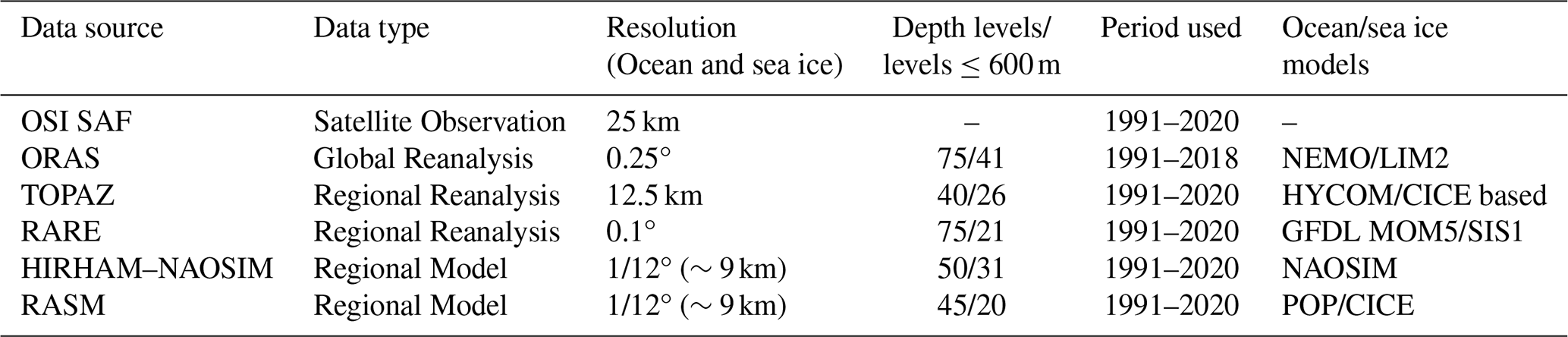
In this study, we evaluate sea ice variability and mixed layer temperature from two coupled regional atmosphere–ocean models, HIRHAM–NAOSIM (Dorn et al., 2019) and RASM (Cassano et al., 2017; Seefeldt et al., 2024), and two regional ocean reanalyses, TOPAZ version 4b (Xie et al., 2017; EU Copernicus Marine Service Information (CMEMS), 2024) and RARE version 1.15.2 (Carton and Chepurin, 2023). The regional products were selected to represent different model components, configurations, and approaches to data assimilation. In particular, the coupled models allow air–sea interactions to evolve within the model system, while the ocean reanalyses are forced by atmospheric reanalysis and observations. The two ocean reanalyses also differ in their treatment of sea ice observations: TOPAZ assimilates satellite sea ice concentration (SIC) observations, whereas RARE does not (Sect. 2.2). We use EUMESAT Ocean and Sea Ice Satellite Application Facility (OSI SAF) SIC data, OSI-450-a (EUMETSAT, 2022), as a comparison point for the sea ice model and reanalysis data. Additionally, we use the global reanalysis ORAS5 (Zuo et al., 2019), a global benchmark known for its good performance (Zuo et al., 2019). ORAS5 is also the source for the ocean boundary conditions in HIRHAM–NAOSIM. ORAS5 is evaluated together with the other reanalyses for the sea ice variables, but is used as the comparison point for the mixed layer (ML) temperature evaluations. The datasets are described below and summarised in Table 1.

Table 1 Datasets used in this study.

2.1 Coupled regional models

HIRHAM–NAOSIM is a coupled regional atmosphere–ocean–sea ice model applied over a circum-Arctic domain using rotated latitude–longitude grids with a horizontal resolution of 1/4° (∼27 km) and 40 vertical layers in the atmosphere component HIRHAM and 1/12° (∼9 km) and 50 vertical layers in the ocean–sea ice component NAOSIM. Detailed information on the model components and their coupling is given by Dorn et al. (2019), and information on the current model version 2.2, particularly regarding recently introduced reparametrizations, is given by Aue et al. (2023) in their supplementary material. The simulation used for the present study was run for the period 1979–2021, with the first part of the simulation disregarded to let the model find its own steady state. The analysis was therefore restricted to the period 1991–2020. It is driven by ERA5 reanalysis data (Hersbach et al., 2020) at HIRHAM's lateral boundaries and at HIRHAM's lower and NAOSIM's upper boundaries, which are not covered by the domain of the other model component. For NAOSIM's open lateral boundaries in the North Atlantic, ORAS5 reanalysis data were used.

The Regional Arctic System Model (RASM) is a fully coupled atmosphere–land-ocean-sea ice model. It uses the Weather Research and Forecasting (WRF; Powers et al., 2017) version 3.71 for atmosphere, a regionally configured version of Parallel Ocean Program (POP; Smith et al., 2010) version 2.1 for the ocean and the Los Alamos National Laboratory Sea Ice Model CICE version 6 (Hunke et al., 2018) for sea ice. Additionally, it uses the Variable Infiltration Capacity (VIC) land hydrology model and the streamflow routing (RVIC; Hamman et al., 2017) model for transporting the freshwater flux from the land to the ocean. The ocean and sea ice have a resolution of 1/12° (∼9 km) on a rotated grid with 45 vertical levels for the ocean and 5 thickness categories for sea ice.

2.2 Ocean reanalysis

The Arctic Ocean physical reanalysis TOPAZ 4B (hereafter TOPAZ) is a regional ocean reanalysis for the polar region north of 50° N (Xie et al., 2017). It uses the Hybrid Coordinate Ocean Model version 2.2 (HYCOM; Chassignet et al., 2003), and a single-category version of CICE 3 for sea ice (Xie and Bertino, 2025). ERA5 data is used as atmospheric forcing. The model uses the deterministic ensemble Kalman filter (DEnKF) to assimilate multiple ocean and sea ice observations simultaneously (Xie et al., 2023), such as SIC and drift from OSI SAF, gridded sea surface temperature (SST) from OSTIA, and in situ temperature and salinity profiles from the CORA database. Additionally, sea ice thickness for the winter months from CS2SMOS and sea surface salinity based on the SMOS satellite are assimilated after 2010. For river runoff, the reanalysis uses a climatology based on ECMWF reanalysis and the TRIP hydrological model (Xie and Bertino, 2025). The data are provided at a standard polar stereographic grid with 12.5 km resolution and 40 depth levels.

The Regional Arctic Reanalysis RARE 1.15.2 (hereafter RARE) is a regional reanalysis with a southern boundary at 44.7° N (Carton and Chepurin, 2023). It uses the GFDL MOM5/SIS1 numerical model and ERA5 as surface forcing. The model assimilates World Ocean Database (WOD) hydrographic profiles as well as satellite and in situ SST profiles (Carton and Chepurin, 2023). Sea ice thickness estimates of the Pan-Arctic Ice Ocean Modeling and Assimilation System 2.1 (PIOMAS; Zhang and Rothrock, 2003) are used to constrain sea ice using a net surface heat flux relaxation term with a 30 d time scale. Areas with thicker sea ice compared to PIOMAS receive more surface heat flux, and thinner areas receive less (Carton and Chepurin, 2023). The continental discharge is based on a dataset combined from the World Meteorological Organisation Global Runoff Data Centre estimates and discharge estimates from R-ArcticNET and the Arctic Great Rivers Observatory; gaps in the dataset are filled with climatological monthly estimates. The dataset is provided on a regular 0.1° Mercator grid with 75 depth levels.

Ocean Reanalysis System 5 (ORAS5, hereafter ORAS) is a global eddy-permitting ocean-sea ice ensemble reanalysis system by ECMWF. The resolution is 0.25°, and it has 75 vertical levels. ORAS is produced with the OCEAN5 system (Zuo et al., 2019), which uses NEMO V3.4 coupled to the LIM2 sea-ice model and the NEMOVAR ocean assimilation system. Data assimilated include in-situ $T/S$ profiles from EN4 (Gouretski and Reseghetti, 2010), and SST and SIC through HadISST2 + OSTIA (Donlon et al., 2012), which is based on satellite observations. The atmospheric forcing comes from ERA-Interim from 1979–2014 and re-processed observations.

3 Methods

In this study, we primarily analyse monthly and seasonal means and trends of sea ice characteristics and ocean ML temperature, focusing on the spring (March, April, May) and autumn (August, September, October) seasons. These seasons are chosen because April and September are usually the months of maximum and minimum sea ice in the Barents Sea, respectively (e.g. Gerland et al., 2023). Monthly multiyear climatologies for each dataset are used to calculate monthly anomalies within the datasets. The climatologies and corresponding anomalies are calculated using the full available period for each reanalysis and model (see Table 1). The study focuses, therefore, on the period between 1991–2020, with the exception of ORAS, for which the available 28 year period (1991–2018) is used. Sensitivity analyses were performed using the shorter period from 1991–2018 for all reanalyses and models, without major changes to the conclusions (not shown).

Given that the regional models and reanalysis products used in this study have different grids, a bilinear interpolation was used to regrid all datasets. The equal-area 12.5 km EASE2 grid was used for this purpose. Additionally, only grid cells with data in all models were used for calculations of area averages (see Fig. 1).

3.1 Sea ice variables

For sea ice, the analysed variables are SIC, sea ice area (SIA), defined as the sum of grid-cell area multiplied by the SIC for all cells with SIC>15 %, and Integrated Ice Edge Error (IIEE), defined as the area where the model or reanalysis and OSI SAF satellite observations disagree on the ice concentration being above or below 15 %. The IIEE is calculated following Goessling et al. (2016):

$$\begin{array}{}\text{(1)}& \text{IIEE}=O+U\end{array}$$

with

$$\begin{array}{}\text{(2)}& O=\underset{A}{\int }max(c_{\mathrm{m}}-c_{\mathrm{o}},\mathrm{0})\mathrm{d}A\end{array}$$

and

$$\begin{array}{}\text{(3)}& U=\underset{A}{\int }max(c_{\mathrm{o}}-c_{\mathrm{m}},\mathrm{0})\mathrm{d}A,\end{array}$$

where O and U stand for over- and underestimation, A is the area of either the Barents or Kara Seas (see Fig. 1), c=1 where the sea-ice concentration is greater than 15 % and c=0 elsewhere. The subscript m denotes the model or reanalysis data, and the subscript o denotes the satellite observations.

3.2 Ocean variables

For the ocean, we focus on the mean temperature of the ML. The depth of the ML is calculated for each month using the density anomaly (σ) criterion, as the depth at which the density difference to the surface (5 m) is equal to 0.03 kg m⁻³, following the method of Sallée et al. (2006, 2013). Density at 5 m depth is used as the surface because it is the uppermost depth available in all models. The monthly mean temperature for each grid cell is calculated from the surface to the depth of the ML. The monthly mean temperature for each region is then calculated by taking the area-weighted mean of each grid cell.

3.3 Climate indexes

In addition to the sea ice and ML temperature datasets, five climate indices are used to analyse potential drivers of sea ice variability and identify inter-product differences.The indices are: North Atlantic Oscillation (NAO; Barnston and Livezey, 1987), Atlantic Multidecadal Oscillation (AMO; van Oldenborgh et al., 2009), Pacific Decadal Oscillation (PDO; Newman et al., 2016), East Atlantic/ Western Russia teleconnection (EA/WR; NOAA CPC, 2012), and the Northern Hemisphere Ocean Heat Content (0–700 m) (NH OHC; NOAA NODC, 2026). We used the AMO and PDO versions based on NOAA Extended Reconstructed SST V5 (ERSST v5; Huang et al., 2017). A correlation analysis between these indices and SIC and ML temperature is presented here.

3.4 Statistical analysis

Trends are calculated using a linear least-squares regression. The statistical significance of the trends is assessed using the p value for the null hypothesis that the regression slope equals zero. Trends are considered significant at the p<0.05 level. The significance of the differences between satellite-observed SIA or SIC and models/reanalyses, presented in Sect. 4.3, as well as differences between ORAS and other dataset ML temperatures, are calculated using a Student's t test. The Pearson's correlation coefficient (PCC), r, is used to quantify the correlation between the sea-ice area and ML temperature in Sect. 4.4, as well as the correlation between climate indexes and sea ice and ML temperatures with:

$$\begin{array}{}\text{(4)}& r={\displaystyle \frac{{\sum }_i(x_i-\stackrel{\mathrm{‾}}{x})(y_i-\stackrel{\mathrm{‾}}{y})}{\sqrt{{\sum }_i(x_i-\stackrel{\mathrm{‾}}{x}{)}^{\mathrm{2}}{\sum }_i(y_i-\stackrel{\mathrm{‾}}{y}{)}^{\mathrm{2}}}}},\end{array}$$

where $\stackrel{\mathrm{‾}}{x}$ is the mean of vector x_i, and $\stackrel{\mathrm{‾}}{y}$ is the mean of vector y_i. The Fishers z test is used, with a threshold of p<0.05, to determine if differences between the correlations are significant:

$$\begin{array}{}\text{(5)}& Z={\displaystyle \frac{z_{\mathrm{1}}-z_{\mathrm{2}}}{\text{SE}}},\end{array}$$

where z₁ and z₂ are calculated from r using the Fisher's transformation

$$\begin{array}{}\text{(6)}& z_n={\displaystyle \frac{\mathrm{1}}{\mathrm{2}}}\ln \left({\displaystyle \frac{\mathrm{1}+r_n}{\mathrm{1}-r_n}}\right)\text{ with }n\in \mathit{\{}\mathrm{1},\mathrm{2}\mathit{\}}.\end{array}$$

The standard error SE in (5) is given by

$$\begin{array}{}\text{(7)}& \text{SE}=\sqrt{{\displaystyle \frac{\mathrm{1}}{N_{\mathrm{1}}-\mathrm{3}}}+{\displaystyle \frac{\mathrm{1}}{N_{\mathrm{2}}-\mathrm{3}}}},\end{array}$$

where N₁ and N₂ represent the sample sizes of datasets 1 and 2, respectively.

4 Results and discussion

4.1 Sea ice area

The mean and trend of the SIA for the seasons with maximum (spring) and minimum (autumn) sea ice are shown in Table 2. Figure 2 shows the difference between the mean SIA of each month and the monthly area climatology of each dataset.

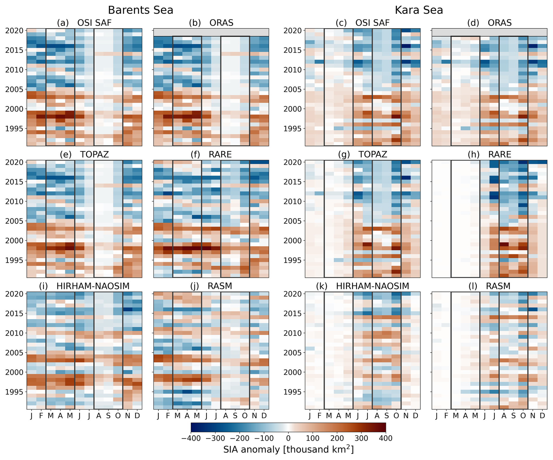
Figure 2 SIA anomaly (SIAa) in each dataset for the Barents (left) and Kara Sea (right). Spring and autumn seasons are marked with dark grey boxes. The anomaly is calculated by taking the difference from the monthly multiyear mean for each month.

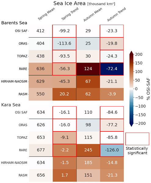
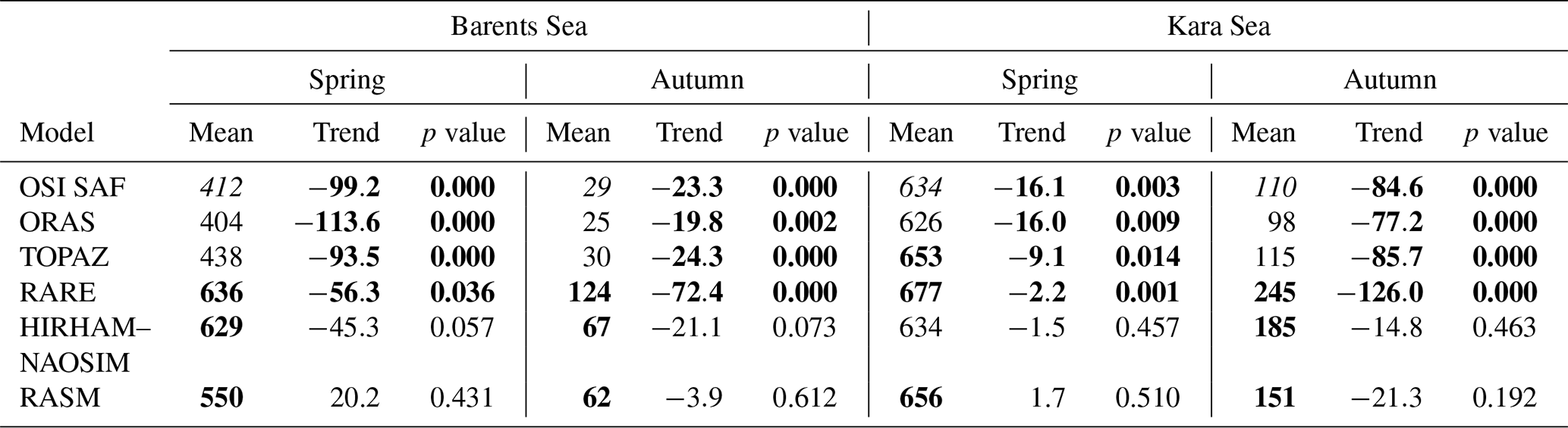
Table 2 Spring and autumn mean SIA [thousand km²], decadal SIA trend [thousand km² decade⁻¹], and p value for Barents and Kara Seas. The values are calculated using the time periods shown in Table 1. Mean values are bold when the yearly seasonal means differ significantly from OSI SAF (t test, p<0.05). Trends and p values are bold when the given p<0.05 (least-squares regression). The full areas used for the comparisions are 1 255 000 km² for the Barents Sea and 682 000 km² for the Kara Sea (Fig. 1).

4.1.1 Barents Sea sea ice area

In the Barents Sea, the satellite observations from OSI SAF indicate a mean SIA of 412 000 km² in spring and 29 000 km² in autumn. According to the observations, the SIA shows statistically significant decadal trends in both seasons during the period 1991–2020 (Table 2). All reanalyses also show a statistically significant SIA trend in both seasons, while the coupled regional models do not. The monthly SIA anomalies (SIAa) for OSI SAF (Fig. 2a) show a similar pattern for each month, indicating that a trend is present throughout the year. In general, the SIA is larger than the multiyear mean before 2006, while smaller SIA values in comparison to the multiyear mean can be seen after 2005. The drop below the climatological mean coincides with winter 2005–2006, when the second-lowest April sea ice extent in the Barents Sea to date was recorded (Fig. 2a). In 2005 and 2006, the maximum SIA of the Arctic had two consecutive record-low years, with persistent negative anomalies in the eastern Arctic basin (Comiso, 2006; Li et al., 2022). Regarding winter extreme SIA, the minimum April extent in 2016 is shown as dark blue between February and May. In contrast, distinctly high winter values occurred in 1998 and 2003.

From the ocean reanalyses, ORAS underestimates the mean area in both spring and autumn, while TOPAZ overestimates it. However, the differences are small and not statistically significant (Table 2). In the spring, ORAS slightly overestimates the trend and TOPAZ slightly underestimates the trend, while the opposite is true in the autumn. ORAS and TOPAZ exhibit temporal variability consistent with OSI SAF, including similar interannual and year-to-year variations (Figs. 2a, b, e and A1).

The ocean reanalysis RARE shows a temporal pattern rather similar to OSI SAF (Fig. 2a and f), with, for example, consistent high and low SIA years. The RARE SIA is, however, overestimated compared to OSI SAF, especially in the autumn (Table 2). RARE also has the largest statistically significant decadal trend in autumn. This greater absolute ice loss occurs from a more extensive mean ice cover. The trend in spring, however, is smaller than that of the other ocean reanalyses and OSI SAF. Thus, RARE reproduces the direction and broad temporal variability of the observed change, but performs less well in representing the mean SIA and the seasonal magnitude of the trend than the other reanalyses. The closer agreement of ORAS and TOPAZ with OSI SAF is expected as both products assimilate satellite-derived sea-ice observations, which constrain their sea-ice state toward observations, whereas RARE does not directly assimilate satellite SIC. This difference likely contributes to the better representation of mean SIA in ORAS and TOPAZ, although sea-ice performance also depends on the assimilation method, atmospheric forcing, and underlying ocean–sea-ice model (Uotila et al., 2019; Storto et al., 2019; Zhang et al., 2021; Xiong et al., 2025). Thus, ORAS and TOPAZ are more suitable for reproducing the observed historical SIA, but their closer agreement with OSI SAF does not necessarily indicate a better representation of the physical processes governing sea-ice variability.

From the coupled regional models, the mean HIRHAM–NAOSIM spring SIA in the Barents Sea is overestimated compared to OSI SAF and closer to that of RARE, and both spring and autumn mean areas are significantly higher than those of OSI SAF, though the SIA in autumn is only about half that of RARE (Table 2). The linear trends for HIRHAM–NAOSIM have p values between 0.05 and 0.1 and are thus not statistically significant. In spring, the trend is smaller than for any reanalysis, while in autumn the trend is close to that of OSI SAF. The negative anomalies are in the majority during the last ten years, signifying an interannual decline (Fig. 2i). In contrast to the three ocean reanalyses and OSI SAF, HIRHAM–NAOSIM has an oscillating SIA with three above-average sea ice periods separated by periods with below-average values (Fig. 2a, b, e, f, and i). RASM spring mean SIA is smaller than that of RARE and HIRHAM–NAOSIM but still statistically different from OSI SAF, while the autumn mean is close to that of HIRHAM–NAOSIM 2). RASM shows no clear trend, only interannual variations (Fig. 2j). The interannual variations in the SIAa for both coupled regional models are similar to each other and closely follow OSI SAF and the reanalyses as well, even though they lack the trend (Figs. 2 and A1a). This suggests that the coupled models reproduce much of the interannual variability in the Barents Sea, but not the magnitude of the observed long-term decline. Of the two coupled models, HIRHAM–NAOSIM performs better in terms of the SIA trend, even though the trend is not statistically significant at p<0.05, whereas RASM has a smaller mean SIA bias. For coupled atmosphere–ocean models, it can not be expected that the results follow observations exactly, as they have their own atmospheric models, reducing the similarity with the ocean reanalyses, which are (directly) forced by the ERA atmospheric reanalysis. The coupled models represent a possible pathway of the climate system rather than a direct reproduction of observed conditions. Although coupled regional models can be driven by quasi-observed data at the lateral boundaries, the simulation inside the model domain evolves freely. Consequently, small differences in the initial state can lead to different simulation results (e.g. Rinke and Dethloff, 2000).

4.1.2 Kara Sea sea ice area

In the Kara Sea, the spring SIA does not statistically differ between OSI SAF, ORAS, and HIRHAM–NAOSIM, while TOPAZ, RASM, and RARE overestimate the mean, but the differences are small (Table 2). In autumn, the mean SIA of ORAS and TOPAZ does not statistically differ from OSI SAF, while RASM, HIRHAM–NAOSIM, and RARE overestimate the mean SIA, with the RARE mean being largest. The differences between the datasets are small in spring because the Kara Sea is typically almost completely ice-covered during this season, limiting the variability of an area-based metric and making SIA relatively insensitive to concentration differences within the compact ice cover (Duan et al., 2019a, b; Kumar et al., 2021). Autumn therefore provides a more discriminating test of model performance in the Kara Sea, because differences in melt, oceanic and atmospheric heat input, and the timing of freeze-up are directly reflected in the position of the ice edge and total ice area.

OSI SAF and the reanalyses show a statistically significant decreasing trend in both seasons (Table 2). In spring, the SIA trend is small, with the TOPAZ trend smaller than OSI SAF and ORAS, and the RARE trend is even smaller. Although the RARE trend is statistically significant, its magnitude is small relative to its mean spring SIA (Table 2) and (Fig. 2c, d, g, and h). In the autumn, however, the RARE trend is larger than in TOPAZ, ORAS, and OSI SAF, of which TOPAZ has the largest trend and ORAS the smallest. Similar to the Barents Sea, the large RARE trend occurs together with an overestimation of the mean autumn SIA, indicating that RARE captures the direction of the observed change but not the mean state of the SIA.

Departures from the climatological mean SIA in the datasets are low in winter and spring (January–April), when the Kara Sea is practically completely ice-covered, even though some SIA anomalies can be seen during this period, being strongest in OSI SAF and ORAS (Fig. 2c and d). The interannual sea ice anomaly patterns in the reanalyses resemble OSI SAF (Fig. 2c, d, g, and h), similarly to what was seen in the Barents Sea. In HIRHAM–NAOSIM, SIA in the Kara Sea is below average in 1992–1995 and decline again below average in 2015, with a clear drop in summer and autumn (Figs. 2k and A1b), even though no statistical linear trend can be seen. RASM does not display any interannual sea ice decline, and its trends are not statistically significant (Table 2 and Fig. 2l). Again, the interannual variation of the coupled regional model resembles that of OSI SAF and the reanalyses, but the difference to OSI SAF is larger than for the Barents Sea (Fig. A1b). Thus, while the coupled models reproduce some of the observed interannual variability, neither reproduces the long-term SIA decline in the Kara Sea.

4.2 Sea ice edge error

Given the good mean SIA agreement of ORAS and TOPAZ with OSI SAF discussed in Sect. 4.1.1, it is not surprising that their integrated ice edge errors (IIEE), relative to OSI SAF, are much smaller than those of the other datasets (Table 3). Furthermore, the monthly mean IIEEs for these products show only small variations (Fig. A2), both in the Barents Sea and in the Kara Sea. In the Barents Sea, TOPAZ has a higher IIEE from January to June due to a greater underestimation of the ice edge location than ORAS (Fig. A2a and c). In the Kara Sea, the largest difference between ORAS and TOPAZ occurs in October and November when TOPAZ overestimates the edge while ORAS underestimates it. The ice edge of TOPAZ tends to recede too fast in early summer and refreeze too fast in early winter, which is most likely the reason for this difference (Bertino and Xie, 2025). The trend of the annual mean O–U is small for ORAS and TOPAZ and decreases over time, indicating increasing accuracy in their ice edge simulation (Table 3 and Fig. A2e). This is consistent with the good agreement in SIA shown in Sect. 4.1. Thus, both products perform well not only in representing the total amount of sea ice, but also its spatial extent.

Table 3 IIEE mean and ice edge Overestimation–Underestimation (O–U) mean, trend, and p value for Barents and Kara Sea. Means and trends are expressed in thousand km². Trends and p values are bold when p<0.05, indicating a significant trend. The trends are calculated from the time series shown in Fig. A2e and f. For the Kara Sea, only the May–December period is analyzed due to the region being fully ice covered in the winter.

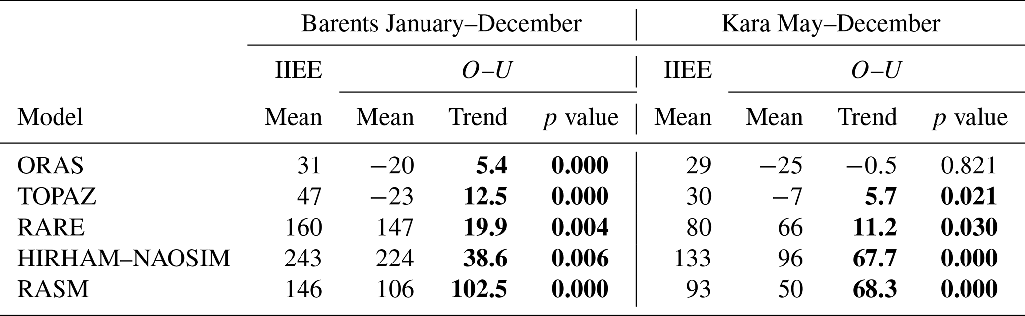
The IIEE of RASM and RARE are similar to each other, with the maximum IIEE in the summer (June or July) (Fig. A2a and b). RARE has a larger mean IIEE in the Barents Sea and RASM a larger one in the Kara Sea (Table 3). The O–U is larger in RARE than in RASM for both regions. The main difference between RARE and RASM is in the O–U trend (Table 3 and Fig. A2e and f). The trend is over 5 times larger in RASM than in RARE, because the ice edge in RASM does not change much over the study period (Sect. 4.3), which results in the model underestimating the ice edge at the start of the study period and significantly overestimating it at the end. Although RARE and RASM have similar mean IIEE values, their behaviour differs substantially. RARE captures the observed decrease in SIA (Sect. 4.1), while the larger O–U trend in RASM reflects its lack of a comparable long-term change.

HIRHAM–NAOSIM has the highest mean IIEE and the highest mean O–U (Table 3). The error is largest in December in the Barents Sea and in October in the Kara Sea (Fig. A2a and b). In the Barents Sea, the trend is smaller than the RASM trend, but in the Kara Sea the trend is similar. The variability from year to year in HIRHAM–NAOSIM is larger than in the other models (Fig. A2e and f). The IIEE results show that a realistic SIA does not necessarily imply a realistic ice edge. For example, RARE reproduces the observed SIA trends better than RASM, while HIRHAM–NAOSIM has a smaller SIA bias than RARE but a larger ice edge error. Evaluating both metrics therefore provides a more complete assessment of model performance.

4.3 Sea ice concentration

The SIC difference between the analysed products and OSI SAF is shown in Fig. 3 for the spring and autumn. The mean SIC and the decadal trends for these two seasons are shown in Figs. 4 and 5. The evolution of the SIC over the study period 1991–2020, along with the differences between the reanalysis and model products against the observed OSI SAF concentration, is discussed in Sects. 4.3.1 and 4.3.2.

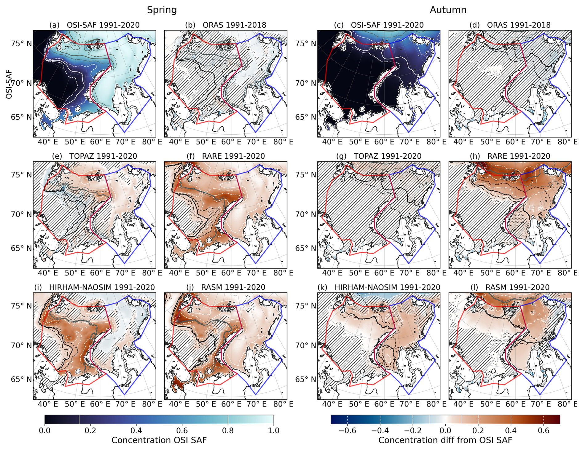
Figure 3 Mean difference between model or reanalysis and OSI SAF SIC for spring (left) and autumn (right), and mean OSI SAF concentration (a, c). The difference plots (b, d–l) have been masked where the difference is not statistically significant (t test, “////” where p>0.1 and “…” where $\mathrm{0.05}<p<\mathrm{0.1}$). The black (white) solid contour lines show the mean ice edge (SIC=15 %), and the grey contour shows the inner boundary of the marginal ice zone (MIZ) (SIC=80 %) for the whole time period. To represent the sea ice edge at the start and the end of the time-series, the dash-dotted lines show the 1991–2000, and the dashed lines the mean from 2011–2020, (2011–2018 for ORAS) for the sea ice edge and the inner MIZ boundary.

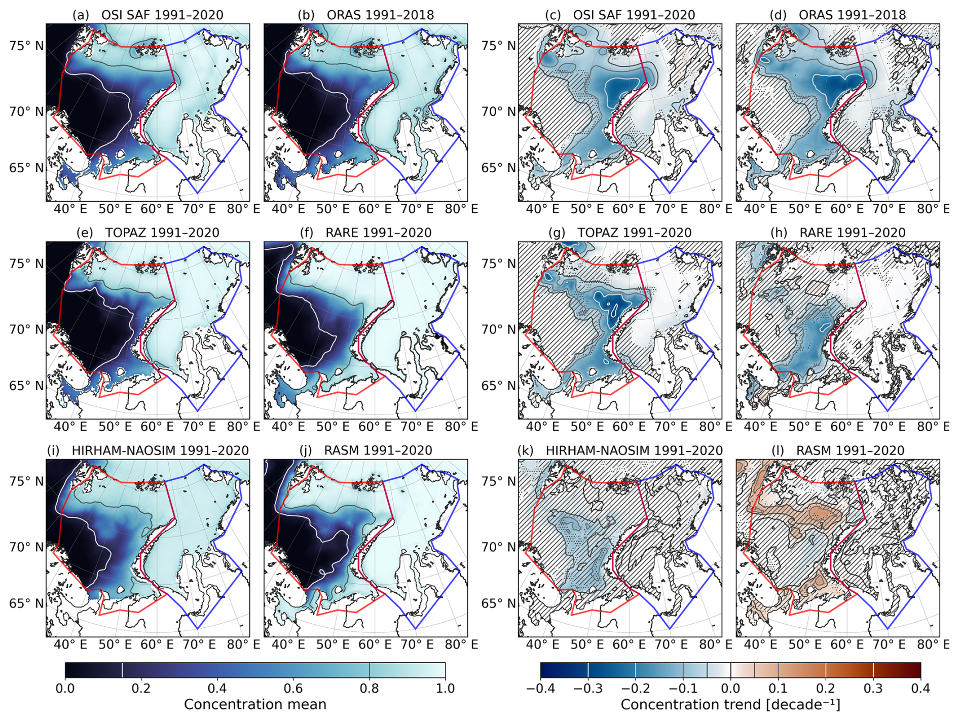
Figure 4 Average SIC mean (left) and trend (right) of all the datasets in spring over the whole period, presented as the fraction of sea ice cover per grid cell. The mean isolines (15 % and 80 % ice concentration) are used to distinguish the MIZ. In the trend subplots, the not statistically significant areas have been masked (“////” where p>0.1 and “…” where $\mathrm{0.05}<p<\mathrm{0.1}$).

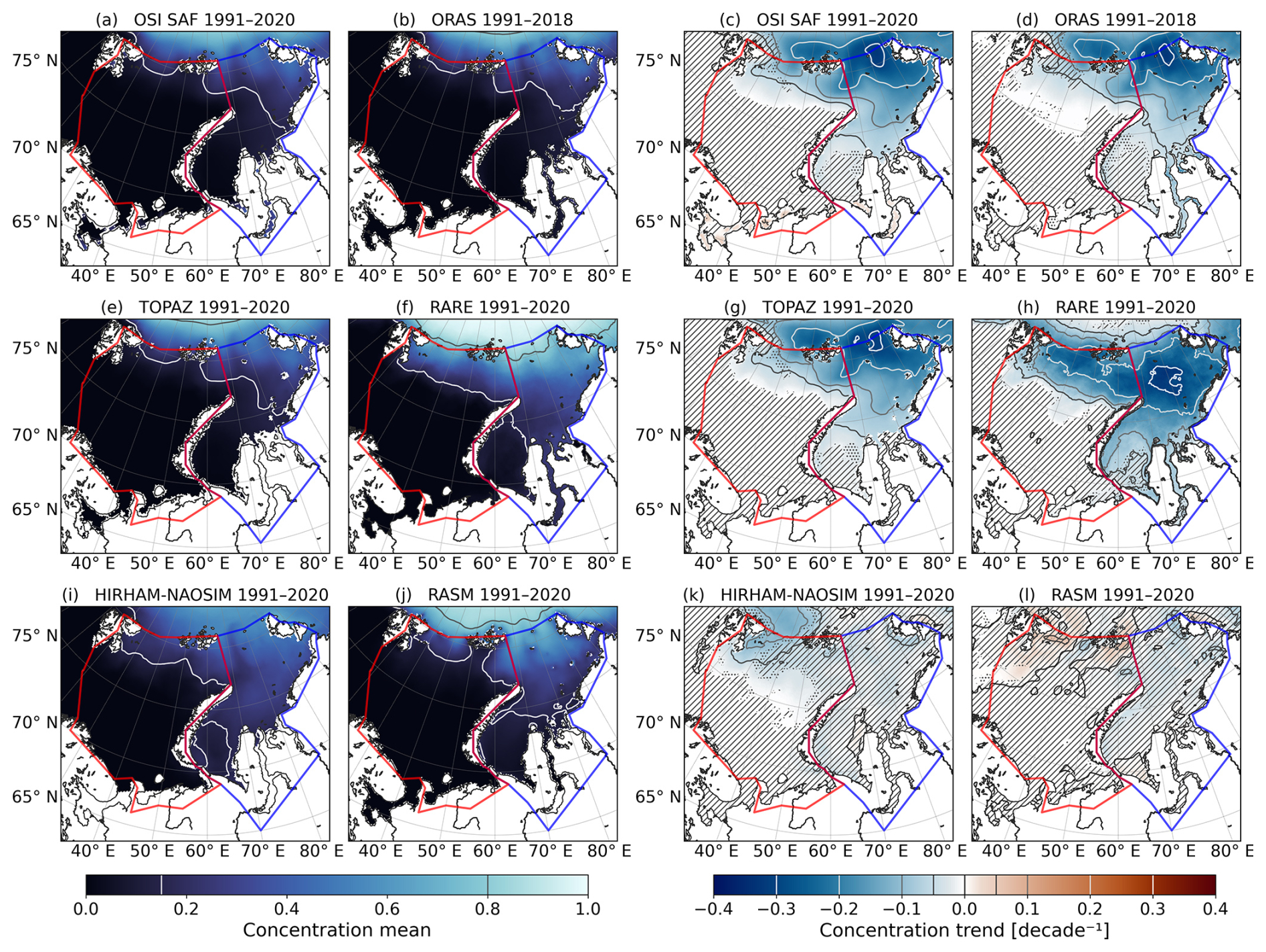
Figure 5 Average SIC mean (left) and trend (right) of all the datasets in autumn over the whole period, presented as the fraction of sea ice cover per grid cell. The mean isolines (15 % and 80 % ice concentration) are used to distinguish the MIZ. In the trend subplots, the not statistically significant areas have been masked (“////” where p>0.1 and “…” where $\mathrm{0.05}<p<\mathrm{0.1}$).

4.3.1 Spring sea ice concentration

In spring, the OSI SAF 1991–2020 mean sea ice edge (SIC=15 %) is located at, or slightly north of, the 75° N latitude until about 50° E longitude, where it turns south-west toward the southern part of the Kola Peninsula (Figs. 3n and 4a). The boundary between the pack ice and the marginal ice zone (MIZ) (SIC=80 %, later called the inner MIZ boundary) goes from south-east Svalbard to the middle of the Barents Sea Exit (BSX) at the Barents and Kara Sea border between Novaya Zemlya and Franz Josef Land (see Fig. 1). Then it turns south towards northern Novaya Zemlya at around 70° E. Another small area with SIC<80 % exists west of Franz Josef Land. In the south, the inner MIZ boundary is located on average at the Kara Gate.

During the first decade, in 1991–2000, the OSI SAF sea ice edge is somewhat southwest and the inner MIZ boundary between Svalbard and Novaya Zemlya is south of the one described above (Fig. 3a). In 2011–2020, the largest retreat of the OSI SAF sea ice edge occurs east of 45° E and is northward and eastward. The ice edge reaches Novaya Zemlya at around 75° N and then extends from southern Novaya Zemlya to the southern Kola Peninsula (Fig. 3a). During this period, the SIC in the Barents Sea is generally below 80 %, except in some small areas in the north-east and north-west; the inner MIZ boundary has retreated at the BSX and the Kara Gate compared to earlier decades. Moreover, there is now a small MIZ area north of the Yenisey Gulf.

The OSI SAF SIC shows statistically significant negative trends for the period 1991–2020 across most of the Barents Sea ice-covered region in spring (Fig. 4c). The negative trend is largest north-west of Novaya Zemlya, close to the region where the sea ice edge retreats at the end of the time series, where the negative trend is larger than 0.2 decade⁻¹. In the Kara Sea, the negative OSI SAF SIC trends are smaller than in the Barents Sea, below $\pm \mathrm{0.05}{\mathrm{decade}}^{-\mathrm{1}}$ and not always statistically significant. An exception to this is at the BSX, Kara Gate, and north of the Yenisei Gulf, where the trends are slightly larger, with a negative trend above 0.1 decade⁻¹ at the BSX.

ORAS is the dataset with a SIC closest to OSI SAF, with no large statistically significant differences in the study area (Fig. 3b). TOPAZ overestimates SIC in the northern Barents Sea and in the Kara Sea. This results in a narrower MIZ than in OSI SAF and in a correspondingly extensive pack ice area in TOPAZ in spring (Fig. 3e). The statistically significant overestimation tends to be larger in the Northern Barents Sea than in the Kara Sea, but is mostly less than 0.1 decade⁻¹ except at the northern edge of the Barents Sea and north of Novaya Zemlya at the BSX (Fig. 3e). TOPAZ SIC trends form a similar spatial pattern to OSI SAF (compare Fig. 4c and g), but with a stronger maximum negative trend west of Novaya Zemlya. In the northernmost part of the Barents Sea, however, the TOPAZ SIC trend is not significant and is smaller than OSI SAF and ORAS and the area with a negative trend above 0.1 decade⁻¹ does not extend into the Kara Sea. Overall, ORAS and TOPAZ reproduce the observed spring SIC and its spatial trend pattern well, although TOPAZ overestimates SIC and has a narrower MIZ indicating a sharper transition between compact ice and open water than in OSI SAF. Although both ORAS and TOPAZ assimilate satellite-derived sea-ice information, they employ different ocean and sea-ice models, vertical coordinate systems, and assimilation approaches. The opposite SIC biases therefore suggest that differences in model physics, sea-ice thermodynamics, ice–ocean coupling, and the implementation of assimilation are at least as important as the assimilated observations themselves. This may be related to the too-rapid seasonal retreat and early refreezing discussed in Sect. 4.2.

RARE overestimates SIC relative to OSI SAF in spring over most of the sea ice covered area (Fig. 3f). The ice edge and the inner MIZ boundary are too extensive, being further south and east than the OSI SAF boundary. The RARE SIC is more than 0.1 above OSI SAF in the southern Kara Sea, in the Kara Sea at the BSX, and in most of the ice-covered Barents Sea. The difference is above 0.4 south of Svalbard and west of Novaya Zemlya. The RARE ice edge in spring retreated eastward and northward between 1991–2000 and 2011–2020 (Fig. 3f), while the inner MIZ boundary changed wery little. The RARE SIC has a negative trend in the Barents Sea south of 75° N that is mostly below 0.2 decade⁻¹, but no meaningful significant trend north of that or in the Kara Sea. (Fig. 4h). Thus, RARE captures part of the observed spring SIC decline in the southern Barents Sea, but overestimates SIC and shows little change farther north and in the Kara Sea. This is consistent with its SIA and ice-edge overestimations in Sects. 4.1 and 4.2 and may partly reflect that RARE constrains sea ice indirectly through a PIOMAS-based surface heat-flux relaxation rather than directly assimilating satellite SIC (Carton and Chepurin, 2023). In addition, the PIOMAS data used for the sea ice constraint have a coarser spatial resolution than the satellite observations assimilated in TOPAZ and ORAS, which may further contribute to the larger discrepancies between RARE and OSI SAF.

Similar to RARE, the RASM SIC is also significantly overestimated for most of the region, but with an area where the difference is not statistically significant in the middle to northern part of the Barents Sea between 40 and 60° E (Fig. 3j). RASM is the model with the largest concentration differences, with even above 0.6 decade⁻¹ differences south of Svalbard and on the west coast of Novaya Zemlya. The sea ice edge only retreats in a small area west of Novaya Zemlya, and the changes to the inner MIZ boundary are small. The SIC is statistically significant in small areas close to the inner MIZ boundary in the Barents Sea, where the trend is positive, with some small regions with a positive trend above 0.1 decade⁻¹ (Fig. 4j and l). The absence of widespread negative SIC trends despite the observed decline indicates that RASM fails to reproduce the long-term reduction of sea ice. This is consistent with the lack of a significant SIA trend discussed in Sect. 4.1.

The HIRHAM–NAOSIM spring SIC difference from OSI SAF (Fig. 3i) differs from the other datasets in that it is underestimated in the north and western half of the Kara Sea and overestimated in the southeastern Kara Sea and in most of the ice-covered Barents Sea. The ice edge is located too far southwest compared to OSI SAF (Fig. 3a and i), while the inner MIZ boundary does not extend east of 60° N. The ice edge retreats, but not as much as for OSI SAF, and the negative SIC trend is only statistically significant in small parts of the MIZ in the Barents Sea and at the north-eastern coast in the Kara Sea (Figs. 3i and 4k). Of the coupled models, HIRHAM–NAOSIM reproduces the observed spring SIC decline best, but only in the Barents Sea and with significant decreasing trends only present in parts of the MIZ. This indicates that the model underestimates the spatial extent of the ongoing sea ice retreat

4.3.2 Autumn sea ice concentration

In autumn, the OSI SAF SIC is above 15 % in the northern part of the study area (Fig. 3c). The mean sea ice edge goes from north of Svalbard to Franz Josef Land, from Franz Josef Land to the middle of the BSX, then continues eastward, and finally turns southward at around 80° E (Figs. 3c and 5a). OSI SAF shows significant negative trends in the whole ice-covered area (Fig. 5a). In 1991–2000, the sea ice edge goes from Svalbard to the northern tip of Novaya Zemlya and then from the north-east of Novaya Zemlya to the Yamal Peninsula. In comparison, the 2011–2020 mean sea ice edge goes north of the Barents Sea and along the northern boundary of the Kara Sea (Fig. 3c).

Autumn SIC of TOPAZ and ORAS do not differ significantly from OSI SAF (Fig. 3d and g), and the ORAS and TOPAZ decadal trends are almost identical to those of OSI SAF (Fig. 5d and g). Compared to OSI SAF, RARE overestimates the autumn sea ice edge and concentration, with the largest differences in the northern part of the study region (Fig. 3h). For autumn, RARE is the dataset with the largest concentration overestimation. The RARE mean sea ice edge goes from southern Svalbard to the northern tip of Novaya Zemlya, then continuing to the Yamal Peninsula (Figs. 3h or 5i). As for OSI SAF, the RARE negative trend in SIC extends over the sea ice covered area (Fig. 5h), but the maximum trend is stronger and located farther south than in OSI SAF. This can partly be explained by RARE retaining sea ice in areas where OSI SAF, ORAS, and TOPAZ become ice-free, leaving more ice available to decline.

The HIRHAM–NAOSIM sea ice edge in the Barents Sea goes from southern Svalbard to northern Novaya Zemlya, similar to RARE, but in the Kara Sea the edge is even further south (Fig. 3k). Most of the ice covered area has an overestimated SIC, except in the northernmost part where the differences compared to OSI SAF are not statistically significant. The overestimations are, however, clearly less than for RARE. The negative SIC trend in HIRHAM–NAOSIM is statistically significant and above 0.05 decade⁻¹ only in a small region east of Svalbard (Fig. 5k).

The RASM mean autumn sea ice edge is further north than the HIRHAM–NAOSIM and RARE sea ice edge, and the SIC is overestimated less than in RARE but more than in HIRHAM–NAOSIM, with overestimation above 0.2 decade⁻¹ in the northern parts (Fig. 3l). However, the SIC is not statistically significantly different from OSI SAF in the eastern Kara Sea at the coast. RASM does not have any meaningful significant trend in the SIC in autumn (Fig. 5l). Unlike in spring, where HIRHAM–NAOSIM reproduces part of the observed decline in the Barents Sea MIZ, neither coupled model reproduces the widespread autumn SIC decline. HIRHAM–NAOSIM performs somewhat better by showing a small area of significant decline east of Svalbard, whereas RASM shows no meaningful autumn trend. Together with their overestimated SIC, this indicates that the seasonal sea ice retreat is too weak in both models, particularly in the Kara Sea.

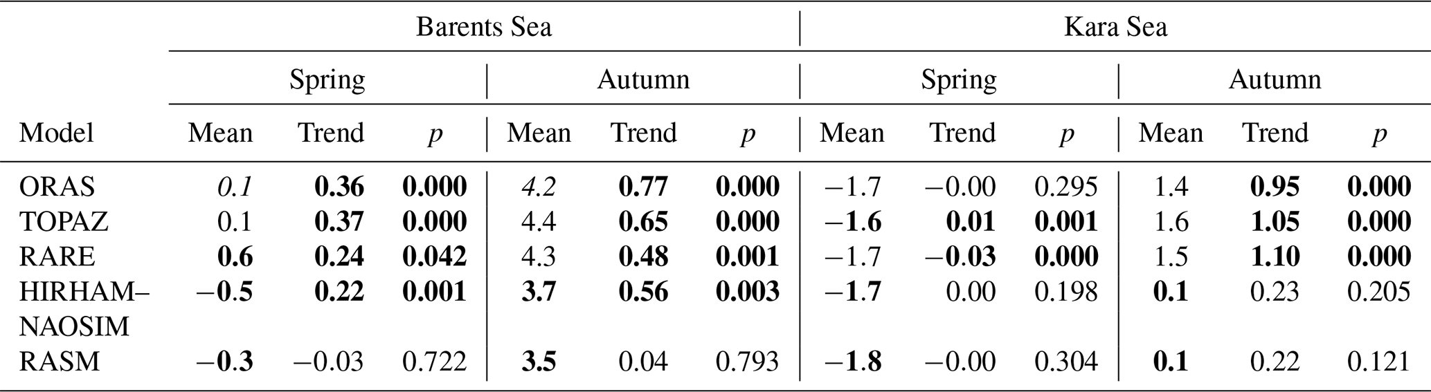
Table 4 Spring and autumn mean ML temperature [°C], decadal trends [°C decade⁻¹], and p values for Barents and Kara Seas. Calculated for the maximum period of each dataset. Mean values are bold when the seasonal means differ significantly from ORAS5 (t test, p<0.05, 1991–2018). Trends and p values are bold when the given p<0.05 (least-squares regression).

4.4 Ocean temperature of the mixed layer

The mean temperature and trends of the ML are shown in Table 4 for spring and autumn. In the Barents Sea, the spring mean temperature varies from −0.5 °C (HIRHAM–NAOSIM) to 0.6 °C (RARE) between the models. RARE is considerably warmer than ORAS and TOPAZ, while HIRHAM–NAOSIM and RASM are colder. The mean ML temperature in the regions stays mostly below 5 °C, except in RARE, where some warmer waters can be seen (Fig. A3d). For the other models, the difference in the regional mean seems to depend more on how widespread the warmer waters are than the difference in temperature of the warmer waters (compare Fig. A3a, c–g, and h). In the Kara Sea, the spring variation is smaller and the ML is close to freezing (Table 4). In autumn, the mean ML temperature does not significantly differ between the reanalyses in either the Barents or the Kara Sea, while both models are significantly colder (Table 4). The mean ML temperature stays mostly below 10 °C in the Barents Sea, except in the south-west in RASM (Fig. A4) and mostly below 5 °C in the Kara Sea, except in the south-west in RASM, RARE, and TOPAZ (Fig. A4c, d, and h). The reason why the regional mean for HIRHAM–NAOSIM and RASM is similar, even if RASM has these warmer coastal waters, is that many of these are outside of the compared region (Fig. 1). The colder mean mixed-layer temperatures in the coupled models relative to the reanalyses, particularly in autumn, are consistent with their tendency to maintain too much sea ice (Sects. 4.1 and 4.3). A more extensive ice cover reduces the direct exposure of the ocean to atmospheric forcing and can limit seasonal ocean warming, suggesting that at least part of the temperature bias may be linked to the sea-ice bias rather than to ocean processes alone.

The ML temperature trend is positive and statistically significant in the Barents Sea in both spring and autumn for the reanalyses and for HIRHAM–NAOSIM, being stronger in the autumn (Table 4). In spring, the warming trend in HIRHAM–NAOSIM, ORAS, and TOPAZ is highest in the ice-free areas or close to the ice edge (Fig. A3b, e, and i), while in the autumn ORAS and TOPAZ have a significant warming trend over the whole Barents Sea. The warming trend is weaker and the region of significant warming is smaller in HIRHAM–NAOSIM and does not extend as far north and east. In RARE, the highest spring warming coincides with deeper areas (Fig. 1), where Atlantic water enters the Barents Sea (Skagseth et al., 2008). This partly coincides with the area of the strongest decreasing SIC trend in the MIZ east of Novaya Zemlya (Figs. 4j and A3k). The trend in spring at these locations is stronger than in ORAS, and the two areas are separated by a nonsignificant cooling trend. In autumn, RARE has two areas with a cooling trend, of which the eastern one at the coast of Novaya Zemlya is statistically significant. These are located close to the same areas where there was the strong warming trend in the spring. The ML temperature in this location is also on average warmer than in the other reanalyses (Fig. A3d and f). Of these, the eastern one is located west of Novaya Zemlya, in the same location as the strong warming in spring and is statistically significant. In autumn, RARE also shows a statistically significant deepening of the ML west of Novaya Zemlya (not shown). The contrasting spring warming and autumn cooling in this region may indicate differences in how vertical mixing and the seasonal storage and release of ocean heat are represented in RARE compared to the other reanalyses. The present analysis cannot isolate the respective contributions of the ocean model, assimilation scheme, and atmospheric forcing to this behaviour.

In the Kara Sea, the trend is small for all datasets in spring, when the region is ice-covered (Table 4). The limited spring warming is therefore consistent with the weak spring SIA and SIC trends, because the compact ice cover (SIC>80 %) restricts atmosphere–ocean heat exchange and keeps the ML temperature close to freezing. In autumn, the trend is statistically significant in the reanalyses and close to 1 °C decade⁻¹ (Table 4). The autumn ML temperature trend is above 1 °C decade⁻¹ in large areas of the Kara Sea in all reanalyses and is stronger in the Kara Sea than in the Barents Sea. HIRHAM–NAOSIM shows no statistically significant trend in the Kara Sea where the sea ice is overestimated (Sect. 4.3.2 and Fig. 5i). RASM has no widespread statistically significant trends in either region in spring or autumn, only small areas of warming in the Kara Sea and cooling in the Barents Sea (Fig. A4i and j). Thus, HIRHAM–NAOSIM reproduces the Barents Sea warming better than RASM, but neither coupled model captures the pronounced autumn warming in the Kara Sea. For HIRHAM–NAOSIM, the weak Kara Sea warming coincides with its extensive sea-ice cover, which may limit seasonal atmosphere–ocean heat exchange. RASM, by contrast, shows weak ML temperature trends despite a less extensive sea-ice bias, suggesting that its lack of warming cannot be attributed to excessive ice cover alone.

Table 5 Pearson's correlation coefficients between SIA and ML temperature of Barents and Kara Sea, denoted as r, and between the SIAa (Fig. 2) and ML temperature anomaly (MLTa) (Fig. A5), denoted as r_diff. For r_diff, bold numbers are statistically significantly different from ORAS r_diff using Fisher's z test (p<0.05), while italic shows where Barents and Kara Sea differ from each other.

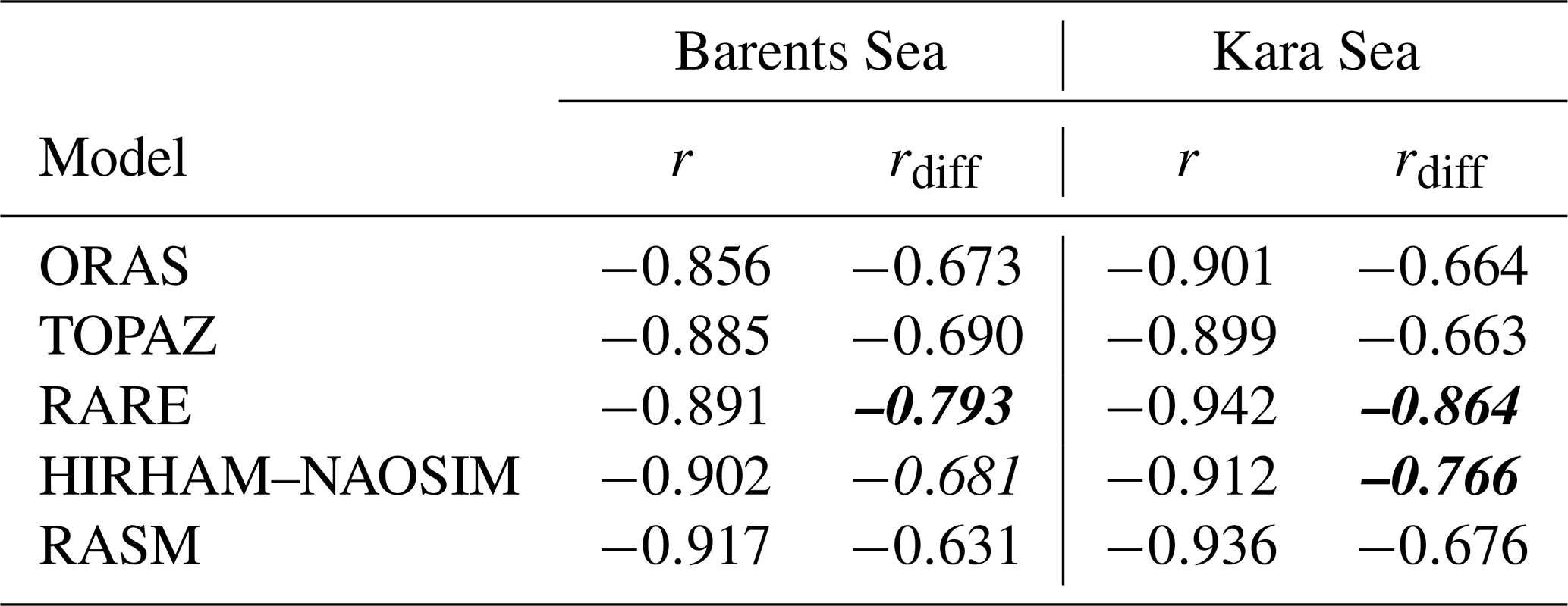
Table 5 shows the PCC calculated between SIA and ML temperature and between the anomalies (shown in Figs. 2 and A5). The average ML temperature anomalies (MLTa) (Fig. A5) follows similar patterns to that of the SIA (Fig. 2), discussed in Sects. 4.1.1 and 4.1.2, though in the Kara Sea, the year-to-year variations are only seen in summer and autumn (for all models). The PCC (r) (Table 5) between the sea ice and temperature is negative for all datasets and ranges between −0.85 and −0.94. The PCC between the anomalies (r_diff), where the effect of the annual variation is removed, is also negative and ranges between −0.63 and −0.86. These high correlations are in line with previous studies (Kumar et al., 2021; Li et al., 2022). The consistently strong negative correlations indicate that all datasets capture the expected tight coupling between mixed-layer temperature and sea ice, whereby warmer upper-ocean conditions favour sea-ice loss and reduced ice cover enhances ocean heat uptake. RARE seems to have a higher correlation between the anomalies than the other datasets and is significantly higher than ORAS in both the Barents Sea and the Kara Sea. In the Barents Sea, only the RARE anomaly PCC (r_diff) differs significantly from ORAS, while in the Kara Sea the difference compared to ORAS is statistically significant for RARE and HIRHAM–NAOSIM. The correlation coefficients between the anomalies are slightly lower in the Kara Sea than in the Barents Sea for ORAS and TOPAZ and slightly higher for the other datasets. However, the differences are statistically significant (Fisher's z test, p<0.05) only for RARE and HIRHAM–NAOSIM. The stronger coupling in RARE may indicate that sea-ice variability is more tightly linked to local ML temperature variability than in the other products. One possible explanation is that RARE constrains sea ice indirectly through surface heat flux relaxation based on PIOMAS (Sect. 2.2; Carton and Chepurin, 2023). This interpretation is consistent with the product-specific spatial temperature behaviour described above, although the present results do not identify the mechanism responsible for the stronger correlation.

4.5 Climate index correlation

PCC of five climate indices (Sect. 3.3) to SIAa and average MLTa were calculated for both regions to explore the teleconnections in the data (Fig. 6). Maps for the correlation of the climate indices per gridcell to the SIC anomaly (SICa) and MLTa, from which the SIAa and average MLTa have been calculated, can be found in the appendix (Figs. A6–A10). Overall, none of the climate-index correlations differ significantly among OSI SAF, ORAS, and TOPAZ for SIAa, or between ORAS and TOPAZ for MLTa. This agreement is expected given the small differences among these datasets found in the preceding sections.

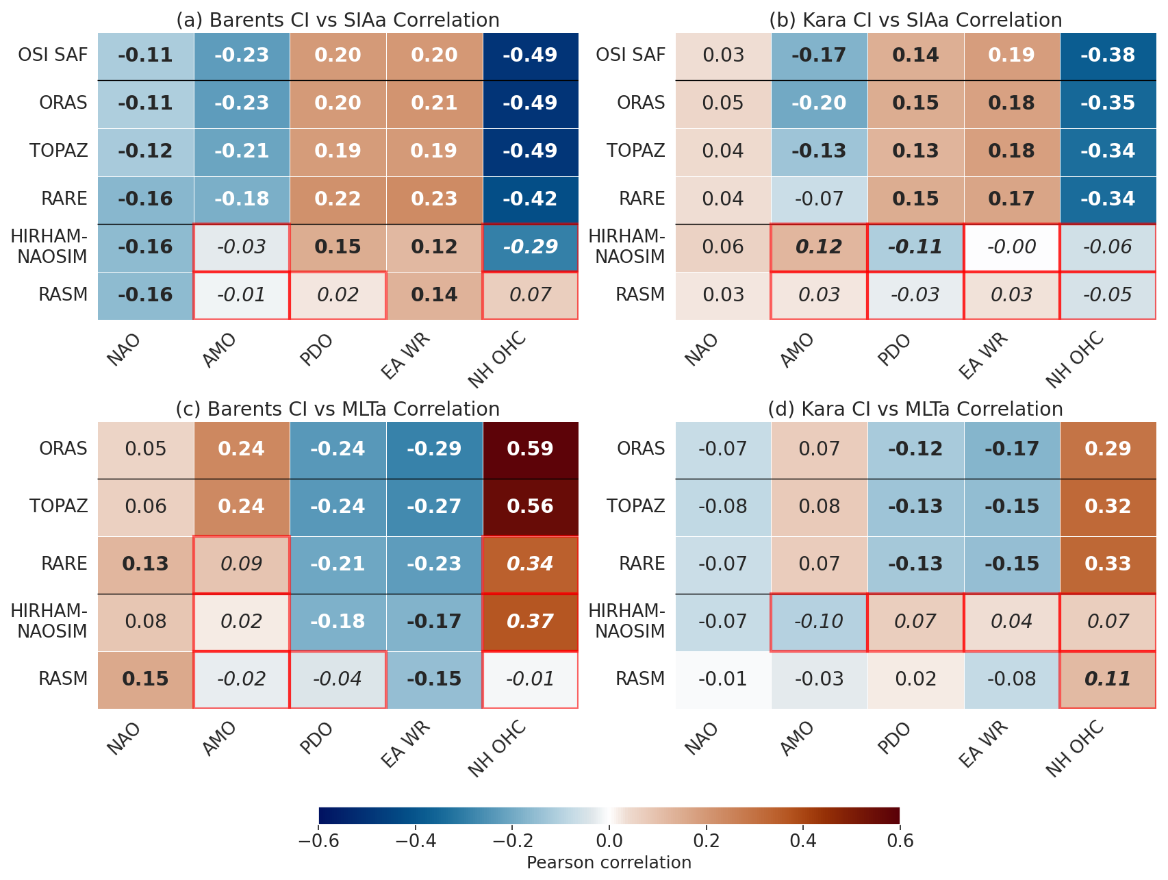
Figure 6 Correlation between climate indices and SIAa (a, b) and average MLTa (c, d) for the Barents and Kara Seas. Correlation values in bold indicate that the correlation is statistically significant (p<0.05), and the red squares indicate where the correlations are statistically different (Fisher's z test, p<0.05) from OSI SAF for SIA and ORAS for MLT. NAO: North Atlantic Oscillation; AMO: Atlantic Multidecadal Oscillation; PDO: Pacific Decadal Oscillation; EA/WR: East Atlantic/Western Russia teleconnection; NH OHC: Northern Hemisphere Ocean Heat Content (0–700 m).

For NAO, there are no significant differences between the datasets (Fig. 6). The positive NAO phase is characterised by a stronger North Atlantic pressure gradient and enhanced westerly circulation, whereas the negative phase is associated with a weaker pressure gradient and weaker or more meridional circulation (NOAA CPC, 2026). A positive NAO leads to warm and humid westerly winds and enhanced heat transport into the Barents Sea region, leading to decreasing sea ice and a statistically significant correlation in SIAa in the Barents Sea (Fig. 6a). The effect is, however, weaker further away from the Atlantic in the Kara Sea, and there the SIAa correlation is not statistically significant (Fig. 6b). The correlation map (Fig. A6a, b, e, f, i, and j) shows that the negative correlation with sea ice is significant mostly in the northern Barents Sea, and a non-significant negative correlation extends into the northeastern Kara Sea. The rest of the Kara Sea is positively correlated but only statistically significant in small areas.

A positive AMO is characterised by warmer-than-average North Atlantic sea-surface temperatures and has been linked to subsequent temperature variability in the Barents Sea (Seip and Wang, 2023), increasing the heat transport to the Barents Sea. Consistent with this relationship, a positive AMO is associated with a negative SIAa and positive MLTa correlation for OSI SAF, ORAS, and TOPAZ, which is about double the correlation with NAO (Fig. 6a and c). In the Kara Sea, we see a weaker, though still significant, correlation in the SIAa, but not in the MLTa as the effect of the Atlantic is again weaker in the Kara Sea (Fig. 6b and d). This difference between SIAa and average MLTa may arise because sea-ice variability integrates the cumulative effects of atmospheric and oceanic forcing, whereas the ML is close to freezing and insulated from the atmosphere during the winter and spring months by the ice cover, dampening the correlation. From the correlation map (Fig. A7a, b, and e) one can see that the negative correlation to SICa is highest for OSI SAF, ORAS, and TOPAZ in the northern Barents Sea. A weaker negative correlation appears in the Kara Sea. A notable feature is an area of positive statistically significant correlation to SICa in the centre of the Barents Sea in OSI SAF, ORAS, and TOPAZ. This could be because currents and winds collects ice here from the surrounding. For MLTa (Fig. A7d and g), ORAS and TOPAZ have a positive correlation for most of the area – strongest in the western Barents Sea and weakest in the Kara Sea, where only small areas are statistically significant. In RARE (Fig. A7f and h), the sea ice correlation is similar but weaker than in the other reanalyses. For MLTa, however, there are some areas with strong negative correlation. These regions coincide with the anomalous ML behaviour identified for RARE in Sect. 4.4, particularly west of Novaya Zemlya (Figs. A3d, f and A4d, f). The negative correlations therefore appear to be associated with the anomalous ML behaviour in RARE, although the underlying cause of this product-specific relationship cannot be determined from the present analysis. For HIRHAM–NAOSIM (Fig. A7i and k), the SICa correlation looks similar to the reanalyses for the western Barents Sea, but is positive for the eastern Barents Sea and for the Kara Sea. The same pattern, although with opposite correlation, can be seen for the MLTa as well. RASM correlations are generally weaker (Fig. A7j and l), with Barents Sea SICa divided into negative correlation in the north and positive in the south, and with Kara Sea showing no large areas of statistically significant correlation.

For PDO, a warm (cold) central northern Pacific is related to a negative (positive) PDO phase. When the central northern Pacific is warm (negative PDO), warm-air advection to the Barents and Kara Seas increases, causing a negative SIAa and positive MLTa. This results in a positive (negative) correlation for the SIAa (MLTa). The PDO correlation is opposite to the AMO correlations and of approximately the same size (Fig. 6). The correlation patterns are similar to those for AMO too (Fig. A8), but with more spread for the SICa correlations in the reanalyses. RARE PDO-MLTa correlation (Fig. A8h) shows an area of positive correlation, but not as large and strong as for the AMO. HIRHAM–NAOSIM PDO correlations (Fig. A8i and k) show a similar east–west divide as for AMO, but the divide is more eastward, resulting in only PDO showing a significantly different correlation (Fig. 6). RASM is significantly different from OSI-SAF and ORAS for both regions (Fig. A8j and l). The correlation for both SICa and MLTa to PDO in RASM is generally non-significant and spatially inconsistent.

The positive (negative) EA-WR produces negative (positive) temperature anomalies over eastern Europe, including the Ural Mountains. As a result, a positive (negative) phase pushes more (less) continental air into the Barents and Kara seas, leading to a generally positive EA-WR – SIA correlation and negative EA-WR – MLTa correlation (Fig. 6), which is seen in all reanalyses and in the Barents Sea also for the coupled models. In the Kara Sea, however, neither coupled regional model has a statistically significant correlation either for SIAa or MLTa. From the map (Fig. A9) we see that the correlations are weaker in the models than in the reanalyses. HIRHAM–NAOSIM has even an opposite, non-significant, correlation in the northeastern Barents Sea and in most of the Kara Seas, while RASM has a non-significant opposite correlation in the northern parts of the study area.

The NH OHC is the climate index that is most affected by the global warming trend and which shows the strongest correlation to both SIAa and MLTa for OSI SAF, ORAS, TOPAZ, and RARE (Fig. 6). It is a good indicator for overall climate warming, as 90 % of the global warming heat is absorbed into the ocean (IPCC, 2021). For OSI SAF, ORAS, and TOPAZ, the correlation with SICa is negative and strongest in the northern Barents Sea, whereas the MLTa correlation is positive and strongest in the western Barents Sea (Fig. A10a, b, d, e, and g). For RARE, the SICa correlation is slightly weaker than for the other reanalyses, but always negative, while in MLTa the biases in the Barents Sea, that was mentioned before in Sect. 4.4 and for AMO and PDO, can again be seen (Fig. A10f and h). The correlations in HIRHAM–NAOSIM in the Barents Sea are in the same direction as in the reanalyses for both SICa and MLTa, but they are weaker and significantly different from those for OSI SAF, ORAS, and TOPAZ (Fig. A10i and k). In the Kara Sea, however, the HIRHAM–NAOSIM does not show a statistically significant correlation. For RASM the only region with a wider statistically significant correlation is the southeastern Kara Sea, where there is a weak correlation to MLTa (Fig. A10l).

For the coupled regional models, HIRHAM–NAOSIM does better in the Barents Sea than RASM for both SIAa and average MLTa correlations. In HIRHAM–NAOSIM, only the AMO and NH OHC correlations differ significantly from OSI SAF (or ORAS in the case of MLTa), while for RASM, AMO, PDO, and NH OHC correlations differ significantly. In the Kara Sea, HIRHAM–NAOSIM SICa (MLTa) correlations with the climate indices differ significantly from OSI SAF (ORAS) for all climate indices except NAO, while RASM SICa climate-index correlations differ significantly for the same indices but do not show the opposite AMO and PDO correlations found in HIRHAM–NAOSIM. For MLTa, only the NH OHC correlation differs significantly in RASM. The differences from observations and reanalyses may partly arise because the coupled regional models simulate interactive atmosphere–ocean–sea-ice processes, whereas the ocean reanalyses are driven by prescribed atmospheric forcing and constrained by assimilated observations. However, the differences between HIRHAM–NAOSIM and RASM also indicate model spread arising from their different components and configurations. The significantly different AMO and NH OHC correlations in both coupled models suggest that the influence of North Atlantic variability is not fully represented. This is consistent with the findings of Yamagami et al. (2022), who showed that Gulf Stream warming contributes to Barents–Kara sea-ice decline and that an underestimation of this warming can lead to an underestimation of sea-ice loss.

A plausible interpretation is that biases in the representation of Atlantic-origin warming affect the ability of the coupled models to reproduce the observed decline in sea ice and increase in mixed-layer temperature. Enhanced warming in the North Atlantic can increase heat transport through the Nordic Seas and Barents Sea, contributing to upper-ocean warming and sea-ice retreat in the Barents–Kara region. The weaker mixed-layer warming trends and weaker sea-ice decline seen in the coupled models are therefore consistent with an under-representation of this mechanism. Although the present analysis cannot determine whether the deficiency originates from the simulation of remote North Atlantic processes, the propagation of heat anomalies into the Arctic, or local ocean–atmosphere–sea-ice feedbacks, the results suggest that Atlantic warming signals are not transmitted to the Barents and Kara Seas.

5 Conclusions

Coupled models and reanalyses were evaluated against OSI SAF satellite measurements regarding their performance in representing the sea ice in the Barents and Kara Seas. The satellite measurements show a significant decreasing trend in the SIA in both seas in both spring and autumn. All three reanalyses reproduce this decline in both seasons, whereas neither coupled regional model reproduces a statistically significant SIA decline in the Kara Sea, and only HIRHAM–NAOSIM shows a near-significant decline in the Barents Sea.

ORAS and TOPAZ show the closest agreement with OSI SAF for sea-ice area, sea-ice concentration, and ice-edge location. RARE, HIRHAM–NAOSIM, and RASM generally overestimate sea ice extent and concentration, resulting in larger ice-edge errors. Among the coupled models, HIRHAM–NAOSIM reproduces aspects of the observed decline better, whereas RASM shows no long-term change in sea ice conditions. The mixed-layer temperature results are consistent with the sea-ice analysis. The reanalyses show significant warming trends, particularly in autumn, whereas the coupled models exhibit substantially weaker warming. In the Kara Sea, significant autumn warming is only reproduced by the reanalyses. Climate index correlations further show that ORAS and TOPAZ reproduce the observed variables most consistently. RARE's problems seem to stem mostly from the anomalous behaviour of the ML temperature discussed in Sects. 4.4 and 4.5. HIRHAM–NAOSIM generally performs better than RASM in the Barents Sea, while both models struggle considerably with the Kara Sea, RASM slightly less. Overall, the reanalyses, particularly ORAS and TOPAZ, provide the most realistic representation of recent sea-ice and mixed-layer temperature variability in the Barents and Kara Seas. The coupled regional models reproduce some aspects of interannual variability but underestimate the observed long-term changes, especially in the Kara Sea.

Overall, ORAS and TOPAZ perform almost equally well in representing the observed sea ice conditions, although ORAS performs slightly better in the spring SIC. Both products are therefore suitable for studies requiring a realistic representation of recent observed climate, while it is still important to take into account their data assimilation if SIC and SST. RARE is also able to produce the trend seen in the satellite observations, but overestimates the sea ice and shows anomalous behaviour in the Barents Sea MLT (Sects. 4.4 and 4.5). We suggest further research and possibly modelling studies into the reasons behind the seen anomalies, whether they result from the ocean model, from the assimilation scheme or from the forcing.

For applications where models and not reanalyses are needed, which of the models we would recommend depends on the use case and the region. These applications include the ones analysing air–sea fluxes, which reanalyses are not able to realistically simulate. RASM has a better mean state of the sea ice, but for any study looking into the changes happening in the Arctic, the total lack of a trend in the Barents Sea is a problem. Therefore, we recommend HIRHAM–NAOSIM over RASM in such cases for the Barents Sea. However, for the Kara Sea, where both models lack the trend, the better mean sea ice representation of RASM might make it the better choice. For HIRHAM–NAOSIM, further research could focus on looking more closely into the behaviour of the model over the Kara Sea and also the eastern part of the Barents Sea. Our research only looked into the first ensemble member of the HIRHAM–NAOSIM model. An interesting question would be whether the lack of a trend, too wide autumn sea ice, and the opposite correlations in the climate indices persist over all the ensemble members. If they do, then a deeper study into the model to find the processes behind the Kara Sea performance is suggested. For RASM, the biggest problems of the model come down to the total lack of trend in the sea ice and ML temperature. More research into the reasons of this could considerably improve the model. For example, the Atlantic Ocean lateral boundary temperature trends might result in sea ice and ML temperature trends in RASM. Future studies could also account for delayed responses to large-scale climate variability through lead-lag analysis and use methods such as multiple regression or machine learning to distinguish the combined and potentially nonlinear effects of the different drivers. Even though the Barents and Kara Seas cover only approximately 11 % of the Arctic Ocean, they have contributed 30 %–40 % of the recent Arctic winter sea ice loss and influence the ocean, sea ice, and atmosphere farther downstream. Improving the representation of these regions in coupled models is therefore important not only for regional studies, but also for understanding Arctic and global climate variability and change.

Appendix A: Additional figures

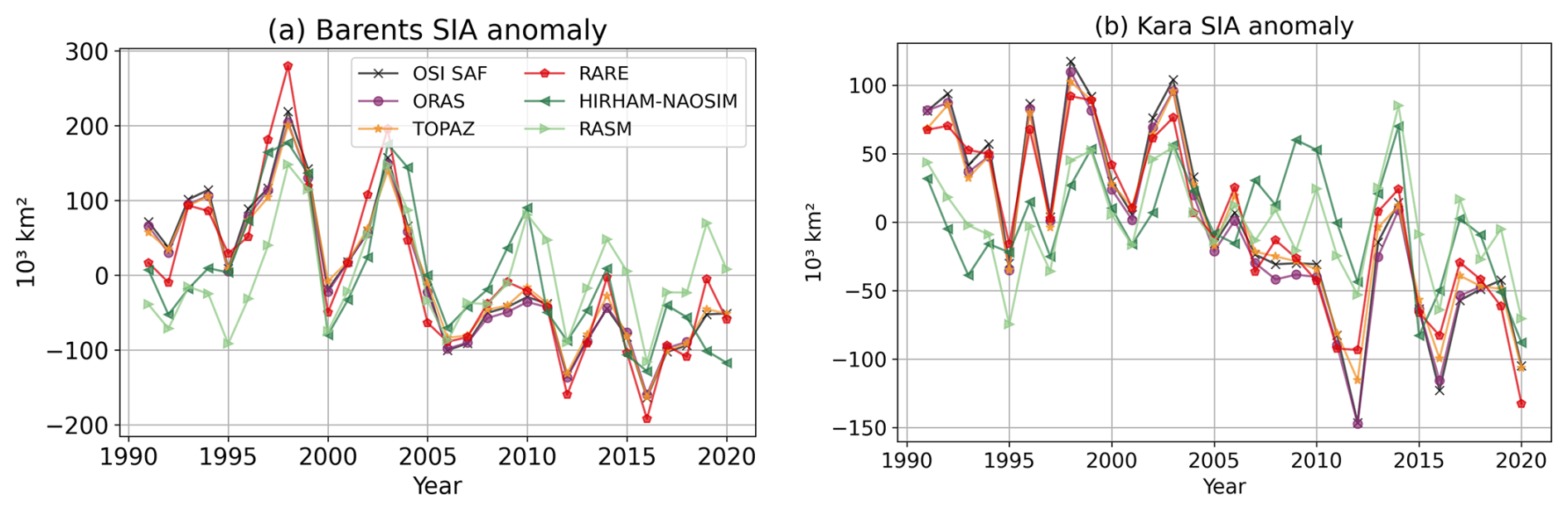
Figure A1 Yearly mean of the monthly SIA anomalies for Barents (a) and Kara Sea (b) in each model shown in Fig. 2.

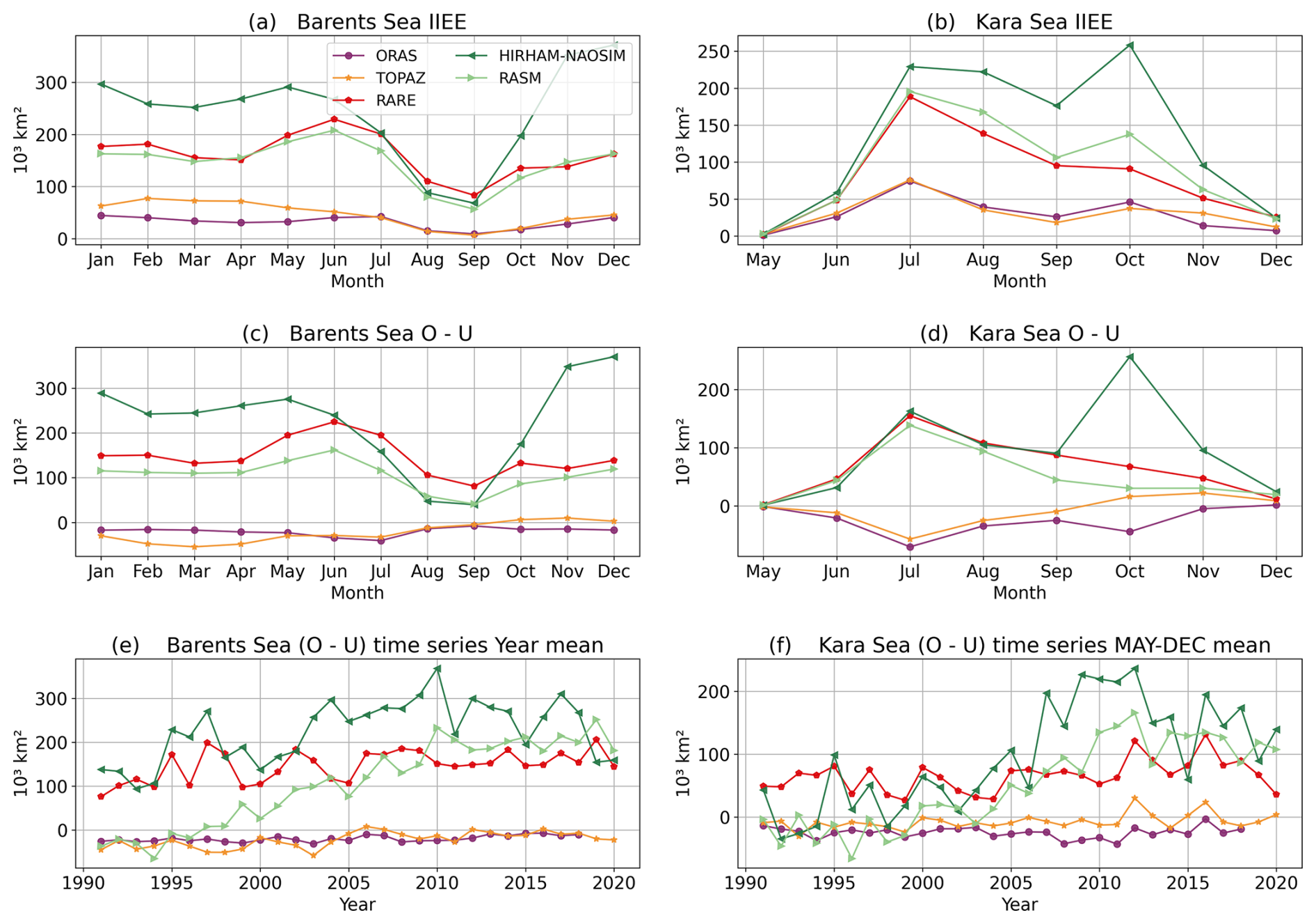
Figure A2 Integrated Ice Edge Error (IIEE) of the (a) Barents and (b) Kara Seas, as well as (c, d) Overestimation–Underestimation of the sea ice edge, and (e, f) time series of the yearly mean Overestimation-Underestimation. For the Kara Sea, only values during May–December are shown, as there is no ice edge during winter and spring in most years.

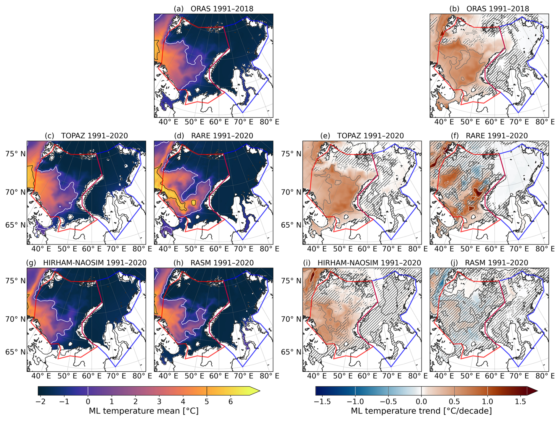
Figure A3 Average of mean ML temperature (left) and trend (right) of all the datasets in spring over the whole period. In the trend subplots, the not statistically significant area have been masked (“////” where p>0.1 and “…” where $\mathrm{0.05}<p<\mathrm{0.1}$).

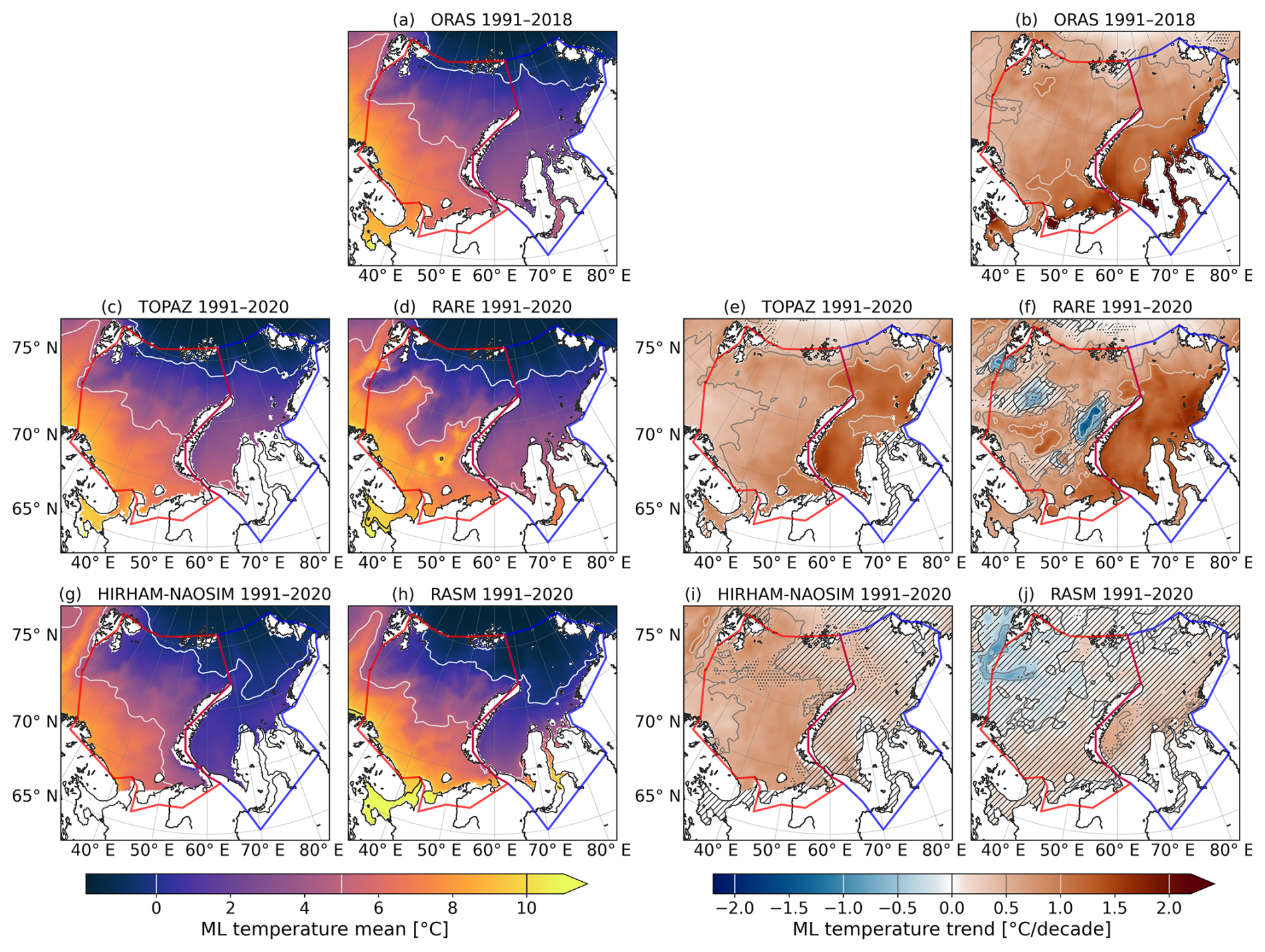
Figure A4 Average of mean ML temperature (left) and trend (right) of all the datasets in autumn over the whole period. In the trend subplots, the not statistically significant area have been masked (“////” where p>0.1 and “…” where $\mathrm{0.05}<p<\mathrm{0.1}$).

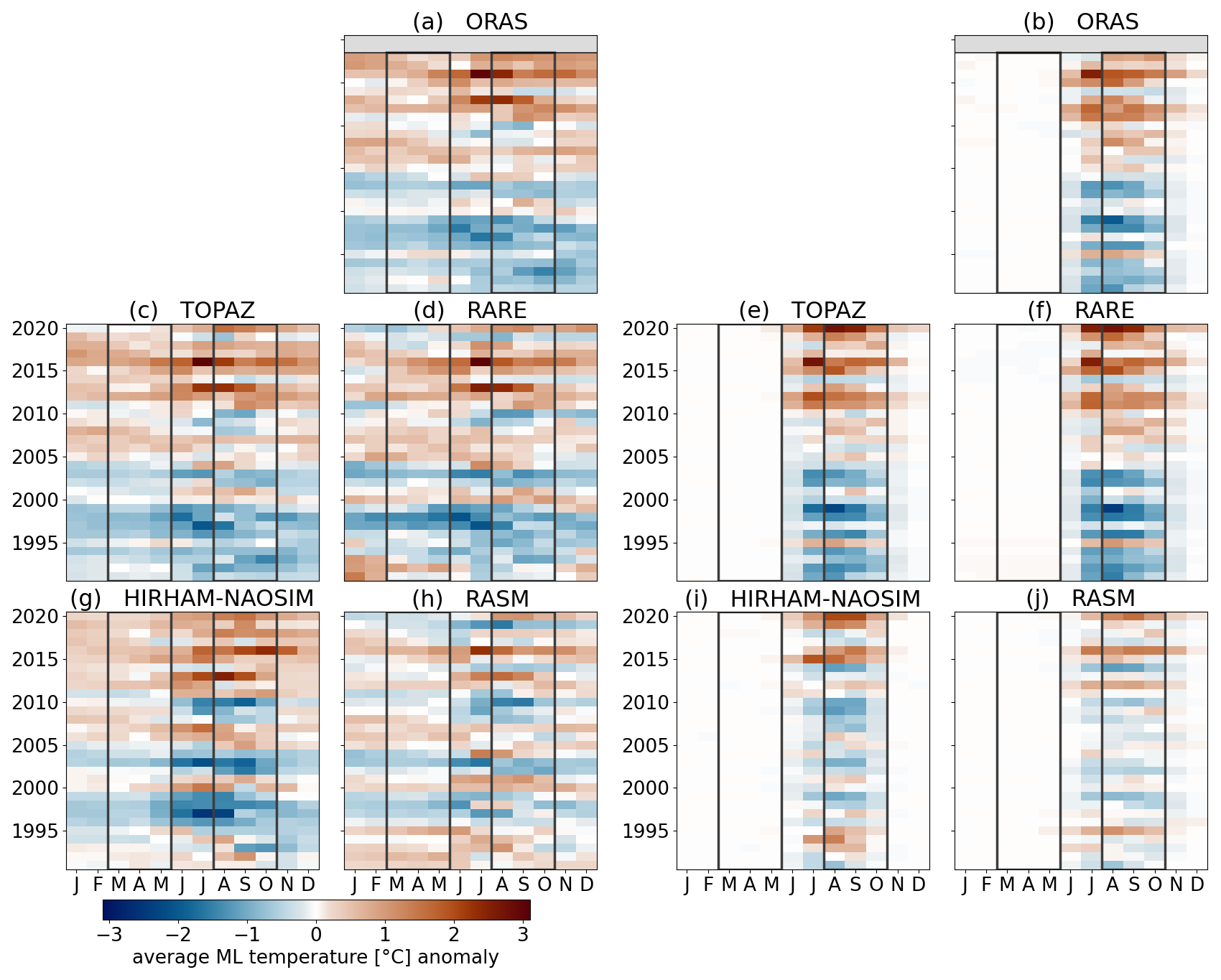
Figure A5 ML temperature anomaly in each model for the Barents (left) and Kara Sea (right). Spring and autumn seasons are marked with dark grey boxes. The anomaly is calculated by taking the difference from the monthly multiyear mean for each month. Note the different colour scales in the figures.

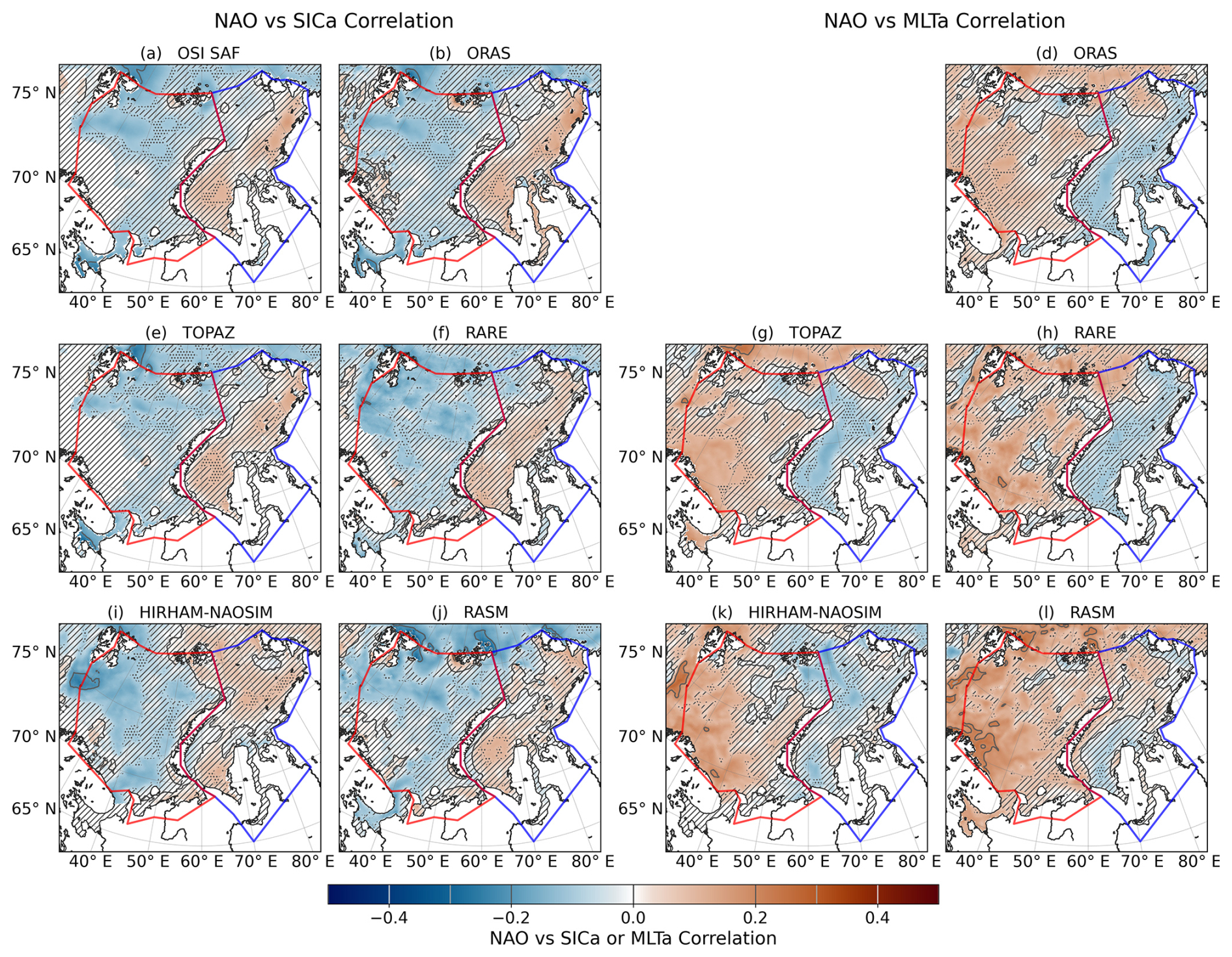
Figure A6 Correlation between climate index NAO and SIC anomaly (left) and MLT anomaly (right). The not statistically significant area have been masked (“////” where p>0.1 and “…” where $\mathrm{0.05}<p<\mathrm{0.1}$).

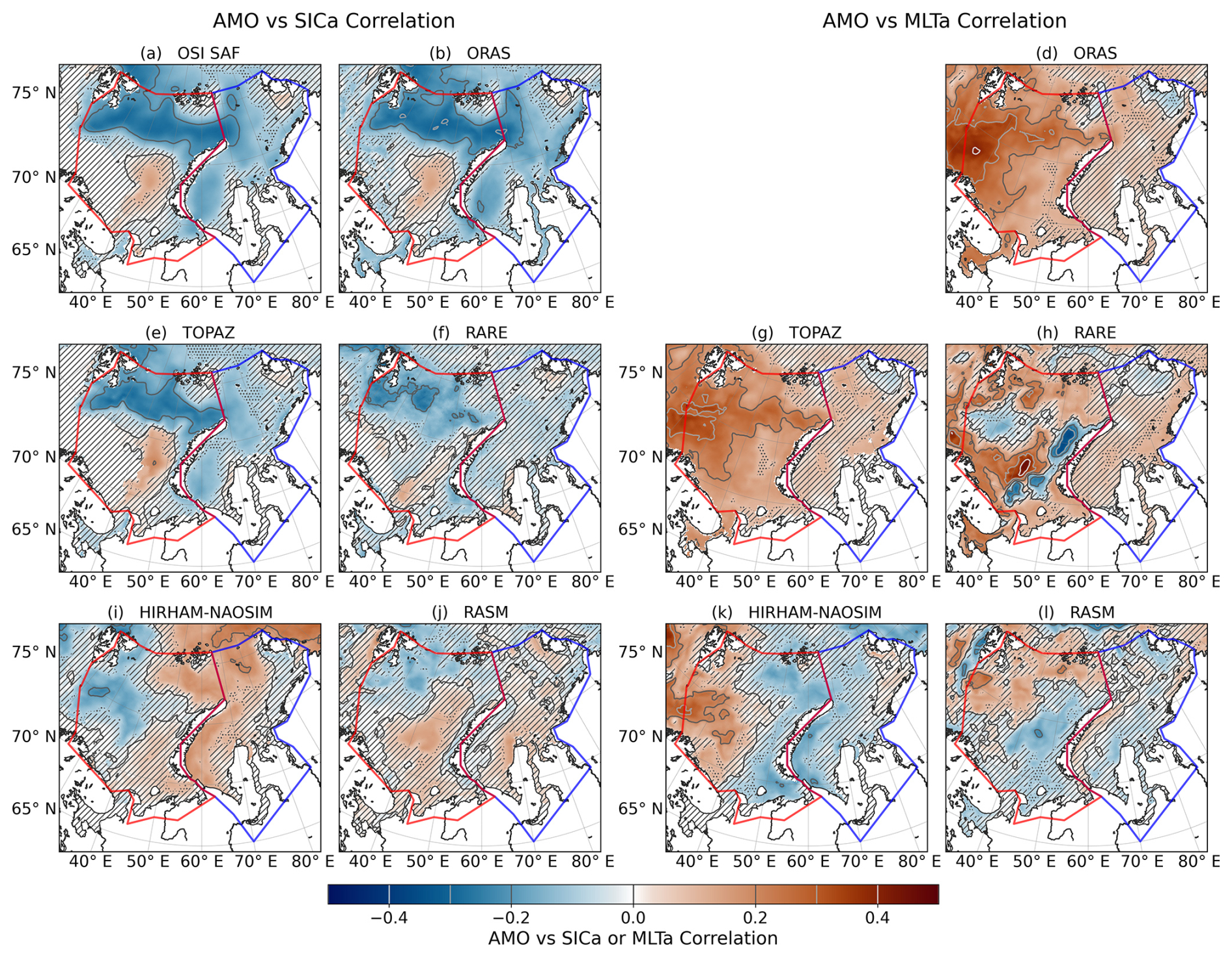
Figure A7 Correlation between climate index AMO and SIC anomaly (left) and MLT anomaly (right). The not statistically significant area have been masked (“////” where p>0.1 and “…” where $\mathrm{0.05}<p<\mathrm{0.1}$).

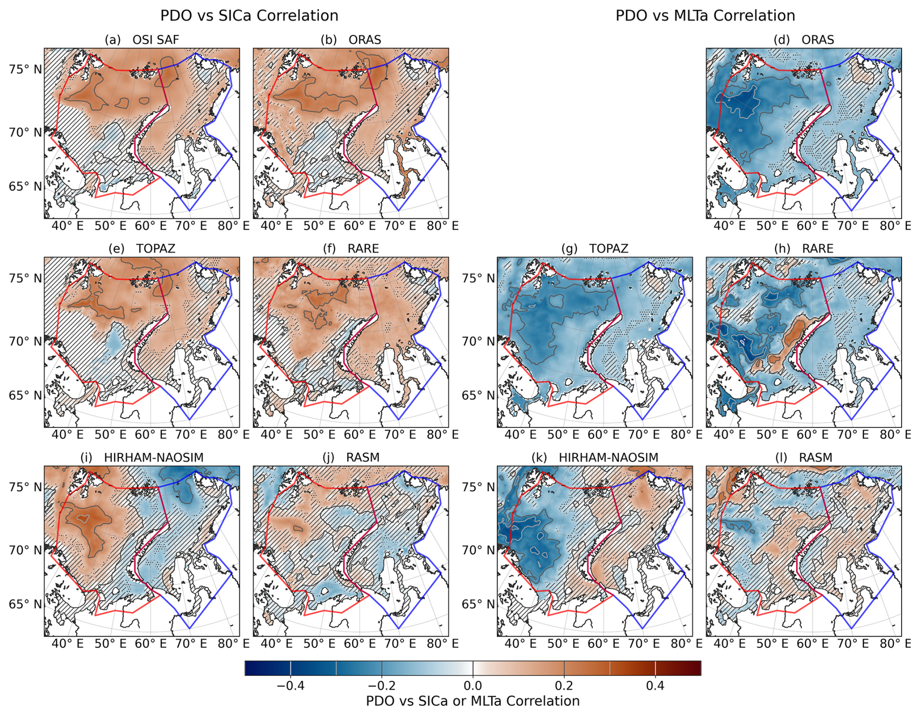
Figure A8 Correlation between climate index PDO and SIC anomaly (left) and MLT anomaly (right). The not statistically significant area have been masked (“////” where p>0.1 and “…” where $\mathrm{0.05}<p<\mathrm{0.1}$).

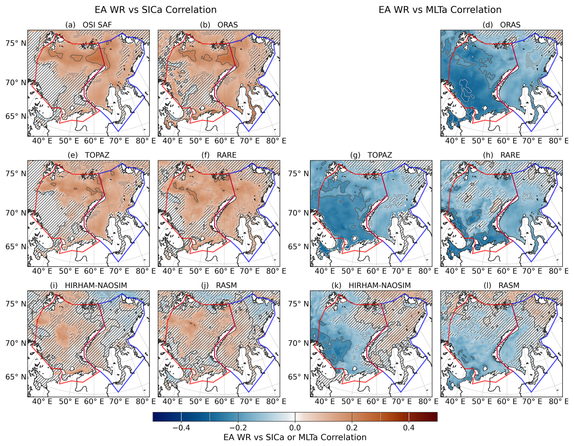
Figure A9 Correlation between climate index EA/WR and SIC anomaly (left) and MLT anomaly (right). The not statistically significant area have been masked (“////” where p>0.1 and “…” where $\mathrm{0.05}<p<\mathrm{0.1}$).

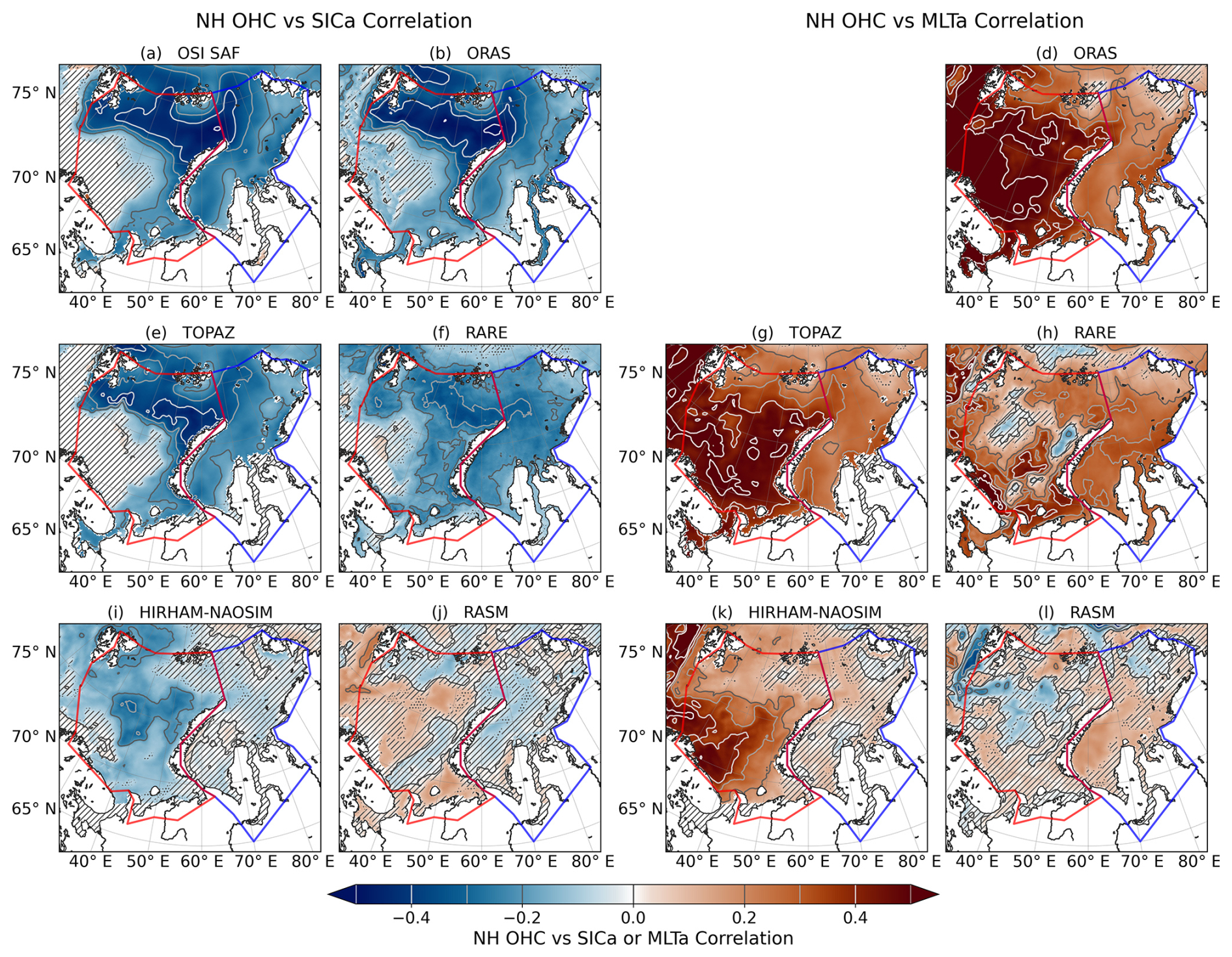
Figure A10 Correlation between climate index NH OHC and SIC anomaly (left) and MLT anomaly (right). The not statistically significant area have been masked (“////” where p>0.1 and “…” where $\mathrm{0.05}<p<\mathrm{0.1}$).