Impact of waves on phytoplankton activity on the Northwest European Shelf: insights from observations and km-scale coupled models

The spring bloom is an annual event in temperate regions of the North Atlantic Ocean where the abundance of photosynthetic plankton increases dramatically. The timing and intensity of the spring bloom is dependent on underlying physical conditions that control ocean stratification and mixing. Although surface waves can be an important source of turbulent kinetic energy to the surface mixed layer, they have seldom been considered explicitly in studies of bloom formation. Here, we investigate the role of surface waves in bloom formation using a combination of satellite observations and numerical models. Satellite observations show a positive correlation between wave activity and chlorophyll concentration in the Northwest European shelf (May–September). In the deeper Northeast Atlantic, increased wave activity correlates with lower chlorophyll during periods of high phytoplankton activity (March-May) and higher chlorophyll when activity is low (below 54° N, July–September). We use a first-of-its-kind, km-scale, two-way coupled ocean-wave model system to investigate both the relationship between wave-driven mixing and bloom formation, and the sensitivity of model results to the method by which wave-driven mixing is parameterised. In deep regions, during the spring bloom, a wave-driven mixing event is likely to mix surface chlorophyll to deeper layers, away from light. In contrast, when phytoplankton activity is low in deep regions, wave-driven mixing can entrain nutrients, fueling the growth of nutrient starved phytoplankton near the surface. In June–October, in shallow but weakly stratified regions of the shelf, surface chlorophyll tends to be elevated following a wave-driven mixing event, which can bring to the surface both phytoplankton and nutrients from deeper layers. When contrasted with ocean-only runs, the two way-coupled ocean-wave model tends to produce greater vertical mixing and a delay in bloom onset. These results indicate bloom dynamics are sensitive to the way in which waves are modelled, and that the role of waves in bloom formation should be considered in future studies.

1 Introduction

The spring bloom is a defining feature of annual marine primary production in temperate waters of the Northeast Atlantic and adjoining shelf seas. It is characterised by a rapid increase in the abundance of phytoplankton–photosynthetic microorganisms that are the ocean's dominant primary producers. Following winter, the spring bloom provides the first major influx of food for the rest of the marine food web, and many organisms have adapted their development to take advantage of the increased food supply (Cushing, 1990; Ji et al., 2010; Cyr et al., 2024). The spring bloom is tightly linked to changes in the physical environment at the end of winter; a link first identified by G. A. Riley in the early 1940s (Riley, 1942). However, the exact trigger for the spring bloom is still debated. Sverdrup proposed the Critical Depth Hypothesis, which states that the spring bloom occurs when the thermocline rises above a critical depth (Sverdrup, 1953). Sverdrup's critical depth is the maximum depth a phytoplankton cell can be mixed down to while still receiving enough light to offset losses associated with respiration and other processes. When the thermocline is above the critical depth, phytoplankton cells are trapped in well-lit, nutrient-replete waters near the surface where conditions are favourable for growth and reproduction.

Another proposed explanation for the timing of bloom formation is the Critical Mixing Hypothesis, which states that a bloom can form in a mixed water column if the rate of mixing is low enough for phytoplankton near the surface to achieve net positive growth (Huisman et al., 1999). This mechanism was explored by Taylor and Ferrari (2011) using high resolution, three-dimensional ocean models, with a reduction in net cooling at the end of winter identified as a key trigger. Biological controls on bloom formation have also been proposed, including the Dilution-Recoupling hypothesis, which focuses on the balance between phytoplankton growth and grazing pressure through winter and into spring (Behrenfeld, 2010). Although the exact mechanism controlling bloom formation is still debated, a recent study using autonomous underwater gliders lent most support to Sverdrup's Critical Depth Hypothesis based on the depth of active mixing (Rumyantseva et al., 2019).

In tidally active areas on the continental shelf, stratification and bloom formation are also dependent on the water depth and the degree of mixing in the bottom boundary layer. Shallow regions of the Northwest European Shelf (NWES), including areas in the English Channel and the southern North Sea, remain permanently mixed year round (van Leeuwen et al., 2015). Other areas may be intermittently stratified, depending on prevailing tidal and atmospheric conditions. The bloom itself can be interrupted by an increase in bottom mixing associated with the spring-neap tidal cycle, or the passage of a storm, leading to an apparent double bloom (Sharples et al., 2006).

Once established in deeper waters, stratification can be difficult to break down, requiring extreme atmospheric conditions, such as those associated with the passage of a hurricane or typhoon, to fully mix the water column (Shi and Wang, 2007; Babin et al., 2004; Sharples et al., 2001). Such events can trigger a new bloom in their wake, fuelled by a fresh influx of nutrients that have been mixed up from below the nutricline. In the absence of an extreme mixing event, the bloom will often peak before reducing in intensity as the supply of nutrients is exhausted and top-down pressures from grazing and viral lysis take hold (Simpson and Sharples, 2012). Near the nutricline, given sufficient light, it is common for a sub-surface chlorophyll maximum to form in the summer. As stratification begins to break down at the end of summer, an autumnal bloom can sometimes be observed.

While the spring bloom is an annual event, its timing, duration and intensity exhibit significant inter-annual variability. Using models driven at the surface by winds and changes in the net heat flux, Waniek (2003) showed the spring-time shallowing of the mixed layer can be interrupted by mixing events caused by weather systems whose frequency and intensity vary from year to year, leading to inter-annual variability in bloom dynamics. This is a result that is embedded in contemporary coupled hydrodynamic-biogeochemical models, which are typically forced at the surface by a set of common variables, including wind, surface pressure, surface temperature, net short-wave radiation and fresh water fluxes.

One aspect that isn't typically considered in studies of bloom dynamics is the impact of surface waves on turbulent mixing, despite evidence that bloom timing can be closely coupled to meteorological indices (Powley et al., 2020). The impact of waves on the ocean may either be parameterised in an ocean only model, or modelled explicitly using a combination of ocean and wave models in a two-way coupled configuration. In ocean only models the input of turbulent kinetic energy at the ocean surface often follows the assumption that wind and waves are in equilibrium with each other, which is only valid under certain wind regimes and in the deep open-ocean, far from coastlines (Cavaleri et al., 2012). This then influences the effects of surface waves, e.g. Langmuir turbulence (Li et al., 2019). Surface waves also induce Lagrangian drift in their direction of propagation, known as Stokes drift (Phillips, 1977; Stokes, 1847) – a process not usually taken into account in stand-alone ocean models. Wave breaking terms and their impact on the vertical eddy diffusivity are sometimes considered, but often include assumptions relating to the water-side momentum flux (Craig and Banner, 1994) and surface roughness calculations; with the wave-age and significant wave height estimated as functions of the water-side friction velocity (Rascle et al., 2008).

Traditionally, models for different components of the Earth system – the atmosphere, land, ocean and ocean waves – have been run independently. However, with improvements in computing power, studies using two-way coupled model configurations are becoming increasingly common (Berthou et al., 2025). Recent studies have shown the benefits of coupling a wave model to an ocean model to derive these terms more accurately in high resolution configurations (Lewis et al., 2019; Bruciaferri et al., 2021; Valiente et al., 2021). This has led to improvements in the forecasting of extreme wave heights and surges, ocean mixing (Lewis et al., 2019), and surface currents (Bruciaferri et al., 2021). Replacing the parameterised calculation of wave variables by an explicit wave model through coupling can have variable effects depending on the wave momentum calculation in the stand-alone ocean model set-up: in the case of Lewis et al. (2019), which used a similar set up to our study, two-way coupling tended to enhance vertical mixing, leading to a deeper summer mixed layer, resulting in a relative cooling of surface and upper ocean temperatures during periods of stratification. In the case of Alari et al. (2016) and Breivik et al. (2015), the impacts of wave coupling on the ocean tended to reduce summer mixing and generated enhanced upwelling in the Baltic Sea due to the additional Stokes drift. This highlights the value of wave coupling, but also the need to modify turbulence parametrisation schemes in ocean models to account for wave coupling (Couvelard et al., 2020).

Wave-induced mixing has been observed to impact phytoplankton dynamics when included in coupled hydrodynamic-biogeochemical models, both by delaying the spring phytoplankton bloom and enhancing chlorophyll-a levels at the surface and at depth (Liu et al., 2025; Tensubam et al., 2024). In this study, we investigate the sensitivity of bloom timing and ecosystem processes across the NWES and the Northeast (NE) Atlantic by coupling a wave model to an ocean-biogeochemistry model. This region is located at the end of the northern and central branches of the North Atlantic storm track (Woollings et al., 2010), and is therefore subject to high wave activity in the winter, and episodic wave activity in summer. The NWES is also an extremely productive region, with a pronounced spring bloom evident over large areas of the shelf (Simpson and Sharples, 2012). Specifically, we address the following questions: (i) What is the relationship between wave activity and phytoplankton bloom phenology? (ii) How sensitive are model results to the parameterised and explicit representation of wave fields?

For this study, we use the UK Met Office's operational ocean-wave coupled model system, which has been extended by coupling it to the European Regional Seas Ecosystem Model (ERSEM) (Butenschön et al., 2016). The new system allows for two-way feedbacks between each model component to be represented, providing a more realistic representation of surface mixing and ecosystem responses. This representation contains several wave-induced processes that are absent from the non-coupled system, namely Stokes drift, growing/decaying waves and surface mixing influenced by wave fields. The study represents the first time a coupled ocean-wave-biogeochemistry model at km-scale resolution has been used to simulate ecosystem processes across the NWES and NE Atlantic. The modelling work is complemented by an analysis of both satellite and in-situ observations.

The plan for the paper is as follows. In Sect. 2, we describe the study area and quantify relationships between satellite ocean colour and wave reanalysis data for recent decades. We then focus on the year 2018, when three named storms passed over the UK between the months of June and September, and examine the temporal evolution of phytoplankton abundance over the course of the year. In Sect. 3, we describe the modelling tools which we use to simulate the year 2018, showing the results of the modelling study in Sect. 4. In Sect. 5, we use the models and observations to compare bloom phenology and ecosystem responses to summer wave activity, and investigate the impacts that wave coupling has on ocean physics and biogeochemistry. Finally, in Sect. 5.3, we bring the modelling and observation results together to propose mechanisms for the phytoplankton activity response to wave activity shown in Sect. 2.

2 The Northwest European Continental Shelf and North East Atlantic

2.1 Physical and hydrodynamic characteristics

The NWES is a broad temperate continental shelf on the eastern side of the North Atlantic Ocean (Fig. 1). The region is demarcated by the shelf break, which extends north-westward through the Bay of Biscay in the south, along the edge of the Armorican shelf and up and around the west coasts of Ireland and Scotland, then north-eastward toward the west coast of Norway. Topographic steering drives the northward flow of water parallel to the shelf slope, with more limited cross-slope transport driven by surface winds and meandering eddies. Off-shelf, in the north of the region, the North Atlantic Current flows north-eastward between Iceland and Scotland. Water enters the North Sea in the north through central and western regions of the northern North Sea, and in the south through the English Channel. The dominant outflow from the North Sea is via the Norwegian Coastal Current.

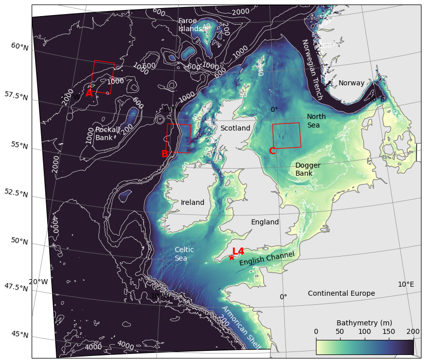
Figure 1 AMM15 model domain extent with bathymetry contours (m). Red boxes highlight representative analysis zones for off-shelf (A), shelf break (B) and on-shelf (C) areas. The L4 monitoring station is shown with a star.

On-shelf, dynamics are controlled by seasonal changes in solar irradiance and heating, atmospheric fluxes and wind forcing, tides, river inputs and exchanges with the open ocean. Large areas of the shelf are seasonally stratified, including in the Celtic Sea, western reaches of the English Channel and the central North Sea. Shallower areas on the shelf may be intermittently stratified or permanently mixed, with tidal mixing fronts separating stratified and well mixed areas. Nutrient concentrations are influenced by exchanges with the open ocean, atmospheric deposition and, particularly in coastal areas, river discharge. Bottom-up controls on the growth of phototrophic plankton include the availability of light and nutrients; and temperature. The spring bloom typically occurs from late March into April (Racault et al., 2012), and tends to start in the south of the domain before spreading northward. In coastal waters with high sediment loads, the growth of surface plankton can be light limited. In the summer, under stratified conditions, surface phytoplankton become nutrient limited.

2.2 Monthly wave energy relationship to observed chlorophyll concentration in climatology

To explore the potential impact of waves on bloom dynamics in the NE Atlantic and on the NWES, we examine satellite ocean colour and wave reanalysis data. We used chlorophyll-a from the Ocean Colour Climate Change Initiative (OC-CCI) dataset (Sathyendranath et al., 2019, 2023) and wave energy from the Met Office regional wave hindcast from WAVEWATCH III (Saulter, 2024) to calculate inter-annual correlations between bimonthly-mean chlorophyll concentrations and wave energy from 1998–2020. To achieve this, the temporal mean was calculated across pairs of months for each year from March–November, when the majority of primary production occurs. Wave energy and chlorophyll data were then normalised at each spatial pixel and the Pearson correlation coefficient calculated between them, with significance tested using a two-sided p-value for the correlation being different to zero (Virtanen et al., 2020).

The results show a strong negative correlation between wave energy and chlorophyll concentration off-shelf and near the shelf break in March–May, and a strong positive correlation on-shelf from June–October (Fig. 2). This suggests that stronger wave activity in the open ocean when phytoplankton are blooming in March–May leads to a reduction in surface chlorophyll, whilst the reverse is true on-shelf later in the year. Off-shelf, the response to enhanced wave activity appears positive in the south-west of the domain from June to September. In the north-west of the domain, the open-ocean response is confined to close to the shelf break and, where significant, is generally negative, except in August-September. Wave energy is likely not the sole causal factor in this correlation: increased storminess will also decrease available sunlight.

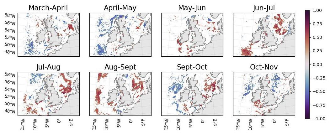
Figure 2 Correlation between mean wave energy and mean chlorophyll concentration from 1998–2020 for different pairs of months. Only regions where the correlation coefficient is significant (p<0.1) are coloured. Wave data is from a WAVEWATCH III reanalysis (Saulter, 2024) and chlorophyll satellite data is from OC-CCI (Sathyendranath et al., 2019, 2023).

2.3 Wave activity and chlorophyll concentration in 2018

The year 2018 has been selected for this study as there was a cooler ocean surface in March–April, when the spring bloom typically occurs, and enhanced wave activity compared to climatological conditions (Fig. 3). Later in the year, two marine heatwaves (MHW) developed. The first was in late May to mid-June and the second in July. The first was terminated by storm Hector, which passed over the UK between 13 and 14 June 2018, particularly impacting the North of the UK and Ireland. The second heatwave was terminated by an unnamed storm which passed over the UK on 29 July. Storm Ali and Bronagh passed over the UK in succession between 18 and 21 September.

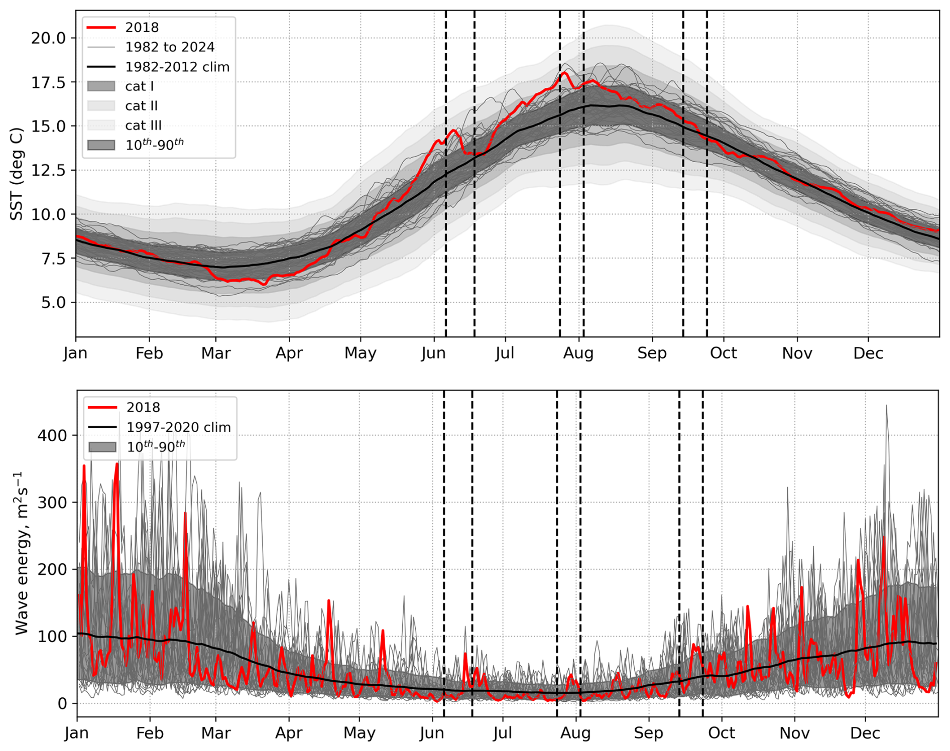
Figure 3 Top – Operational Sea Surface Temperature and Ice Analysis (OSTIA) SSTs for 1982–2022, mean climatology for the time period used to define marine heatwave thresholds (1982–2012) in bold, 10th–90th percentiles (anomalies smoothed with 31 d moving average), Shading: Category I, Category II, Category III marine heatwaves using Hobday et al. (2018) averaged over the NWS. Bottom – Wave energy from Met Office wave regional reanalysis (Saulter, 2024) for 1997–2020. Yearly data shown with grey lines, mean climatology from 1997–2020 in black, 2018 in red. Grey shading between 10th–90th percentiles. Mean and percentiles smoothed with 31 d moving average. Wave energy averaged over the NWS (NWS = blue + purple regions in Fig. 1). Vertical dashed lines indicate three key 2018 storm periods.

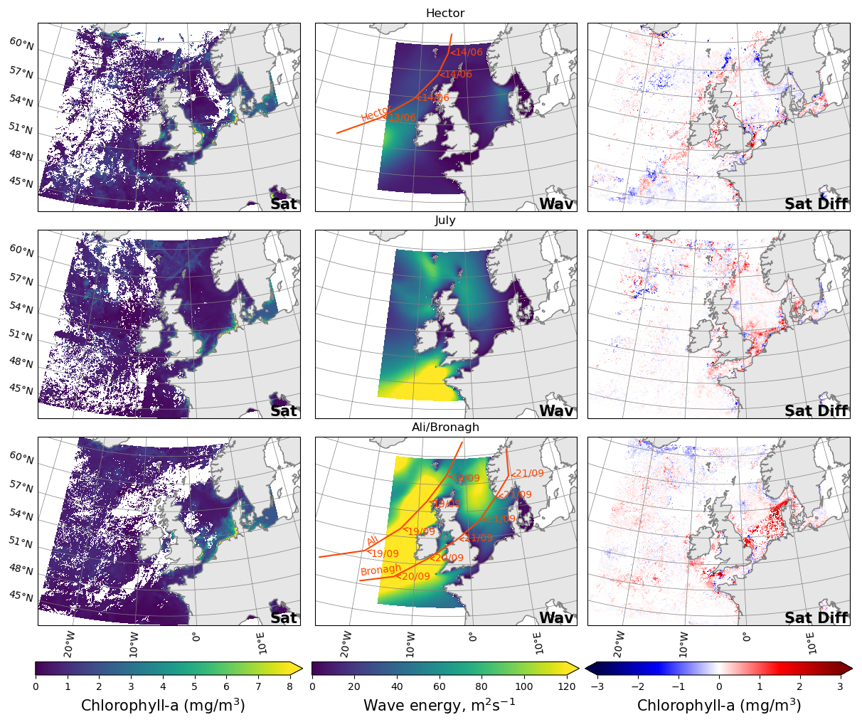
Figure 4 Mean chlorophyll from satellite in the five days before the storm (left), wave activity on the day of the storm from the Met Office wave regional reanalysis (Saulter, 2024) (middle) and difference in the mean satellite chlorophyll five days after and before (right) storm Hector (top), July storm (middle) and storms Ali and Bronagh (bottom). The start of the five days before and the end of the five days after the storms are highlighted in Fig. 3 as vertical bars.

Late summer storms can either suppress or enhance chlorophyll, depending on timing and area (Fig. 4). In June, as a result of storm Hector, the concentration of chlorophyll was reduced in northern off-shelf areas, which were in bloom state, whereas chlorophyll increased on the western part of the shelf in regions which were past their bloom state. Particularly strong increases are noticeable in the Celtic Sea, Irish Sea, and Southern North Sea. Following the July storm, chlorophyll concentration was low off-shelf and the storm had a minimal impact. In contrast, the concentration increased in coastal areas of the shelf. In September, northern areas tended to see a decrease in chlorophyll from storms Ali and Bronagh, whilst southern and on-shelf areas saw a strong increase.

The observations confirm 2018 to be an interesting year to study the relationship between wave activity and the concentration of chlorophyll. Indeed, some years have uninterrupted summer stratification (e.g. 2017, used in Lewis et al., 2019): we choose a year in which wave activity was enhanced in spring and had intense summer wave activity events able to disrupt the ocean stratification. In the remainder of the article, we focus on how intense periods of wave activity affected the concentration of chlorophyll, and how explicitly coupling an ocean model to a wave model impacts model results.

3 Model framework

The impact of ocean-wave coupling on biogeochemistry is assessed through a twin experiment. Experiments are conducted with (WAV) and without (OCN) the coupled wave model in order to examine the biogeochemical response, as shown in Scheme 1.

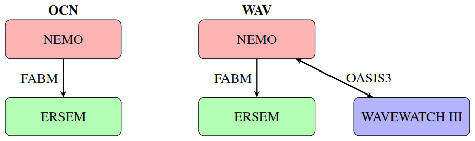
Scheme 1 Schematic of the twin experiments with two-way coupling between the ocean and wave components and one-way coupling between the ocean and biogeochemistry.

3.1 Hydrodynamic model

Both simulations have been performed using the Nucleus for European Modelling of the Ocean (NEMO) model (Gurvan et al., 2019), adapted for simulating shelf sea dynamics (O'Dea et al., 2012). For this study, we use NEMO v4.0.4. The model domain is the high-resolution 1.5 km Atlantic Margin Model (AMM15) configuration (Fig. 1), which is used for operational forecasting by the UK Met Office (Tonani et al., 2019). In contrast to the more commonly used 7 km configuration for the same region (AMM7), the high resolution domain better resolves smaller scale processes such as eddies, fronts and internal waves (Graham et al., 2018a, b), all of which can influence wave activity.

Initial fields for the simulations were provided by a previous ocean-wave experiment (Lewis et al., 2019), with lateral boundary forcing from global ocean models. Meteorological forcing is provided at 3 hourly intervals from the UK Met Office global Unified Model analysis, at a 25 km resolution. There is no live coupling from sea-surface back to the atmosphere.

For the uncoupled OCN simulation a limited, parameterised version of waves are included in the following way (see Reffray et al., 2015, for full details about the NEMO implementation):

1. Sea surface roughness is approximated as a function of the estimated significant wave height based on wind speed, as proposed by Rascle et al. (2008);

2. Water-side momentum flux (i.e., the wind stress τ_atm) is completely transferred into the ocean;

3. Vertical eddy viscosity is computed using the two-equation GLS turbulent closure model, taking into account:

   • a.

     parameterised surface enhanced mixing due to wave-breaking (Craig and Banner, 1994), a function of water-side friction velocity depending on wind stress;

   • b.

     Sea surface roughness z₀, estimated as above.

3.2 Wave model

To better resolve waves effects, NEMO is coupled to a regional implementation of the WAVEWATCH III spectral wave model version 4.18 (Tolman, 2014) as detailed in Saulter et al. (2017). The domain, AMM15-wave, covers the same extent as the AMM15 NEMO model but uses a Spherical Multiple Cell discretization scheme (Li, 2012) configured to have a variable horizontal resolution ranging from 3 km across much of the domain down to 1.5 km near the coast or where the average depth is shallower than 40 m. Wave growth and dissipation terms are parameterised following Filipot et al. (2010) while non-linear wave-wave interactions use the Discrete Interaction Approximation (DIA) package according to Hasselmann et al. (1985).

Two-way coupling utilises the OASIS3-MCT coupler (Valcke et al., 2015). NEMO shares water levels and currents with the spectral wave model. In turn, WAVEWATCH III injects Stokes drift, significant wave height and water-side momentum flux into the hydrodynamic model. The coupling frequency is hourly.

By explicitly coupling WAVEWATCHIII to NEMO, as in the WAV experiment, the ocean momentum budget equation is modified to include three wave feedbacks as described in Bruciaferri et al. (2021).

1. Surface waves induce a mean Lagrangian drift in their direction of propagation known as Stokes drift (e.g., Phillips, 1977; Stokes, 1847). When the wave-induced drift interacts with the planetary vorticity, an additional force named the Coriolis–Stokes force (CSF) appears in the wave-averaged Eulerian momentum equation (Hasselmann, 1970). Stokes Drift at the surface is computed by the wave model and exchanged with the ocean model together with the significant wave height and the mean wave period, so that the ocean model can calculate the depth-varying 3D Stokes drift according to Breivik et al. (2016);

2. Wind blowing on the sea surface generates both ocean waves and currents. As a result, sheared ocean currents are directly forced by the total wind stress, τ_atm, only in the case of fully developed wind-waves (Pierson and Moskowitz, 1964). Most of the time, the wave field is far from being in equilibrium with the local wind, and waves are either growing, with a net influx of momentum into the wave field, or decaying, with intensified wave-breaking and a net outflux of momentum from waves into the ocean (e.g., Komen et al., 1994). Thus, when surface waves are considered the water-side momentum flux τ_ocn (i.e., the stress that effectively forces the ocean at the surface) is given by:

   $$\begin{array}{}\text{(1)}& {\mathit{\tau }}_{\text{ocn}}={\mathit{\tau }}_{\text{atm}}-{\mathit{\tau }}_{\text{atw}}+{\mathit{\tau }}_{\text{woc}}\end{array}$$

   where τ_atw is the momentum flux absorbed by the waves (or the wave-supported stress) and τ_woc is the momentum flux from the wave field to the mean flow. In the wave-ocean coupled model, τ_woc is computed by the wave model and directly passed to the ocean model;

3. Vertical eddy viscosity is still computed using the two-equation GLS turbulent closure model (Reffray et al., 2015), with the following changes:

   • a.

     Surface enhanced mixing now dependent on τ_woc instead of τ_atm,

   • b.

     Sea surface roughness as a function of the significant wave height provided by the wave model.

Due to limitations of the GLS turbulence scheme there are some processes that WAVEWATCH III resolves which are not currently configured to directly influence the ocean model through coupling. These include the effect of wave breaking on the surface turbulent kinetic energy budget (following Craig and Banner, 1994) and explicit treatment of Langmuir turbulence, (e.g. through use of a vortex-force formulation (Uchiyama et al., 2010), ocean bed stress linked with wave/current interactions (Zhang et al., 2022) or enhanced vertical mixing (Li et al., 2019)).

In this study the inclusion of wave feedback in NEMO through WAVEWATCH III in the WAV simulation is referred to as explicit wave coupling, whilst the standard approach of NEMO in the OCN simulation is referred to as parameterised waves.

3.3 Biogeochemical model

For this study, we use the European Regional Sea Ecosystem Model (ERSEM) for simulating ocean biogeochemistry and phytoplankton bloom dynamics (Butenschön et al., 2016). ERSEM has been coupled to NEMO using the Framework for Aquatic Biogeochemical Models (FABM, Bruggeman and Bolding, 2014). FABM facilitates passing data between biogeochemical and hydrodynamic models. Here, the coupling is one way, and the biogeochemical model does not feedback onto ocean physics. Whilst ERSEM is not directly coupled to the wave model, biogeochemical processes are influenced by changes in ocean currents and mixing that are caused by the wave model.

This is the first instance of ERSEM being used with the NEMO AMM15 domain. Initial values are interpolated from a reanalysis run performed on the coarser AMM7 domain for November 2016. Since the north-west corner of the AMM15 region extends beyond the bounds of the AMM7 domain, extrapolation is performed using a simple nearest neighbour algorithm. Before performing the 2018 experiment, a fourteen month ocean-biogeochemistry only simulation starting on 1 November 2016 is used to “spin-up” the biogeochemical initial conditions and negate any impact of extrapolation.

A constant supply of non-depleting nutrients at the boundary can lead to spurious phytoplankton blooms and other unrealistic responses. This is mitigated by enforcing a constant value matching the near-zero winter values at the boundary for most of the previously unconstrained tracer fields following the guidance in Polton et al. (2023). Biogeochemical surface boundary conditions include nitrogen deposition from the atmosphere and light attenuation due to detritus and yellow matter (the Gelbstoff absorption coefficient). Nitrogen deposition data is available at monthly resolution using models run by the European Monitoring and Evaluation Programme (EMEP) (Simpson et al., 2012), which are then converted into fluxes for both oxidised and reduced components. The Gelbstoff absorption coefficient is produced using data from OC-CCI (Sathyendranath et al., 2019), for a multitude of wavelengths that are integrated into a single broadband field.

River input data is an updated version of the files used in the CMEMS north-west European shelf reanalysis from Lenhart et al. (2010). A climatology from the Global River Discharge Database (Vörösmarty et al., 2000) and data from the Centre for Ecology and Hydrology (Young and Holt, 2007) have been used to provide time varying daily river discharge, nutrient loads (nitrate, ammonia, phosphate and silicate), total alkalinity, dissolved oxygen and dissolved inorganic carbon.

4 Modelling results

4.1 Validation

In Lewis et al. (2019) and Graham et al. (2018a, b), a detailed validation of the physical ocean and wave models has been performed, demonstrating good performance of stand-alone models and improvements to significant wave height and total water level extremes when coupling ocean and waves (Lewis et al., 2019). For biogeochemistry, while there have been several modelling studies using ERSEM on the coarser AMM7 domain (e.g. Jardine et al., 2022; Powley et al., 2024), this experiment is the first simulation of ERSEM biogeochemistry on the 1.5 km regional domain.

Profiles of temperature extracted from the EN4 Met Office Hadley Centre Observation Dataset (Good et al., 2013) were compared to predicted profiles of temperature from both the OCN and WAV models for March–June (Fig. 5) in off-shelf areas deeper than 200 m. Both models show a persistent warm bias off-shelf, which is due to the combination of surface forcing that itself has a warm bias and model drift before the start of our 2018 simulations. The coupling of waves results in a marginal improvement during spring when the water column is well mixed, but as it stratifies in June the impact of waves increases leading to a reduction in the overall bias.

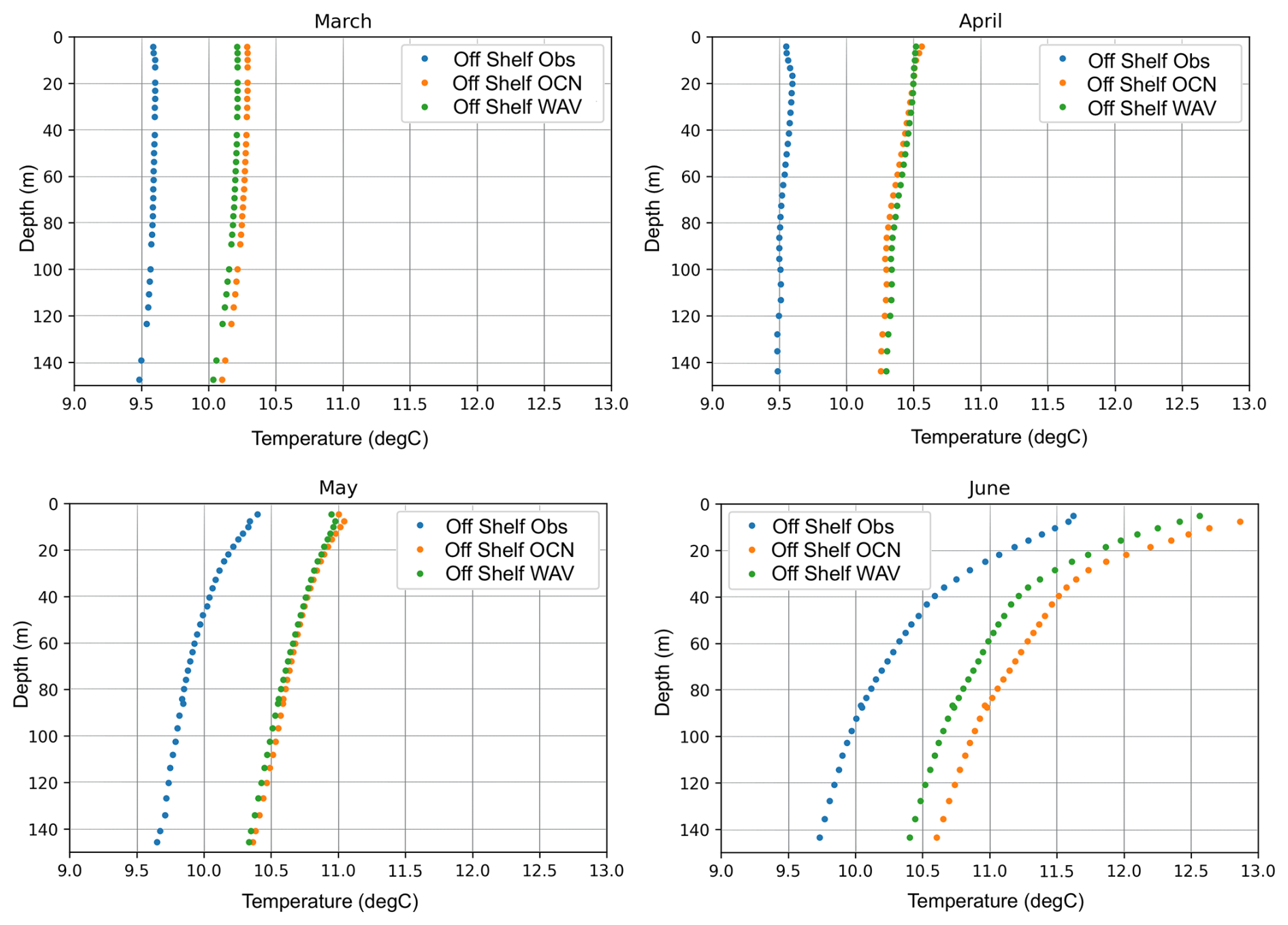
Figure 5 Potential temperature profiles within the off-shelf region, averaged over all observed profiles in the EN4 database that are located within 1.5 km of a model grid cell for March, April, May and June (blue), along with the corresponding simulated profiles at the same point and time for the OCN (orange) and WAV (green) simulations.

The warm bias for temperature is also present when compared to satellite surface fields from the Operational Sea Surface Temperature and Ice Analysis (OSTIA) (Fig. 6), with a persistent positive bias across most of the domain. The warm bias results in a combination of higher phytoplankton growth rate and a higher rate of mineralisation of summer nutrients. Therefore it is no surprise to also see a positive bias across most of the off-shelf domain for chlorophyll compared with OC-CCI surface satellite measurements for 2018 (Fig. 6). Unlike temperature, on-shelf and coastal areas have a negative bias with the greatest values in areas close to river mouths. In part, the bias is a result of using climatological river input data, which prevents the model from capturing inter-annual variability in river inputs and their impact on ecosystem dynamics.

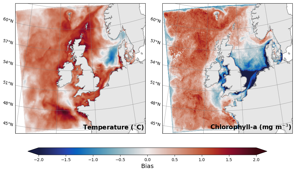
Figure 6 Annual mean bias at the surface between the ocean-only model and (left) satellite temperature from OSTIA, or (right) chlorophyll from OC-CCI.

For in-situ observations of biogeochemical variables, we use data from the long-term monitoring site Station L4 (McEvoy et al., 2023), which is located on the western edge of the English channel (Fig. 1). This site contains valuable observational data, albeit in a region where wave activity does not have a significant impact. Figure 7 shows a comparison of the two simulations with observations for surface temperature, salinity and chlorophyll-a from Station L4. Also plotted are Net Primary Production (NPP) from both model runs and Significant Wave Height from the WAV simulation. Temperature is consistent between the models, with the warm bias vs. observations evident over the winter months (Fig. 7a). The effect of the marine heatwaves is clearly visible in the observations, whilst the response in the models is more muted. In winter months, the WAV model is more saline at the surface (Fig. 7b), indicating greater mixing of buoyant, freshwater inputs from the river with more saline waters. These periods typically correspond to times of higher wave activity (Fig. 7e). Low salinity events seen in the observations are missed due to the use of climatological rivers missing high rainfall events. The inclusion of waves has only a minor impact on the spring bloom at this location (Fig. 7c), with slower initial growth and a slightly delayed peak. For most of the year the models over predict the chlorophyll, consistent with the findings in Fig. 6. The models also miss the late bloom in August that appears in-situ observations, although there is no evidence in the satellite measurements of a bloom at this time.

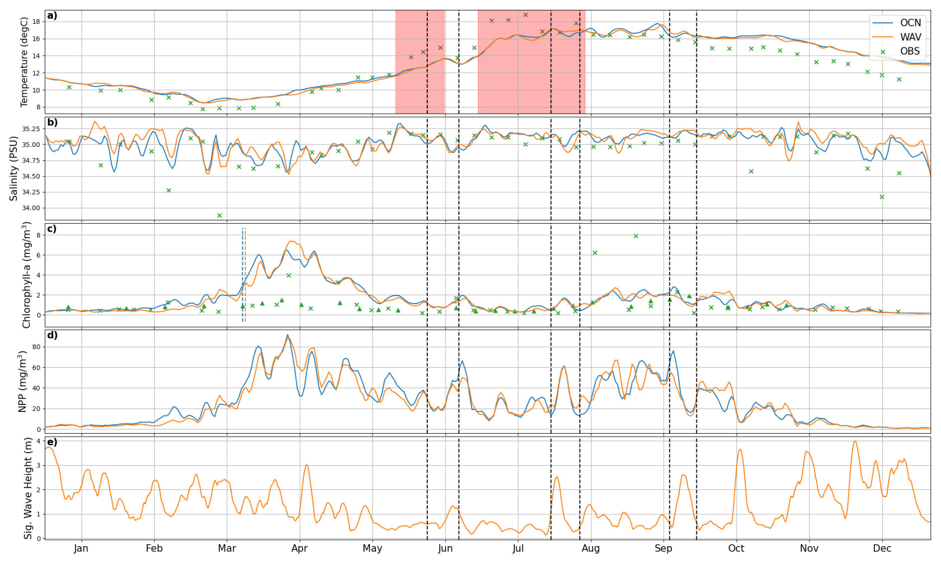
Figure 7 Surface comparison of modelled and observed biogeochemical variables at the L4 station (Fig. 1). Observations are from the Western Channel Observatory (McEvoy et al., 2023), with the addition of OC-CCI satellite chlorophyll (triangles). Red zones indicate ocean heat waves, black vertical dashed lines denote the storm times and the blue/orange vertical lines are the estimated bloom onset time.

Whilst the use of biased surface forcing prohibits an in depth comparison between the model and observations, the use of a twin experiment enables us to evaluate the impact of wave processes through explicit coupling from a mechanistic perspective.

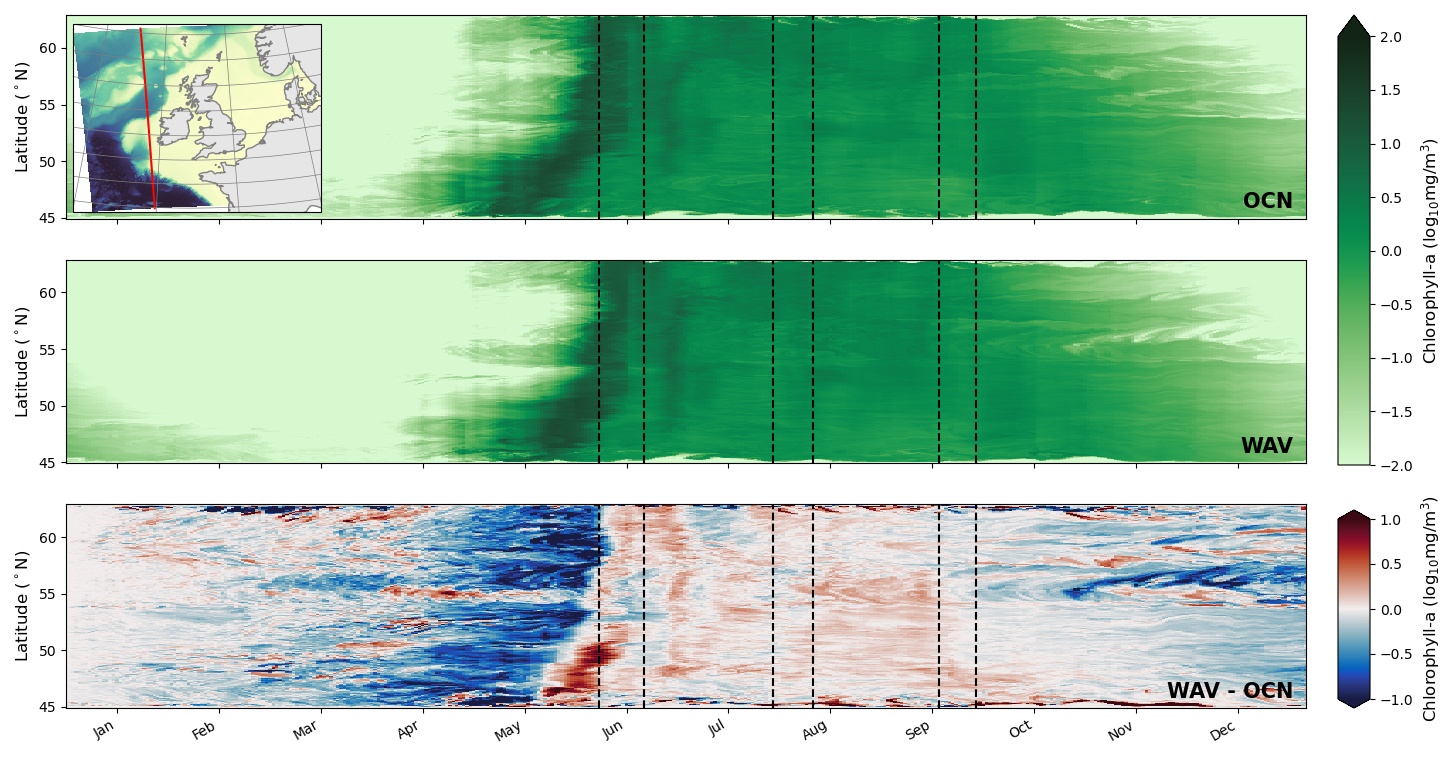
Figure 8 Chlorophyll (averaged over euphotic depth) time/latitude transect along the red line indicated in the top left hand inset for (top) OCN, (middle) WAV, (bottom) WAV-OCN. Black vertical dashed lines show storm periods

4.2 Phytoplankton changes with wave coupling

Figure 8 shows the simulated chlorophyll concentration throughout the year for a transect in the off-shelf region running N–S. Chlorophyll fields are averaged down to the euphotic zone, the depth at which light is 1 % of its surface value, in order to capture sub-surface chlorophyll maximums.

In both the OCN and WAV simulations the bloom originates in the warmer, southern part of the domain with a strong signal around April followed by a period of elevated concentrations that eventually die out in January. In the northern part of the domain the initial bloom occurs approximately two weeks later, with the elevated concentration period ending by November. The bloom is interrupted by storm Hector mid-June and a secondary bloom is clear on the on-shelf part of the transect (48–55° N) at the start of July, which corresponds to the start of the marine heatwave (Fig. 3), two weeks after storm Hector. The WAV simulations additionally show increased chlorophyll concentration in the secondary late June peak, and then in August and September near the shelf break between 48 and 55° N.

By considering the on-shelf, shelf-break and off-shelf regions, as highlighted in Fig. 1, the temporal patterns for the different zones can be assessed. Figure 9 shows the difference in mean net primary production (NPP) as a time-series. The shallow, sheltered on-shelf region is relatively less affected by the addition of waves into the system, whereas the shelf-break and off-shelf zones have a more pronounced difference. In both these regions there is a negative peak followed by a positive one, highlighting the offset nature of the blooms. In the shelf-break region, after the initial blooms for both models NPP levels are consistently higher throughout the summer when waves are included. In off-shelf areas, the offset is greater leading to a larger overall difference in primary production.

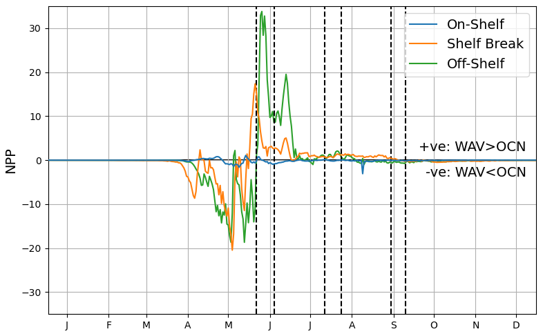
Figure 9 Mean difference in NPP between simulations for off-shelf, shelf-break and on-shelf regions as defined in Fig. 1, with storm periods indicated by black vertical dashed lines.

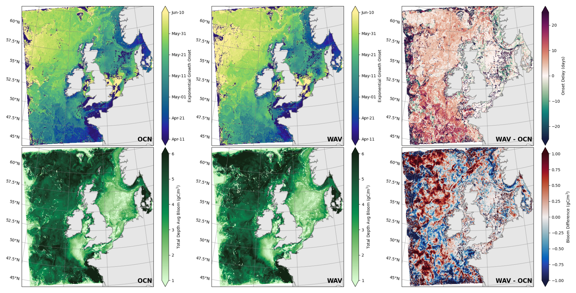
Figure 10 Date of onset of exponential growth (top) and total NPP over the year averaged to the euphotic depth (bottom) for OCN (left), WAV (middle) and the difference; WAV minus OCN (right).

4.3 Bloom phenology

Accurately determining the phenology of phytoplankton blooms is challenging, with different methods yielding wildly different results (Brody et al., 2013). Here we used the approach of Jardine et al. (2022) to predict the bloom onset, with the timing defined as the start of exponential growth in the concentration of chlorophyll (used as a proxy for phytoplankton biomass). This is defined to be the time when the change in the concentration of chlorophyll exceeds 0.15 $\mathrm{mg}{\mathrm{m}}^{-\mathrm{2}}{\mathrm{d}}^{-\mathrm{1}}$ consistently for 5 consecutive days. This approach performs best with full temporal data coverage, making it ideal to apply to model output but not so useful for patchy satellite data.

By applying this algorithm to both model runs, we see that coupling with waves delays the bloom onset across most of the model domain (Fig. 10). On-shelf, the response to wave coupling is minimal as the shallow waters are already well mixed by tidal processes, whereas off-shelf bloom onset is typically 1–2 weeks later with larger delays in the south. Across the entire domain there is a mean delay of 3.2 d.

In addition to delaying bloom onset, the yearly total of chlorophyll averaged over the euphotic depth is up to 20 % higher in the high-productivity region along the northern reaches of the shelf break and also in some deeper waters (Fig. 10).

The date of bloom onset in the model runs is later than observations usually suggest. Later model predictions of bloom onset relative to observations have been observed in past NEMO-ERSEM simulations (Skákala et al., 2020) and, in part, stem from the parametrisation of photosynthesis, phytoplankton growth and grazing effects. The biological model is also influenced by biases in the physical model, including temperature, which directly impacts biological rates as well as the timing of stratification; and the ability to accurately represent optically active components, such as coloured dissolved organic matter (cDOM) and suspended particulate matter (SPM), which impact light attenuation. Nevertheless, spatial variability is captured by the model, such as pockets of very late bloom over the shelf; and the later bloom onset along the shelf break north of Scotland and in the open ocean around 51° N.

5 Wave coupling mechanisms

In this section, we assess the differences in physics and biogeochemistry between the two model simulations to understand the mechanisms behind the differences seen in Sect. 4. By running the same physics and biogeochemical model setup with and without wave coupling, we can isolate the effect of wave coupling, independent of the biases in the models relative to observations.

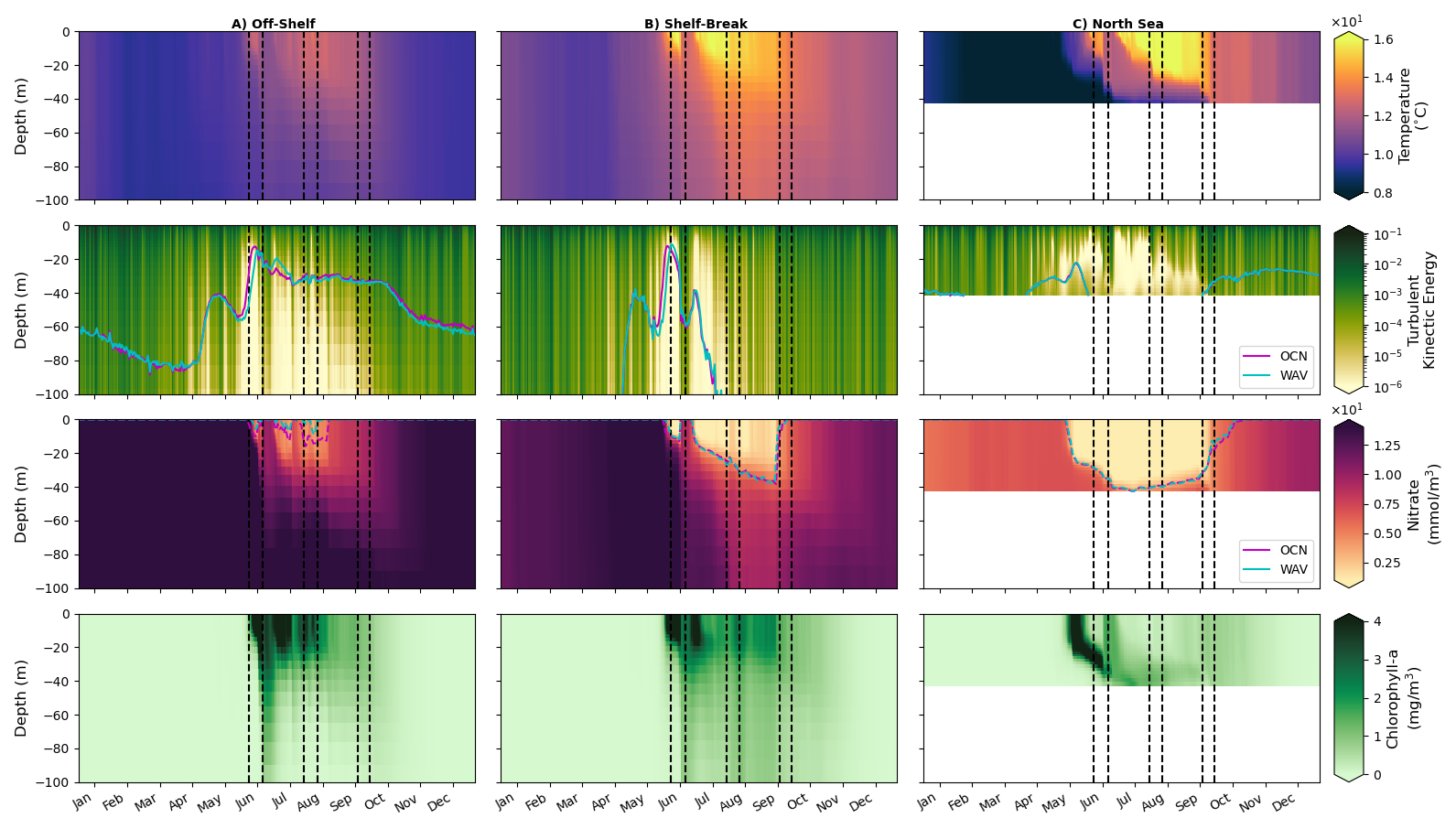
Figure 11 Hovmöller plots (depth/time) of WAV output for potential temperature, turbulent kinetic energy, nitrate, chlorophyll and light availability for (left) off-shelf, (middle) shelf-break and (right) on-shelf North Sea regions defined in Fig. 1. Dashed lines indicate storm periods. The magenta (OCN) and cyan (WAV) time series show euphotic depth (1 % of surface light) in the second row and nutricline depth (3 µmol kg⁻¹ threshold) in the third.

5.1 Physical changes with wave coupling

Figures 11 and 12 show average Hovmöller plots for three distinct regions of the domain; off-shelf, the shelf break and North sea on-shelf region, as defined in Fig. 1. The first (Fig. 11) shows absolute values from the coupled WAV simulation, whilst the second (Fig. 12) shows the difference between the WAV and OCN simulations.

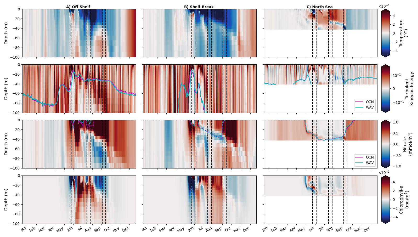
Figure 12 Hovmöller plots (depth/time) of WAV-OCN for potential temperature, turbulent kinetic energy, nitrate, chlorophyll and light availability for (left) off-shelf, (middle) shelf-break and (right) on-shelf North Sea regions defined in Fig. 1. Magenta (OCN)/Cyan (WAV) time series show euphotic depth (1 % of surface light) in the second row and nutricline (3 µmol kg⁻¹ threshold) in the third.

The top row in Figs. 11 and 12 show temperature: when the water column is stratified, the ocean-wave coupled system is cooler in the mixed layer, and warmer below the mixed layer in May–June, before the first summer storm, due to increased vertical mixing when treating waves explicitly. Over the shelf region, this signal is also clear at the start of stratification episodes (May and July), but then reverses after strong mixing events. This difference between the runs when stratified is similar to the results seen in Lewis et al. (2019), however in those experiments the stratification remained for the whole season as there were no disruptions by summer storms in their year of study (2017). These mixing events in 2018; (storm Hector (13 and 14 June), unnamed storm (29 July), storms Ali and Bronagh (18–21 September)) are clearly seen through a sudden erosion of stratification in Fig. 11. Vertical mixing is increased when coupled with waves (2nd row, Fig. 12), and the coupled simulations are generally cooler from the surface down to 60–100 m in the off-shelf and shelf-break regions after storms (3rd row, Fig. 12). This persists even after stratification has re-formed (end June–July) due to a deeper mixed layer in the coupled runs.

The main direct effect of coupling with waves off-shelf and in the shelf-break is to increase turbulent kinetic energy (TKE) in the ocean, which is related to the change in surface roughness and water-side stress, now calculated by the wave model (Figs. 11 and 12, 2nd row). On the shelf break, TKE penetrates deeper in the ocean during summer storms, potentially because of the interaction with the bathymetry and breaking of internal waves. This explains the deeper cooling effect of wave coupling in this region.

On-shelf in the North Sea, the direct effects of wave coupling is more varied, with a decrease in TKE for the main mixing events during the stratification period (Fig. 12, rightmost panels). This is likely due to the fact that wave age in the North Sea tends to be small as waves there are generated by local wind, not remotely generated swells. Therefore in this region, and in the case of intense events like the ones responsible for deep mixing, the waves will tend to extract momentum from the atmosphere before it is passed to the ocean, and therefore reduce TKE (Gentile et al., 2021). This explains the warming with wave coupling after mixing events in this region: the mixing in the ocean has become shallower with wave coupling as waves extract energy from the atmosphere before it is passed to the ocean.

5.2 Linking physical and biogeochemical changes from wave coupling

Nutrient differences with wave coupling are consistent with temperature changes once stratification is established (Figs. 11 and 12, 3rd row). Extra TKE introduced by the wave model brings additional nutrients from nitrate-rich deeper layers to the surface, reducing nutrient content in these deeper layers. Each storm is also clearly seen in the off-shelf and shelf-break profiles, increasing nutrient concentration near the surface, and this effect is stronger with wave coupling. At the onset of stratification (May–June), the pattern in nitrate near the surface is anti-correlated with the pattern of chlorophyll-a content (Fig. 11). This pattern is controlled by the consumption of nitrate by the spring phytoplankton bloom, which occurs later with wave coupling (Fig. 11, 4th row). From late June, chlorophyll-a content under the mixed layer is generally larger when coupled to the wave model, illustrative of a stronger export of phytoplankton to depth with stronger TKE. The additional mixing in these regions results in increased chlorophyll throughout the column (Figs. 11 and 12, 4th row). Increased nutrient concentrations near the surface after mixing events may be offset by reduced light availability due to a deeper mixed layer and enhanced vertical mixing that transports chlorophyll out of the euphotic zone.

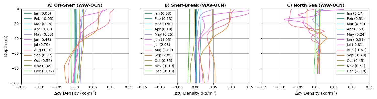
Figure 13 Difference in density (kg m⁻³) stratification profiles in the upper 100 m throughout the year for the three regions. Density given in σ_T ($=\mathit{\sigma }-\mathrm{1000}$) coordinates, with the total difference throughout the column for each month shown in parenthesis.

The delay in phytoplankton bloom with wave coupling can be explained by a combination of the change in light availability and temperature for the phytoplankton at the early stages of the bloom, both of which impact growth rate and are reduced by wave mixing at the time of bloom onset. At the beginning of the summer stratification period, the formation of a shallower mixed layer helps retain phytoplankton in the euphotic zone, allowing phytoplankton to bloom because of high nutrient concentration and light availability. Then, throughout the growing season phytoplankton become limited by nutrient availability and the bloom reduces. Coupling to the wave model consistently reduces stratification in April–May (Fig. 13) by increasing TKE, which decreases temperature and leads to phytoplankton going through deeper cycles in the emergent mixed layer with longer time in regions where light availability is lower. This delays the phytoplankton bloom, which happens 1–2 weeks later with wave model coupling.

On the other hand, the impact of TKE is limited on the shelf even during strong mixing events. By the time storm Hector crosses the domain, phytoplankton have already consumed most of the existing stock of nitrate and there is no nutrient-rich deep layer to resupply. Interestingly, each phytoplankton “bloom” associated with the strong mixing events and termination of marine heatwaves is reduced by wave coupling. In the coupled case, momentum from the atmosphere is used to grow young waves. This delays the transfer of energy from atmosphere to ocean. In the ocean-only simulation, where waves are not explicitly included, the energy can abruptly mix the water column without this intermediate step. The apparent summer/autumn blooms after these events are not necessarily new growth, with increased surface chlorophyll the result of the mixing of the sub-surface chlorophyll maximum up from the nutricline to the surface, giving the appearance of a bloom.

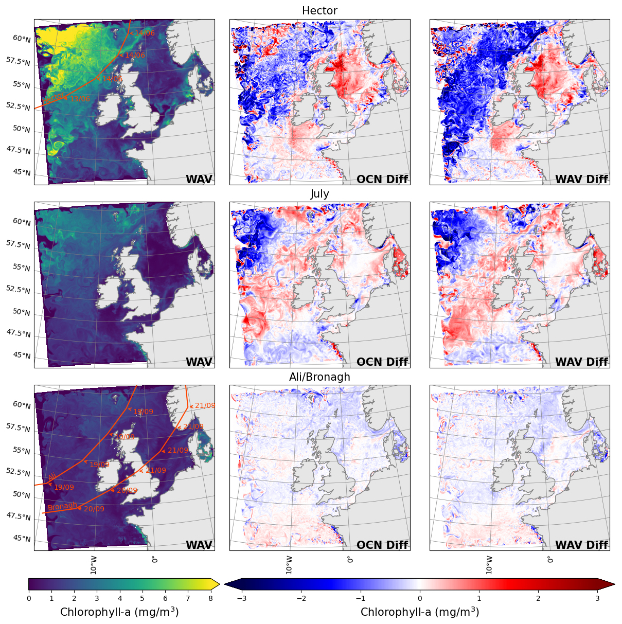
Figure 14 Mean chlorophyll in the five days before the storm from the ocean-biogeochemistry model (left), the difference between the mean of the five days after the storm and the mean of the five days before the storm from the ocean-biogeochemistry model (middle) and the ocean-wave-biogeochemistry model (right), for storm Hector (top), July storm (middle) and storms Ali and Bronagh (bottom). The start of the five days before and the end of the five days after the storms are highlighted in Fig. 3 as vertical bars.

5.3 Storm impact

There is a clear difference in response to storms between the deeper, open ocean and the sheltered shallow on-shelf area of the North Sea. Off-shelf, the phytoplankton sit near the surface so when the storms pass over the region they mix the chlorophyll from 0–20 m down to about 100 m, as seen in Fig. 11, row 4. At the same time nutrients are brought nearer the surface by storm mixing because injected TKE reaches nutrient-rich water below the nutricline (Fig. 11, row 3). The stage of the phytoplankton bloom at which the storm occurs also affects the response. At the time of the second storm, the phytoplankton levels have decreased from the initial bloom, as such the mixing has a similar effect to the first storm, but of a smaller magnitude.

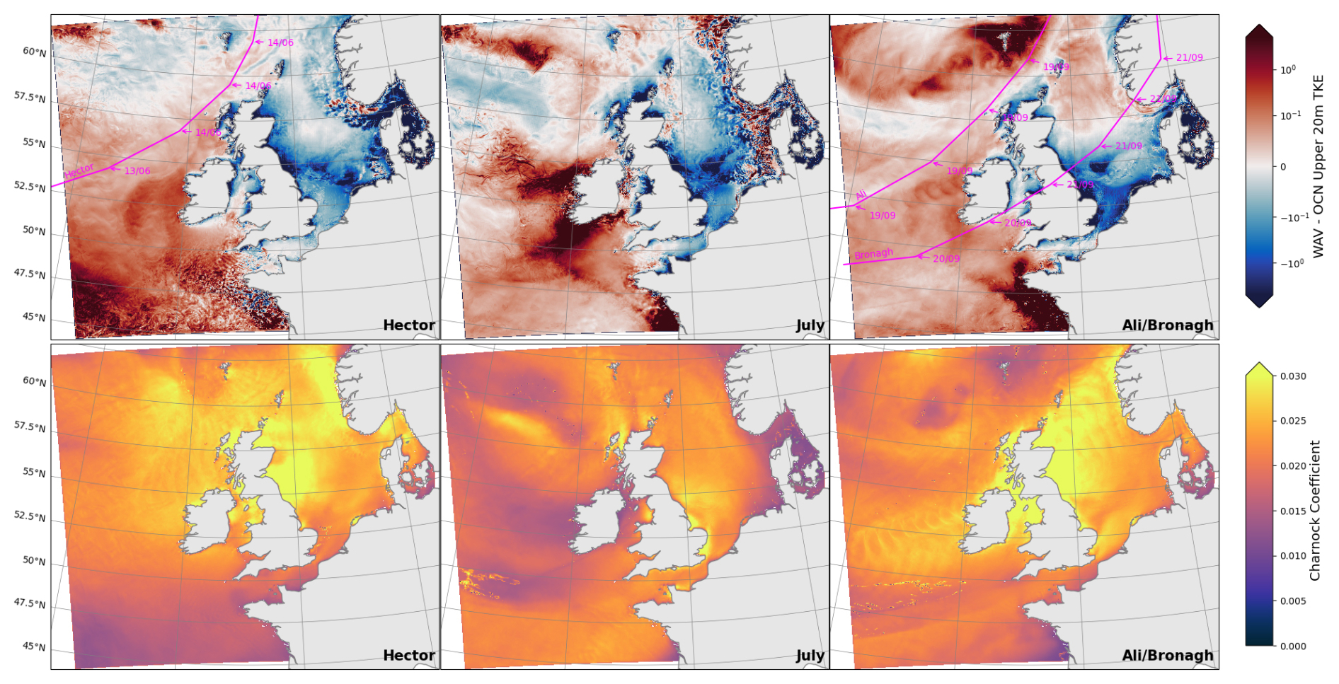
Figure 15 Difference in upper 20 m turbulent kinetic energy (TKE) between simulations (top) and the Charnock coefficient from wave model (bottom) on; 14/6 for storm Hector (left), 29/7 for the July storm (middle) and 20/9 for storms Ali/Bronagh (right). Storm paths are shown in magenta where available.

In contrast, on-shelf the profiles of chlorophyll and nutrients indicate that the bloom starts near the surface and then moves deeper in the water column, where nutrients are still available (Fig. 11). When the first storm occurs the chlorophyll maximum is still at depth, so the mixing spreads the bloom back up through the water column. By the time of the second summer storm in July, nutrients are depleted throughout the column and the phytoplankton bloom has finished, so the storm has a limited impact.

As previously shown in the satellite measurements, the passage of storms across the domain has a large impact on the distribution of chlorophyll (Fig. 4). The results from the models for the same period are shown in Fig. 14. Due to the biases highlighted in Sect. 4.1, the chlorophyll concentrations are generally higher in the models relative to the satellite observations, meaning Storm Hector has a larger impact on sea surface chlorophyll concentrations in the models than it does in the observations. Nevertheless, the spatial pattern of the response to the storm is similar between the models and the observations, with a suppression of phytoplankton activity off-shelf and increased activity on-shelf. For the July storm, the models capture the increase in the concentration of chlorophyll on the western and northern edges of the North Sea (Fig. 14), whilst there is little effect observed in the satellite measurements. For storms Ali and Bronagh, the north–south gradient in the response in the North Sea is well captured by the model, though it is not as intense as the earlier storms.

One element captured by satellite observations but not by either of the models is an autumn bloom in the southern North Sea, that appears to be elevated by the passing of the autumn storms Ali and Bronagh (Fig. 4, row 3). Whilst it is possible that the satellite measurements are not representative, the absence of a bloom in the models is more likely to be due to the biogeochemical model not encountering the right physical conditions. The issue could be related to the temperature bias, or due to feedback mechanisms between the waves and atmosphere that are not represented by the models, such as the change in surface roughness due to young waves.

The difference in TKE between the model simulations as a result of the storms is shown in Fig. 15. The dominant impact of wave coupling is an increase in mixing energy across the western half of the domain where the storms originate, whereas east of the British Isles in the sheltered areas of the North sea, especially the south, there is a reduction in TKE due to the wave coupling.

Also shown in Fig. 15 is the Charnock coefficient, a parameter that relates the sea surface roughness to wind friction velocity. A high Charnock value is associated with young waves and high wind speed (Moon et al., 2004). In the WAV simulation the Charnock coefficient and TKE are correlated, with temporal Pearson correlation values in excess of 0.6 across the domain.

In the wave coupled system, the high Charnock value in the North sea during storms is due to a large proportion of the wind stress energy being used to create growing waves, whereas in the parameterised OCN simulation the wind stress energy is instead transferred directly into the ocean. The difference in energy transfer results in the differences in TKE seen in Fig. 15, but the impact on phytoplankton in the North sea is minimal as the region is shallow and already well mixed by tidal processes.

6 Conclusion

This paper is the first use of a km scale coupled wave-hydrodynamic-ecosystem model. Whilst simulations suffered from a systematic warm bias, the results supports similar findings to the studies of Liu et al. (2025) and Tensubam et al. (2024). The biases make commentating on the scale of the impact challenging, however the use of a twin study isolates the mechanistic impact of waves on shelf-seas ecosystems which allows an investigation into the drivers behind how seasonal productivity can be altered by the sea state.

The study identified regional and seasonal variations in the response of phytoplankton to wave activity: during the bloom (in March–April in the observations, April–June in the model), with enhanced wave activity off-shelf or near the shelf break inducing mixing of the surface bloom down into deeper waters, and the chlorophyll concentration near the surface is reduced. On-shelf, enhanced wave activity tends to generally increase chlorophyll activity near the surface from July–September, likely because light is available throughout the water column, and wave mixing helps mix nutrients from rich to poor regions. This could either occur through advection of nutrient-rich river plumes or through vertical mixing if the injection of TKE is deep enough and nutrients are still available near the bottom of the sea, which is possibly not the case in May–June (Fig. 2).

This paper also investigated the effects of explicitly treating wave input to the ocean as a separate model coupled to the ocean with a 1.5 km grid spacing. The main findings depend on the region of interest:

• Off-shelf on the Atlantic side of the domain, explicit coupling with waves increases the injection of turbulent kinetic energy into the ocean across depth (Fig. 12). This reduces stratification at the start of the growing season, meaning that phytoplankton is not trapped as close to the surface, and gets less light through deeper mixing cycles induced by stronger TKE. The bloom is therefore triggered later with the wave model (Fig. 10). Total chlorophyll concentration and NPP are increased in summer, as stronger TKE injection leads to more intense phytoplankton secondary blooms

• At the shelf-break the conclusions are similar to off-shelf, with an increase in summer production. This increase is less pronounced than off-shelf due to the transition into shallower well mixed region.

• On-shelf, the changes are smaller for several reasons; Firstly outside the bloom season the euphotic depth is close to the actual shelf depth in the North Sea, so additional mixing does not affect the phytoplankton bloom as much. Second, the North Sea is sheltered by the British Isles and has younger waves than the Atlantic side. Young waves extract momentum from the atmosphere before passing it to the ocean, and delay the transfer of TKE in the ocean. This is visible during summer storms (Fig. 15), when marine heatwave stratification breaks. In the WAV case, the waves delay transfer of momentum and spread the event over a longer time acting to “flatten the curve”. Thus the mixing event is less sharp and intense, and the elevated chlorophyll concentrations less peaked.

Future work will include fixing the temperature bias from the surface forcing and evaluating a fully coupled simulation which includes a regional configuration of the Met Office atmosphere and land system: the physics-only configuration for which is documented in a companion paper (Berthou et al., 2026). In the present work, the ecosystem model does not feedback to the physical system: future work will include chlorophyll feedback on light penetration in the physical ocean building on Skákala et al. (2020), and providing surface chlorophyll values to the atmosphere for the calculation of surface albedo. Rivers will also be coupled to the ocean, with the target of enabling variable nutrient loads to enter the ocean through the river instead of the current climatological input.

A fully coupled system will enable the study of compound events across land and marine environments in a changing climate. Representing the ocean colour feedback on the ocean and atmosphere was indeed recently shown to be important for climate projections in the Mediterranean, with resulting SST changes up to 1°C (Zhang et al., 2025).