Three-dimensional structure of sub-mesoscale eddies on the continental shelf

Sub-mesoscale eddies are oceanic features crucial for energy transfer processes, transport of heat and biogeochemical tracers, and for promoting diversity in marine ecosystems. Their relatively small length scales (< 20 km) and short lifespans ∼ O(days), make their characterization challenging using field measurements. In this paper, we combined remote sensing, ocean glider, High-Frequency Radar, shipborne, and mooring data to investigate the internal structure and dynamical properties of sub-mesoscale eddies and peddies (“petite” eddies; D ≤ 10 km extending through the water column) along the Wadjemup (Rottnest) Continental Shelf (WCS), Western Australia. Data collected in August 2010 showed an anti-cyclonic (counterclockwise) mesoscale eddy spawning several cyclonic (clockwise), cold core sub-mesoscale eddies that promoted upwelling (vertical extension of 185 m) with maxima in chlorophyll concentration at the centre. Results suggested that sub-mesoscale eddies drive chlorophyll advection either at (in) their periphery (centre) of cyclonic (anti-cyclonic) eddies, or at their interfaces. In general, cyclonic eddies promoted upwelling and anti-cyclonic eddies promoted downwelling; however, our data also showed that upwelling conditions could also occur in anti-cyclonic eddies. Winds were found to affect the internal structure and lifecycle of sub-mesoscale eddies, particularly under strong wind (speeds > 7 m s⁻¹) conditions, through upwelling and/or vertical mixing. In the presence of dense shelf water outflows along the continental shelf, sub-mesoscale eddies were found to trap, upwell, and transport denser nearshore waters off the continental shelf. This unique dataset provided a detailed picture of the three-dimensional structure of sub-mesoscale eddies, including the characterization of sub-surface eddies, and contributes to the understanding of their role in chlorophyll advection in shelf and coastal environments.

1 Introduction

Mesoscale and sub-mesoscale features are ubiquitous in the world's oceans, acting as reservoirs and pathways of 90 % of the ocean's kinetic energy (Capet et al., 2008; Chelton et al., 2007; Ferrari and Wunsch, 2009; Fu et al., 2009). They are crucial for maintaining energy balance across scales (Chen et al., 2023) and transporting heat, momentum, mass, and biogeochemical tracers in the oceans, also promoting biodiversity in marine ecosystems (Damien et al., 2023; Lévy et al., 2018; Mahadevan, 2016). In continental shelf regions, these processes also facilitate exchanges between offshore and coastal waters. Through cross-shore transport, they contribute to carbon export and the fate of particulate organic carbon and biogeochemical budgets (Mahadevan, 2016) with important implications for plankton, fisheries, and fisheries management (Akpinar et al., 2020, 2022; Guerrero et al., 2020; Irigoien et al., 2007). Sub-mesoscale eddies contribute to nutrient cycling, primary production, structure and functioning of phytoplankton ecosystems in coastal areas (Fig. 1a; Lévy et al., 2001; Davila et al., 2021; Mahadevan and Tandon, 2006; Oguz et al., 2015; Veatch et al., 2024).

These features occur in the transition between mesoscale dynamics and small-scale turbulence (Thomas et al., 2008; Kubryakov et al., 2022). Sub-mesoscale processes are typically characterised by horizontal scales of order 1–20 km, although their spatial extent is not universal and depends strongly on the local Rossby deformation radius and stratification. Their temporal scales generally range from hours to a few days. Their strong ageostrophic nature can lead to Rossby numbers ∼ O(1) or larger and induce high vertical velocities in their core (10–100 m D; Lévy et al., 2012; McWilliams, 2016; Thomas et al., 2008; Zatsepin et al., 2019).

Consequently, they can lead to intense localised mixing (McWilliams, 2016; Thomas et al., 2008) and vertical transport of nutrients and suspended matter (Rubio et al., 2018; Su et al., 2021; Zhang and Qiu, 2020), driving phytoplankton growth and enhancing primary productivity or reducing biological production in the euphotic zone through advection, upwelling or downwelling (Davila et al., 2021; Lévy et al., 2012; Mahadevan and Tandon, 2016; Thomas et al., 2008).

Understanding the impacts of small and short-lived features on ecosystems is crucial but limited due to technical challenges, such as the availability of data with sufficient spatial and temporal resolution (Liu et al., 2015; Parks et al., 2009; Zhang et al., 2019). Remote sensing observations stand out as powerful tools for detecting and tracking sub-mesoscale features (e.g., Bitencourt et al., 2025; Cosoli et al., 2020; Lipinskaya et al., 2023; Zatsepin et al., 2019). However, the data is limited to the surface and insufficient for characterising their internal structure. More conventional in situ measurements offer detailed, high-resolution vertical profiles that can help to resolve internal dynamics; however, not with sufficient resolution. Thus, a combination of datasets (e.g., vessels, moorings, ocean gliders, autonomous underwater vehicles, satellite) can provide a detailed picture of the three-dimensional structure of eddies and their evolution in coastal, shelf and offshore environments (e.g., Bouffard et al., 2012; Bosse et al., 2017; Fayman et al., 2019; Veatch et al., 2024).

The Wadjemup (Rottnest) Continental Shelf (WCS), a microtidal and oligotrophic marine environment located on the south-west coast of Australia, is a region rich in sub-mesoscale eddies (Fig. 1a; Bitencourt et al., 2025; Cosoli et al., 2020; Kendrick et al., 2023; Pattiaratchi and Eliot, 2009). In this region, the Australian Integrated Marine Observing System (IMOS) has been collecting data from different platforms for over a decade and enabled the characterisation of small-to-large scale features (e.g., Bitencourt et al., 2024, 2025; Cosoli et al., 2020; Kodithuwakku 2024; Pattiaratchi et al., 2017).

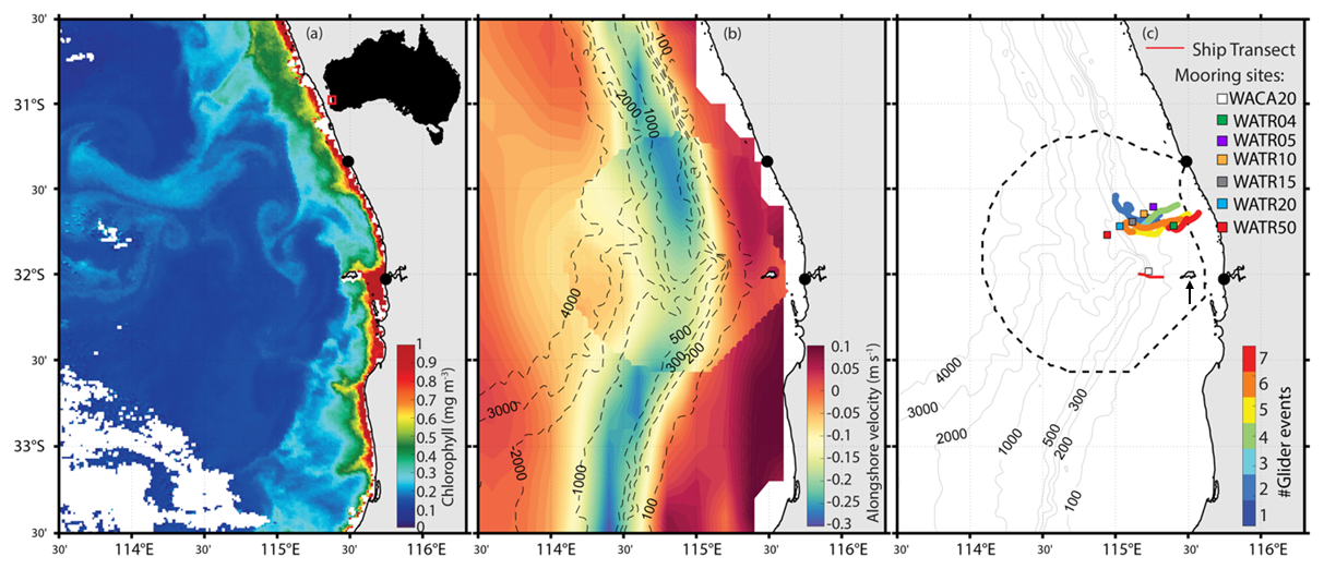
Figure 1 (a) Remotely sensed chlorophyll a on 28 March 2016, (b) long-term (2010–2018) averaged alongshore velocities from altimetry and HFR observations in Wadjemup Continental Shelf; and (c) HFR domain (dashed line), glider (coloured lines) and ship (red line) tracking, and mooring locations (coloured squares). Bathymetric contours (in metres) are shown in (b) and (c). Black dots at the shoreline in (a), (b) and (c) represent HFR shore stations. The upward arrow in (c) points to Rottnest Island the location of the wind records.

Complex circulation patterns across multiple scales characterise the WCS area, such as an anomalous poleward eastern boundary current, micro-tidal regime, wind-driven coastal circulation, sub- to meso-scale eddies, complex bathymetric features with a canyon reaching as deep as 4000 m, and circulation responses to remote forcing associated with the Leeuwin Current system and coastally trapped waves (Trotter et al., 2019). Wind forcing is amongst the strongest globally and drives the circulation along the shelf (Bitencourt et al., 2024; Mihanović et al., 2016), particularly under the summer land-sea breeze regime (maximum daily wind speeds frequently exceeding 15 m s⁻¹) and winter storms (speeds > 30 m s⁻¹; Pattiaratchi et al., 1997; Rafiq et al., 2020; Verspecht and Pattiaratchi, 2010; Zaker et al., 2007). Strong inertial-diurnal resonance also occurs in the region due to its proximity to the critical latitude (30° S) (Mihanović et al., 2016; Rafiq et al., 2020). In addition, strong air-sea heat fluxes and low river outflows along the coast contribute to dense shelf water transport which is then transported offshore as gravity currents (Mahjabin et al., 2019a, b; Pattiaratchi et al., 2011; van der Mheen et al., 2024).

The Leeuwin Current (LC), Capes Current (CC), wind forcing, their interactions and deeper water dynamics control the circulation along the South-west Australian coast (Pattiaratchi and Woo, 2009; Pattiaratchi and Buchan, 1991). The LC is a warm, relatively shallow (< 300 m depth) and narrow (∼ 100 km width) eastern boundary current that flows poleward against the prevailing equatorward winds favouring downwelling along the shelf break towards the South Australian coast (Feng et al., 2009; Pattiaratchi and Woo, 2009; Pearce and Pattiaratchi, 1999; Wijeratne et al., 2018). Thus, the LC, that inhibits large-scale upwelling, contrasts with the equatorward-flowing upwelling-favourable currents typically found along the eastern boundaries of ocean basins. In contrast, the CC is a seasonal inner-shelf wind-driven equatorward-flowing current that promotes weak, shallow (< 50 m) upwelling of more saline and colder water (21–24 °C) inshore of LC (Bitencourt et al., 2024; Gersbach et al., 1999; Pattiaratchi and Woo, 2009; Pearce and Pattiaratchi, 1999).

Local and large-scale wind patterns favour, reinforce or weaken the poleward-flowing LC and the seasonal wind-driven equatorward-flowing CC (Fig. 1b). Under prevailing southerly winds in the warmer months, CC flows equatorward along the inner shelf, whilst the LC weakens and is displaced offshore (Bitencourt et al., 2024; Gersbach et al., 1999; Pearce and Pattiaratchi, 1999). Under weaker southerly or variable winds, particularly over cooler months, CC is absent whilst the LC is strongest along the shelf (Bitencourt et al., 2024; Cresswell, 1996; Pattiaratchi and Woo, 2009; Wijeratne et al., 2018).

Mesoscale and sub-mesoscale eddies are ubiquitous features in the region, particularly along the interfaces of the LC (Bitencourt et al., 2024, 2025; He et al., 2021; Kodithuwakku, 2024; Rennie et al., 2007). They spawn along the LC path, particularly through interactions with coastal and bottom topography (changes in coastline orientation, bathymetric features; Cosoli et al., 2020; Kodithuwakku, 2024; Rennie et al., 2007; Waite et al., 2007), barotropic instabilities and interactions with the CC and offshore mesoscale eddies (Bitencourt et al., 2024, 2025; Pattiaratchi and Mihanović, 2014). Peddies are defined as sub-mesoscale eddies that form in shallow coastal waters, typically in water depths < 200 m and occupy the majority of the water column. They have typical eddy D < 10 km and lifespans of 1–2 d. They are generated in regions of strong horizonal flow shear and influenced by bottom topography and friction because their vertical extent often spans much of the water column. Sub-mesoscale eddies and peddies are difficult to observe and characterize due to their small spatial and temporal scales, with limitations in both observational capabilities and modelling resolution hindering a complete understanding of their internal structure and variability under different forcing condition (Bitencourt et al., 2025; Cosoli et al., 2020; Pattiaratchi and Mihanović, 2014).

In this paper, we use a multi-platform approach to investigate the internal structure of sub-mesoscale eddies (< 20 km D) and peddies (i.e., “petite” eddies; D ≤ 10 km extending through the water column) along the Wadjemup (Rottnest) Continental Shelf. In particular, we aim to: (1) characterize their physical and biogeochemical structure and determine whether these features display consistent signatures across observations; and (2) evaluate how these eddies influence chlorophyll distribution on the shelf.

2 Data and Methods

The Australian Integrated Marine Observing System (IMOS) was established in 2006 and this study used data acquired as part of IMOS in Western Australia (WAIMOS) using a variety of data collecting platforms including research vessels, oceanographic mooring time series, ocean gliders, surface currents using High Frequency Radar, satellite remote sensing and meteorological data.

2.1 R/V Southern Surveyor

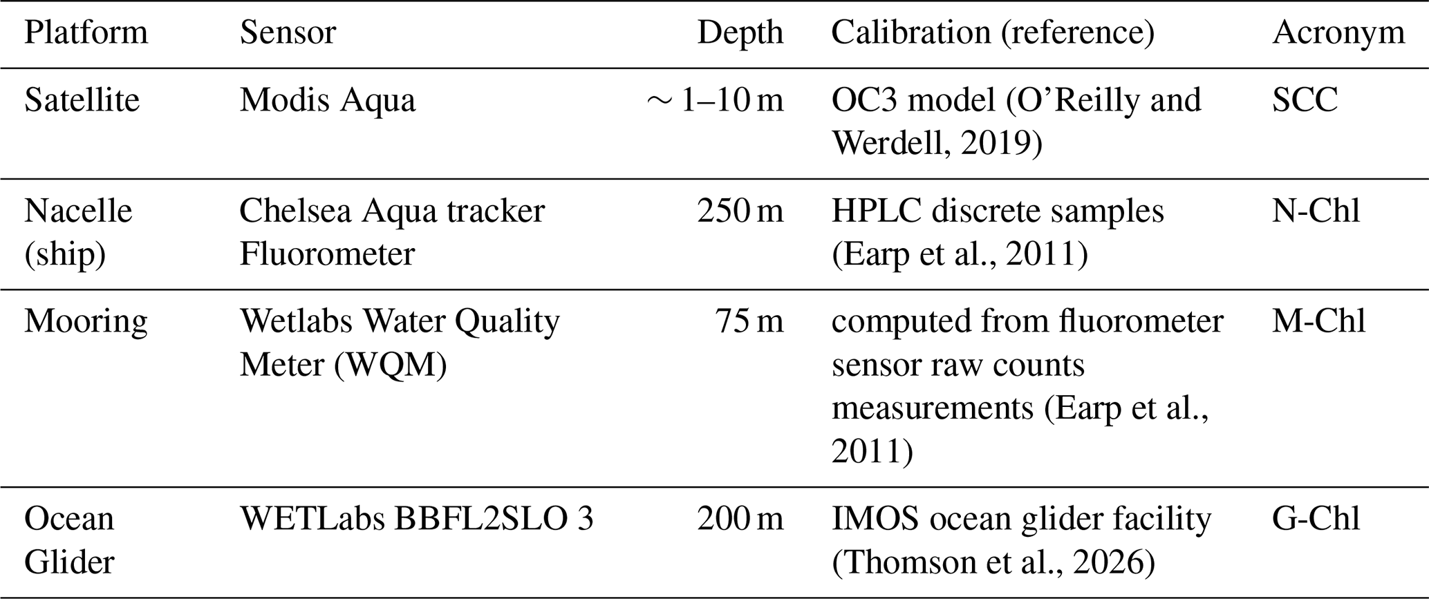
The R/V Southern Surveyor research cruise (SS2010_v06) collected hydrographic and biological data between 29 July to 9 August 2010, with the aim of investigating the slope and shelf processes along the south-west region of Western Australia in winter (Pattiaratchi and Hanson, 2010). Data collected included that from a towed platform Nacelle with profiles from the surface to a maximum depth of 200 m in a yo-yo mode at a vertical resolution of 1 m. The horizontal spacing of each dive varied within 1–4 km, depending on the velocity of the ship. Sensors on Nacelle included a Seabird SBE911 CTD, a SBE43 oxygen sensor, a Chelsea Aqua tracker Fluorometer (N-Chl, Table 1), and a Wetlabs C-Star™ transmissometer. Sensor calibrations were undertaken using bottle samples (Pattiaratchi and Hanson, 2010).

Table 1 Summary of chlorophyll measurements.

Current profiles were collected using a hull-mounted, 75 kHz RDI Acoustic Doppler Current Profiling (ADCP), collecting subsurface current data at a 10 min ensemble time and a vertical resolution of 16 m. Data were collected by the Commonwealth Scientific and Industrial Research Organisation (CSIRO). A transect (Fig. 1c) showed the presence of a peddie on 3 August 2010, west of Rottnest Island.

2.2 Moorings

Subsurface currents, temperature, salinity, chlorophyll fluorescence (M-Chl) data were collected across several mooring locations within the WCS (Fig. 1c). Moorings were located between 45–65 km offshore, at nominal water depths of 40, 50, 100, 150, 200 and 500 m (mooring codes: WATR04, WATR05, WATR10, WATR15, WATR20 and WATR50, respectively), and in the Perth Canyon (WACA20) at a depth of ∼ 200 m (Feng et al., 2025). They were equipped multiparameter probes with SBE39 and SBE39plus sensors from SeaBird Electronics and RBR XR420-CTD from RBR. Bottom-mounted, upward-looking acoustic 190 kHz Doppler current meter from Nortek Continental measured horizontal and vertical currents along the water column (see Mihanović et al., 2016; Mahjabin et al., 2019b). At the WACA20 mooring site (Fig. 1c), a Wetlabs Water Quality Meter (WQM) was deployed at 75 m water depth that measured, temperature, salinity and chlorophyll fluorescence (M-Chl, Table 1). Further information regarding data processing and quality control procedures in WCS-IMOS mooring data refer to Morello et al. (2014) and Bui and Feng (2025).

2.3 Ocean gliders

High-resolution sub-surface measurements of salinity, temperature, dissolved oxygen (DO) and chlorophyll fluorescence (G-Chl, Table 1) were collected using Teledyne Webb Research Slocum electric G2 gliders sampling to a maximum 200 m water depth. Each glider was equipped with a pumped SeaBird Scientific CTD sensor, WETLabs BBFL2SLO 3 parameter optical sensor (Chlorophyll fluorescence G-Chl, coloured dissolved organic matter, and 660 nm backscatter), and an Aanderaa Oxygen optode (Pattiaratchi et al., 2017; Mahjabin et al., 2019b). The glider collected science data (CTD_bio-optics) between the surface to a maximum 200 m depth with a mean travel speed of ∼ 25 km D (Pattiaratchi et al., 2011). Data sampling rate was set at 4 Hz, resulting in measurements with approximately 7 cm vertical resolution. The gliders were programmed to surface every 2 h and transmit its position and send a subset of science data to the shore station. Over this 2 h period the glider traversed 1–2 km, performing 5–10 vertical dives, resulting in the lateral spacing of profiles between 100–250 m in 50 and 200 m water depths, respectively. Data were post-processed after recovery with QA/QC procedures as described in Woo (2021). The science data were processed using the IMOS ocean glider analysis software Gliderscope in MATLAB (Hanson et al., 2017). The data were linearly interpolated into bins of 0.2 m vertically and 4.3 min in time into a 1000 × 1000 grid using Gliderscope (Hanson et al., 2017). The calibration in temperature and salinity measurements achieved an accuracy of ±0.002 °C and ±0.01, respectively (Chen et al., 2019). All the sensors on the gliders were returned to the manufacturer for calibration annually. This included the CTD, DO Optode and the Ecopuck (Thomson et al., 2026). Depth-averaged current (DAC) from the Slocum glider was estimated as the difference between GPS-derived displacement over a dive cycle and the glider's dead-reckoned displacement based on its hydrodynamic flight model, divided by the elapsed time (Rudnick et al., 2015). These techniques are included in the routines provided by the manufacture. There was no vertical averaging (they are depth mean currents) or smoothing applied (have a value every surfacing in our case every 2 h). The quality control was only to check the values of derived velocities are within an acceptable range. The glider derived DAC speeds were within the range 0 < DAC < 0.55 m s⁻¹.

For our analysis, we selected events from seven different glider missions (Fig. 1c; Table 2): (1) 3–4 August 2010; (2) 16–18 August 2010; (3) 16 February 2014; (4) 23 February 2014; (5) 26–27 May 2015; (6) 28–30 May 2015; and (7) 1–2 June 2015.

2.4 High-Frequency Radar

High-resolution (4 × 4 km; 1 h) surface current fields (top ∼ 1.5 m layer) were collected with a pair of WEllen Radar (WERA) phased-array High-Frequency Radar (HFR) shore-based stations (Fig. 1c) located at Guilderton (GUI) and Fremantle (FRE). In this study, we used quality-controlled, delayed-mode, 2 × 2 km interpolated gridded, 33 h low-pass filtered, hourly and daily averaged surface current data (Bitencourt et al., 2024; Cosoli and Grcic, 2024) during selected events identified from the ocean glider data between 2010–2015 (see above and Table 2). Full descriptions of the instrumentation, specifications used in the WCS – HFR system and quality control tests are provided in Mihanović et al. (2016), Bitencourt et al. (2024, 2025), Cosoli and Grcic (2024) and Cosoli et al. (2020).

2.5 Ocean colour data

Level 3 daily sea surface chlorophyll concentration data (SCC, 1 km resolution, Table 1) and Sea Surface Temperature skin (SST, ∼ 2 km resolution) were available from MODIS Aqua and Advanced Very High-Resolution Radiometer (AVHRR) and were accessed through IMOS (Govekar et al., 2022).

2.6 Wind data

Hourly wind speed and direction at Rottnest Island weather station (located ∼ 25 km offshore from the coast, 43 m elevation, Fig. 1c) were obtained from the Bureau of Meteorology (BOM). Wind speeds were converted to the standard 10 m reference height (van der Mheen et al., 2020).

2.7 Analysis techniques

To characterize the vertical structure and dynamical properties of submesoscale eddies and peddies, we estimated relative vorticity and Rossby number using velocity measurements from different observational platforms. Our main objective was not to derive a complete two-dimensional vorticity field, but rather to obtain an order-of-magnitude estimate of the Rossby number (i.e., whether Ro was O(0.1), O(1), or larger) in order to assess whether the observed structures were consistent with sub-mesoscale dynamics. Because the available observations differed substantially in their spatial sampling, different methodological approaches and approximations were required for each dataset, particularly for the glider and shipborne measurements where only partial velocity information was available.

In the following equations, u and v represent the zonal and meridional velocity components of ocean currents, respectively. U is the velocity component perpendicular to the glider track, s is the distance along the perpendicular glider track, and ζ is the relative vorticity. The Coriolis parameter is defined as f = 2Ωsinθ, where $\mathrm{\Omega }=\mathrm{2}\mathit{\pi }/\mathrm{86}\mathrm{400}$ rad s⁻¹ is the Earth's rotation rate and θ is the latitude.

For the HFR observations, the availability of gridded two-dimensional surface velocity fields allowed the direct calculation of relative vorticity as $\mathit{\zeta }=\frac{\partial v}{\partial x}-\frac{\partial u}{\partial y}$, using a central finite-difference scheme (Bitencourt et al., 2025; Cosoli et al., 2020). The Rossby number was then estimated as Ro$=\frac{\mathit{\zeta }}{\left|f\right|}$.

The moored ADCP observations were mainly used to investigate the temporal variability and vertical structure of the observed features, rather than to estimate horizontal vorticity, since the fixed-point measurements do not resolve horizontal velocity gradients.

For the glider and shipborne ADCP observations, the spatial sampling did not allow reconstruction of the full two-dimensional velocity field. Therefore, relative vorticity could not be directly estimated in a dynamically rigorous sense (e.g., from cylindrical eddy geometry and azimuthal velocity structure). Instead, we used along-track horizontal shear as a proxy to obtain an order-of-magnitude estimate of Rossby number following Rossi et al. (2013).

Depending on the orientation of the transect relative to the observed structure, either the zonal shear component $\left(\partial v/\partial x\right)$ or the meridional shear component $\left(-\partial u/\partial y\right)$ was estimated. For the glider observations, the Rossby number proxy was calculated as Ro$=\frac{\partial U/\partial s}{\left|f\right|}$. For the shipborne ADCP observations collected on 3 August 2010 (Fig. 1c), we applied the zonal shear approximation Ro$=\frac{\partial v/\partial x}{\left|f\right|}$ was applied due to the predominantly east–west orientation of the ship transect.

Because these estimates rely on a single velocity component, they likely underestimate the magnitude of the full relative vorticity field. However, assuming approximate rotational symmetry of the observed structures, the along-track shear measurements still provide a useful qualitative estimate of circulation strength and Rossby number. Their primary purpose is to assess whether the observed structures exhibit Rossby numbers of order unity, consistent with submesoscale dynamics.

Different approaches were also used to estimate the horizontal dimensions of the sub-mesoscale eddies and peddies. For the gridded HFR data, an eddy-detection algorithm (Nencioli et al., 2010) was applied to extract ellipse characteristics, including the major and minor axes and eccentricity (see Bitencourt et al., 2025; Cosoli et al., 2020). For the glider observations, two methods were applied on a case-by-case basis: (1) fitting an ellipse to looping glider trajectories in cases where the platform appeared temporarily trapped and advected within the eddy core, providing an approximate estimate of the horizontal scale of the structure, and (2) defining the horizontal extent of the surface temperature anomaly.

2.8 Chlorophyll measurements

The study area is an oligotrophic region, with low chlorophyll concentration (< 1 mg m⁻³; Chen et al., 2019). Chlorophyll was measured using multiple observational platforms and sensors, including satellite remote sensing (SCC) and in situ chlorophyll fluorescence (Table 1). This study focuses on relative changes in chlorophyll concentration near sub-mesoscale eddies and peddies rather than absolute values. Data sources are identified by acronyms corresponding to each platform and sensor (Table 1).

Table 2 Wind forcing conditions and eddy properties during selected events.

3 Results

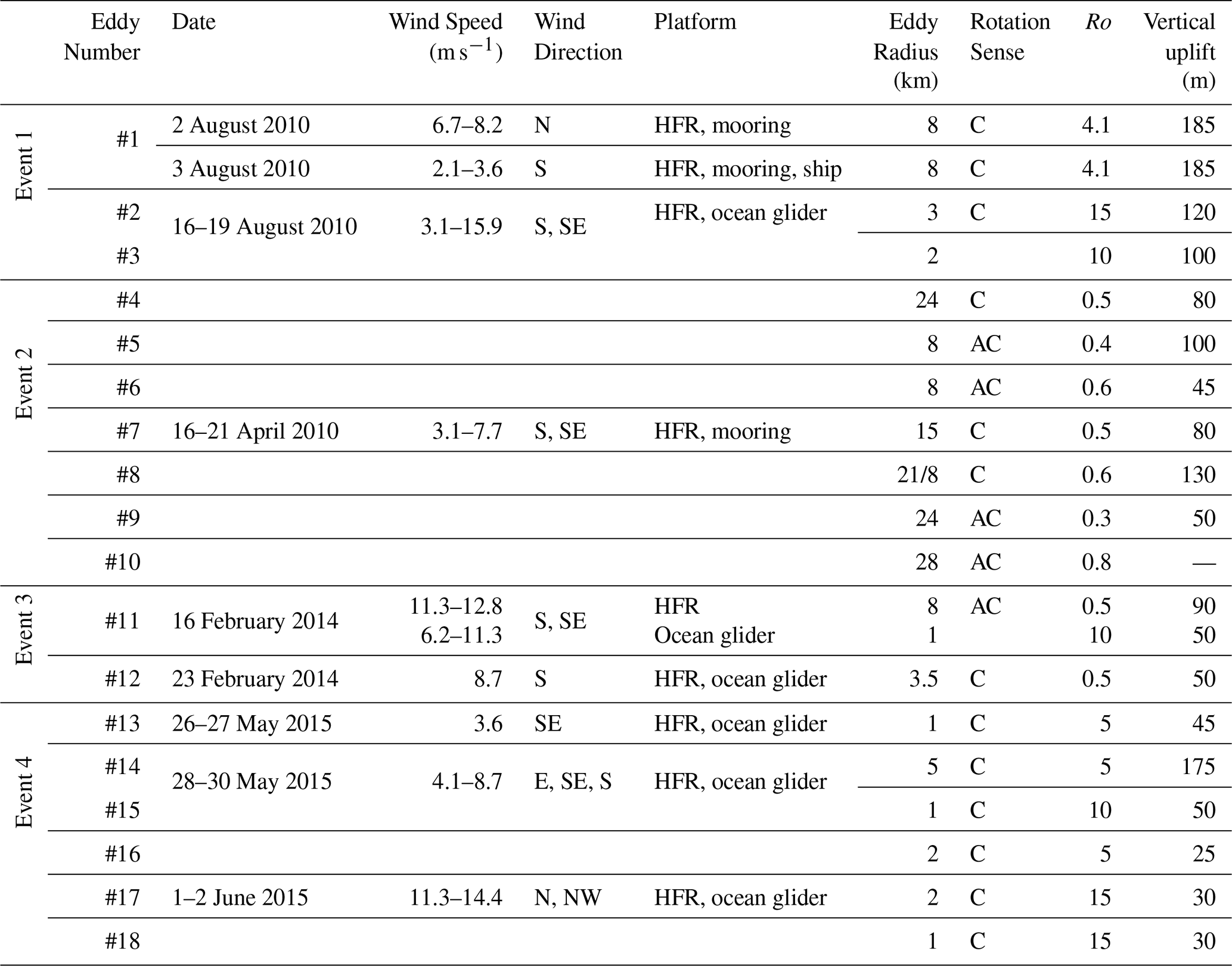
In this section, we present field measurements of 4 separate event periods detected using the different platforms in austral summer, autumn and winter (Table 2). The events included 18 different eddies with diameters 1–28 km with maximum Rossby number > 5 and a range of wind speeds.

3.1 Event 1 (shipborne/ocean glider): Mesoscale eddy and its peddies (August 2010)

Low SCC (0.3–0.4 mg m⁻³), warm core (∼ 21 °C) anti-cyclonic (counterclockwise) mesoscale eddy (> 20 km D) was present in the region over the period 2–4 August 2010 with centre at ∼ 114°59^′ E and ∼ 32° S (Fig. 2). Several cold core sub-mesoscale eddies and peddies can be clearly identified from the remotely sensed data either onshore or offshore in the south-west corner of the radar domain (Table 2).

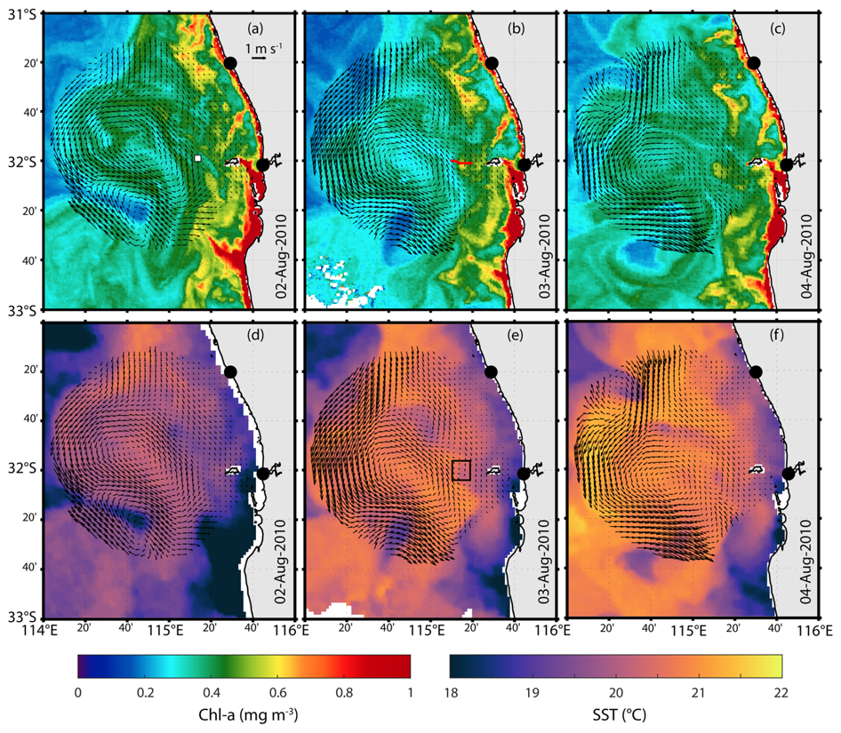
Figure 2 Remotely sensed (a–c) SSC, (d–f) Sea Surface Temperature and HFR surface currents (vectors) on 2–4 August 2010 (eddy #1, Event #1). The black dots represent HFR shore stations and the black-white square in (a) represents WACA20 mooring location (Fig. 1c). Red solid line in (b) is a ship transect on 3 August, and the black square in (e) represents the peddie location (eddy #1).

A cold core peddie (eddy #1, 8 km radius, Table 2; Fig. 2 b, c, e, f) appeared between 2–4 August 2010, to the west of Rottnest Island and migrated westwards before dissipating. A transect by R/V Southern Surveyor using the profiling towed body Nacelle crossed this feature on 03 August revealing a slanted cone (“distorted vertical cone”; Fig. 3b) shape in the vertical distribution of N-Chl that appeared to follow the local bathymetry. The N-Chl peaked at ∼ 0.7 mg m⁻³ below the surface with low concentrations below ∼ 75 m depth along the shelf and ∼ 150 m at deeper waters (Fig. 3b). Signatures of higher salinity, lower temperature, higher oxygenated water extending from ∼ 150 m depth towards the surface could be also seen from ship transect data (Fig. 3c–e). The vertical distribution of subsurface currents showed the signature of a cyclonic feature with westward (northward) flow offshore and eastward (southward) flow at the inner shelf. The peddie was also characterised by a relatively high Rossby number (|Ro$|\sim$ 4.1; Fig. 3f–h).

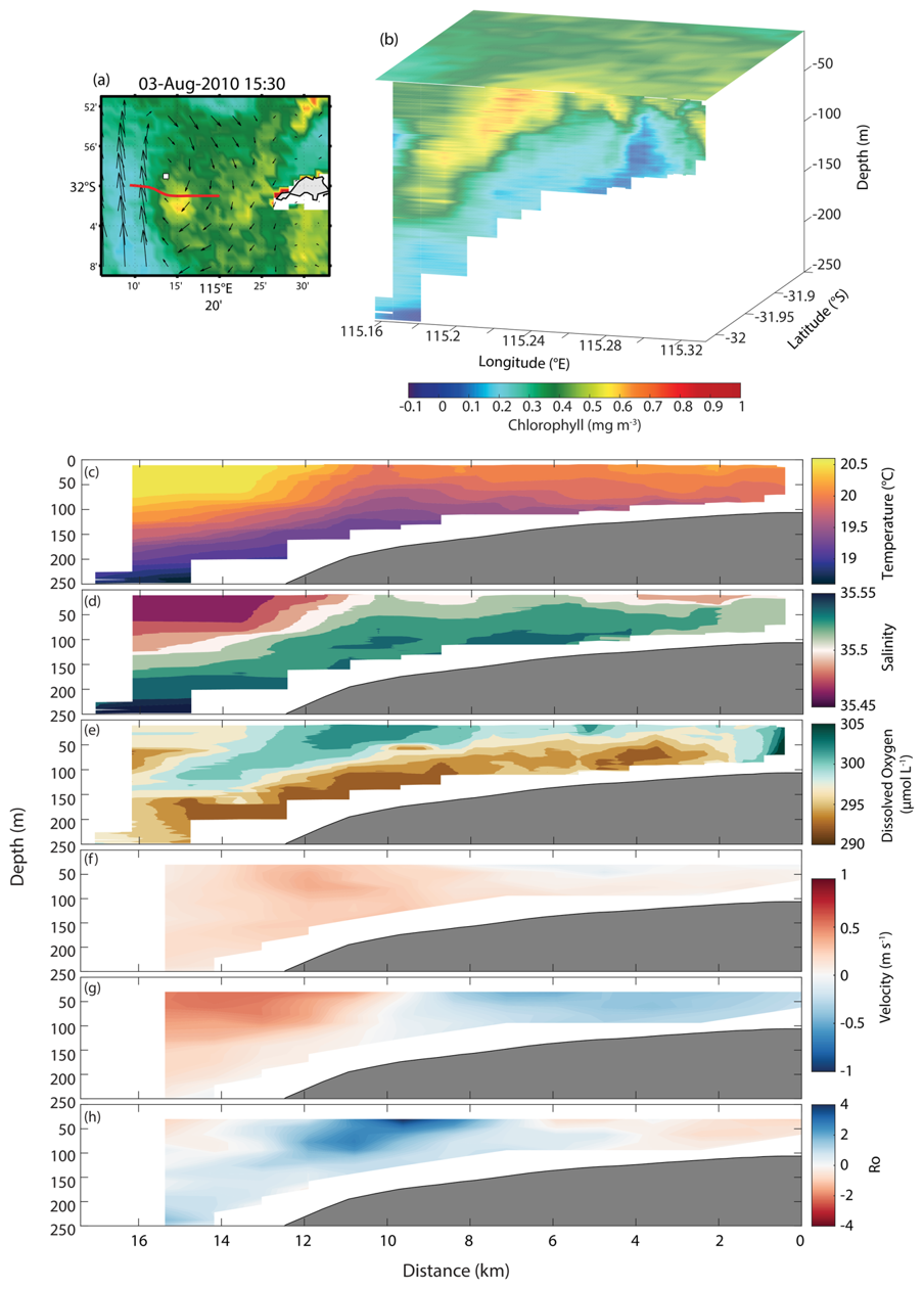
Figure 3 (a) SCC; (b) merged 3D structure of SCC (surface) and ship-based measurements N-Chl (subsurface), and (c–h) ship-based measurements of (c) temperature, (d) salinity, (e) dissolved oxygen, (f) u current component, (g) v current component, and (h) Rossby number on 3 August 2010 (eddy #1, Event #1). Red solid line in (a) is the ship-based transect shown in (b)–(h). Black-white square in (a) represents the WACA20 mooring location.

Similar features were observed in the mooring data (Fig. 4a, b): lower M-Chl (∼ 0.2 mg m⁻³) and slight increase in salinity (Figs. 2a, 4a), vertical uplift of colder water and cross-shore flow reversal (from east to west orientation) on 2 August 2010 (Fig. 4b–d). These features were consistent with upwelling at the centre of the peddie. Between 2–3 August, M-Chl concentrations reached 1 mg m⁻³ at the mooring location (Fig. 4a). The peddie on 3 August was characterised by colder water uplifting from 185 to 40 m depth, with a slight decrease in bottom M-Chl (< 0.5 mg m⁻³; Fig. 4a) and eastward (northward) flows (Fig. 4b–d). The slight decrease in bottom M-Chl values during 3 August was associated with increased M-Chl levels at the surface which was also consistent with peddie-induced upwelling (Figs. 2b, d; 3, 4).

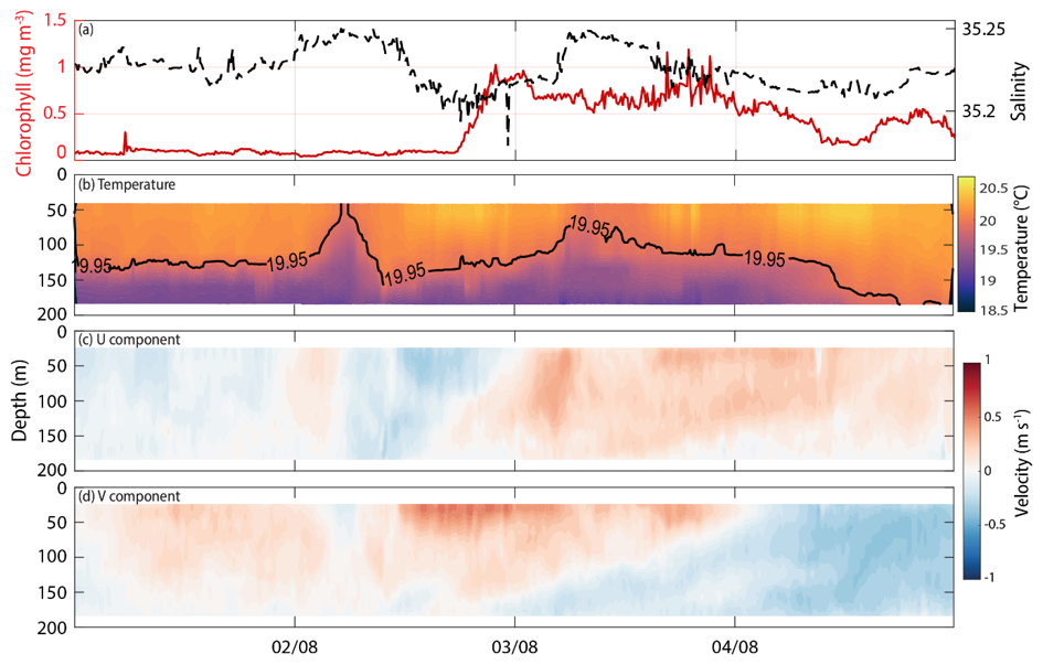
Figure 4 Mooring observations at WACA20 (Figs. 1c, 2a) in 1–4 August 2010 (eddy #1, Event #1) for (a) timeseries of M-Chl and salinity at 75 m depth, (b) temperature, (c) u component, and (d) v component.

Later in the same month (between 16–19 August), an ocean glider intersected and then was entrained into two rapid rotating (speed > 1 m s⁻¹; eddies #2 and #3; radius ∼ 2 km; Table 2) peddies. These peddies formed in the periphery of a sub-mesoscale eddy entraining colder and higher SCC closer to the coast (Fig. 5a, b). The peddies had a high Rossby number with |Ro$|>$ 10 and reached maximum DAC of 0.52 and 0.51 m s⁻¹ during the loops on 17 and 18 August, respectively (Fig. 5b). The uplift of colder (19.3 °C), higher salinity (34.45), low G-Chl and DO (0.4 mg m⁻³, 210 mM L⁻¹) water was detected in the cross-sectional vertical profiles (Fig. 5c, d, e).

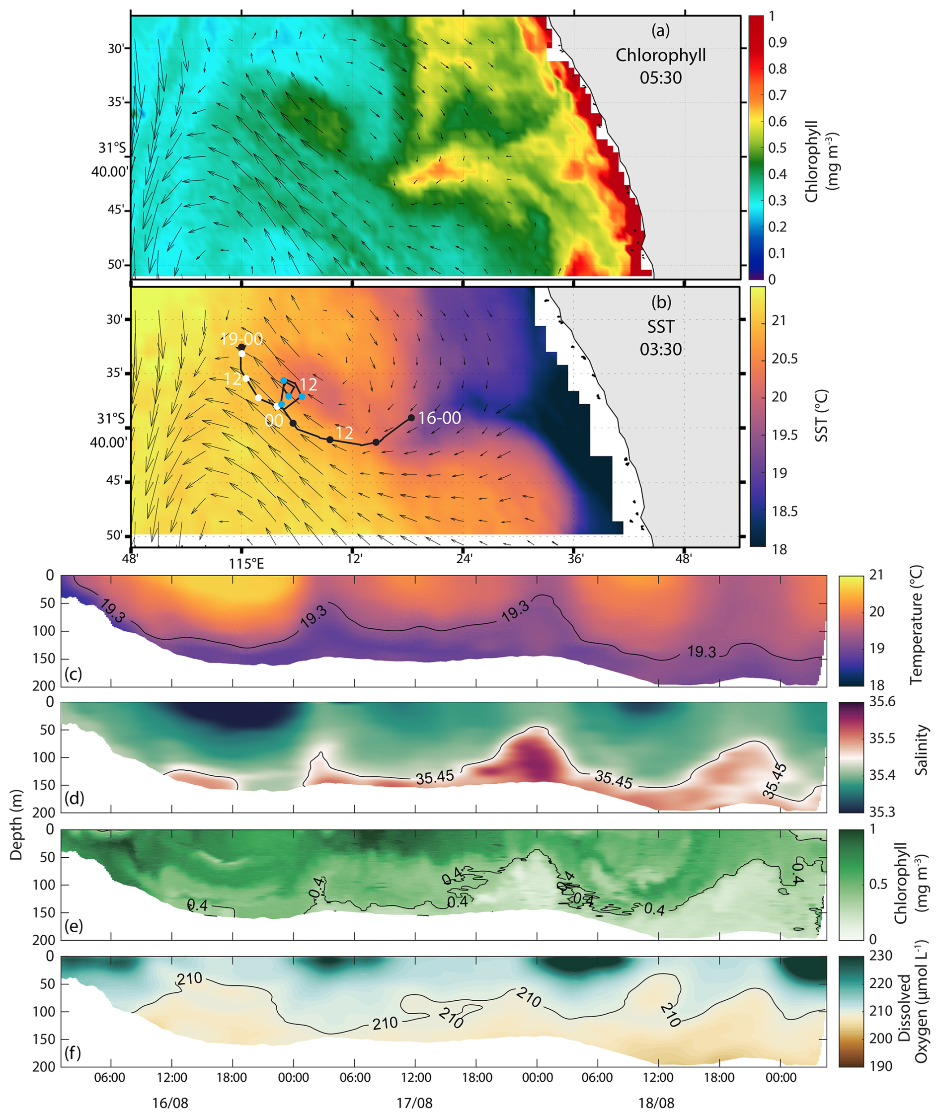
Figure 5 (a) SCC, (b) Sea Surface Temperature and HFR surface currents (vectors) on 16 August 2010. The black line represents glider track between 16–19 August 2010 (eddies #2–3, Event #1). The dots are at 6 h intervals and colour codes according to date: 16 (black), 17 (blue), 18 (white). Along-track glider distribution of (c) temperature, (d) salinity, (e) G-Chl, and (f) dissolved oxygen. E2 and E3 refer to eddy numbers show in Table 2.

3.2 Event 2 (ocean moorings): Sub-mesoscale eddy dynamics (April 2010)

Several cyclonic and anti-cyclonic eddies and peddies were observed within the HFR coverage and in proximity of the mooring sites between 16–21 April 2010 (Fig. 6). These features occurred under low to moderate (5–10 m s⁻¹) southerly and southeasterly wind conditions (Table 2) and all showed signatures of upwelling/downwelling.

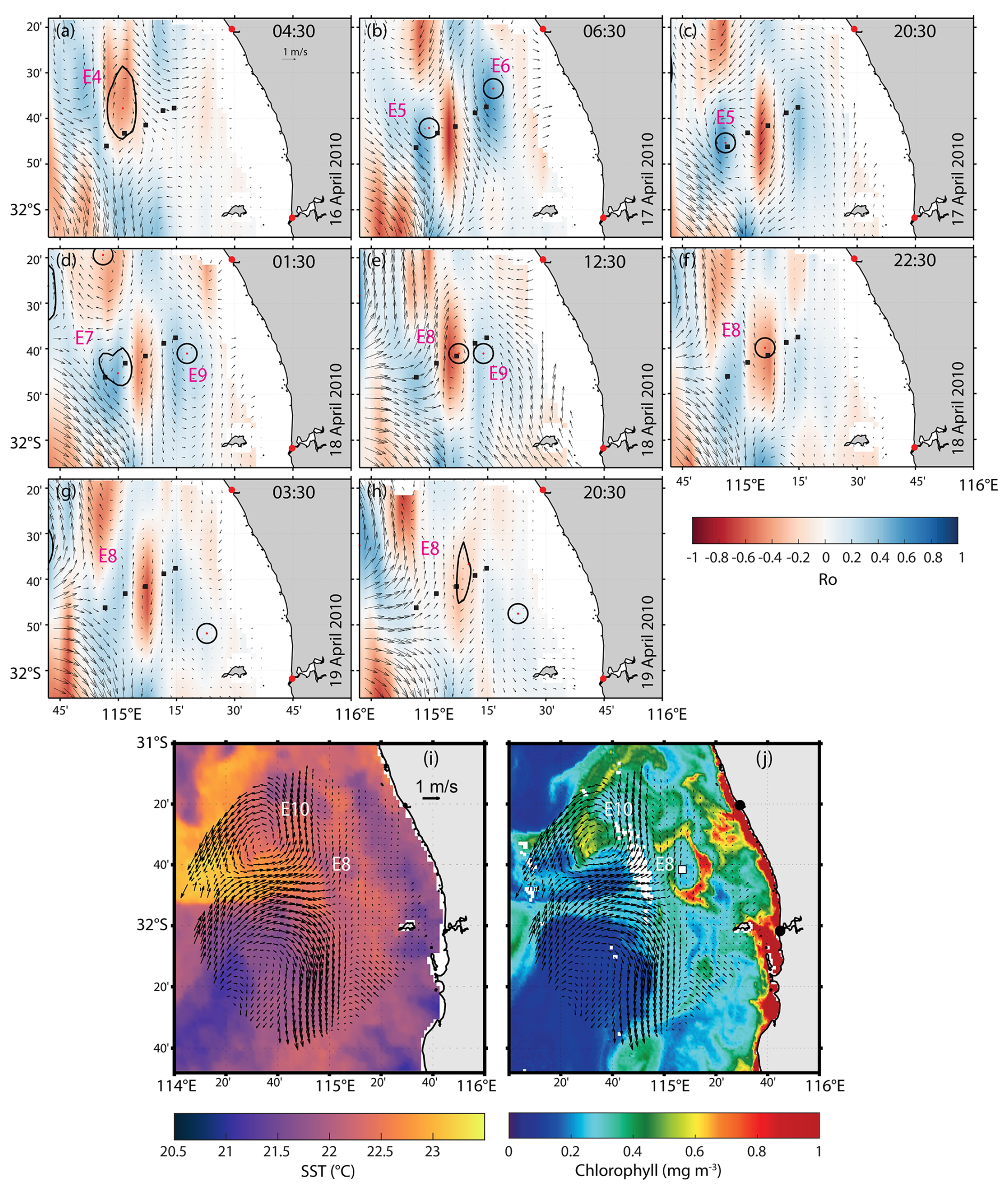
Figure 6 (a–h) HFR-derived Rossby number (in colour) and surface currents (vectors) occurring on 16–21 April 2010 (eddies #4–10, Event #2). (i) Sea Surface Temperature, (j) SCC, and HFR-derived surface currents (vectors) on 19 April 2010. In (a–h, j), mooring locations (Fig. 1c) are shown as black squares. Red dots and thicker black closed contour lines in (a)–(h) represent eddy centres and their shapes detected by the vector geometry algorithm. E4–E10 refer to eddy numbers shown in Table 2.

Isotherm displacements consistent with upwelling were observed in temperature profiles at WATR15 and WATR20 moorings when a sub-mesoscale cyclonic eddy (24 km radius; Table 2) was detected on HFR currents on 16 April. This eddy feature caused a vertical displacement of ∼ 80 m in the isotherms across moorings (eddy #4, Figs. 6a, 7d–f).

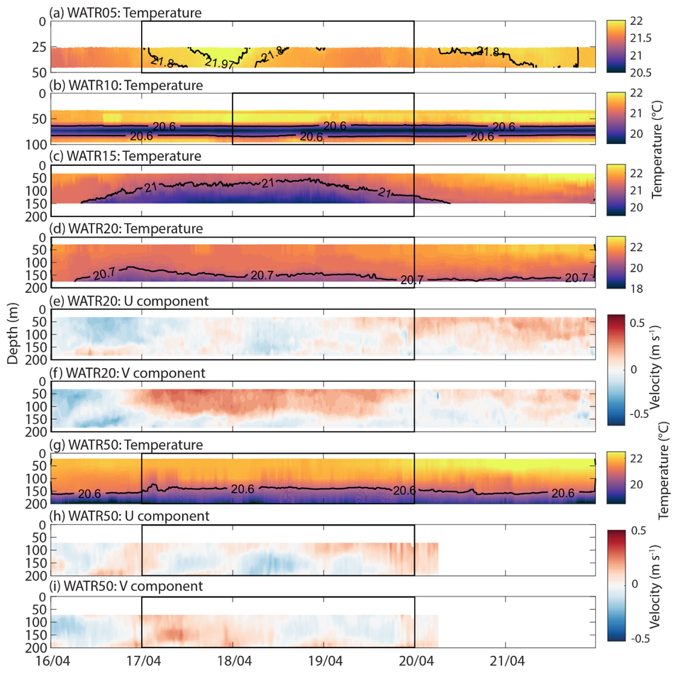
Figure 7 Mooring observations at (a) WATR05, (b) WATR10, (c) WATR15, (d–f) WATR20, and (g–i) WATR50 during 16 to 21 April 2010 (eddies #4–10, Event #2) for (a, b, c, d, g) temperature, (e, h) u component, and (f, i) v component. Black squares refer to eddy events shown in Fig. 6. Mooring locations are shown in Figs. 1c, 6.

A similar response was observed on 17 April when an anti-cyclonic peddie (8 km radius; Table 2) crossed WATR20 and WATR50 moorings, uplifting waters up to 100 m towards the surface (eddy #5, Fig. 7d–i). At the inner shelf, WATR05 mooring showed displacement of warmer water (∼ 21.97 °C) induced by an anti-cyclonic feature (eddy #6, Figs. 6b, c; 7a).

In the offshore region, an anti-cyclonic sub-mesoscale eddy (15 km radius; Table 2) approached the offshore mooring site (WATR50) on 18 April which vertically displaced isotherms by ∼ 80 m and reversed currents in the deeper layers (eddy #7, Figs. 6d; 7g–h). Along the inner shelf, a cold core cyclonic peddie (∼ 8 km radius) was observed near WATR15 which persisted until 19 April with variable dimensions (Table 2), transporting a patch of higher SCC at its periphery with a ∼ 130 m vertical displacement of the 21 °C isotherm (eddy #8, Figs. 6d–f, i, j; 7b, c). Inshore of the cyclonic peddie, an anti-cyclonic peddie also uplifted waters in the region (eddy #9, Figs. 6e; 7a, b). Offshore, a cold core anti-cyclonic eddy (eddy #10, 28 km radius) transported moderate-to-high SCC at its centre (Table 2; Fig. 6i, j).

3.3 Event 3 (ocean glider/mooring): Sub-mesoscale eddy and wind forcing (February 2014)

On 16 February 2014, an anti-cyclonic peddie (eddy #11, 8 km radius) was present along the inner shelf and close to the moorings (Table 2; Fig. 8a–c) under strong (> 10 m s⁻¹) southerly winds. Contrasting downwelling/upwelling signatures were identified at its centre and its periphery (Fig. 8d–f). An ocean glider tracked its southward movement and captured T, S, and G-Chl stratification with a subsurface DO maximum between ∼ 40–60 m depth (Fig. 8g–j). Whilst the peddie feature dissipated around midnight, measurements showed an upwelling feature in both temperature and salinity structures (0.4 km in radius; Table 2) aligned with strong currents and a high Rossby number (|Ro$|\sim$ 15; Fig. 8c, g, h).

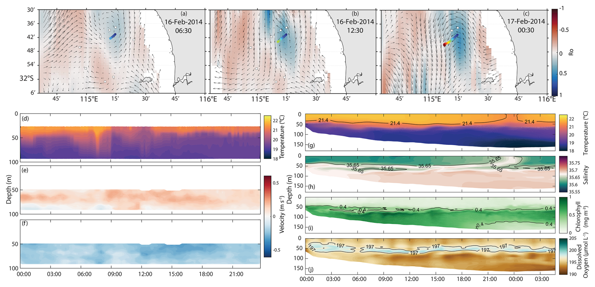
Figure 8 (a–c) HFR-derived Rossby number (in colour), surface currents (vectors), and glider tracking (in colour) on 16–17 February 2014 (eddy #11, Event #3). Mooring observations at WATR10 on 16 February 2014 for (d) temperature, (e) u component, and (f) v component. Cross-sectional ocean glider section on 16 February 2014 for (g) temperature, (h) salinity, (i) G-Chl, and (j) dissolved oxygen.

The dynamics at the periphery of an anti-cyclonic sub-mesoscale eddy and a small peddie under moderate (< 10 m s⁻¹) southerly winds were captured later in February when the glider moved from the inner shelf towards deeper water (eddy #12, Table 2; Fig. 9a). Along the periphery of the sub-mesoscale eddy in the inner shelf, colder and salty waters contrasted with warmer and lower-salinity waters offshore associated with the Leeuwin Current. Inside the peddie, isotherms (and isohalines) were uplifted to reach the surface within a few hours from its appearance. Despite the low velocities, the peddie (1 km radius; Table 2; Fig. 9) had |Ro$|\sim$ 3.

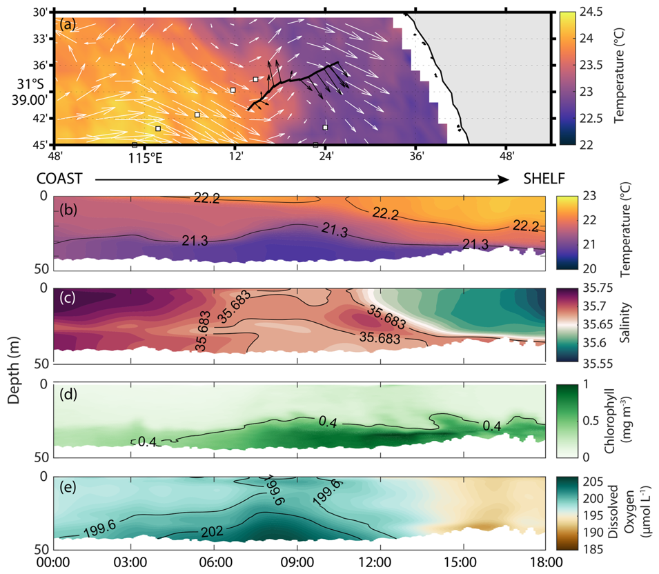
Figure 9 (a) Sea Surface Temperature and HFR surface currents (vectors) on 23 February 2014 (eddy #12, Event #3). Glider track and its depth-averaged velocities are shown in black in (a). Glider section along the tracking for (b) temperature, (c) salinity, (d) G-Chl, and (e) dissolved oxygen. Mooring locations are shown in (a) as black-white squares (see also Fig. 1c).

3.4 Event 4: Peddies Alley (ocean glider): fountains in the ocean (May–June 2015)

A glider deployment under different wind conditions was undertaken between 26 May and 2 June 2015. The winds were variable with (1) weak (∼ 3 m s⁻¹) southeasterly winds 26–27 May; (2) easterly and southerly winds 28–30 May; and (3) strong (> 10 m s⁻¹) northerly and north-westerly winds 1–2 June (Table 2). During 26–27 May 2015, the ocean glider travelled along the periphery of a cyclonic sub-mesoscale eddy and documented colder, saltier, denser waters to be uplifted within a peddie (eddy #13, 1 km radius; Table 2). The event occurred ∼ 21:00 UTC on 26 May (Fig. 10). Even under weak currents (< 0.3 m s⁻¹; Fig. 10h–i) and strong Rossby number (|Ro$|>$ 5), higher G-Chl and oxygenated waters prevailed close to the seabed (Fig. 10).

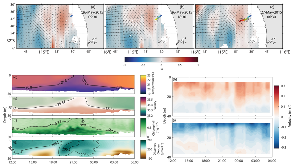
Figure 10 (a–c) HFR-derived Rossby number (in colour), surface currents (vectors), and glider tracking (in colour) on 26–27 May 2015 (eddy #13, Event #4). Cross-sectional ocean glider section on 26–27 May 2015 for (d) temperature, (e) salinity, (f) G-Chl, and (g) dissolved oxygen. Mooring locations are shown in (a)–(c) as black-white squares. Mooring observations at WATR04 (Fig. 1c) during 26–27 May 2015 for (h) u component, and (i) v component.

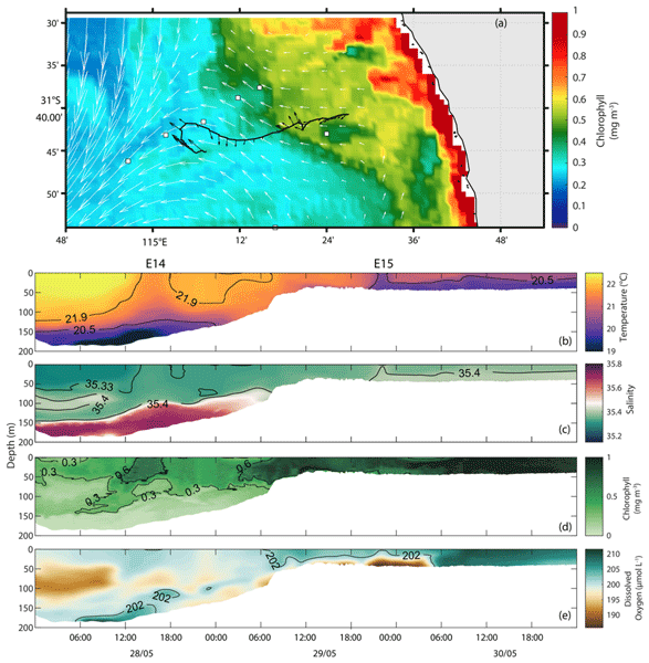
On 28–30 May 2015, the ocean glider mission continued tracking a region within high-G-Chl water entrainment (Fig. 11a). Closer to the shelf break, a peddie (eddy #14, 5 km radius; Table 2) displaced colder, more saline, denser waters with strong currents and Rossby number (|Ro$|\sim$ 8) restraining higher G-Chl and DO close to the surface (Peddie #1; Fig. 11). On the inner shelf, a patch of colder and dense water was trapped within a small peddie (eddy #15, 1 km radius; Table 2) in a region under higher G-Chl and lower DO (Peddie #2; Fig. 11a–d). Although the peddie's currents were weaker on the inner shelf, Rossby number |Ro$|>$ 5 was recorded.

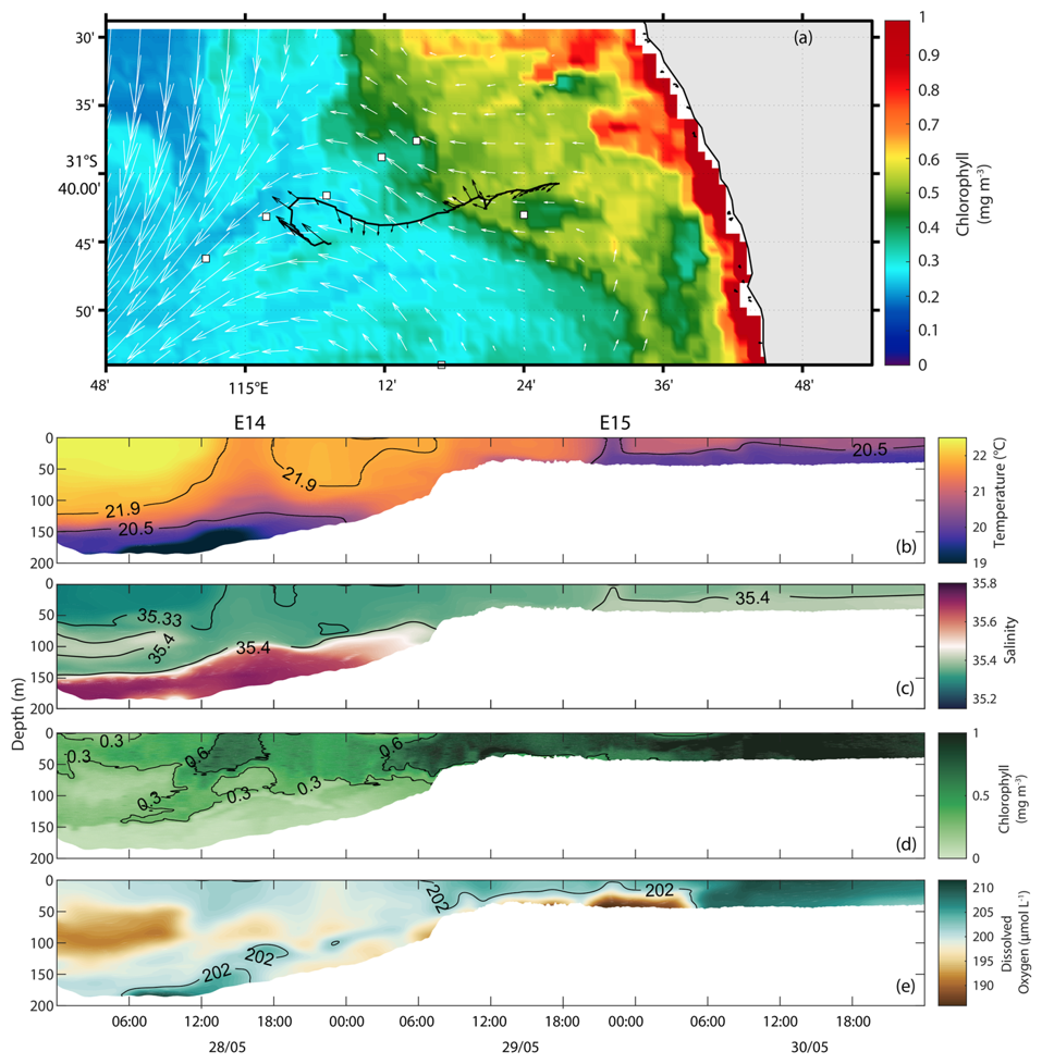
Figure 11 (a) SCC and HFR surface currents (vectors) on 30 May 2015 (Event #4). The black line represent glider track from 28 to 30 May 2015 (eddies #14–15, Event #4). Glider section along the tracking for (b) temperature, (c) salinity, (d) chlorophyll a fluorescence, and (e) dissolved oxygen. Mooring locations are shown in (a) as black-white squares (see also Fig. 1c). E14 and E15 refer to eddy numbers shown in Table 2.

Several peddies were identified close to the coast and towards the inner shelf during 1–2 June 2015 (Table 2; Fig. 12). Near the coast, colder (18–19.6 °C), denser, and saltier (35.44) waters were partially trapped in a peddie (eddy #16, 2 km radius) with weak currents (∼ 0.3 m s⁻¹) and high Rossby number (Ro > 10). This feature uplifted G-Chl (∼ 1 mg m⁻³) and highly oxygenated (> 208 µmol L⁻¹) waters towards the surface (Fig. 12). Another peddie (eddy #17, 2 km radius) with weak currents and a high Rossby number (|Ro$|\sim$ 10) was depicted around ∼ 15–18 h with warmer (20.1 °C) and slightly lower salinity (35.40) waters. This feature transported G-Chl (∼ 1 mg m⁻³) and low-to-moderate DO concentrations (∼ 203.5–206 µmol L⁻¹) towards the surface (Fig. 12). The last peddie (eddy #18, 1 km radius) was observed on 2 June around midnight with stronger currents (∼ 0.5 m s⁻¹) and Rossby number (|Ro$|>$ 10), warmer (20.3 °C) and lower-salinity (35.4) core with moderate G-Chl (∼ 0.5 mg m⁻³) and low DO (203 µmol L⁻¹) along the entire peddie structure (Fig. 12).

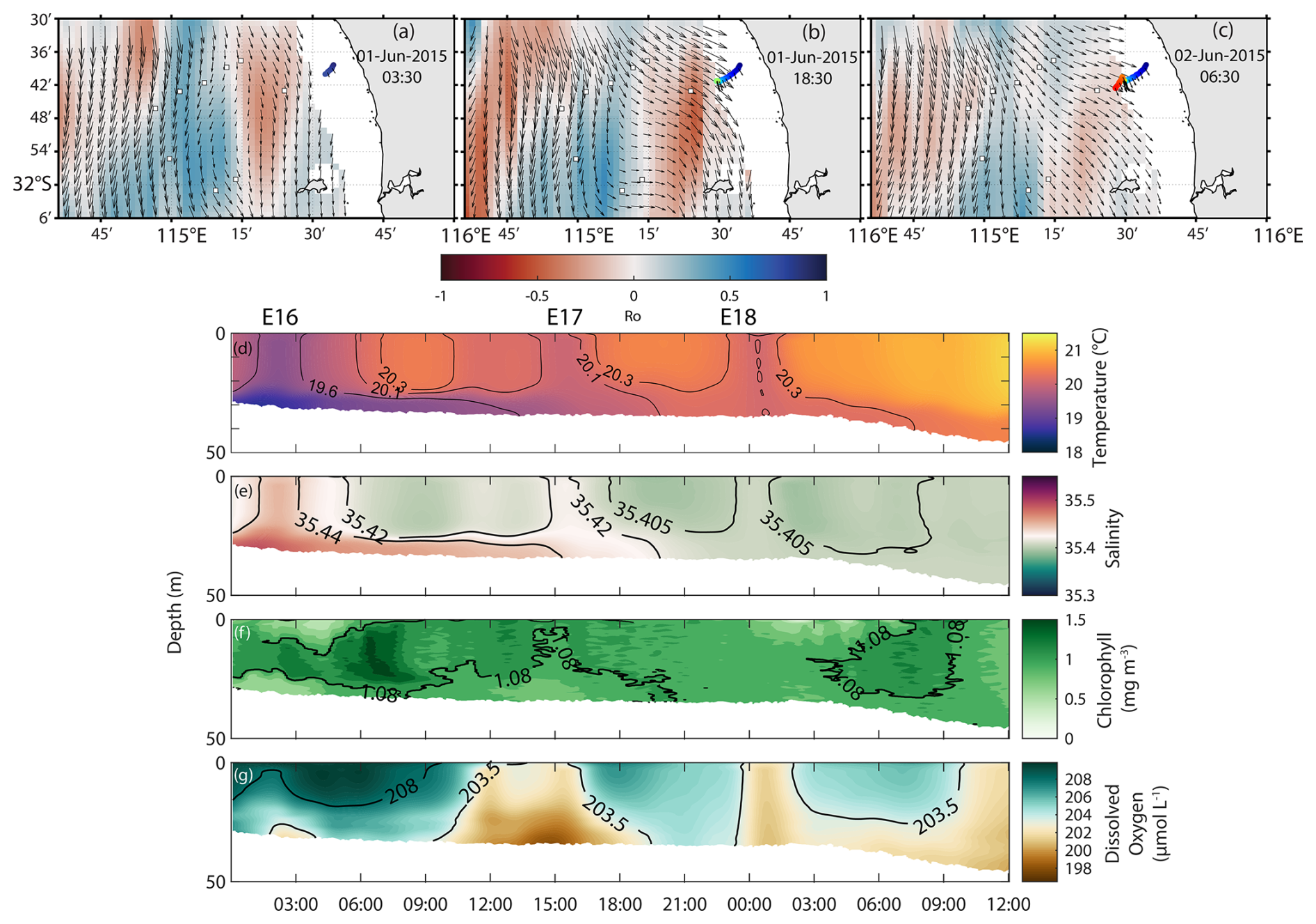
Figure 12 (a–c) HFR-derived Rossby number (in colour), surface currents (vectors), and glider tracking (in colour) on 1–2 June 2015 (eddies #16–18, Event #4). Cross-sectional ocean glider section on 1–2 June 2015 for (d) temperature, (e) salinity, (f) G-Chl, and (g) dissolved oxygen. Mooring locations are shown in (a)–(c) as black-white squares (see also Fig. 1c). E16–E18 refer to eddy numbers shown in Table 2.

4 Discussion

The simultaneous use of HFR, ocean gliders, moorings, satellite remote sensing, and shipborne measurements provides a rare multi-platform view of sub-mesoscale dynamics and their biogeochemical signature. By overcoming the spatial and temporal limitations of individual datasets, this approach offers insights into the three-dimensional physical and biogeochemical structure of sub-mesoscale eddies and their relationship with the forcing. It also allows us to link the observed eddies with the redistribution of dissolved oxygen and chlorophyll anomalies and to suggest a mechanism linking sub-mesoscale eddy upwelling to the uplift and redistribution of dense shelf water outflows. Overall, this multi-platform framework provides a comprehensive view of sub-mesoscale eddies, their circulation patterns and associated physical and biogeochemical structures, while providing direct evidence of their influence on biogeochemical variability in the Wadjemup Continental Shelf.

4.1 Sub-mesoscale eddy dynamics and their role in chlorophyll distribution

Along the Wadjemup Continental Shelf (WCS), sub-mesoscale eddies are short-lived (< 12 h) but ubiquitous features, particularly in regions with high horizontal shear along the interfaces of the Leeuwin Current and the periphery of mesoscale eddies (Figs. 2, 5; Bitencourt et al., 2025). Our observations, however, indicate that they can last for longer periods (up to 3 d) and may exert a more sustained influence on the shelf circulation and biogeochemistry (Figs. 2–4).

Most eddies exhibited high Rossby numbers (|Ro$|>$ 1, Table 2), indicative of ageostrophic dynamics, and intense vertical transport (Table 2), which modulated biogeochemical distribution along the shelf (e.g., Figs. 2–5). In particular, cyclonic eddies had |Ro$|>$ 1 and upwelled chlorophyll-rich, highly oxygenated waters from depths greater than 25 m (Table 2; Figs. 3–5, 10–12). These vertical velocities are consistent with previous theoretical and observational studies showing that sub-mesoscale eddies can generate intense vertical motions capable of transporting nutrients into the euphotic zone (e.g., Lévy et al., 2012; McWilliams, 2016). High Rossby numbers associated with submesoscale features indicate that processes other than geostrophic balance become important. In these conditions, centrifugal acceleration may play a significant role, potentially leading to gradient-wind or cyclostrophic balance, especially within compact and intense vortices (e.g., Pattiaratchi et al., 1987; McWilliams, 2016; Thomas et al., 2008).

Cyclonic sub-mesoscale eddies and peddies with |Ro$|>$ 5 were particularly associated with strong upwelling (up to 185 m, Table 2) and cyclostrophic balance (Figs. 5, 10–12), indicating intense vertical exchange within these structures. Anti-cyclonic eddies generally exhibited lower Rossby numbers (|Ro$|<$ 1) and were associated with downwelling of shallow waters (∼ 50 m; Table 2). However, anti-cyclonic eddies observed during event #2 (16–21 April 2010) were also associated with upwelling (Figs. 6c, d; 7b–d) and cyclostrophic balance despite their relatively low Rossby numbers (|Ro$|<$ 1; Table 2). This apparent discrepancy may reflect an underestimation of vorticity due to the relatively coarse spatial resolution of the HFR measurements, which would smooth velocity gradients and reduce the calculated Rossby numbers.

Sub-mesoscale eddies (and peddies) redistributed chlorophyll along the shelf through both horizontal advection and local accumulation (Figs. 2a–c, 5, 6i, j). Cyclonic eddies tended to accumulate chlorophyll along their periphery, whereas anti-cyclonic eddies retained it closer to their centres (Fig. 6i, j), consistent with observations in other coastal systems (Davila et al., 2021; Veatch et al., 2024). High DO concentrations within these eddies (e.g., Fig. 5) are consistent with enhanced photosynthetic production relative to local biological consumption. By rapidly injecting nutrients into the euphotic zone, these features may stimulate phytoplankton growth, trigger short-term blooms, and alter local primary production, with cascading effects on the structure and functioning of marine food webs (Figs. 2–5; Lévy et al., 2001, 2012). Mushroom-like structures were frequently associated with elongated chlorophyll filaments extending offshore (Fig. 1a), indicating strong lateral advection between adjacent eddies and enhanced transport of phytoplankton biomass. In oligotrophic regions such as the WCS, these processes can represent an important source of nutrients to coastal waters and create favourable feeding environments for larval species (Bitencourt et al., 2025).

4.2 Wind influence and dense water transport on sub-mesoscale eddies

Winds in the Wadjemup Continental Shelf control the circulation processes along the shelf in the absence of strong tidal forcing (Bitencourt et al., 2024; Mihanović et al., 2016). Previous work showed that southerly or southeasterly winds of ∼ 7–8 m s⁻¹ enhance pre-existing shear zones and promote the formation of sub-mesoscale eddies, whilst stronger winds (> 11–12 m s⁻¹) tend to disrupt or dissipate these structures (Bitencourt et al., 2025).

Under sea breezes and southerly winds on 23 February 2014, for example, eddy structures emerged to the surface (Table 2; Fig. 9). Diurnal sea-breeze cycle in WCS can efficiently generate near-inertial waves due to the local inertial period (∼ 24 h) that closely matches the diurnal wind forcing (Mihanović et al., 2016). These waves can propagate energy downward and enhance vertical shear well below the mixed layer (Mihanović et al., 2016), potentially contributing to the vertical mixing and thermohaline anomalies observed during periods of strong wind forcing (Fig. 9). Our observations during 16 February 2014 exhibit the influence of strong southerly winds (> 11 m s⁻¹) on evolution and stability (Fig. 8). As winds intensified, the eddy structure became increasingly elongated and eventually destabilized (Fig. 8a–c). This evolution coincided with colder and more saline waters reaching the surface (Fig. 8g, h), consistent with enhanced vertical mixing and upwelling. Strong winds may also contribute to eddy decay by extracting energy through wind stress curl (Teng et al., 2023) and by enhancing surface turbulence and vertical mixing (Zhang and Tian, 2014; Zhu et al., 2023).

In the WCS, Dense Water Shelf Transport (DWST) is a common occurrence due to strong air-sea heat fluxes associated with the Mediterranean climate, which generate dense waters that propagate offshore as gravity currents along the seabed (Mahjabin et al., 2019a; Pattiaratchi et al., 2011). Previous studies showed that dense shelf water transport/cascading off Western Australia is predominantly seasonal, occurring mainly during austral autumn and winter when evaporation-driven salinity increases and surface cooling enhance nearshore water density gradients (Mahjabin et al., 2019a, b). Our observations indicate that sub-mesoscale eddies (including peddies) can interact with these dense shelf water outflows (Figs. 5, 10–12). In particular, cyclonic sub-mesoscale eddies with |Ro$|>$ 1 entrained and uplifted portions of these dense shelf waters into the upper water column, with stronger DSWT uplift occurring under southerly winds and weaker uplift under northerly winds (Table 2; Figs. 5a, b; 10–12).

These observations suggest that sub-mesoscale eddies can play an active role in modulating the vertical transport and redistribution of dense shelf water outflows within the WCS (e.g., Fig. 5). In particular, these eddies may enhance vertical pumping of dense shelf waters and contribute to their redistribution within the upper water column (Table 2). Similar interactions between sub-mesoscale eddies and dense shelf water outflows have been reported in other coastal regions (Bosse et al., 2016; Fayman et al., 2019; Georgiou et al., 2020), highlighting the role of sub-mesoscale dynamics in modulating both horizontal and vertical transport along continental shelves.

4.3 Rossby number sensitivity and Force balance

Our multi-platform data set exhibited a wide range of Rossby numbers (Ro) across the selected events (Table 2). However, the different methods used to estimate Ro (Sect. 2.7) may introduce methodological uncertainties that affect direct comparisons between platforms. To ensure consistency, we recomputed Ro using a common formulation, Ro $=\frac{V}{fR}$, where V is the characteristic velocity, f is the Coriolis parameter and R the radius of curvature.

Using this formulation, Ro shows considerable differences between platforms (Fig. 13a) and previously calculated Ro (Table 2). For instance, the ship-based Ro during Event 1 indicates |Ro$|\sim$ 1, suggesting a flow regime where inertial and Coriolis forces are comparable. The HFR-derived Ro matching with ship-based observations (HFR-ship) on 3 August 2010 (Figs. 2, 3; Event 1, Table 2) shows a smaller value, indicating stronger rotational control and a greater influence of Coriolis forces. In contrast, ocean glider-derived Ro (Events 1, 3 and 4; Table 2) span a much wider range (|Ro$|\sim$ 1–20), with many observations exceeding 1. This indicates strongly ageostrophic conditions and suggests that centrifugal effects may become significant (Fig. 13a). HFR-derived Ro remain consistently small (|Ro$|<$ 0.5), implying that the flow appears predominantly geostrophic and/or that smaller features (≤ 10 km D) may be underestimated due to HFR relatively coarse spatial resolution.

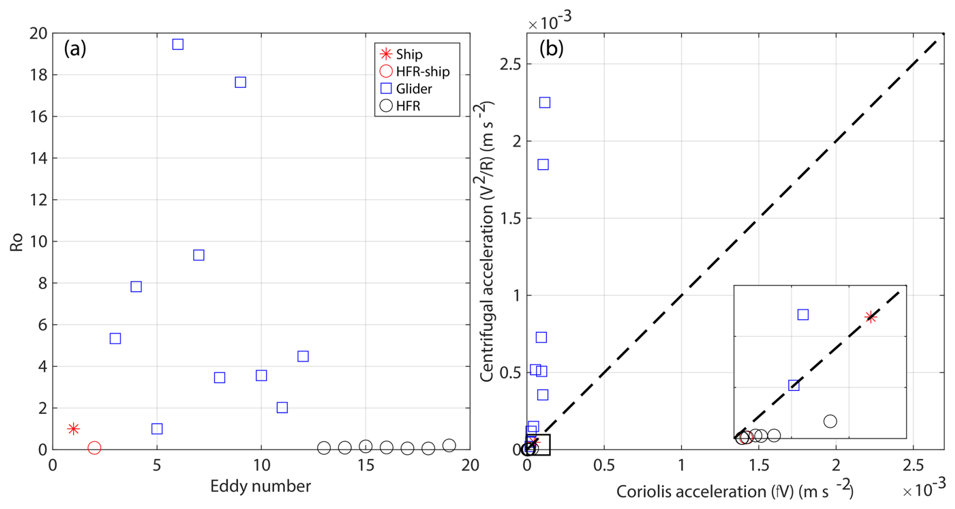
Figure 13 (a) Rossby number (Ro $=V/\left(fR\right)$) estimated for the selected events using different observing platforms: ship (red asterisk), HFR–ship (red circle) matching with ship transect (Event 1), glider (blue square), and HFR (black circle). (b) Centrifugal acceleration ($V^{\mathrm{2}}/R$) versus Coriolis acceleration (fV). The dashed line in (b) indicates the 1 : 1 relationship (cyclogeostrophic balance).

We also compared centrifugal and Coriolis accelerations to further evaluate their relative influence in these features. Most HFR observations cluster near zero, indicating weak centrifugal contributions relative to Coriolis acceleration and a predominantly geostrophic regime (Fig. 13b). The ship and HFR-ship estimates lie close to the 1 : 1 line (V²/R ≈ fV) (Fig. 13b), consistent with cyclogeostrophic balance, where centrifugal and Coriolis forces are of comparable magnitude (|Ro$|\sim$ 1). This suggests that HFR measurements mainly reflect larger-scale flows that remain closer to geostrophic balance.

Several ocean glider observations, in contrast, exhibited centrifugal accelerations comparable to or exceeding Coriolis acceleration (Fig. 13b), consistent with the large Rossby numbers inferred from ocean glider data (Table 2, Fig. 13a) and suggests a transition toward cyclostrophic balance, where centrifugal effects become dominant. Overall, this suggests that ocean glider measurements capture smaller-scale, more nonlinear structures where centrifugal effects become important.

5 Conclusions

This study investigated the physical and biogeochemical three-dimensional structure of sub-mesoscale eddies and peddies along the Wadjemup (Rottnest) Continental Shelf (Western Australia). A multi-platform data set was used, consisting of remote sensing, shipborne, mooring, and ocean glider measurements. Analyses outlined the role of a mesoscale eddies in the generation of sub-mesoscale eddies, their internal structures under different forcing conditions, and their potential contribution to chlorophyll distribution. The main conclusions can be summarised as follows:

• Sub-mesoscale eddies were found to occur primarily in areas of high shear, such as at the edges of Leeuwin Current, where the LC interacted with the wind-driven Capes Current, and at the periphery of larger mesoscale features in agreement with Bitencourt et al. (2025). Local winds contributed to the generation and dissipation of surface and near-surface eddies, also leading to the surfacing of underwater eddies.

• Localised upwelling and downwelling conditions commonly occurred within the eddies. Upwelling of isotherms (up to 185 m vertically) was recorded within cyclonic sub-mesoscale eddies. Anti-cyclonic eddies were found to promote both downwelling and upwelling.

• Mesoscale and sub-mesoscale eddies could lead to elevated chlorophyll levels in offshore regions and concentrations of high chlorophyll due to advection throughout the study area. In the presence of dense water outflows, sub-mesoscale eddies trapped, upwelled, and transported some of these waters offshore.