Furthest-first inversion for internal consistency adjustments in the biogeochemical data product GLODAPv3

The global ocean absorbs a significant portion of anthropogenic carbon dioxide (CO₂) emissions. Tracking the fate of absorbed CO₂ and its impacts requires an internally consistent global observational dataset spanning decades. In the Global Ocean Data Analysis Project (GLODAP), data from disparate research cruises are compared in a secondary quality-control process, adjusted for consistency where necessary and compiled into a data product. Differences between cruises are quantified with a crossover analysis, comparing data at depth (where natural variability is minimal) from nearby sampling stations, and an inversion algorithm calculates a set of adjustments that would minimise these differences globally. The adjustments are reviewed by an expert committee and a subset applied to produce the final data product. The previous major version (GLODAPv2) used a weighted least squares (WLSQ) approach for the inversion. However, several issues became apparent when applied to the GLODAPv3 dataset, primarily significant regional biases in calculated adjustments. To address these issues, a new inversion algorithm called furthest-first (FF) has been developed for use in GLODAPv3, which has been implemented in a freely available, open-source Python package (xover). Here, we describe the FF approach and test it on simulated datasets and by comparing it to WLSQ, finding that it produces accurate adjustments. We also show how the FF approach can be adapted (i) to avoid the regional biases that appear in WLSQ, (ii) to find an optimal set of adjustments accounting for the fact that some cruises will ultimately not be adjusted, and (iii) to approximately preserve selected trends in the cruise-by-cruise differences. Points (i) and (ii) above are addressed by a two-step variant of the approach denoted FF₂, which was applied in GLODAPv3. While FF represents a marked improvement on WLSQ for the GLODAP application, no algorithm can completely replace the role of expert judgement in the inversion process, for example when selecting convergence criteria, which cruises are permitted to be adjusted, and which trends should be preserved.

1 Introduction

The ocean has taken up almost 30 % of accumulated anthropogenic carbon dioxide (CO₂) emissions since 1850 (Friedlingstein et al., 2026), and approximately 90 % of the excess heat (Li et al., 2023). The consequences include ocean warming, acidification, and deoxygenation (Gruber, 2011). To quantify both the size of the changing ocean carbon sink and the consequences, internally consistent observations of marine carbonate system and other biogeochemical variables are needed. However, global ocean carbon and biogeochemistry data are produced by many laboratories using varied and evolving methods and equipment, meaning that systematic biases may exist, especially between older and newer datasets. This, exacerbated by the general sparsity of ocean observations, complicates the quantification and understanding of observed changes. As a response, the Global Ocean Data Analysis Project (GLODAP) was initiated in the late 1990s as an effort to synthesize a global bias-corrected dataset primarily for quantifying anthropogenic inorganic carbon in the ocean (Key et al., 2004). The goal of GLODAP is to create an internally consistent data product of carbon-relevant data for the world ocean, where all datasets are comparable through time and space such that long-term trends can be reliably determined. The emphasis is on internal consistency rather than absolute accuracy, because there is no established way to objectively determine the latter. That said, GLODAP aims not to change the regional or global averages of the variables it adjusts.

For the previous major version of GLODAP (GLODAPv2; Olsen et al., 2016) the “crossover and inversion” method was used for quality control (QC), as described by Tanhua et al. (2010), Gouretski and Jancke (2001) and Johnson et al. (2001). The crossover step compares deep (e.g., >1500 m) data from pairs of cruises that measured the same variable(s) within a defined distance of each other, and quantifies the differences (“offsets”) between them. In the inversion step, an adjustment is calculated for each cruise that would minimise its crossover differences. For both GLODAPv1.1 (Key et al., 2004) and GLODAPv2 (Olsen et al., 2016) the inversion was solved using a weighted least squares model (WLSQ) following Johnson et al. (2001), which was applied separately to different ocean regions. During the preparation of GLODAP version 3 (hereafter GLODAPv3), a global rather than regional inversion was attempted, which revealed several problems with the WLSQ approach.

The main symptom was strong spatial patterns in the calculated adjustments for certain variables. Damping the WLSQ model using a set of pre-defined core cruises (the weighted damped least squares, WDLSQ, solution) reduced the patterns but did not remove them entirely. The spatial patterns are not evident in the pre-inversion differences between cruises, have no apparent physical reason, and are not associated with different countries, laboratories or research groups. A network analysis revealed that the most likely cause is that while GLODAP cruises are well-connected by crossovers within the major ocean basins, they are relatively poorly connected by crossovers between cruises in different basins. This means that the apparent differences between basins probably reflect random uncertainties in cruise pair offsets in the connecting cruises, which do not average out to zero because of the scarcity of connections, rather than true regional biases that should be removed with adjustments.

It was challenging to understand the causes of this problem and rationalise the WLSQ adjustments because, from the user perspective, the method provides a solution in one step. Further, in versions prior to GLODAPv3, not all calculated adjustments were actually implemented. Instead there was an expert discussion and decision on each adjustment, and adjustments that were smaller than the minimum limits were ignored. As WLSQ actively eliminates apparent trends in pre-adjusted data, some calculated adjustments had to be ignored or manually modified in an attempt to preserve these trends. These decisions were all made to achieve the GLODAP goal of improved global consistency with as few adjustments as possible. However, making such expert decisions means that the results of the inversion may also no longer be appropriate, as each calculated adjustment is valid only in the context of the whole set of adjustments. If a particular adjustment is not made, then the whole set should be recalculated taking this into account. This means that while WLSQ is an appropriate solution to the problem, the way GLODAP has used this method in the past can be improved.

There are some additional technical issues with WLSQ. Because they optimise everything at once, least-squares models are sensitive to outliers. This means that one cruise with a big offset will skew the adjustment calculated for all cruises connected to it. In previous GLODAP versions, this problem was limited by applying pre-inversion adjustments to the strongest outliers and using weights to limit the influence of uncertain offsets, but these modifications do not remove the problem entirely. Additionally, the matrix used to specify crossover differences was highly overdetermined, and least squares models are generally acknowledged to be a poor choice for solving such matrices. The GLODAP matrices are also unevenly distributed, i.e., showing strong grouping, with many rows (crossovers) for a limited set of columns (cruises). Least squares methods are known to be sensitive to groupings such that the solution can easily be biased towards groups. Finally, the WLSQ model minimises the individual crossover differences, not the average difference for each cruise. This means that individual cruises are likely to end up with non-zero average offsets after adjustment.

Here, we present a new inversion approach, designed to circumvent the problems above, called furthest first (FF). FF is a type of coordinate-descent optimisation (Wright, 2015), where cruises are adjusted separately and iteratively starting with those with the greatest offsets. It includes the capacity to not adjust a selected subset of cruises, while still accounting for their offsets, and to preserve selected temporal trends in the offsets. We describe the FF method, which has been implemented in an open-source Python package (xover; Humphreys, 2025). Simulated crossover networks have been used to validate the FF calculations, and the results for real GLODAPv3 datasets have been compared with WLSQ calculations, including quantitative and qualitative overviews of the differences between the methods. FF has been used for the inversion analysis for GLODAPv3, and the companion data description paper contains more details for that specific application (Lange et al., 2026).

2 Methods

2.1 Crossover analysis

The crossover analysis is an objective way to detect systematic differences between two cruises with measurement profiles in close spatial proximity (Gouretski and Jancke, 2001). To minimise the effect of natural (e.g., seasonal) variability on differences between cruises, data are compared only in the deep part of the water column (typically > 1500 m, though this has varied; Olsen et al., 2016) where such variability is small, and between stations within a lateral distance threshold, which has varied from 100 to 300 km in different versions of GLODAP, but this variation has not significantly affected the results of the crossover analysis.

In general terms, a “cruise” is a subset of data that was measured and calibrated together such that any systematic bias in the values should be consistent and can be eliminated using a constant correction across the whole subset. Usually this corresponds to an individual oceanographic expedition identified by a common expedition code (expocode). However, in some circumstances an alternative approach might be needed, for example to account for differences between legs of an expedition or offsets between different instruments used to measure the same variable.

GLODAP uses the “running cluster” variation of crossover analysis (Tanhua et al., 2010), in which each individual profile from cruise i is compared to all profiles from cruise j that fall within the distance threshold by interpolating to a series of depth, potential temperature or density levels. This is repeated for all profiles in cruise i, and then a weighted mean offset and weighted standard deviation are calculated across the levels. The weighting is such that levels with less scatter have a larger influence on the mean. If cruise i has at least three profiles that overlap with cruise j, then a final crossover difference (c_i,j) is calculated, and these differences are compiled into a crossover matrix. The crossover difference for c_j,i is assumed to be equal to $-c_{i,j}$, rather than being evaluated separately.

For some variables, it may be more appropriate to calculate crossover differences as multiplicative rather than additive differences (Lauvset and Tanhua, 2015). These must be converted into percentage differences (e.g., 1 % rather than 1.01) when inserting into the crossover matrix, because the algorithm attempts to minimise all values in this matrix.

A weight can be assigned to each crossover to modulate its influence on the calculated adjustments. How these weights should be assigned may vary by the application. For GLODAPv3, the calculated weights are mainly based on the inverse of the standard deviation of the offsets calculated from each profile in cruise i that overlaps with cruise j. The weights are then further scaled by a series of factors that influence our confidence in each crossover, representing the differences in time between cruises, lateral temperature and density gradients, depth and number of crossover data points, and statistical quality. For a detailed explanation, see the GLODAPv3 data description paper (Lange et al., 2026).

2.2 Furthest-first inversion

2.2.1 Overview of the furthest-first approach

Furthest-first (FF) inversion is a form of coordinate-descent optimisation. Briefly, the FF inversion procedure works as follows. Cruise weighted mean offsets (c_i,s for cruise i, where s refers to the iteration step; Appendix A) are calculated for all cruises, and the cruise with the largest c_i,s normalised to its uncertainty is adjusted to exactly eliminate its offset. In other words, the cruise that lies furthest from its neighbours is adjusted first. All c_i,s values are then recalculated accounting for the adjustment, and these steps are repeated until some convergence criterion is reached. During the procedure, some cruises may be adjusted multiple times, with each successive adjustment refining the overall adjustment value after adjacent cruises have also been adjusted, while others may never receive any adjustments. Some cruises can be fixed to receive pre-defined (e.g., zero) adjustments, and temporal trends in variables can be selectively and approximately preserved. The following sections describe the procedure in more detail.

2.2.2 Initial setup

For each variable that will receive adjustments, an n × n crossover matrix C_ij of offsets between pairs of cruises (Sect. 2.1) is assembled, where n is the total number of cruises in the dataset. Each element of C_ij contains the offset between cruises i and j such that its value is positive if the data from cruise i are greater than those from cruise j and negative otherwise. The matrix is therefore skew-symmetric (i.e., ${\mathbf{C}}_{ij}=-{\mathbf{C}}_{ji}$). The main diagonal and any elements where no offsets could be calculated (Sect. 2.1) are set to zero. The weights assigned to the c_i,s are also assembled into an n × n symmetric matrix W_ij, again with zeroes on the main diagonal and where no offsets are available.

An n × n adjustment matrix A_ij,0 is initialised, containing all zeros. The values in A_ij,s are updated on each iteration (s) of the FF routine.

An n × n date-difference matrix D_ij of the time interval between each pair of cruises is calculated. Each element of D_ij contains the date of cruise i minus the date of cruise j, in decimal years. D_ij is therefore skew-symmetric, like C_ij.

A length n vector r_i of trends (rate of change) in the crossovers is computed. Each element of r_i contains the slope of a weighted least squares regression of the corresponding rows of C_ij against D_ij, weighted by W_ij. A threshold should be applied to determine whether a trend can be computed for each cruise, for example based on the number of crossovers, with trends that are not computed assigned as zero. Any calculated trends judged to be spurious (how best to judge this may vary by application) and thus not retained in the inversion can also be assigned as zero in r_i.

A trend-adjusted crossover matrix T_ij is calculated:

$$\begin{array}{}\text{(1)}& {\displaystyle }{\mathbf{T}}_{ij}^{\prime }={\mathbf{C}}_{ij}-{\mathit{r}}_i{\mathbf{D}}_{ij}\text{(2)}& {\displaystyle }{\mathbf{T}}_{ij}=({\mathbf{T}}_{ij}^{\prime }-{\mathbf{T}}_{ij}^{\prime \mathrm{T}})/\mathrm{2}\end{array}$$

where superscript T denotes the transpose of the matrix. ${\mathbf{T}}_{ij}^{\prime }$ is similar to C_ij, but it is no longer skew-symmetric. Each element of ${\mathbf{T}}_{ij}^{\prime }$ contains the crossover difference between cruises i and j, corrected for the trend in cruise i. As each of cruises i and j has a different set of crossovers, their trends are rarely identical. This asymmetry can lead the adjustments calculated by the iterative solver to drift considerably rather than converge. The second step of the calculation, Eq. (2), resolves this by averaging the values for each pair of cruises. Each element of T_ij is thus corrected for the average of the trends in cruises i and j, and T_ij is skew-symmetric. If it is not desired for the inversion to attempt to preserve any apparent trends, then C_ij can be used instead of T_ij in all subsequent calculations, and D_ij and r_i do not need to be computed.

For calculating the uncertainties associated with the weighted mean offsets calculated in the next section, the effective sample size (k_i) is computed from the weights matrix (Kish, 1965):

$$\begin{array}{}\text{(3)}& {\mathit{k}}_i={\displaystyle \frac{({\sum }_j{\mathbf{W}}_{ij}{)}^{\mathrm{2}}}{{\sum }_j{\mathbf{W}}_{ij}^{\mathrm{2}}}}\end{array}$$

The critical t-distribution value for each element of k_i, denoted t_i, is also computed. This contains values for the inverse of the cumulative distribution function of the Student's t distribution with the degrees of freedom specified by k_i and at a desired confidence level (here, 1σ). When multiplied by the standard error of c_i,s in the next section (Eq. 7), t_i gives the 1σ confidence interval for the mean offsets.

Finally, a length n Boolean vector p_i may be assembled to identify a set of cruises that are not permitted to be adjusted in the inversion. Cruises that are permitted to be adjusted are assigned as true in p_i and those that are not, false. Cruises that are not permitted to be adjusted are still accounted for in the rest of the inversion procedure (e.g., when calculating weighted mean offsets). This can be used during a complete inversion if certain cruises will not be adjusted. In GLODAPv3, it will also be used for the annual minor version releases, where adjustments are calculated for and applied to newly added cruises, but the adjustments for existing cruises in the product are not revisited.

2.2.3 Iteration procedure

The matrices T_ij, W_ij and A_ij,s (where s denotes the iteration step, starting with s=0) are used to calculate the vector of weighted mean offsets for each cruise, c_i,s:

$$\begin{array}{}\text{(4)}& {\mathit{c}}_{i,s}={\displaystyle \frac{{\sum }_j({\mathbf{T}}_{ij}+{\mathbf{A}}_{ij,s}){\mathbf{W}}_{ij}}{{\sum }_j{\mathbf{W}}_{ij}}}\end{array}$$

Determining the uncertainty in each weighted mean offset (u_i,s) then requires several further calculations. First, the residuals between the individual crossovers and the cruise weighted mean offsets are calculated (R_ij,s):

$$\begin{array}{}\text{(5)}& {\mathbf{R}}_{ij,s}={\mathbf{T}}_{ij}+{\mathbf{A}}_{ij,s}-{\mathit{c}}_{i,s}\end{array}$$

The weighted variances (${\mathit{\sigma }}_{i,s}^{\mathrm{2}}$) are then computed as

$$\begin{array}{}\text{(6)}& {\mathit{\sigma }}_{i,s}^{\mathrm{2}}={\displaystyle \frac{{\mathit{k}}_i{\sum }_j{\mathbf{W}}_{ij}({\mathbf{R}}_{ij,s}{)}^{\mathrm{2}}}{({\mathit{k}}_i-\mathrm{1}){\sum }_j{\mathbf{W}}_{ij}}}\end{array}$$

and are converted into 1σ confidence intervals for each offset (u_i,s):

$$\begin{array}{}\text{(7)}& {\mathit{u}}_{i,s}={\mathit{\sigma }}_{i,s}{\mathit{t}}_i/\sqrt{{\mathit{k}}_i}\end{array}$$

Cruises that have crossovers with only one other cruise are assigned a default uncertainty value, which could be adapted depending on the analysis. For GLODAPv3, we used double the standard deviation of all c_i,s at the corresponding iteration step.

Only the cruise with the largest absolute normalised offset is adjusted during each iteration, as follows. An adjustment vector (a_i,s) is created as a copy of c_i,s; all elements in a_i,s representing cruises that are not permitted to be adjusted (based on p_i) are set to zero; and then all remaining elements other than the one with the maximum absolute value after normalising to uncertainty are also set to zero:

$$\begin{array}{}\text{(8)}& {\mathit{a}}_{i,s}=\left\{\begin{array}{ll}{\mathit{c}}_{i,s}& \text{where }\left(\text{abs}\right({\mathit{c}}_{i,s}/{\mathit{u}}_{i,s})=\text{max}(\text{abs}({\mathit{c}}_{i,s}/{\mathit{u}}_{i,s})\left)\right)\text{ and }{\mathit{p}}_i\\ \mathrm{0}& \text{otherwise}\end{array}\right.\end{array}$$

The adjustment matrix is updated by adding the adjustment vector to its columns and subtracting it from its rows:

$$\begin{array}{}\text{(9)}& {\mathbf{A}}_{ij,s+\mathrm{1}}={\mathbf{A}}_{ij,s}+{\mathit{a}}_{i,s}-{\mathit{a}}_{j,s}\end{array}$$

Equations (4) to (9) are repeated until some convergence criterion is reached (Sect. 2.2.4).

After the final round of adjustment, the 1σ confidence intervals are calculated with Eq. (7) and these can be reported as the cruise-level uncertainties in the final adjusted values. These values can be compared with the pre-inversion adjustment confidence intervals to assess how much the cruise-level uncertainties have been reduced by the adjustment process.

2.2.4 Convergence criteria

The FF routine can be stopped after a set number of iterations or when some threshold is reached, for example based on the size of the adjustments being calculated (which virtually always decreases from one iteration to the next) or some statistic related to the c_i,s values (i.e., cruise weighted mean offsets). Care must be taken if using adjustment size as a convergence criterion, because, while the adjustments added in subsequent iterations might be individually negligible, they can add up to a significant total change (Sect. 3.1.2).

Two different approaches were developed and tested using simulations and the real GLODAPv3 dataset. First, we ran the inversion with all cruises permitted to be adjusted (i.e., p_i=True for all i), for enough iterations (at least 1 million) for all calculated adjustments to reach steady state with respect to continued iterations. This first approach is referred to as FF₁.

Second, we used a two-step approach. The aim here was to apply an approximate minimum threshold to the size of the adjustments that would be calculated. To begin, the FF inversion was run with all cruises permitted to be adjusted but with a cut-off for stopping iterations at 5 % of the threshold. For example, for dissolved inorganic carbon (DIC) and total alkalinity, the target adjustment threshold was 2 µmol kg⁻¹, so the iterations were stopped once suggested absolute adjustments became smaller than 0.1 µmol kg⁻¹. After this point, p_i was updated such that any cruise with an absolute adjustment after this set of iterations of less than the total threshold would never be permitted to be adjusted. In the examples given here, the total threshold was kept at 2 µmol kg⁻¹, but its value could be revised at this point for example to account for regional variations (Lange et al., 2026). The inversion was then restarted from the beginning with the updated p_i and run until steady state. This second, two-step approach was used for the final GLODAPv3 analysis and is referred to as FF₂.

2.2.5 Software implementation

The FF inversion approach has been implemented in a free and open-source Python package called xover (Humphreys, 2025, https://github.com/mvdh7/xover, last access: 20 October 2026). This is built upon several other Python packages including JAX (Bradbury et al., 2018), NumPy (van der Walt et al., 2011; Harris et al., 2020), SciPy (Virtanen et al., 2020) and Statsmodels (Seabold and Perktold, 2010).

2.3 Simulated crossover networks

In order to test the FF inversion, we designed an approach to generate arbitrary networks of crossovers with similar statistical properties to the GLODAPv3 network, specifically that for DIC. In a simulated network, the true offsets between cruises and any trends are exactly known, because they are assigned.

A series of crossover networks were simulated with different settings (e.g., size of the random offsets; magnitude and type of the trends), including some with and without additional random noise, to investigate how well the FF inversion could retrieve the assigned offsets and trends under different conditions. For each configuration, multiple different networks were simulated with different random number generator seeds to check that our interpretations of the results were generally applicable, rather than being specific to one particular network.

3 Results and discussion

3.1 FF validation with simulated networks

3.1.1 Reproducing assigned offsets and trends

For simulated networks without noise (i.e., where each crossover exactly represents the assigned offset between its pair of cruises), FF₁ inversion successfully converges on adjustments that are perfectly correlated with the assigned offsets, with a slope of 1. FF₂ inversion converges on adjustments with a good correlation with the assigned offsets close to the ideal slope of 1, with some scatter that scales with the size of the target adjustment threshold (Sect. 2.2.4). In both cases, there can be a small constant bias, because the inversion is designed to target internal consistency between cruises and does not explicitly attempt to minimise the average size of adjustments: adding a constant value to the data for all cruises does not affect the differences between them. The bias is not significant relative to the uncertainties in the overall inversion process, especially when using real datasets, and it could be removed by subtracting the average adjustment from all adjustments after inversion. Either way, a small global bias would not be inconsistent with GLODAP's mission to produce a dataset that is internally consistent while making no claims about its absolute accuracy. However, it should be accounted for as a source of uncertainty for the most accurate work, as it would affect the apparent internal consistency of marine carbonate system calculations.

Random noise was also added to the simulated crossover offsets to represent the fact that the data from one particular profile of a cruise may not exactly reflect the overall bias of the cruise. Both FF₁ and FF₂ still worked reliably, calculating adjustments that were well correlated with the assigned offsets and with the scatter about the correlation scaling with the spread of the added random noise.

The GLODAPv3 analysis uses data from deeper than 1500 m, on the assumption that there should generally be no significant natural variability through time in biogeochemical variables there. However, in some regions this may not be accurate (e.g., Perez et al., 2018), and where clear trends are observed in pre-inversion offsets, the manual QC process has previously tried to avoid eliminating these trends with adjustments. Our simulations confirm that without trend preservation (i.e., using C_ij instead of T_ij; Sect. 2.2.3), FF₁ does eliminate virtually all temporal trends in cruise offsets. On the other hand, using T_ij leads to a good correlation between trends before and after inversion (r²=0.75; RMSD = 0.06 µmol kg⁻¹ a⁻¹; Fig. 1a). The results for trend-preserving FF₂ are very similar to FF₁, with an r² of 0.97 between the two approaches (Fig. 1b).

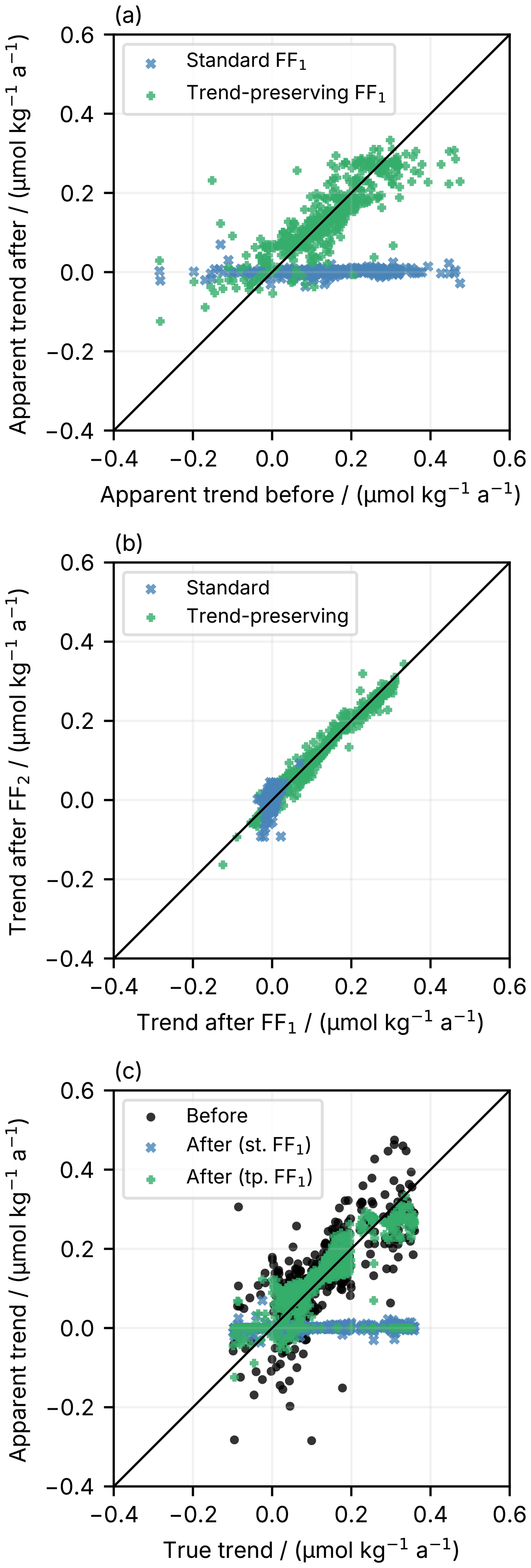
Figure 1 Relationships between assigned and apparent temporal trends before and after FF inversion for a simulated cruise network including random noise in crossover values. Each data point represents a single cruise in the network, black diagonal lines show the ideal 1 : 1 relationship. (a) Trends compared before and after FF₁ inversion with (trend-preserving) and without (standard) trend preservation with T_ij. (b) Comparison between trends computed after FF₁ and FF₂ inversion. (c) Apparent trends computed from the crossover matrix before and after the standard (st.) and trend-preserving (tp.) FF₁ inversion compared with the true trends assigned in the simulation.

The correlation between trends before and after inversion is not perfect, but simulation results where the true trends are known shows that this is expected. First, the trends determined from the pre-inversion crossover matrix C_ij do not perfectly represent the true assigned trends (r²=0.46; RMSD = 0.093 µmol kg⁻¹ a⁻¹; “before” in Fig. 1c). The pre-inversion trends are calculated from uncorrected data so the biases in the cruises that the inversion seeks to solve will also cause incorrect trends to be targeted. There is thus uncertainty in the target trend for FF to preserve. Also, trends are averaged across two cruises in Eq. (2), so the “target” trend will already not be exactly the same as either cruise's own trend. This means that cruises connected to other cruises with compatible trends will generally have their trends preserved, but not otherwise, which is desirable, because a trend not supported by connected cruises is more likely to be spurious.

Real-world datasets have additional complications. Each cruise spans a different geographic extent and trends might therefore differ across the cruise. The crossovers it has are with different cruises at different spatial points where the trend might be different than the average for the first cruise. Real-world trends also normally display variability and changes over time.

Despite these limitations, our simulations show that the trends after trend-preserving FF more closely resemble the true assigned trends than before inversion. In the example shown in Fig. 1c, the root-mean-square difference (RMSD) between the apparent trends and the true assigned values is ∼ 20 % lower after trend-preserving inversion than before inversion.

3.1.2 Convergence of the FF solution

In simulated networks, convergence within well-connected “clusters” of cruises – representing regions or ocean basins within the real dataset – happens relatively quickly (e.g., within ∼ 5000 FF iterations for a GLODAP-like network of ∼ 500 cruises), and then these clusters are drawn together over a much greater number of iterations (Fig. 2). The rate at which clusters converge depends on how well-connected they are, with the real GLODAP dataset taking towards 1 000 000 iterations to converge if all cruises are permitted to be adjusted (Fig. 2). Essentially, cruises within the better-connected clusters are adjusted so that they are internally consistent within the clusters first, and then these clusters as a whole converge towards the cluster containing the greatest number of cruises. This cluster convergence takes many more iterations, as multiple cruises have to be shifted together.

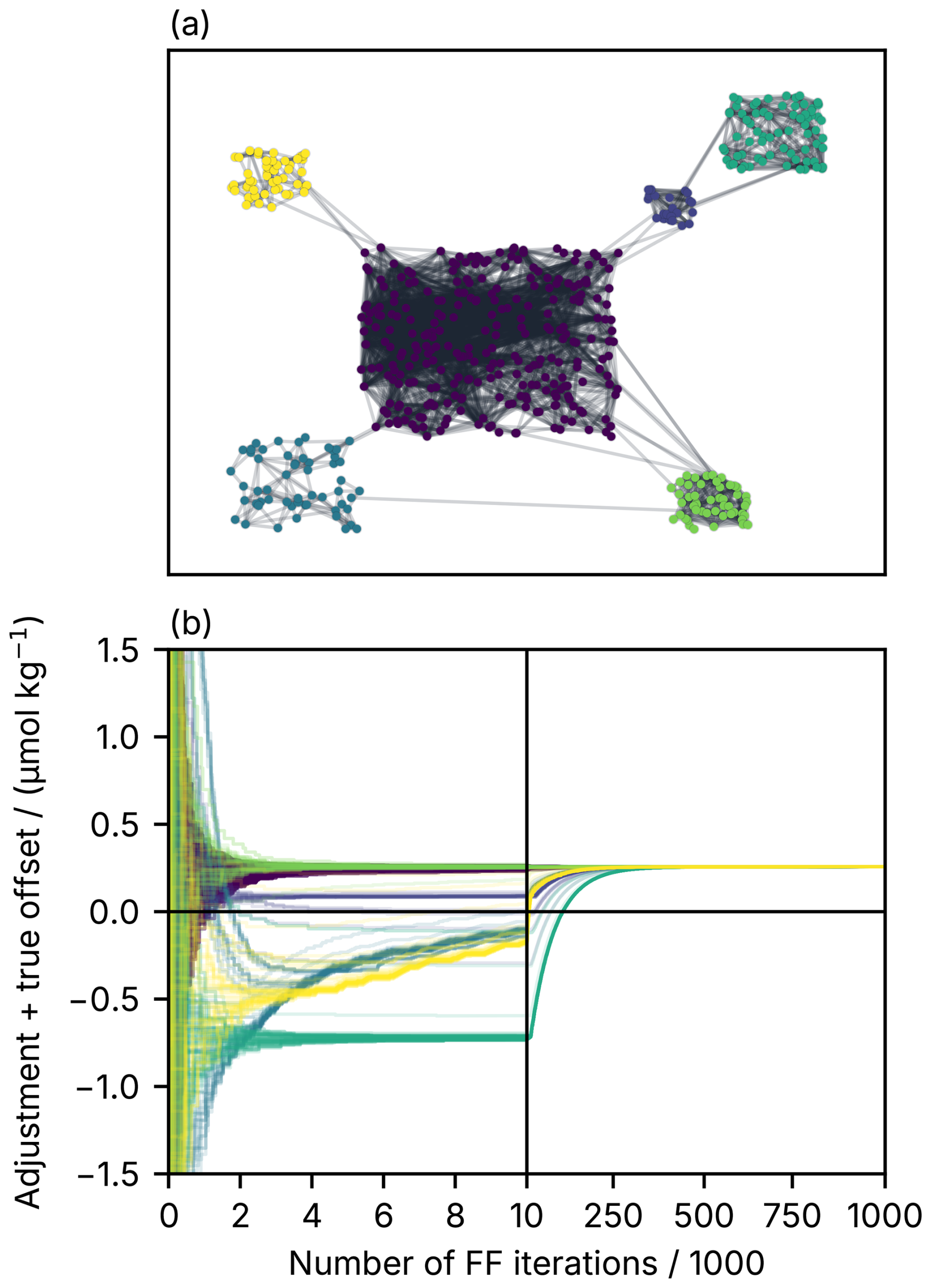
Figure 2 (a) Network graph for the simulation used to illustrate convergence of clusters in (b). Each coloured circle represents a cruise, and the lines show crossovers between cruises. The colours mark the different clusters; these do not correspond to real ocean basins. (b) Cruise adjustments normalised to their true assigned offsets through the inversion process for a simulated dataset. Each line represents a different cruise and the colours match (a), showing the “regions” in the dataset. The final adjustments + offsets converge on a globally biased value of around 0.25 µmol kg⁻¹, close to where the largest cluster (dark blue) initially converges, as discussed in Sect. 3.1.2. Note the change in horizontal axis scale at 10 000 iterations, indicated by the vertical black line.

It is necessary for the crossover matrix to be symmetrical for the solution to converge reliably. Trends can be slightly more accurately preserved by not symmetrising the trend-corrected crossover matrix, i.e., using ${\mathbf{T}}_{ij}^{\prime }$ instead of T_ij in the inversion. However, using ${\mathbf{T}}_{ij}^{\prime }$ generally causes the FF iterations to fail to converge, because for each pair of cruises i and j, the adjustment that should be applied to minimise the offset from the perspective of i is generally inconsistent with that from the perspective of j. This means that there is a continuous drift in adjustments upon continuing iterations, so no usable solution is returned.

3.1.3 Uncertainties in adjusted cruises

We find overall reductions in the cruise-level uncertainties (u_i,s; Eq. 7) after FF inversion both in simulations and tests with real data. Using the GLODAPv3 DIC dataset as an example, FF₂ inversion with a minimum adjustment cut-off (Sect. 2.2.4) adjusts 24 % of ∼ 500 cruises and reduces the average cruise-level uncertainty to ∼ 80 % of its pre-inversion value. This reduction in uncertainty is consistent across all cruises, including those that were not permitted to be adjusted. Using FF₁ inversion with all cruises adjusted reduces this uncertainty further to 50 % of pre-inversion. These numbers support the statement that the FF₂ approach used by GLODAP attempts to maximise internal consistency of the data product while still avoiding small or uncertain adjustments.

3.2 Comparison between FF and WLSQ inversion

3.2.1 Quantitative results

As discussed in Sect. 1, for the GLODAPv3 dataset, the WLSQ inversion returned adjustments for some variables with significant regional biases, where roughly consistent adjustments were calculated across entire regions. While the WLSQ result was mathematically valid, adjusting an entire region is not consistent with the GLODAP philosophy, which prefers to make as few adjustments as possible, and it conflicts with our earlier reasoning (Sect. 1) that the apparent regional differences are more likely an artefact of random uncertainties in the limited number of cruises that connect between regions than a true bias. We will use the real GLODAPv3 DIC dataset as an example in this section.

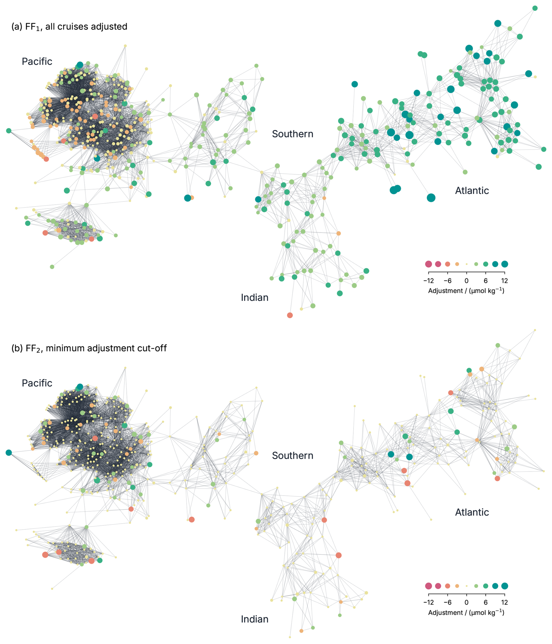
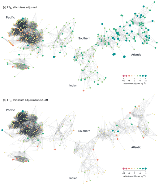
Figure 3 Network graph for the real GLODAPv3 DIC dataset. Each node (circle) represents a cruise and the edges (lines) represent crossovers used in the inversion. The colours and sizes of the nodes indicate the adjustment value calculated by the inversion. (a) FF₁ inversion with all cruises adjusted. The WLSQ inversion results produce a virtually identical pattern except with all values ∼ 2.4 µmol kg⁻¹ lower (Sect. 3.2.1). (b) FF₂ inversion with a minimum cut-off for adjustments applied, as used for GLODAPv3.

For the same dataset, the FF₁ inversion returns a similar set of regional biases (Fig. 3a) with an almost perfect correlation with the WLSQ adjustments (r²=0.999; Fig. 4a). This demonstrates that FF does converge on a valid set of adjustments. The mean adjustment for the WLSQ approach is virtually zero, while FF₁ gives a mean adjustment of ∼ 2.4 µmol kg⁻¹. This discrepancy is not unexpected given that the approach does not have an explicit constraint to hold some particular average value constant, as discussed in Sect. 3.1.1. Again, it would be perfectly valid to add or subtract a constant from all calculated adjustments to have an average of zero.

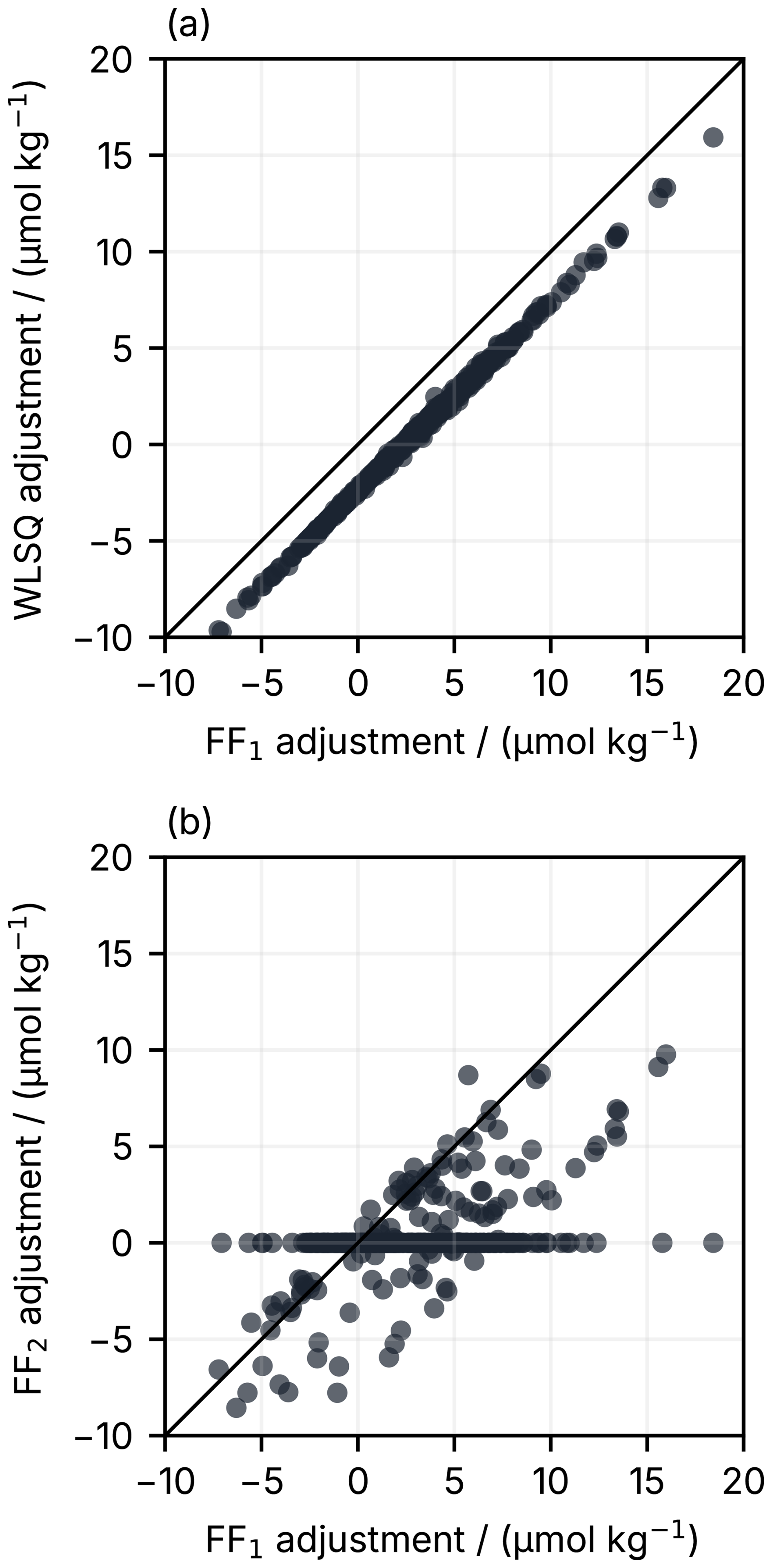
Figure 4 Comparisons between adjustments calculated by the different inversion approaches for the real GLODAPv3 DIC dataset. Diagonal black lines show the ideal 1 : 1 relationship. (a) FF₁ compared with WLSQ, where all cruises are permitted to be adjusted in both cases. (b) FF₁ with adjustments permitted for all cruises compared with FF₂ with a minimum cut-off for adjustments.

When implemented globally, the two inversion approaches (WLSQ and FF₁) both indicate that there appears to be a bias of around 6 µmol kg⁻¹ between the Atlantic and Pacific regions. WLSQ corrects the bias by adjusting the Pacific downwards and the Atlantic upwards, whereas FF leaves the Pacific roughly at zero and adjusts the Atlantic upwards more. Which of these (or any other) options is correct is a subjective judgement that cannot be determined objectively by any inversion method. Figure 3 shows that the Pacific contains more cruises than the other regions and that these are all very densely connected. FF₁ therefore adjusts the other cruises towards this more densely packed region, as discussed further in Sect. 3.2.2. This conceptual explanation is provided for context, and we reiterate that GLODAP has never used a global WLSQ nor FF₁.

However, if a cut-off is used to adjust only a subset of the cruises (i.e., FF₂), then a different pattern emerges: the regional biases disappear, and the pattern of adjustments is more random (Fig. 3b), as we expect. The adjustments are correlated with the FF₁ version, but there are significant differences (Fig. 4b). This highlights that choosing not to adjust some cruises changes the adjustments that should be used for other cruises, and it is not valid to select only a subset of points to adjust from WLSQ or FF₁. The adjustment calculated for a given cruise depends on if and how the cruises around it are also adjusted. Using FF₂ eliminates this problem with the GLODAP strategy that only became apparent after a global WLSQ was attempted.

In some applications, the FF₁ solution may be more appropriate to apply than FF₂. Determining which option to use requires expert analysis of the results and understanding of the underlying system. In this instance, as discussed in more detail in the GLODAPv3 data description paper (Lange et al., 2026), we can see that the different ocean basins are relatively poorly connected together; for example, the Pacific and Indian-Atlantic are connected by a single cruise in the Southern Ocean (Fig. 3). This means that entire regions are shifted to satisfy apparent offsets in a very small number of connecting cruises. If these offsets are thought to be meaningful then FF₁ might be appropriate. On the other hand, if they are more dominated by random noise in the individual offsets then using FF₂ is better.

3.2.2 Qualitative differences

The main motivation for investigating alternative approaches to the WLSQ method used in earlier versions of GLODAP was that the WLSQ results had unusual features that were difficult to interpret such as the apparent regional biases when applied globally. From the user perspective, the calculation proceeds in a single step that returns the full set of calculated adjustments in one go, which means that it is challenging to rationalise why a particular unexpected adjustment has been made and thus to decide whether or not to accept it. The FF approach is simpler to understand, and the solution can be investigated one iteration at a time to see why a particular adjustment has been calculated. The regional patterns in the DIC adjustment discussed in the previous section are a clear example.

The practical difference between WLSQ and FF can be thought of as analogous to the difference between a mean and a median. Consider a cluster of connected cruises where one “bad” cruise has a large true offset but all others are “good” with near-zero offsets. The WLSQ solution treats the cluster together and will calculate a smaller than necessary adjustment for the bad cruise, compensated for by also requiring a small constant adjustment to all of the good cruises. On the other hand, the FF would adjust the bad cruise first, bringing it into line with the good cruises, for which no constant adjustment would be required. However, in the real world we do not necessarily know which cruises are good and which are bad. FF assumes that if a large number of cruises agree with each other and a smaller number disagree, then the majority are correct, which may not always be the case. For example, if lots of cruises were conducted by one particular laboratory and that laboratory does have biased results, then a single cruise passing through the same area with data from an unbiased laboratory would receive an erroneous adjustment. If such a case were identified through independent evidence, both WLSQ and FF could be initialised with a correction to the biased dataset(s), eliminating the problem.

In earlier versions of GLODAP, some cruises had such large offsets that they skewed the results of the WLSQ inversion. This problem was circumvented by iteratively applying manual pre-inversion adjustments to these cruises before running WLSQ. With FF, such pre-inversion adjustments are generally not necessary, because isolated cruises with very large offsets will be adjusted first so the adjustments for the cruises connected to them will not be adversely affected by their initial presence. However, if there is some independent reason (i.e., not as a result of the crossover analysis) why a specific correction is thought to be appropriate for a cruise, then it is still advisable to apply this before running FF. The FF approach also has the capability of preserving temporal trends in the crossovers to some extent, as discussed in the previous section. WLSQ behaves more like the standard FF, actively eliminating any trends. It might be possible to devise an equivalent adaptation for WLSQ, but to the best of our knowledge, this has not yet been done.

4 Conclusions

The FF inversion method can calculate a set of adjustments that are consistent with the WLSQ solution, but with additional flexibility to adjust a subset of cruises and approximately preserve selected temporal trends. The FF₂ variant, where a two-step process is used to identify a subset of cruises with smaller offsets to not adjust, effectively eliminates the problem of regional biases that appear under WLSQ and FF₁, which is desirable for the GLODAPv3 application. It also ensures that the final set of adjustments are optimal accounting for the fact that not all cruises will be adjusted. The conceptual simplicity of the FF approach allows the reasons for particular adjustments to be investigated in greater detail. However, while inversion algorithms are an invaluable starting point for the QC process, decisions must still be made such as choosing convergence criteria, which cruises to permit the algorithm to adjust, and which trends it should attempt to preserve. Therefore, no algorithm can completely replace expert assessment.

Appendix A: Glossary of symbols

All matrices are shape n × n and all vectors length n.

Symbol	Description
i	A matrix row
j	A matrix column
n	Total number of cruises
s	An iteration step
ai,s	Adjustments per cruise (Eq. 8)
ci,s	Cruise weighted mean offsets (Eq. 4)
ki	Effective degrees of freedom (Eq. 3)
pi	Cruises permitted to be adjusted (Sect. 2.2.2)
ti	Critical t distribution values (Sect. 2.2.2)
ui,s	Standard errors in cruise weighted mean offsets (Eq. 7)
σi,s	Weighted standard deviations of residuals (Eq. 6)
Aij,s	Adjustment matrix (Sect. 2.2.2; Eq. 9)
Cij	Crossover matrix of offsets between cruises (Sect. 2.2.2)

Dij	Date-difference matrix of time intervals between cruises (Sect. 2.2.2)
Rij,s	Matrix of crossover residuals (Eq. 5)
${\mathbf{T}}_{ij}^{\prime }$	Trend-adjusted crossover matrix (Eq. 1)
Tij	Symmetrised trend-adjusted crossover matrix (Eq. 2)
Wij	Crossover weights matrix (Sect. 2.2.2)