Energetic near-inertial waves induced by winter storms and mesoscale eddies in the subtropical Northwestern Pacific Ocean

Near-inertial waves (NIWs) play a fundamental role in transferring wind energy into the ocean interior and sustaining diapycnal mixing, yet their wintertime characteristics and interactions with mesoscale eddies remain insufficiently understood. Using subsurface mooring observations and reanalysis products in the subtropical Northwestern Pacific Ocean, we investigate the generation, downward propagation, and modal characteristics of NIWs associated with two winter storm events. Although the wind energy input into the mixed layer during the first storm is approximately three times larger than that during the second storm, the observed near-inertial kinetic energy (NIKE) in the thermocline is comparable between the two events. Energy transfer analyses show that mesoscale eddies extract about 46 % of the wind-generated near-inertial energy during the first event, whereas they supply approximately 43 % of the wind input to NIWs during the second event. Although the opposing transfers may contribute to the comparable NIKE observed during the two events, given the observational limitations, the terms of near-inertial energy radiation out of the observed region and energy dissipation cannot be quantified directly but may also contribute to the observed NIKE. Additionally, the two NIW events exhibit distinct vertical wavelengths, group velocities, and modal structures. The first event is characterized by a larger vertical wavelength, faster downward group velocity, and dominance of low baroclinic modes, with the first four modes accounting for nearly half of the total NIKE. In contrast, the second event displays shorter vertical wavelengths and enhanced high-mode energy, with modes five to eight contributing about 41 % of the total NIKE. These differences are attributed to the combined effects of mesoscale eddy modulation and the modal projection of wind energy. Our results highlight the critical roles of winter storms and eddy-wave interactions in shaping the energy, propagation, and modal characteristics of NIWs.

1 Introduction

Near-inertial waves (NIWs) are widely observed throughout the global ocean and exhibit prominent spectral energy near the local inertial frequency f₀ (f₀=2Ωsin φ, where Ω is the angular velocity of the Earth and φ is the local latitude), possessing nearly half of the kinetic energy in the internal wave field (Kunze, 1985; Garrett, 2001; Ferrari and Wunsch, 2009; Alford et al., 2016). NIWs are primarily generated by time-varying winds such as hurricanes, typhoons, and winter storms (D'Asaro, 1985; Shay and Jaimes, 2010; Chen et al., 2023; Liu et al., 2025). In their horizontal and vertical propagation processes, NIWs nonlinearly deform into shorter vertical wavelengths and eventually break, resulting in enhanced turbulent mixing in the ocean interior (Alford, 2003a; Whalen et al., 2020). Therefore, NIWs play a crucial role in transferring energy from the atmosphere to the ocean and contributing to diapycnal mixing (MacKinnon and Gregg, 2003; Alford et al., 2012).

Munk and Wunsch (1998) estimated that ∼2.1 TW (1 TW = 10¹² W) of power is needed to sustain the global meridional overturning circulation and abyssal stratification. Internal tides generated by interactions between tides and topography supply ∼0.9 TW (Egbert and Ray, 2001; de Lavergne et al., 2019; Vic et al., 2019; Buijsman et al., 2020), while the remaining ∼1.2 TW is mainly from wind forcing (Wunsch, 1998). Energetic wind-induced near-inertial energy in the mixed layer can radiate into the interior of the ocean, providing energy for deep ocean mixing (Alford et al., 2016). Using a mixed layer slab model developed by Pollard and Millard (1970), the global near-inertial wind power in the mixed layer is estimated to be between 0.3 and 1.5 TW (Watanabe and Hibiya, 2002; Alford, 2003b; Jiang et al., 2005; Rimac et al., 2013; Liu et al., 2019). However, Furuichi et al. (2008) suggested that the near-inertial wind power penetrating from the mixed layer into the interior of the ocean amounts to only approximately 0.1 TW, far below the energy required to maintain interior diapycnal mixing.

In addition to wind forces, the net energy input from mesoscale eddies to NIWs can serve as a crucial additional energy source for sustaining interior diapycnal mixing (Ferrari and Wunsch, 2009; Polzin, 2010; Alford et al., 2016; Thomas and Daniel, 2020). The strain structure of the background flow is a key factor in controlling energy conversion between mesoscale eddies and internal waves (Polzin, 2010). Using a long-term mooring array data obtained in the northern Gulf of Mexico, Jing et al. (2018) indicated that Okubo–Weiss (OW) parameter governs the magnitude of energy transfer rate, with positive OW parameters indicating a pronounced energy exchange between mesoscale eddies and NIWs. Through numerical simulations, Barkan et al. (2021) suggested that ∼25 % of mesoscale eddy energy is forward transferred to the internal wave field. Using subsurface mooring observations combined with reanalysis data, Chen et al. (2023) pointed out that net energy transfer from an anticyclonic eddy to the NIWs significantly amplifies the near-inertial kinetic energy, accounting for about 71 % of the wind energy input. Using global drifter observations, Liu et al. (2023) indicated that the mean integrated energy transfer rate is 0.025 TW from eddies to NIWs, with a particularly notable energy transfer efficiency observed in anticyclonic eddies. Through a realistic numerical simulation in the California Current, Delpech et al. (2023) suggested that interactions between eddies and NIWs are more efficient, thereby providing a significant portion of energy required to sustain oceanic diapycnal mixing.

To understand the spatial distribution of diapycnal mixing shaped by the breaking of internal waves, modal decomposition has been widely used to analyze modal content and propagation characteristics of NIWs (e.g., Alford, 2020; Musgrave et al., 2022; Cao et al., 2023; Kawaguchi et al., 2023; Zheng et al., 2023a). Generally, modal content of internal waves is mainly related to the mixed layer depth (MLD). As MLD increases, the energy proportion of low modes tends to increase (Alford et al., 2016; Guthrie and Morison, 2021). When near-inertial energy is primarily projected into low modes, NIWs can typically propagate horizontally and vertically to locations far from their generation region (Alford, 2003a, 2010; Chen et al., 2026). In contrast, when near-inertial energy is dominated by high modes, the waves are more prone to breaking, thereby promoting local diapycnal mixing (Simmons and Alford, 2012). Cao et al. (2021) suggested that NIWs generated by the Typhoon Megi can propagate to a depth of approximately 1000 m due to the dominance of the first three modes in near-inertial energy. Based on a global realistic simulation, Raja et al. (2022) revealed that over half of the sum of the wind-generated near-inertial energy is projected on the first five modes.

The subtropical Northwestern Pacific Ocean is a hotspot characterized by energetic wind energy input and abundant mesoscale eddies. The mooring site at 25° N, 146° E is located near the northern flank of the North Pacific Subtropical Countercurrent (STCC) band. In this region, the shallow eastward-flowing STCC overlies the subsurface westward North Equatorial Current, forming a vertically sheared current system that is favorable for baroclinic instability and contributes to energetic mesoscale eddy field (Qiu, 1999; Chen and Qiu, 2010). Although tropical cyclones are drastic synoptic events, winter storms remain an important source of near-inertial energy in this region (e.g., Zheng et al., 2022). Compared with tropical cyclones, winter storms are characterized by larger spatial scales and longer durations (Bieli et al., 2020; Cheung et al., 2025). In addition, active mesoscale eddies in this region can lead to prominent interactions between mesoscale eddies and NIWs (Qiu, 1999; Zhang et al., 2026). Due to strong wind stirring and weak stratification in winter, the mixed layer depth is evidently deeper than that in summer (de Boyer Montégut et al., 2004). However, the propagation and characteristics of storm-induced NIWs in the subtropical Northwestern Pacific Ocean remain insufficiently understood.

Combined with subsurface mooring observations and reanalysis products in the subtropical Northwestern Pacific Ocean, we found that during two winter storms, the wind-generated near-inertial energy input differed markedly, whereas the observed near-inertial kinetic energy was comparable. Motivated by this contrast, the generation and characteristics of these two NIW events were investigated in this study. Specifically, mesoscale eddies extract about 46 % of the wind-generated near-inertial energy during the first NIW event, whereas they supply an amount equivalent to about 43 % of the wind input to NIWs during the second NIW event. In addition, we examine how mesoscale eddy modulation, together with the modal projection of wind energy, contributes to differences in the modal content of the two NIW events. The remainder of this paper is organized as follows. Data and methods are presented in Sect. 2. Section 3 describes the characteristics of NIWs during the two winter storms. Section 4 discusses the energy exchange between NIWs and mesoscale eddies, as well as the possible mechanisms responsible for the difference in modal composition of the two near-inertial events. Finally, a summary is presented in Sect. 5.

2 Data and methods

2.1 Data

From April 2017 to June 2018, a subsurface mooring was deployed at 146° E, 25° N in the subtropical Northwestern Pacific Ocean, where the local water depth is approximately 5692 m (Fig. 1a). The instruments equipped in the mooring include two Teledyne RDI Workhorse Long Ranger 75 kHz acoustic Doppler Current Profilers (ADCPs), eight SBE 37-SM instruments (CTD37), and eleven SBE 56 temperature loggers in the upper 1000 m (Fig. 1b). The upward-looking and downward-looking Teledyne RDI Workhorse Long Ranger 75 kHz ADCPs were mounted at 400 m depth, and jointly provided valid velocity measurements in the upper 900 m depth. The ADCPs sampled at an interval of 1 h with a vertical bin size of 8 m. The raw ADCP data were subjected to quality control procedures including removal of bins affected by sidelobe contamination, screening based on correlation, percent good, velocity error, and removal of velocity spikes. The SBE 37-SM conductivity, temperature, and pressure records and the SBE 56 temperature records were processed using the manufacturer calibration coefficients and subsequently checked for spikes and physically unrealistic values. According to the prominent near-inertial motions observed by the subsurface mooring during the winter period, the data collected from 20 November 2017 to 31 January 2018 are used in this study. The depth-time plot of the raw velocities is shown in Fig. 1c and d.

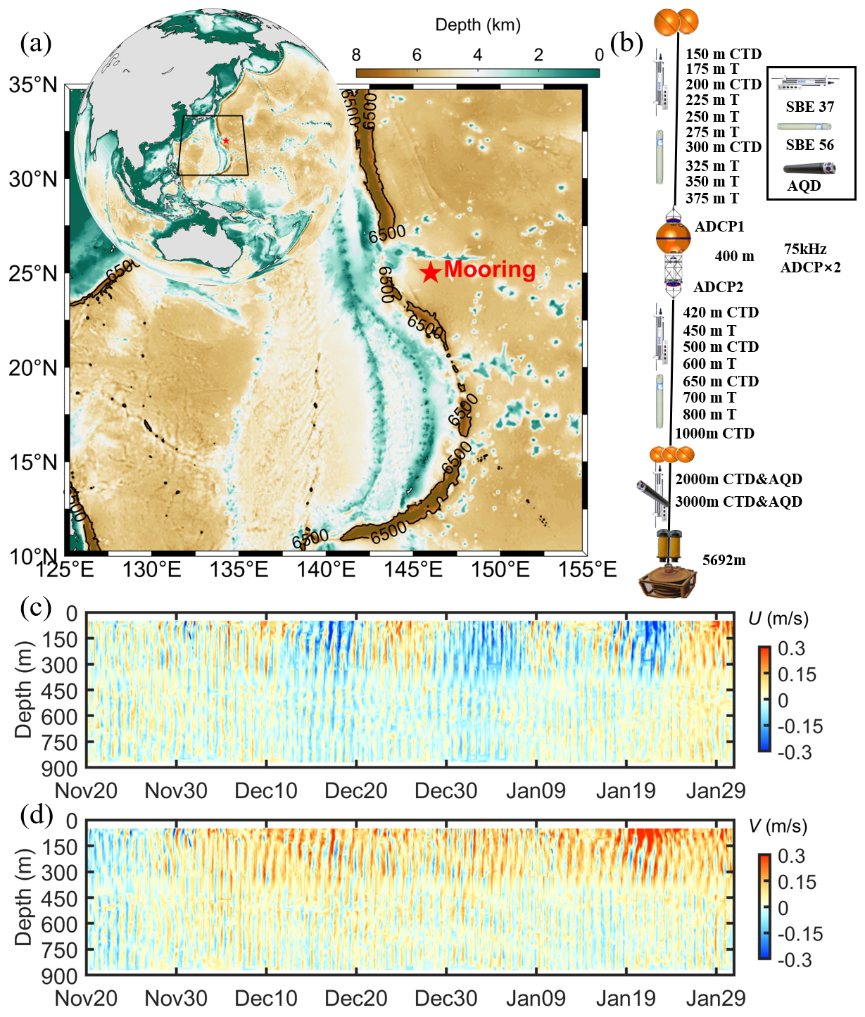
Figure 1 (a) Location of subsurface mooring (marked by a red pentagram), with color shading representing the topography. (b) Deployment depths of instruments on the subsurface mooring. (c, d) Depth-time plot of zonal and meridional velocities from 20 November 2017 to 31 January 2018.

Wind field data were obtained from the fifth major global reanalysis produced by the European Center for Medium-Range Weather Forecasts (ERA5). Thus, the wind stress vector, τ, and near-inertial velocity vector, v_ni, can be calculated via the parameterization of Oey et al. (2006) and the slab model of Pollard and Millard (1970) (with a damping parameter of 0.06 f₀), respectively. A comparison between the slab model derived near-inertial velocity and the observational near-inertial velocity is provided in Fig. S2. Sea level anomaly (SLA) and surface geostrophic velocity data were obtained from satellite altimetry products provided by Ssalto/Duacs and distributed through the Copernicus Marine Environment Monitoring Service (CMEMS).

Additionally, reanalysis data produced by the Met Office Coupled Atmosphere-Land-Ocean-Ice data assimilation (CPLDA) system were used to calculate the energy transfer rate between NIWs and mesoscale eddies. The product provides daily-averaged variables with a horizontal resolution of 0.25°×0.25°, including mixed layer depth, three-dimensional temperature, salinity, and currents. In the present study, the mixed layer depth (MLD) is defined as the depth where temperature is 0.5 °C lower than the sea surface temperature (Watanabe and Hibiya, 2002). This criterion was applied consistently throughout the present analysis. To verify the validity of using the reanalysis data, we compared them with the observational data. The results show that the reanalysis data agree well with the observations in variables of potential density and geostrophic currents (see Fig. S1 in the Supplement). Therefore, it is plausible to use reanalysis data to compute the energy transfer rate between NIWs and mesoscale eddies. Additionally, the World Ocean Atlas 2023 (WOA23) gridded climatological temperature and salinity fields were used to examine the modal decomposition of the near-inertial velocity field.

2.2 Modal decomposition

Vertical structure of internal waves can be represented by the superposition of multiple discrete baroclinic modes that only depend on the climatologic full-depth profile of stratification (D'Asaro et al., 1995; Fig. 2a and b). The vertical structure of each mode is constrained by (Gill, 1982; Thorpe and Jiang, 1998; Luo et al., 2024),

$$\begin{array}{}\text{(1)}& {\displaystyle \frac{{\partial }^{\mathrm{2}}{\mathrm{\Phi }}_n\left(z\right)}{\partial z^{\mathrm{2}}}}+{\displaystyle \frac{N^{\mathrm{2}}\left(z\right)}{c_n^{\mathrm{2}}}}{\mathrm{\Phi }}_n\left(z\right)=\mathrm{0}.\end{array}$$

The boundary conditions at sea surface and sea bottom are Φ_n(0)=0 and ${\mathrm{\Phi }}_n(-H)=\mathrm{0}$. Here, H is the water depth, n is the mode number, c_n is the eigenvalue, and N² is the buoyancy frequency square. Φ_n represents the baroclinic mode of vertical displacement. The corresponding baroclinic modes for the horizontal velocity are

$$\begin{array}{}\text{(2)}& {\mathrm{\Pi }}_n={\mathit{\rho }}_{\mathrm{0}}{c}_n^{\mathrm{2}}{\displaystyle \frac{\mathrm{d}{\mathrm{\Phi }}_n\left(z\right)}{\mathrm{d}z}}\end{array}$$

where ρ₀ is the reference density. The vertical profiles of the first five baroclinic modes for Φ_n and Π_n are shown in Fig. 2c and d. The horizontal near-inertial velocities can be expressed as

$$\begin{array}{}\text{(3)}& u(z,t)=\sum _{n=\mathrm{0}}^N{u}_n\left(t\right){\mathrm{\Pi }}_n\left(z\right).\end{array}$$

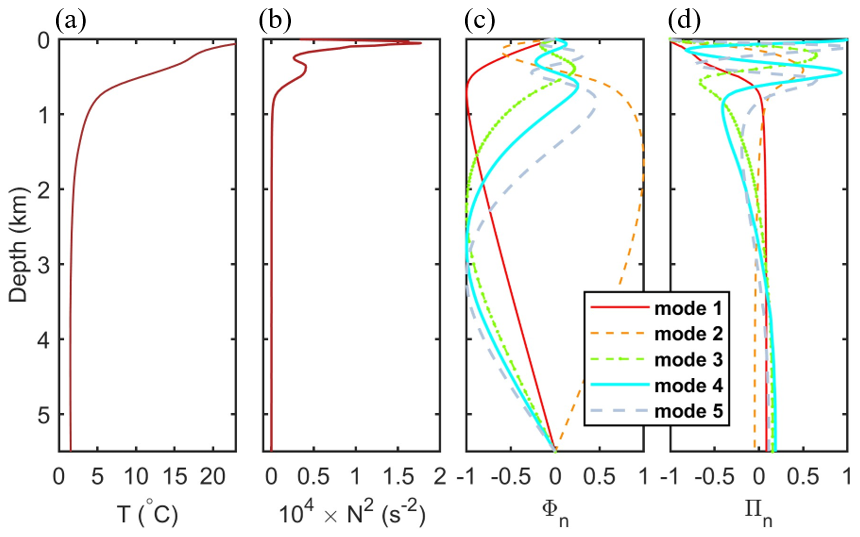
Figure 2 (a) Profile of potential temperature, T, from climatologic WOA23 data at the mooring site. (b) The same with (a), but for stratification N². (c) Normalized vertical structures of the first five baroclinic modes for vertical displacement. (d) The same as (c) but for horizontal velocity.

2.3 Energy transfer rate between mesoscale eddy and NIWs

Assuming that mesoscale eddies satisfy the geostrophic approximation, the corresponding energy transfer rate between mesoscale eddies and NIWs is given by Polzin (2010)

$$\begin{array}{}\text{(4)}& P=-\left(〈u_{\mathrm{ni}}{u}_{\mathrm{ni}}〉-〈v_{\mathrm{ni}}{v}_{\mathrm{ni}}〉\right){\displaystyle \frac{S_{\mathrm{n}}}{\mathrm{2}}}-〈u_{\mathrm{ni}}{v}_{\mathrm{ni}}〉S_{\mathrm{s}}\end{array}$$

where $S_{\mathrm{n}}=U_x-V_y$ and $S_{\mathrm{s}}=U_y+V_x$ represent the normal and shear components of the horizontal strain, respectively. Here, U and V are the background horizontal velocity fields obtained from the reanalysis product. A 5 d temporal low-pass filter was applied to the reanalysis velocity fields to obtain the background horizontal velocity. The zonal and meridional near-inertial velocities, u_ni and v_ni, were extracted using a fourth Butterworth band-pass filter over the frequency range of [0.9 1.1] f₀. The angular bracket denotes a smoothing average over three inertial periods. Sensitivity experiments using low-pass windows of 3, 5, 7 d and averaging windows of 2–4 inertial periods confirm that the sign and principal temporal evolution of P are robust to these parameter choices (Fig. S3).

2.4 Near-inertial ellipse analysis

Assuming that the observed NIWs are linear plane waves, the intrinsic frequency ω_i of NIWs satisfies a simplified dispersion relation (Cuypers et al., 2013),

$$\begin{array}{}\text{(5)}& {\mathit{\omega }}_{\mathrm{i}}^{\mathrm{2}}=f_{\mathrm{eff}}^{\mathrm{2}}+N^{\mathrm{2}}{\displaystyle \frac{k_{\mathrm{h}}^{\mathrm{2}}}{\left(m^{\mathrm{2}}+k_{\mathrm{h}}^{\mathrm{2}}\right)}},\end{array}$$

where f_eff is the effective Coriolis frequency, k_h is the horizontal wave number, m is the vertical wave number following Chen et al. (2023).

$$\begin{array}{}\text{(6)}& m=\partial \left(\mathrm{atan}\left(u_{\mathrm{ni}}/v_{\mathrm{ni}}\right)\right)/\partial z\end{array}$$

ω_i can be obtained by subtracting the Doppler shift from the observed frequency ω_o,

$$\begin{array}{}\text{(7)}& {\mathit{\omega }}_{\mathrm{i}}={\mathit{\omega }}_{\mathrm{o}}-\left|k_{\mathrm{h}}\right|\left|\mathit{V}\right|\cos (\mathrm{\Phi }-\mathit{\theta }),\end{array}$$

where Φ is the horizontal propagation direction of wave packets, V and θ represent the background velocity vector and direction of the mean current. V and θ are obtained from the mooring ADCP observations. By combining Eqs. (5) and (7), f_eff and k_h are given by (Alford and Gregg, 2001)

$$\begin{array}{}\text{(8)}& {\displaystyle }& {\displaystyle }{f}_{\mathrm{eff}}={\displaystyle \frac{{\mathit{\omega }}_{\mathrm{o}}}{\left(r+\frac{m\left|\mathit{V}\right|}{N}\cos (\mathrm{\Phi }-\mathit{\theta })\sqrt{r^{\mathrm{2}}-\mathrm{1}}\right)}},\text{(9)}& {\displaystyle }& {\displaystyle }{k}_{\mathrm{h}}^{\mathrm{2}}=m^{\mathrm{2}}\left({\mathit{\omega }}_{\mathrm{i}}^{\mathrm{2}}-f_{\mathrm{eff}}^{\mathrm{2}}\right)/N^{\mathrm{2}},\end{array}$$

where $r={\mathit{\omega }}_{\mathrm{i}}/f_{\mathrm{eff}}$ is the major to minor axis ratio of an inertial ellipse. The vertical group velocities are given by Cuypers et al. (2013),

$$\begin{array}{}\text{(10)}& c_{\mathrm{g}z}=-{\displaystyle \frac{\left(N^{\mathrm{2}}-f_{\mathrm{0}}^{\mathrm{2}}\right){\mathit{\beta }}^{\mathrm{3}}}{k_{\mathrm{h}}{\left(\mathrm{1}+{\mathit{\beta }}^{\mathrm{2}}\right)}^{\frac{\mathrm{3}}{\mathrm{2}}}{\left(f_{\mathrm{0}}^{\mathrm{2}}+N^{\mathrm{2}}{\mathit{\beta }}^{\mathrm{2}}\right)}^{\frac{\mathrm{1}}{\mathrm{2}}}}},\end{array}$$

where $\mathit{\beta }=k_{\mathrm{h}}/m$ is the angle of propagation to the vertical.

3 Results

3.1 Winter storms and wind-generated near-inertial energy into the mixed layer

According to the spatial and temporal distributions of wind fields, two wind storm events were identified during the observation period (Fig. 3). The first storm (hereafter called WS1) is from 6 to 18 December 2017, with the mean and maximum wind speeds of 8.5 and 13.8 m s⁻¹, respectively, at the subsurface mooring site. Another storm (hereafter called WS2) occurs between 6 and 17 January 2018. The second storm is weak relative to the first storm, with the mean and maximum wind speeds of 6.9 and 10.2 m s⁻¹, respectively. During the two storms, the wind speed and direction varied rapidly with time, thereby triggering corresponding near-inertial velocity responses in the mixed layer.

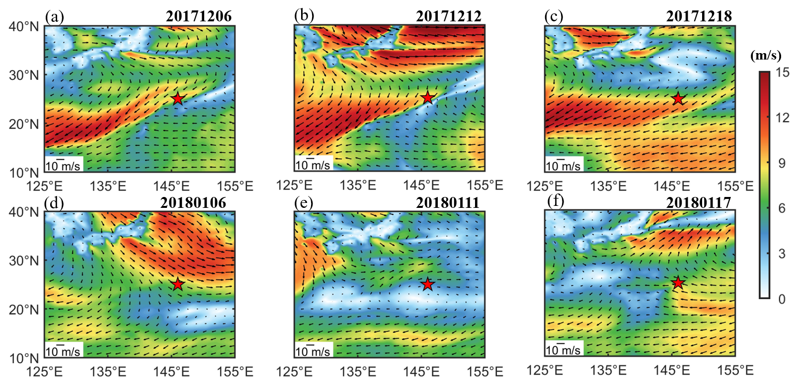
Figure 3 (a–c) Spatial and temporal distributions of wind speed from 6 to 18 December 2017, with arrows representing wind direction. (d–f) The same with (a)–(c), but corresponding to the distributions from 6 to 17 January 2018.

To illustrate the generation of NIWs at the subsurface mooring site, near-inertial velocity response and wind power input into the mixed layer calculated by a slab model are shown in Fig. 4a–c. Alford et al. (2012) observed that the near-inertial velocities in the mixed layer estimated from the slab model show a high agreement with observations. During WS1 and WS2, the generated near-inertial velocities in the mixed layer reach up to ∼0.6 and ∼0.2 m s⁻¹, respectively. The duration of strong near-inertial motions during WS1 is evidently longer than that during WS2. The mean wind power inputs into the mixed layer are $\mathrm{11.2}\times {\mathrm{10}}^{-\mathrm{3}}$ and $\mathrm{3.3}\times {\mathrm{10}}^{-\mathrm{3}}$ W m⁻² during WS1 and WS2, respectively. To compare the total wind-generated near-inertial energy input, the wind power is calculated cumulatively (Fig. 4d). The total near-inertial energy input into the mixed layer amounts to 11.5 kJ m⁻² during WS1 and 3.1 kJ m⁻² during WS2, respectively. Therefore, compared to the near-inertial energy input during WS2, the energy input during WS1 is approximately three times higher.

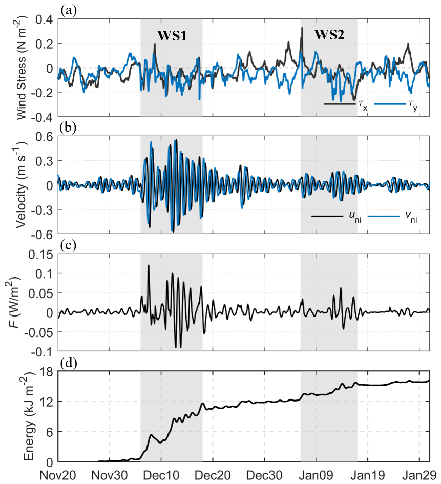
Figure 4 (a) Zonal (black line) and meridional (blue line) components of wind stress, (τ_x, τ_y), from 20 November 2017 to 31 January 2018. (b) Zonal and meridional near-inertial velocities, (u_ni, v_ni), calculated by a slab model. (c) Near-inertial energy flux, $F=\mathit{\tau }\cdot v_{\mathrm{ni}}$. (d) Cumulative near-inertial energy input into the mixed layer.

3.2 Observations of two energetic NIW events in winter

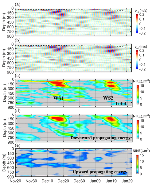
Figure 5a–c shows the observed near-inertial velocities and near-inertial kinetic energy ($\mathrm{NIKE}=\mathrm{0.5}\mathit{\rho }\times (u_{\mathrm{ni}}^{\mathrm{2}}+v_{\mathrm{ni}}^{\mathrm{2}})$, where ρ is a reference density). Corresponding to the passage of WS1 and WS2, two prominent near-inertial events are clearly resolved in observations. The first event occurs between 6 and 25 December 2017. Before 10 December, the near-inertial energy is confined above 80 m depth, followed by a rapid downward propagation before 20 December. At a depth of 120 m, near-inertial velocity and NIKE reach their maximum values, at 0.4 m s⁻¹ and 20 J m⁻³, respectively. The second event developed from 6 to 24 January 2018, during which the maximum near-inertial velocity and NIKE reach up to 0.21 m s⁻¹ and 21 J m⁻³ at a depth of 220 m, respectively. According to MacKinnon et al. (2013), the total near-inertial velocities are further processed by rotary decompositions to obtain downward propagating and upward propagating NIKE (Fig. 5d and e). Consistent with the general features of NIWs in the upper ocean, the total NIKE is dominated by the downward propagating component. According to Johnston et al., 2021, the value of one-tenth of the maximum NIKE was used as the criterion for energy propagation depth. The propagation depths for the two NIW events are basically comparable, both located at a depth of approximately 300 m (Fig. 5d). Additionally, the decay time is defined as the time required for the near-inertial energy to decrease from its maximum value to one-tenth of that value along the downward propagation path. Based on this method, the decay times are approximately 9 d for WS1 and 5 d for WS2.

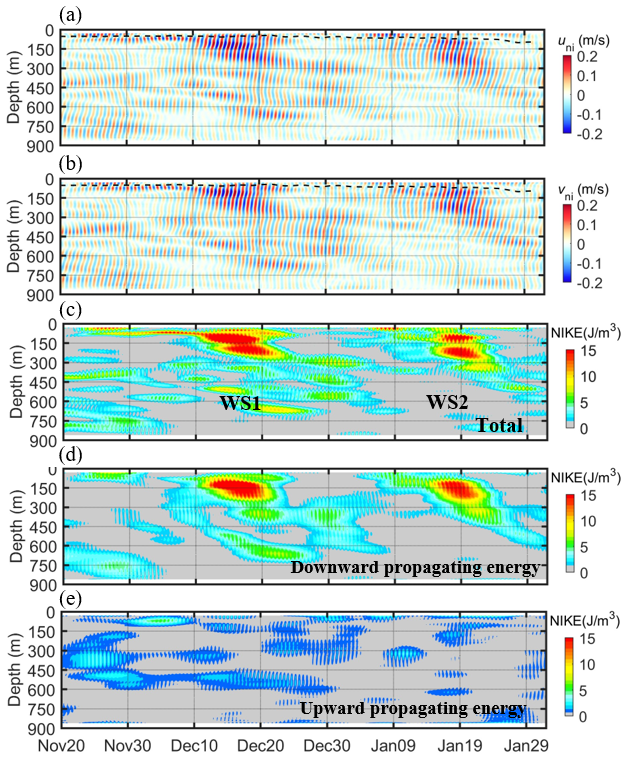
Figure 5 Depth-time plots of near-inertial velocities and near-inertial kinetic energy, NIKE, from 20 November 2017 to 30 January 2018. (a) Zonal near-inertial velocity, u_ni. (b) Meridional near-inertial velocity, v_ni. (c) Depth-time plot of NIKE. (d) and (e) are the same with (c), but for the downward-propagating and upward-propagating NIKE. The black dashed line in (a) and (b) indicates the mixed layer depth (MLD). The blue and brown circles in (c) indicate the time and depth of the maximum NIKE and one-tenth of the maximum NIKE for each NIW event, respectively.

It should be noted that although the wind-generated near-inertial energy input into the mixed layer during WS1 is about three times larger than that during WS2, the observed NIKE intensity is comparable (Figs. 4d and 5c). This means that during the downward propagation processes, additional energy may be transferred into the second NIW event or transferred out from the first NIW event. It will be further investigated in detail in the discussion section.

3.3 Characteristics of the two NIWs

According to Gonella (1972), rotary frequency spectra of raw velocities from ADCPs during the two winter storms are shown in Fig. 6. Relative to the diurnal and semidiurnal tides, near-inertial energy exhibits significant clockwise polarization. The near-inertial energy in clockwise polarization is approximately one to two orders of magnitude larger than that in counterclockwise polarization, consistent with the general characteristics of NIWs in the Northern Hemisphere. During the two wind storms, the near-inertial energy notably exceeds tidal energy, especially in the upper 300 m, dominating the energy within the internal wave spectrum. Additionally, the near-inertial frequency shows a red shift during WS2, indicative of the existence of positive relative vorticity or positive Doppler shift according to the frequency relationship (Kunze, 1985).

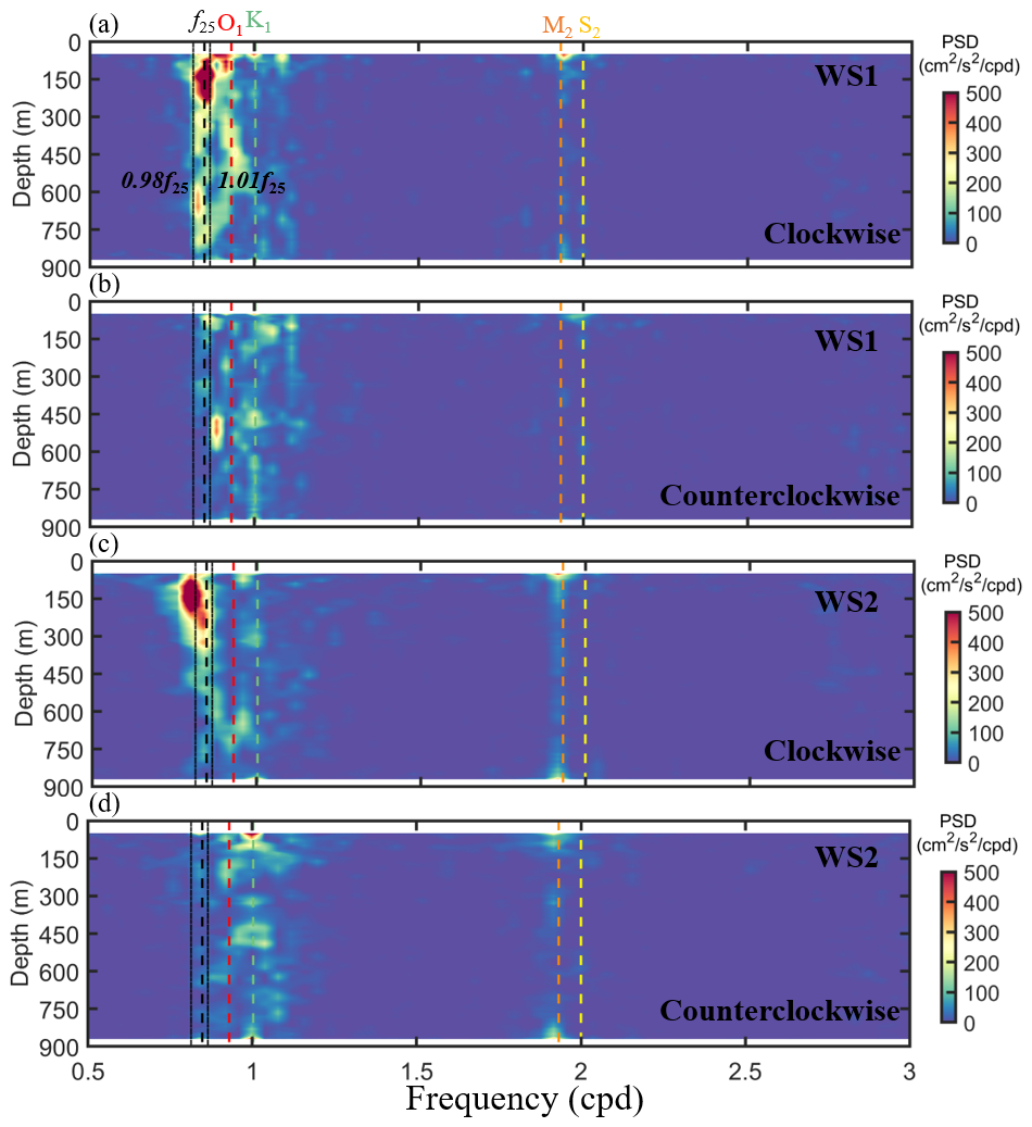
Figure 6 Rotary frequency spectra of raw velocities observed from ADCPs during WS1 (a, b) and WS2 (c, d). Clockwise and anticlockwise polarizations of velocities are shown in (a)–(d). The vertical dashed lines in panels represent the local inertial frequency, f₀, 0.98 f₀, 1.01 f₀, diurnal tidal frequency, O₁ and K₁, and semidiurnal tidal frequency, M₂ and S₂, respectively.

To further quantify the NIW properties during the two winter storms, the wavelengths, intrinsic frequency, and group velocities of the two near-inertial events are estimated by applying a near-inertial ellipse analysis (Fig. 7). Vertical wavelengths, λ_z, of NIWs can be estimated based on the vertical profiles of horizontal near-inertial velocities observed by ADCPs. For the two wave packets, their vertical wavelengths are 487 and 372 m, respectively. According to directions of ellipse major axis combined with directions of background horizontal velocity (Chen et al., 2024), the propagation direction of near-inertial packets can be determined. Through least squares fitting following Hebert and Moum (1994), the observed frequency is extracted from the two NIW packets, with values of 1.01 f₀ and 0.98 f₀, respectively. Then, substituting the above parameters into Eqs. (7)–(9) yields the effective Coriolis frequency, intrinsic frequency, and horizontal wavelength, λ_H. Based on Eq. (10), vertical group velocity can be determined. For the two wave packets, the mean vertical group velocity are 31.2 and 14.4 m d⁻¹, respectively, indicative of a slower vertical group velocity during WS2. Properties of the two wave packets are summarized in Table 1.

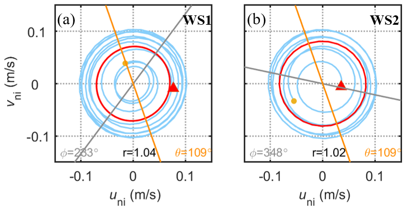
Figure 7 Depth-averaged near-inertial ellipses at the depth range of 70 to 300 m during WS1 and WS2. The brown dot and red triangle indicate the beginning and end of ellipse, respectively. The red ellipse is obtained from the least squares fitting following Hebert and Moum (1994). The gray and orange lines represent the mean directions of the NIW propagation, ϕ, and the background horizontal current, θ, respectively. The ratio of major axis to minor axis of the near-inertial ellipse, r, is indicated in the corresponding panel.

Table 1 Properties of the two NIW events. Errors (±) represent one standard deviation estimated from the corresponding internal wave parameters during each NIW event.

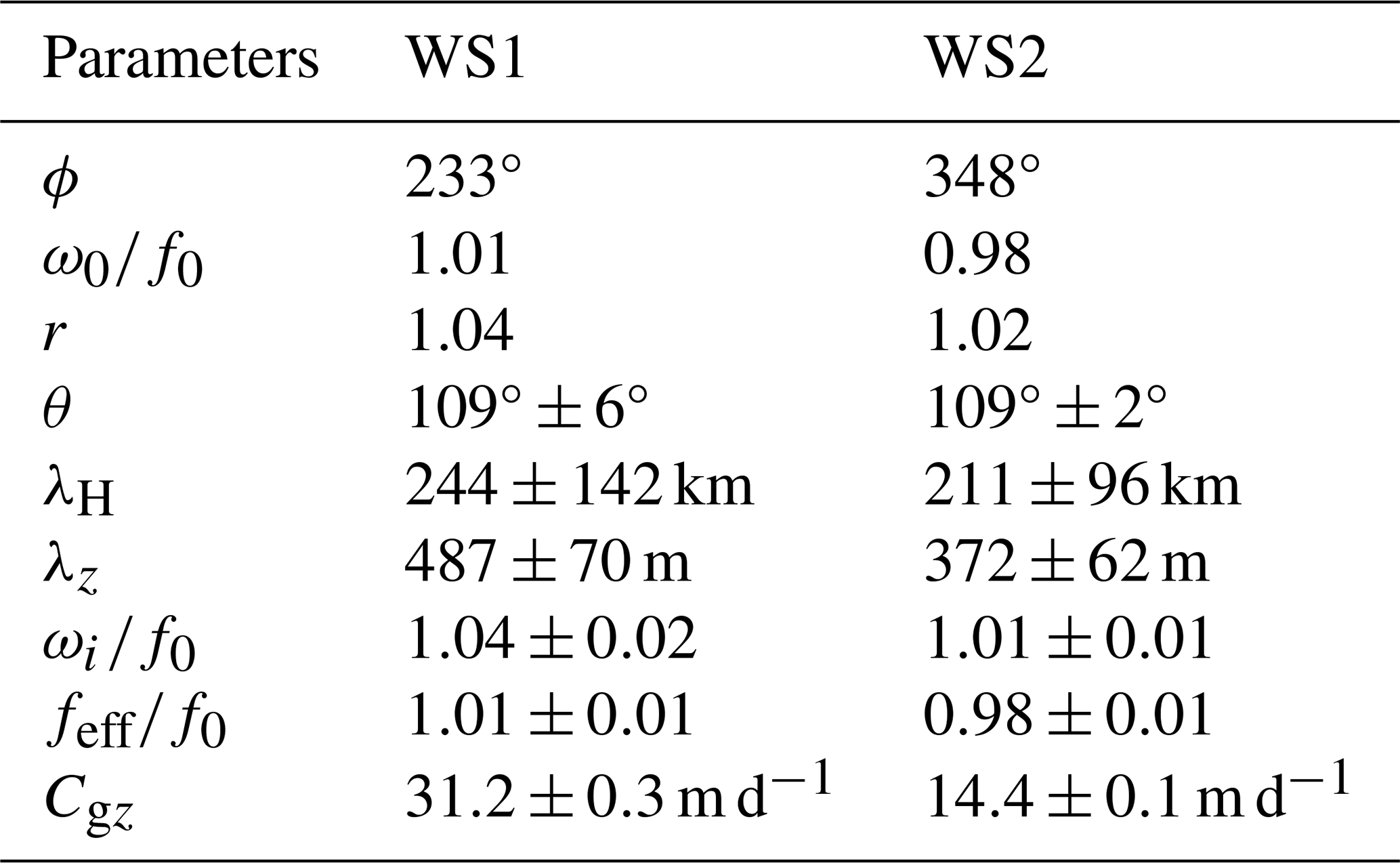
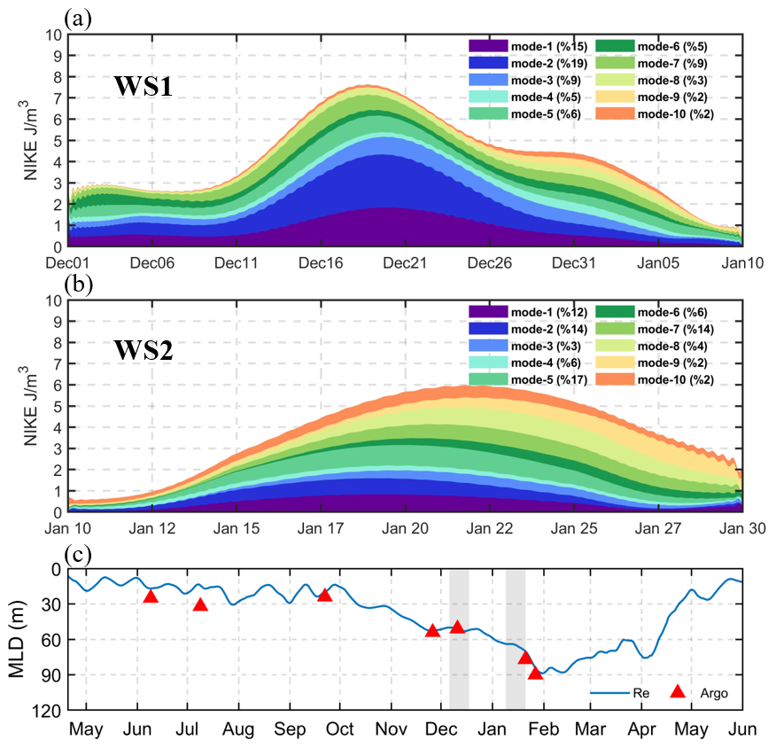
Figure 8 Depth-averaged near-inertial kinetic energy, NIKE, for the first 10 modes during WS1 (a) and WS2 (b). (c) Mixed layer depth during the full observational period calculated from reanalysis data (blue line), and Argo profiles (red triangles). Gray shading represents two storm events. Proportion of each mode's NIKE in the total NIKE is labeled in (a) and (b).

Next, the horizontal near-inertial velocities during WS1 and WS2 are projected onto the first 20 vertical baroclinic modes to investigate the modal characteristics of NIWs. Figure 8a and b shows the depth-averaged NIKE for the first 10 vertical baroclinic modes during WS1 and WS2, respectively. For the two NIW events, the NIKE in the first 10 modes accounted for 75 % and 80 % of the total NIKE, suggesting that the first 10 modes reconstructed the NIWs well. During WS1, the near-inertial energy is dominated by low modes, with the first four modes contributing 48 % of the total energy, while modes five to eight together account for only 24 %. In contrast to the modal content during WS1, the near-inertial energy during WS2 exhibits a characteristic dominated by high modal energy, with the fifth to eighth modes contributing 41 % of the total energy. Considering the difference in vertical wavelengths of the two NIW events, it is reasonable that the first NIW event with a larger vertical wavelength manifests a dominance of low modes. Correspondingly, the downward group velocity of the first wave packet is faster than that of the second wave packet.

Additionally, many previous researches suggest that the proportion of low modes in the total energy is correlated with MLD (Guthrie and Morison, 2021; Chen et al., 2025). In general, a shallow MLD shapes a short vertical wavelength of internal waves. However, as shown in Fig. 8c, the mean MLD during WS2 is approximately 70 m, which is deeper than that during WS1, with a depth of about 51 m. This is contrasted with the conventional expectation that deep mixed layer tends to favor a higher low-mode contribution. The discrepancy suggests that except for the MLD, other factors may be more important to control the modal content of the two NIW events. Further examination is discussed in Sect. 4.

4 Discussion

4.1 Energy exchange between mesoscale eddies and NIWs

To understand the comparable NIKE intensity observed in the thermocline despite discernible difference in cumulative wind-generated energy input into the mixed layer during the two winter storms, energy transfer rate between mesoscale eddies and NIWs is examined. Through energy exchange between low-frequency flows and internal waves, energy can be transferred both from low-frequency flows to internal waves and from internal wave to low-frequency flows, with the highest efficiency occurring between mesoscale eddies and NIWs (e.g., Polzin, 2010).

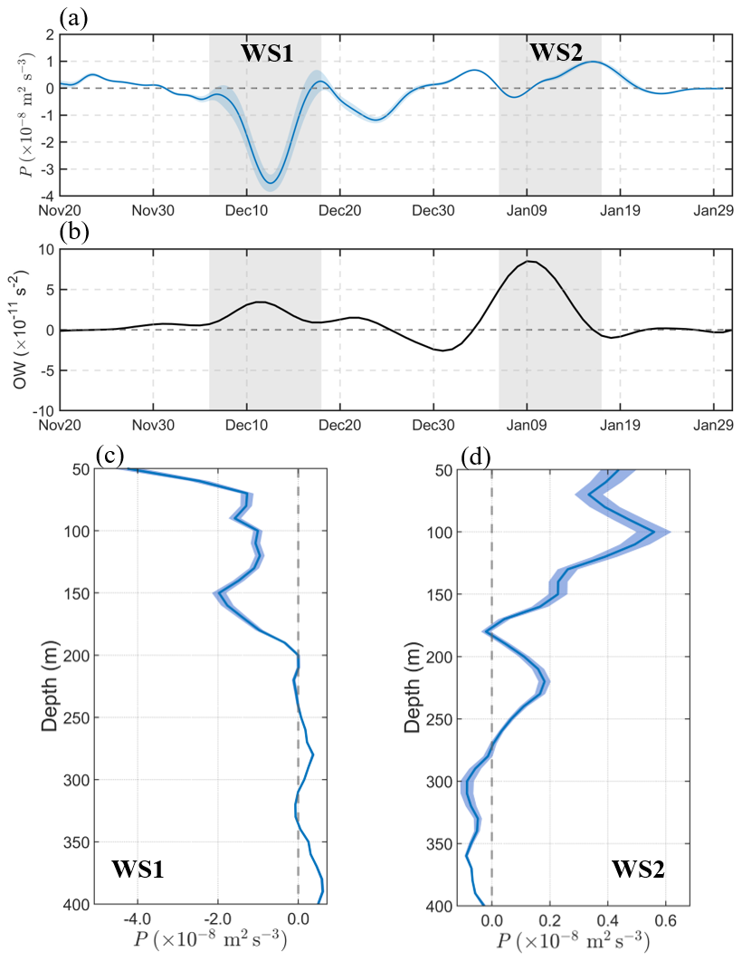
Figure 9 Energy exchange rate, P, between mesoscale eddies and NIWs. (a) Temporal variation of depth-averaged P within the mixed layer from 20 November 2017 to 31 January 2018. (b) Temporal variation of the Okubo–Weiss parameter, defined as $\mathrm{OW}=S_{\mathrm{n}}^{\mathrm{2}}+S_{\mathrm{s}}^{\mathrm{2}}-{\mathit{\zeta }}^{\mathrm{2}}$, where $S_{\mathrm{n}}=U_x-V_y$, $S_{\mathrm{s}}=V_x+U_y$ and $\mathit{\zeta }=V_x-U_y$. (c) Vertical profile of time-averaged P during WS1. (d) Vertical profile of time-averaged P during WS2. Blue shading in (a), (c), and (d) represents one standard deviation of the mean value.

Temporal variations of depth-averaged energy transfer rate between mesoscale eddies and NIWs within the mixed layer, P, are shown in Fig. 9a, with negative values indicating an energy transfer from near-inertial motions to the mesoscale eddies, and vice versa. P is permanently negative during WS1 and is basically positive during WS2. It suggests that the mesoscale eddy energy is transferred to near-inertial motions during WS2, while the opposite occurs during WS1. Additionally, the intensity of P during WS1 is considerably higher than that during WS2. Consistent with the findings of Jing et al. (2018), the strong P primarily occurs in period of positive OW parameter when strain dominates relative vorticity (Fig. 9b). Furthermore, vertical variations of the time-averaged P during WS1 and WS2 are shown in Fig. 9c and d, respectively, exhibiting significant energy transfer in the upper ∼200 m depth. The depth-averaged values of P during WS1 and WS2 are $-\mathrm{2.3}\times {\mathrm{10}}^{-\mathrm{8}}$ and $\mathrm{0.24}\times {\mathrm{10}}^{-\mathrm{8}}$ m² s⁻³, respectively.

Many studies suggest that approximately 25 % of wind-generated near-inertial energy in the mixed layer can radiate to the thermocline layer (e.g., Alford et al., 2012; Jing et al., 2018). Under this assumption, the two storms can generate near-inertial energy of approximately $\mathrm{2.8}\times {\mathrm{10}}^{-\mathrm{3}}$ and $\mathrm{0.82}\times {\mathrm{10}}^{-\mathrm{3}}$ W m⁻² into the thermocline layer during WS1 and WS2, respectively (Fig. 4). Considering that the enhanced NIKE associated with both NIW events is mainly distributed within the upper ∼300 m (Fig. 5c), the P is vertically integrated over the upper 300 m. After vertically integrating of P in the upper 300 m, $\underset{\mathrm{300}}{\overset{\mathrm{0}}{\int }}\mathit{\rho }P\mathrm{d}z$, the energy exchange between mesoscale eddies and NIWs is $-\mathrm{1.3}\times {\mathrm{10}}^{-\mathrm{3}}$ W m⁻² during WS1 and $\mathrm{0.36}\times {\mathrm{10}}^{-\mathrm{3}}$ W m⁻² during WS2, respectively. Thus, approximately 46 % of the wind-generated near-inertial energy is converted into mesoscale eddy during WS1. However, mesoscale eddies contribute approximately 43 % of the wind-generated near-inertial energy to NIWs during WS2. Combining the wind energy input and mesoscale eddy's energy transfer, the remaining near-inertial energy input is approximately $\mathrm{1.5}\times {\mathrm{10}}^{-\mathrm{3}}$ W m⁻² during WS1 and $\mathrm{1.2}\times {\mathrm{10}}^{-\mathrm{3}}$ W m⁻² during WS2.

Furthermore, the time-integrated energy was calculated to compare the cumulative energy contribution over the two NIW events. The time-integrated wind-generated near-inertial energy flux, ∫Fdt, is 2.9 and 0.8 kJ m⁻² for WS1 and WS2, respectively. The time-integrated energy transfer, ∬ρPdzdt, is −1.3 and 0.5 kJ m⁻², respectively. This indicates that mesoscale eddies remove a substantial fraction of wind-generated near-inertial energy in WS1, whereas they provide an additional energy source for NIWs in WS2. These estimates indicate that the eddy-wave interactions reduce the difference between NIKE in WS1 and WS2 and may therefore contribute to the comparable observed NIKE. Note that the background velocity in reanalysis data is systematically higher than that in observational data (Fig. S1a and b). Therefore, an overestimation of background horizontal velocity in reanalysis data may introduce uncertainties in the calculation of strains and the eddy-NIW energy transfer.

4.2 Energy loss through turbulent dissipation and untrapped waves

The analysis above focuses on the energy exchange between mesoscale eddies and NIWs. However, near-inertial energy may also be influenced by other pathways, including turbulent dissipation and the radiation of untrapped waves away from the observation site. Because direct turbulence measurements were not available, we could not directly quantify turbulent dissipation from microstructure observations. Instead, we estimated the parameterized dissipation rate using the Gregg–Henyey–Polzin (GHP) parameterization based on the observed velocity and stratification fields (Henyey et al., 1986; Gregg, 1989; Kunze et al., 2006; Polzin et al., 2014). Details of the implementation, including the spectral calculation and parameter choices, are provided in Sect. S4. It should be noted that the GHP estimate reflects the dissipation associated with the internal wave shear and therefore includes contributions from NIWs, diurnal tides, and semidiurnal tides.

The time-averaged dissipation rates during WS1 and WS2 are $\mathrm{3.9}\times {\mathrm{10}}^{-\mathrm{10}}$ and $\mathrm{5.0}\times {\mathrm{10}}^{-\mathrm{10}}$ m² s⁻³, respectively (Fig. 10a). The corresponding time-integrated energy dissipation values are $\mathrm{4.1}\times {\mathrm{10}}^{-\mathrm{4}}$ and $\mathrm{4.3}\times {\mathrm{10}}^{-\mathrm{4}}$ m² s⁻², respectively. These comparable values indicate that turbulent dissipation was of similar magnitude during the two NIW events. Moreover, the estimated dissipation rates are approximately one order of magnitude smaller than the wind energy input and the mesoscale eddy-NIW energy exchange. Therefore, despite uncertainties associated with the parameterization, turbulent dissipation is unlikely to be a dominant pathway controlling the NIKE evolution during WS1 and WS2.

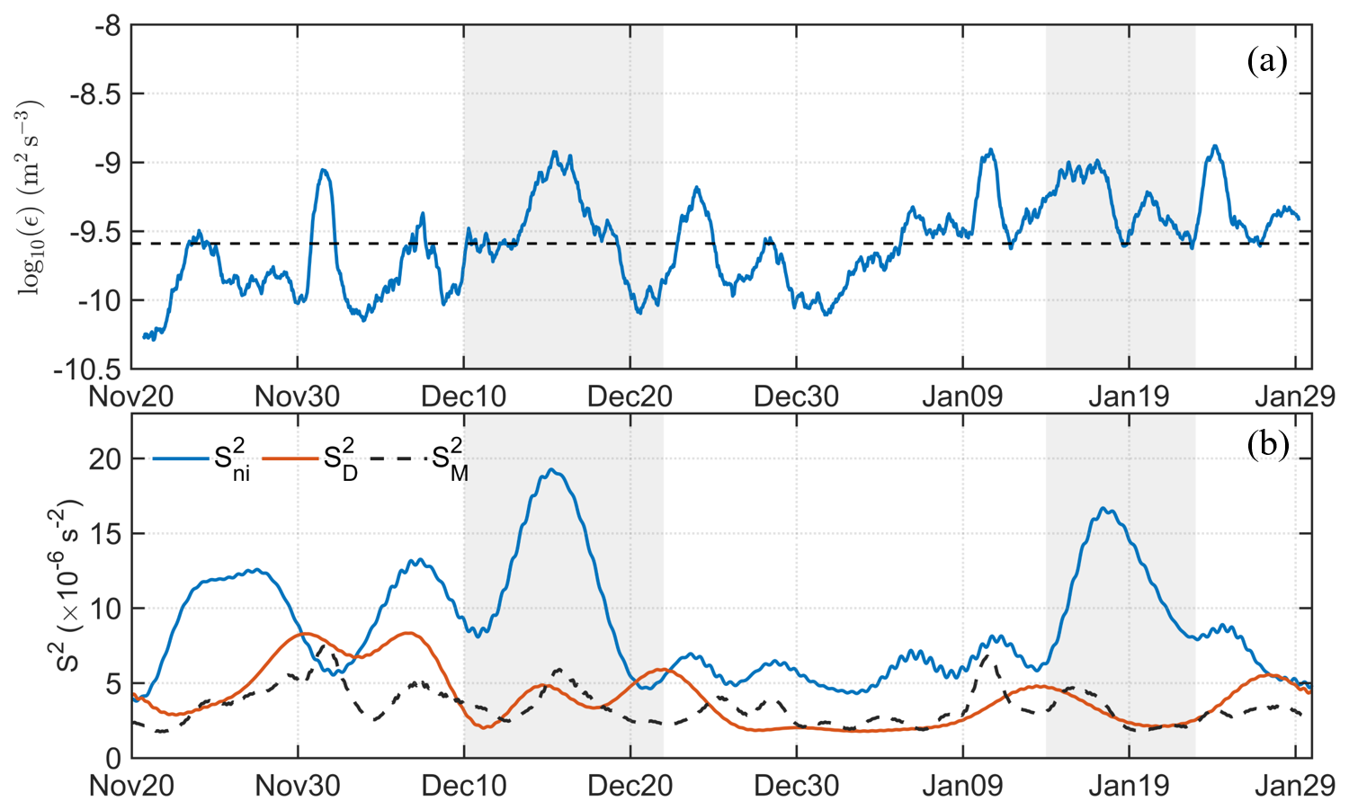
Figure 10 (a) Time series of the turbulent dissipation rate from GHP parameterization, during the observational period (50–300 m). The gray shading indicates the two NIW events. The horizontal dashed line denotes the time-averaged value. (b) Time series of vertical shear variance of near-inertial, diurnal, and semidiurnal components.

To further identify the dominant shear component of internal waves, the total vertical shear was decomposed into the near-inertial, diurnal and semidiurnal components. The corresponding vertical shear variances were calculated as $S_{\mathrm{ni}}^{\mathrm{2}}={\left|\partial u_{\mathrm{ni}}/\partial z\right|}^{\mathrm{2}}+{\left|\partial v_{\mathrm{ni}}/\partial z\right|}^{\mathrm{2}}$, $S_{\mathrm{D}}^{\mathrm{2}}={\left|\partial u_{\mathrm{D}}/\partial z\right|}^{\mathrm{2}}+{\left|\partial v_{\mathrm{D}}/\partial z\right|}^{\mathrm{2}}$, and $S_{\mathrm{M}}^{\mathrm{2}}={\left|\partial u_{\mathrm{M}}/\partial z\right|}^{\mathrm{2}}+{\left|\partial v_{\mathrm{M}}/\partial z\right|}^{\mathrm{2}}$, where $S_{\mathrm{ni}}^{\mathrm{2}}$, $S_{\mathrm{D}}^{\mathrm{2}}$, and $S_{\mathrm{M}}^{\mathrm{2}}$  epresent the near-inertial, diurnal, and semidiurnal shear variances, respectively. The mean near-inertial shear variances during WS1 and WS2 are approximately three to four times larger than those of diurnal and semidiurnal components (Fig. 10b). This dominance of near-inertial shear suggests that near-inertial motions play a major role in enhancing the total shear and the associated dissipation rate during the two storm events.

In addition to turbulent dissipation, the radiation of untrapped waves may also contribute to the loss of locally observed near-inertial energy. The modal analysis shows that WS1 is characterized by a higher contribution from low modes, whereas WS2 contains a larger proportion of high-mode energy (Fig. 8a and b). Low-mode NIWs are generally more efficient at propagating away from their generation region, while high-mode NIWs are more likely to generate strong local shear and dissipate locally. Thus, near-inertial energy during WS1 may exhibit stronger outward propagation compared to that during WS2. However, the outward radiation of near-inertial energy cannot be quantitatively evaluated from a single subsurface mooring.

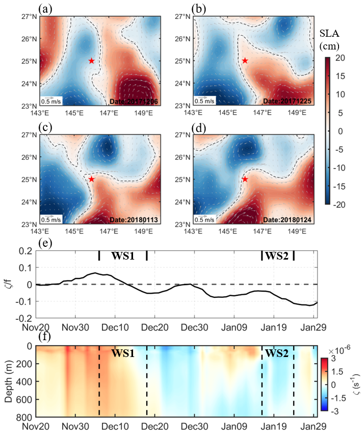
Figure 11 (a–d) Temporal-spatial distributions of sea level anomaly, SLA, with arrows indicating geostrophic currents. The red star represents the position of the subsurface mooring. (e) Temporal variation of relative vorticity calculated from surface geostrophic currents. (f) Depth-time distribution of relative vorticity derived from the reanalysis product.

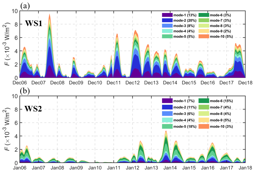
Figure 12 Temporal variation of wind-generated near-inertial energy flux, F, projected onto the first 10 modes during WS1 (a) and WS2 (b).

4.3 Roles of eddies and wind work modes in the NIW modal content

By analyzing the characteristics of NIWs, the modal content of NIWs during WS1 and WS2 is associated with the vertical wavelengths of NIWs. A large vertical wavelength corresponds to the dominance of low modes in NIWs. During the downward propagation of NIWs, the vertical wavelength is modulated by the relative vorticity of mesoscale eddies (D'Asaro et al., 1995; Kunze, 1985; Chen et al., 2026). The vertical variation of relative vorticity below the sea surface cannot be estimated directly from our observations. However, it is acknowledged that the relative vorticity increases with increasing depth in an anticyclonic eddy (ACE) and decreases with depth in a cyclonic eddy (CE). Thus, when NIWs are generated in an ACE, the increasing relative vorticity with depth can reduce the vertical wavelength of NIWs, resulting in the elimination of vertical group velocity and the formation of critical depth of NIWs (Kunze, 1985). Moreover, when NIWs propagate into an ACE from a region with positive relative vorticity, the relative vorticity gradually decreases along the propagation trajectory of NIWs, resulting in the increase of vertical wavelength (Chen et al., 2023). As shown in Fig. 11a–e, the relative vorticity gradually decreases from positive to negative due to a westward-moving ACE passing over the subsurface mooring site during WS1. The depth-time distribution of relative vorticity derived from the reanalysis product is consistent with the surface vorticity, with positive to negative vorticity during WS1 and predominantly negative vorticity during WS2 (Fig. 11f). Therefore, during WS1, the vertical wavelength of NIWs can gradually increase, subsequently leading to the dominance of low modes in NIWs. However, the relative vorticity is negative during WS2, consequently reducing the vertical wavelength and favoring the dominance of high modes in NIWs (Zheng et al., 2023b).

Additionally, differences in modal projection of wind-generated near-inertial energy flux may also contribute to the difference in NIW modal content during WS1 and WS2. Following the modal decomposition method of Raja et al. (2022), the wind-generated near-inertial energy flux is projected onto the first 20vertical baroclinic modes, $F_n\left(t\right)=\mathit{\tau }\left(t\right)\cdot v_{\mathrm{ni},n},$ where τ is the wind stress vector and v_ni,n is the nth-mode near-inertial velocity at 50 m depth. Figure 12 shows the temporal variation of wind-generated near-inertial energy flux in the first 10 modes. During WS1, the first four modes account for 50 % of the total wind-generated near-inertial energy input, while modes five to eight together account for only 14 %. However, during WS2 the fifth to eighth modes contribute 41 % of the total wind-generated near-inertial energy input, indicating that wind forces exert a larger projection onto higher modes. Therefore, the discrepancies of modal content in the two NIW events could be interpreted as the joint result of the modal projection of wind-generated near-inertial energy and modulation by mesoscale eddies.

5 Summary

In this study, the generation and downward propagation characteristics of two NIW events during winter storms are examined using subsurface mooring observations combined with reanalysis data. Wind-generated near-inertial energy input suggests that the energy input into the mixed layer during WS1 is approximately three times higher than that during WS2, but the observed NIKE is comparable between the two events. The energy exchange between mesoscale eddies and NIWs indicates that approximately 46 % of the wind-generated near-inertial energy is converted into mesoscale eddy during WS1, whereas mesoscale eddies contribute approximately 43 % of the wind-generated near-inertial energy to NIWs during WS2. The eddy-wave energy transfers may contribute to the comparable observed NIKE during the two events. However, turbulent dissipation and the radiation of energy out of the observed volume may also contribute to the comparable observed NIKE and cannot be fully quantified using the single mooring observations.

For the two NIW events, both the decay time, vertical wavelength, vertical group velocity of the first wave packet are larger than those of the second wave packet. Correspondingly, the first wave packet is dominated by low modes, while the second wave packet exhibits a characteristic of high mode dominance. The first four modes contribute 48 % of the total near-inertial energy in the first NIW event. However, 41 % of near-inertial energy is projected onto the fifth to eighth modes during WS2. It is found that modulation of eddies and modal content of wind-generated near-inertial energy input are of importance in determining the characteristics of modal content during the two NIW events. These findings highlight the combined roles of wind forcing and mesoscale eddy modulation in shaping energetic NIWs and have important implications for understanding wintertime interior mixing driven by breaking NIWs. Nevertheless, the analysis was based on observations from a single mooring site, which may not fully capture the spatial variability of NIW dynamics and their interaction with mesoscale structures across the broader region. Therefore, more observations and numerical studies on the dynamic characteristics of NIWs are needed in the future.