Chlorophyll a concentration effects on equatorial Atlantic Ocean mean-state and interannual variability

Chlorophyll a concentration is known to influence the mean-state and interannual sea surface temperature (SST) variability of the tropics. Here, we investigate this effect in the equatorial Atlantic Ocean using a suite of ocean model simulations. In these simulations, the prescribed monthly climatology of chlorophyll a concentration is multiplied by a factor ranging from 0.01 to 2. We find that a “clear-ocean” simulation, i.e an ocean simulation with the monthly climatology of chlorophyll a concentration multiplied by 0.01, results in a significantly warmer (+0.15 °C) eastern equatorial Atlantic SST and in a reduced (14 %) amplitude of SST seasonal cycle when compared against a simulation with realistic chlorophyll a levels. Additionally, the vertical temperature gradient around the main oceanic thermocline of the equatorial Atlantic is weakened, the mixed layer and main oceanic thermocline are deepened, and the equatorial upwelling across the mixed-layer base is reduced. These changes in the mean-state of the “clear-ocean” simulation lead to a significant reduction (12.9 %) in eastern equatorial Atlantic SST variability. We also show that when the prescribed monthly climatology of chlorophyll a concentration is scaled by 0.01, 0.5, 1, 1.5, and 2, the eastern equatorial Atlantic SST variability responds non-linearly, decreasing more strongly under low chlorophyll a concentrations than it increases under comparable high chlorophyll a conditions. Our results also suggest that the ongoing observed decrease in tropical Atlantic chlorophyll a concentration may weaken the interannual variability of SST.

1 Introduction

The tropical Atlantic Ocean exhibits a marked interannual sea surface temperature (SST) variability driven by the Atlantic zonal mode, also called Atlantic Niño (Zebiak, 1993; Lübbecke et al., 2018; Richter and Tokinaga, 2021). Atlantic Niños (Niñas) are extreme warm (cold) events characterized by large deviations from the seasonal cycle and typically occurring during May–June–July in the eastern equatorial Atlantic (ATL3 region; 3° S–3° N, 20° W–0° E). In addition, a secondary peak in interannual SST variability is observed in November–December, referred to as Atlantic Niño II (Okumura and Xie, 2006). The dynamics associated with the Atlantic Niño share similarities with the El Niño-Southern Oscillation (ENSO) in the Pacific Ocean (Servain et al., 1982; Keenlyside and Latif, 2007). Both climate modes involve a coupling of SST anomalies, zonal wind stress, and ocean heat content as described by the Bjerknes feedback loop (Bjerknes, 1969).

Atlantic Niños/Niñas can affect the climate of the neighboring continents (Hirst and Hastenrath, 1983), for example by modifying the onset of the West African Monsoon (Caniaux et al., 2011; Brandt et al., 2011) or influencing the Indian Monsoon (Kucharski et al., 2008). These events can also impact local marine ecosystems (Grodsky et al., 2008; Chenillat et al., 2021) as well as the sea-air CO₂ flux (Koseki et al., 2023). Therefore, enhancing our understanding of the Atlantic Niño mode, and its future evolution, is of particular socio-economic importance.

Atlantic Niños/Niñas occur in the equatorial Atlantic upwelling system (Brandt et al., 2023), which is rich in phytoplankton. Phytoplankton are aquatic photosynthetic organisms that form a crucial component of the global biogeochemical system and the basis of the marine food chain. Their presence in the water column affects the absorption of shortwave radiation, thereby influencing the vertical distribution of shortwave heating in the upper ocean (Lewis et al., 1990). Changing water clarity in coupled model simulations has been shown to result in significant changes in the global climate and circulation (Gnanadesikan and Anderson, 2009). Chlorophyll a concentration (Chl a hereafter) is typically used as a proxy for phytoplankton because it is the primary pigment involved in the photosynthesis of phytoplankton. In addition, Chl a is accurately and easily measured by satellites (Yoder and Kennelly, 2003), and it has been used to parameterize the effect of phytoplankton on solar radiation absorption in ocean and coupled models (Lewis et al., 1990; Morel and Antoine, 1994; Manizza et al., 2005). The impact of this effect on the mean-state and interannual variability of the tropical Pacific Ocean has been examined in observations (Strutton and Chavez, 2004) and extensively studied using ocean model experiments (Nakamoto et al., 2001; Murtugudde et al., 2002; Manizza et al., 2005; Sweeney et al., 2005; Park et al., 2014a, b) as well as coupled ocean-atmosphere-biogeochemistry models (Lengaigne et al., 2007; Anderson et al., 2009; Park et al., 2014a, b). However, despite the number of studies, the results remain somewhat contradictory (a summary can be found in Park et al., 2014b). Some studies find an increase in eastern equatorial Pacific SST in the presence of Chl a (Murtugudde et al., 2002; Marzeion et al., 2005), whereas others found a decrease (Manizza et al., 2005; Sweeney et al., 2005; Nakamoto et al., 2001; Löptien et al., 2009; Anderson et al., 2007, 2009; Jochum et al., 2010). Similarly, there is no consensus regarding the response of ENSO variability to the presence of Chl a: it may either amplify ENSO (Marzeion et al., 2005; Lengaigne et al., 2007; Löptien et al., 2009; Anderson et al., 2009; Park et al., 2014a, b) or dampen it (Timmermann and Jin, 2002; Wetzel et al., 2006; Jochum et al., 2010).

The effects of this bio-physical process have received less attention in the tropical Atlantic Ocean, although the seasonal cycle of Chl a in the eastern equatorial Atlantic is more pronounced than that of the eastern equatorial Pacific (Brandt et al., 2025). Frouin et al. (2007) compared an ocean general circulation model with constant Chl a of 0.02 mg m⁻³ to a simulation with time and spatially varying Chl a. They found in the simulation with varying Chl a a cooling in the northern part of the Benguela upwelling system, an enhanced Equatorial Undercurrent and strengthened Benguela Current, as well as an increased meridional circulation in the upper 50 m and a decrease below 50 m. Similarly, Hernandez et al. (2017) compared a regional ocean model configuration with a constant and horizontally homogeneous Chl a of 0.05 mg m⁻³, i.e. depleted water, to a simulation with a realistic monthly climatology of Chl a. They found that relative to the low Chl a simulation, the realistic simulation featured a cooling in the eastern equatorial Atlantic as well as in the Benguela and Senegalo–Mauritanian upwelling systems. Yet, to our knowledge the response of the interannual SST variability to the presence of Chl a has not yet been examined in the equatorial Atlantic.

Here, we aim to investigate the equatorial Atlantic interannual SST variability response to this bio-physical process through ocean model experiments forced with different scaling factors applied to the same monthly Chl a climatology. Specifically, this study addresses the following questions: 1) What are the effects of Chl a on the mean-state of the equatorial Atlantic Ocean? 2) How would interannual SST variability in the equatorial Atlantic respond if Chl a were nearly zero, halved or doubled?

To explore these questions, we present the different datasets, model configuration, and strategy used in Sect. 2. In the tropical Atlantic, the interannual SST variability is linked to the mean state. Therefore, we first examine the response of the tropical Atlantic mean-state to varying monthly climatology of Chl a in Sect. 3.1. Then, we investigate the equatorial Atlantic interannual SST variability response to the presence of Chl a in Sect. 3.2. Finally, we provide a summary and a discussion of the main results in Sect. 4.

2 Data and methods

2.1 Observational data

The monthly mean SST data from the Optimum Interpolation SST version 2.1 Reynolds et al. (2007, OI-SST), produced by the Physical Sciences Laboratory of the National Oceanic and Atmospheric Administration (NOAA), are used as a reference dataset to validate the seasonal cycle of SST and of SST variability of the control run (introduced in the next section) and to compare with the ones from the different sensitivity experiments. These data are available at 0.25° horizontal resolution from September 1981 to present day. Monthly means of Chl a, derived from the daily gap-free product Copernicus-GlobColour (Copernicus, 2024), are used to compute the linear trend in Chl a pointwise in the tropical Atlantic for the period 1998–2024. This product is available at 4 km horizontal resolution from 4 September 1997 to present day.

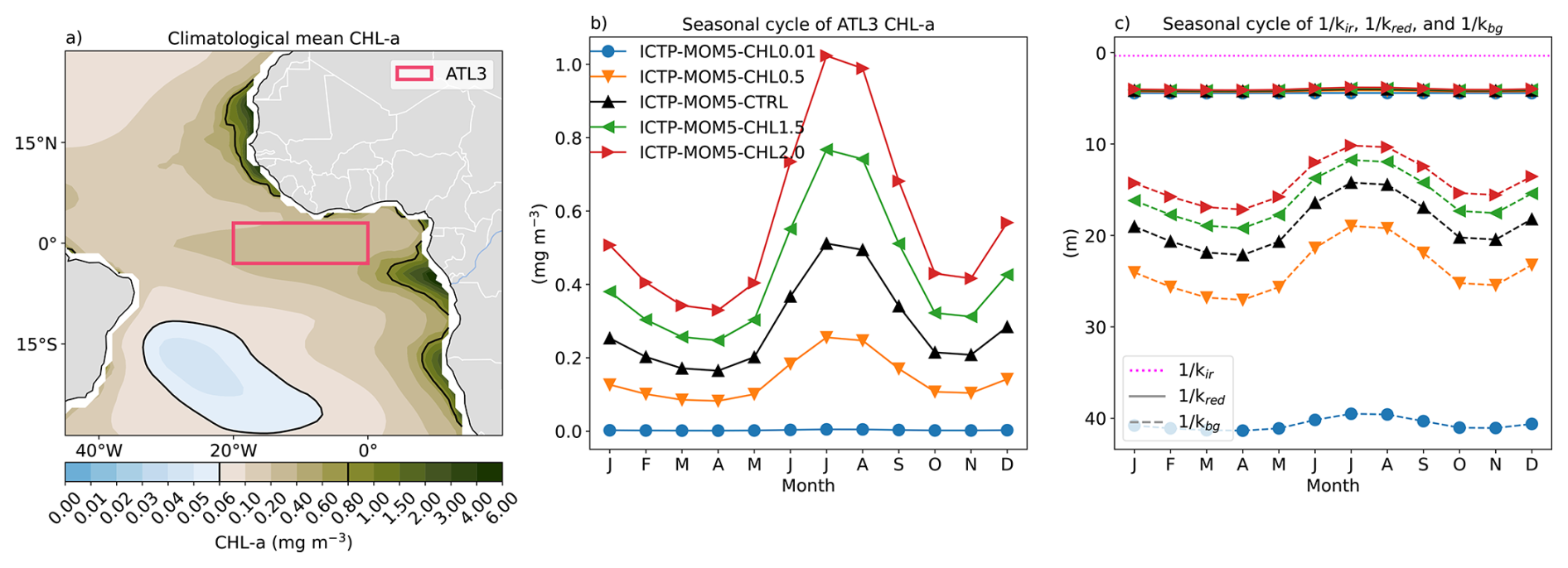
Figure 1 (a) Climatological mean Chl a concentration prescribed to ICTP-MOM5-CTRL. Black contours indicate the 0.06 and 0.80 mg m⁻³ Chl a concentration levels. (b) Seasonal cycle of the prescribed Chl a concentration averaged over the ATL3 (3° S–3° N, 20° W–0° E) region and for the different model simulations: ICTP-MOM5-CHL0.01 (blue), ICTP-MOM5-CHL0.5 (orange), ICTP-MOM5-CTRL (black), ICTP-MOM5-CHL1.5 (green), and ICTP-MOM5-CHL2.0 (red). (c) Seasonal cycles of the e-folding depth scales of the light penetration in the ATL3 region for the infrared ($\mathrm{1}/k_{\text{ir}}$, magenta dotted line), the red ($\mathrm{1}/k_{\text{red}}$, full lines), and the blue/green ($\mathrm{1}/k_{\text{bg}}$, dashed lines) wavelength bands. As $\mathrm{1}/k_{\text{red}}$ and $\mathrm{1}/k_{\text{bg}}$ depend on the Chl a concentration (cf. Eqs. 2 and 3), the seasonal cycles are plotted for each model experiment.

2.2 Ocean model configuration and experiments

To investigate the effect of Chl a on the equatorial Atlantic Ocean mean-state and its interannual variability, the NOAA-Geophysical Fluid Dynamics Laboratory Modular Ocean Model version 5 Griffies (2012, MOM5) was used. MOM5 is a free-surface primitive-equation model and uses z* rescaled geopotential coordinate. The model configuration for the control run (ICTP-MOM5-CTRL) corresponds to: 1° horizontal resolution with 50 vertical levels, subgrid mesoscale processes are parametrized with the Gent–McWilliams skew-flux closure scheme (Gent and Mcwilliams, 1990; Gent et al., 1995; Griffies, 1998) and submesoscale eddy fluxes according to Fox-Kemper et al. (2008, 2011). Vertical mixing is represented with a K-profile parameterization (Large et al., 1994). The control run was integrated from January 1958 to December 2021 using the JRA-55-based surface dataset for driving ocean-sea-ice models Tsujino et al. (2018, JRA55-do). Additionally, ICTP-MOM5-CTRL includes a monthly climatology of Chl a, which is based on 8 d composites of Sea-viewing Wide Field-of-view Sensor (SeaWiFS) images taken from 1999 to 2001. This is the baseline climatology used across all sensitivity experiments described in the following. The climatological mean field of this dataset is shown in Fig. 1a. More details on the production of this climatology can be found in Griffies (2012).

A caveat of forced ocean-sea ice configurations is the lack of two-way ocean–atmosphere coupling. In ICTP-MOM5, the ocean model is forced with the time-evolving JRA55-do atmospheric state, including winds at 10 m, shortwave and longwave heat fluxes, and near-surface (2 m) atmospheric temperature and humidity, which are used to calculate latent and sensible heat fluxes through bulk formulae. This forcing enables the model to realistically reproduce historical oceanic conditions over the simulation period. Additionally, the absence of SST restoring, together with the weak sea surface salinity restoring, prevent the artificial damping of intrinsic ocean variability. Nevertheless, prescribing the near-surface atmospheric state imposes some constraints on the simulated SST through the turbulent heat fluxes. Despite this limitation, Park et al. (2014b) showed that the impact of Chl a on the eastern tropical Pacific SST is qualitatively consistent between ocean-only and fully-coupled model experiments. Their results indicate that atmosphere-ocean coupling mostly amplifies the Chl a-induced mean change through a positive atmosphere feedback, but does not change the sign of the response. Moreover, the simulated response of ENSO in both fully-coupled and ocean-only model experiments was consistent (Park et al., 2014b). These findings suggest that forced ocean simulations provide a robust framework for investigating the influence of Chl a on the equatorial Atlantic variability. Yet, we acknowledge that the magnitude of the response may be lower than if a fully coupled system was considered.

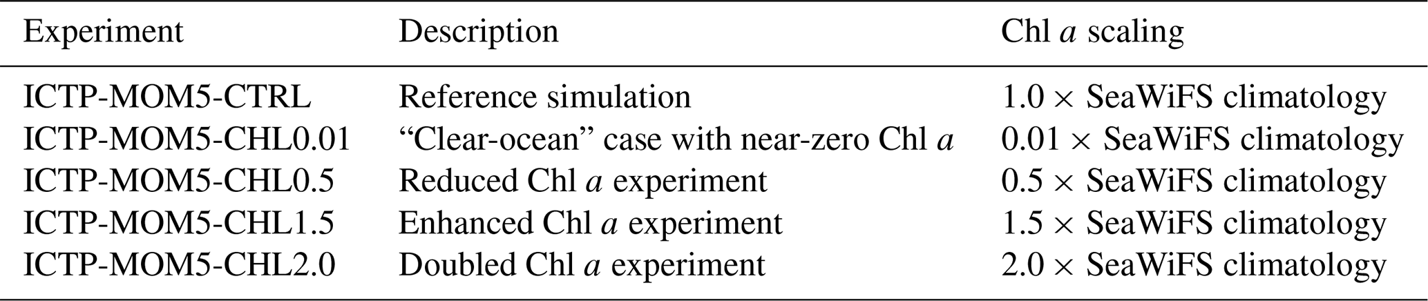
Table 1 Sensitivity experiments performed to assess the bio-physical effect of chlorophyll a concentration (Chl a) on the equatorial Atlantic Ocean mean state and interannual variability. ICTP-MOM5-CTRL serves as the reference simulation (see Sect. 2.2). All sensitivity experiments are identical to the control except for the prescribed monthly Chl a climatology.

In ICTP-MOM5-CTRL, the effect of the presence of phytoplankton on the light absorption is based on Chl a following Manizza et al. (2005). The total surface irradiance, I₀, is split into three wavelength bands: the infrared (I_ir), red visible (I_red), and blue/green visible (I_bg) with a light partitioning of I_ir = 0.58 × I₀, I_red = 0.21 × I₀, and I_bg = 0.21 × I₀, respectively. This leads to a shortwave penetration at depth z (I(z)) of:

$$\begin{array}{}\text{(1)}& I\left(z\right)=I_{\text{ir}}\times e^{-k_{\text{ir}}z}+I_{\text{red}}\times e^{-k_{\text{red}}z}+I_{\text{bg}}\times e^{-k_{\text{bg}}z}\end{array}$$

where k_ir, k_red, and k_bg are light attenuation coefficients. Following Paulson and Simpson (1977), k_ir = 2.86 m⁻¹, whereas k_red and k_bg depend on Chl a as follows (Morel, 1988):

$$\begin{array}{}\text{(2)}& {\displaystyle }& {\displaystyle }{k}_{\text{red}}=\mathrm{0.225}+\mathrm{0.037}\times [\text{Chl }a{]}^{\mathrm{0.629}}\text{(3)}& {\displaystyle }& {\displaystyle }{k}_{\text{bg}}=\mathrm{0.0232}+\mathrm{0.074}\times [\text{Chl }a{]}^{\mathrm{0.674}}\end{array}$$

Hernandez et al. (2017) found only small differences in SST between forced ocean simulations using depth-independent and depth-dependent profiles of Chl a. Therefore, for simplicity and consistency with previous studies, we have used depth-independent profiles of Chl a in all model simulations in this study. However, we note that this represents a limitation because the maximum Chl a concentration is usually found close to the nutricline in the tropical Atlantic Ocean (Herbland, 1983).

To highlight the bio-physical effect on the equatorial Atlantic Ocean mean-state and interannual variability, we performed four sensitivity experiments identical to ICTP-MOM5-CTRL (see Sect. 2.2), except for the prescribed monthly climatology of Chl a (Table 1). In ICTP-MOM5-CHL0.01, the monthly climatology of Chl a is multiplied by 0.01 and aims at simulating a “clear-ocean”, i.e. without Chl a. In ICTP-MOM5-CHL0.5, the monthly climatology of Chl a is reduced by 50 %. In ICTP-MOM5-CHL1.5, it is increased by 50 %, while in ICTP-MOM5-CHL2.0, the monthly climatology is doubled. For clarity, the prescribed monthly climatologies of Chl a averaged over the ATL3 region are shown in Fig. 1b. As defined in Eqs. (2) and (3), the use of these different climatologies of Chl a affects the e-folding depth scale of the light penetration in the visible red ($\mathrm{1}/k_{\text{red}}$) and in the visible blue/green wavelength bands ($\mathrm{1}/k_{\text{bg}}$; Fig. 1c) while the infrared ($\mathrm{1}/k_{\text{ir}}$) is independent. The effect of Chl a is limited for $\mathrm{1}/k_{\text{red}}$, as the e-folding scale is approximately 4 m in all simulations throughout the year (Fig. 1c). In contrast, the effect of Chl a is important for $\mathrm{1}/k_{\text{bg}}$. In ICTP-MOM5-CHL2.0, the ATL3 seasonal cycle of $\mathrm{1}/k_{\text{bg}}$ varies around 14 m, whereas in ICTP-MOM5-CHL0.01 it varies around 40 m. In the following, we examine the biological effect by focusing on the difference between the low Chl a simulation (ICTP-MOM5-CHL0.01) and the control run (ICTP-MOM5-CTRL). Differences between the other runs and ICTP-MOM5-CTRL are documented in the appendix.

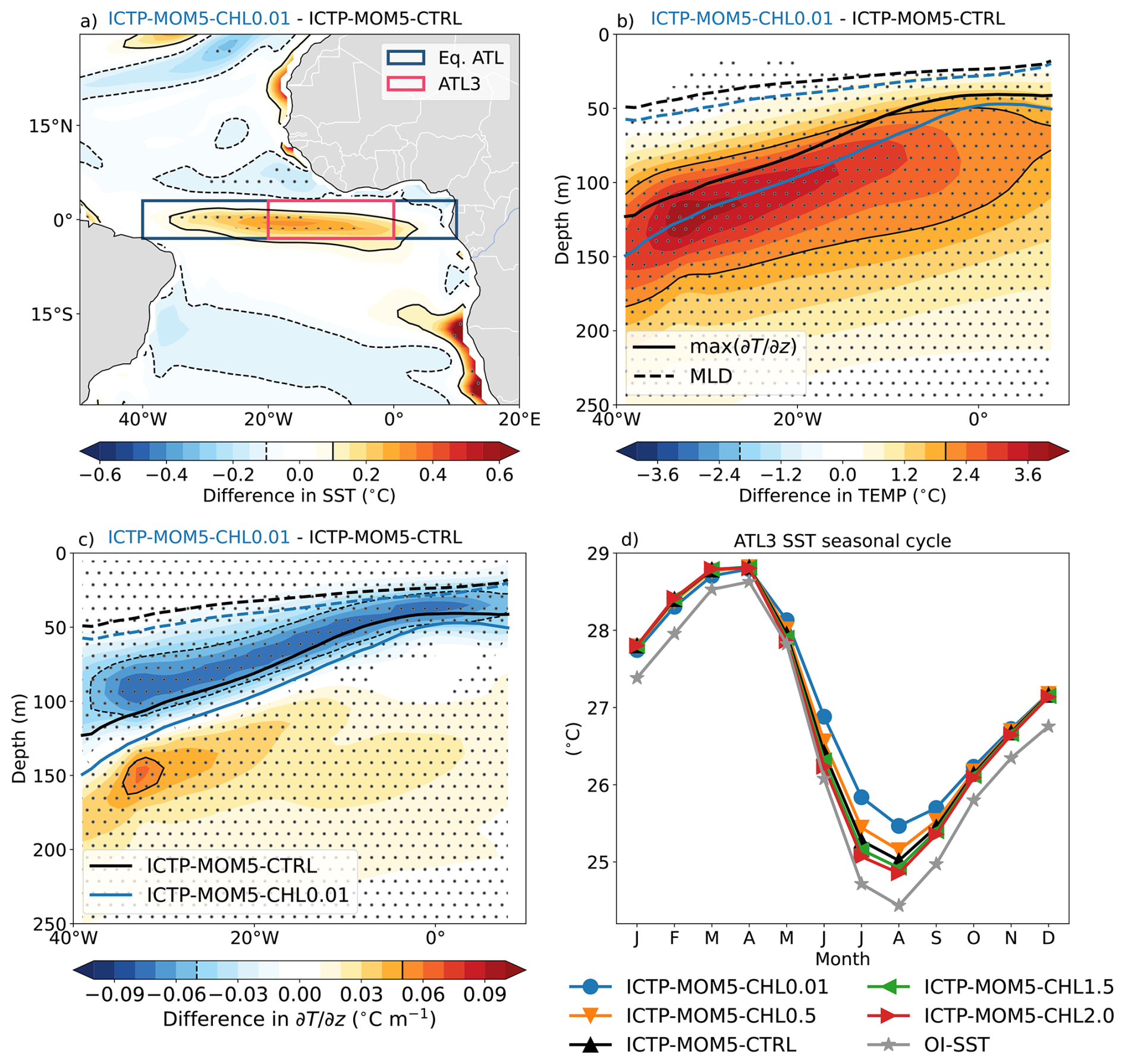
Figure 2 (a) Tropical Atlantic SST difference between ICTP-MOM5-CHL0.01 and ICTP-MOM5-CTRL. Black dashed (solid) contours indicate the −0.1 (0.1) °C difference. The blue and red boxes indicate the equatorial section (3° S–3° N, 40° W–10° E) used in (b, c) and the ATL3 region used in (d). (b) Upper 250 m equatorial Atlantic ocean temperature difference between ICTP-MOM5-CHL0.01 and ICTP-MOM5-CTRL. Black thick dashed and solid lines represent the MLD and $max(\partial T/\partial z)$ from ICTP-MOM5-CTRL, respectively. Similarly, the blue lines are for ICTP-MOM5-CHL0.01. Black dashed (solid) contours indicate the −2 (2) °C difference. (c) Same as (b) but for $\partial T/\partial z$. Black dashed (solid) contours indicate the −0.05 (0.05) °C m⁻¹ difference. Stippling in (a–c) indicate where the difference between the two simulations is statistically significant at the 99 % level according to a bootstrap test (See Sect. 2.3). (d) Seasonal cycle of SST averaged over the ATL3 region for each simulation and OI-SST.

2.3 Analysis methods

To obtain the detrended monthly mean anomalies, the monthly mean model outputs (and observational data, where applicable) are first linearly detrended point-wise over the study period January 1982–December 2020. Then, the monthly climatology of any variable is computed from the detrended data. Finally, the monthly climatology is subtracted to the detrended data to obtain the detrended monthly mean anomalies. Further, a 3-month centered running mean is applied to the detrended anomalies to attenuate the high-frequency variability. In order to preserve the length of the time series, the first and last values of the 3-month centered running mean are based on only two data points. The main regions of interest are the ATL3 region (3° S–3° N, 20° W–0°, red box on Fig. 2a) and the equatorial Atlantic (3° S–3° N, 40° W–10° E, blue box on Fig. 2a) where Atlantic Niños/Niñas occur. The maximum vertical temperature gradient ($max(\partial T/\partial z)$) is used as a proxy for the internal thermocline depth. The mixed-layer depth (MLD) is diagnosed through a density threshold criterion of 0.03 kg m⁻³ increase from the reference value of surface potential density taken at 5 m depth (Griffies, 2012).

To evaluate whether the variability (i.e. standard deviation of anomalies) or the mean state (time mean) differ between two simulations, we apply a nonparametric bootstrap method (Efron and Tibshirani, 1993) independently at each grid point. For the mean-state analysis, the statistic of interest is the difference between the time means of the two simulations, while for the variability analysis it is the difference between their standard deviations. Uncertainty in these differences is estimated using bootstrap resampling with replacement. For each simulation, the time indices are resampled independently 5000 times, and the statistics of interest are computed for each resampled dataset, resulting in a bootstrap distribution of the difference. From this distribution, we estimate a two-sided confidence interval using the 0.5th and 99.5th percentiles. Differences are considered statistically different from zero at the 99 % confidence level when zero falls outside this interval.

3 Results

3.1 Mean-state response

The response of the equatorial Atlantic Ocean mean-state to different monthly climatology of Chl a is investigated by comparing ICTP-MOM5-CTRL against the different sensitivity experiments introduced in Sect. 2.2. Relative to ICTP-MOM5-CTRL, equatorial Atlantic SSTs in ICTP-MOM5-CHL0.01 are significantly warmer between 2° S and 2° N and from 35° W to 2° E (Fig. 2a). In the ATL3 region, the climatological mean SST difference between the two simulations amounts to 0.15 °C. We also note a surface warming along the Angolan and Namibian coasts as well as in the Senegalo–Mauritanian upwelling system (Fig. 2a), which is consistent with results from Hernandez et al. (2017). The ocean temperature differences between these two simulations are not restricted to the surface, as shown by the temperature section difference in the upper 250 m of the equatorial Atlantic (Fig. 2b). Compared to ICTP-MOM5-CTRL, ICTP-MOM5-CHL0.01 reveals a strong and statistically significant warming exceeding 2 °C within 50 m around the mean thermocline depth (Fig. 2b). This subsurface warming in the “clear-ocean” simulation leads to a deepening of the main oceanic thermocline and a weakening of the vertical temperature gradient around the main thermocline (Fig. 2c). A similar response is found when comparing ICTP-MOM5-CHL0.5 to ICTP-MOM5-CTRL (Fig. A1a–c), although with a smaller magnitude (Fig. A1d–f). Conversely, increasing the Chl a by 50 % and 100 % leads to a slight, though not statistically significant, SST cooling (Fig. A1g and j). Furthermore, the equatorial Atlantic Ocean temperature and its vertical gradient in ICTP-MOM5-CHL1.5 and ICTP-MOM5-CHL2.0 only show moderate changes, characterized by subsurface cooling, enhanced vertical temperature gradient around the thermocline, and a slight shoaling of both the thermocline and MLD (Fig. A1g–l).

The eastern equatorial Atlantic SST is characterized by a pronounced seasonal cycle, with maximum values in February–March–April (FMA), when SSTs exceed 28 °C, and minimum values in July–August–September (JAS), when the Atlantic cold tongue develops and SSTs reach 25 °C or lower (Caniaux et al., 2011; Brandt et al., 2023). The amplitude of the seasonal cycle of SST is affected by the changes in vertical distribution of shortwave heating induced by the concentration of Chl a (Fig. 2d). Compared to ICTP-MOM5-CTRL, the amplitude of the ATL3 SST seasonal cycle (defined as the difference between the FMA and JAS seasonal means) is reduced by 14 % in ICTP-MOM5-CHL0.01, from 3.42 to 2.93 °C (Fig. 2d). This reduction mainly results from warmer SSTs in JAS (Fig. 2d), when the Chl a usually peaks in the ATL3 region (Fig. 1b). ICTP-MOM5-CHL0.5 also simulates a reduction where the ATL3 SST seasonal cycle amplitude decreases by 4 % relative to ICTP-MOM5-CTRL. On the contrary, ICTP-MOM5-CHL1.5 and ICTP-MOM5-CHL2.0 show only slight increases in the ATL3 SST seasonal cycle amplitude of 3 % and 1 %, respectively.

Comparing the ATL3 SST seasonal cycle from both control and sensitivity simulations to the one derived from OI-SST shows that ICTP-MOM5 simulations are able to capture the main features of the seasonal cycle of SST in the ATL3 region (Fig. 2d). However, a year-round warm SST bias remains, which is common in ocean and climate models in this region (Richter et al., 2012; Farneti et al., 2022). We note that the idealized increase in Chl a leads to a reduction of the SST bias, particularly in JAS (Fig. 2d). However, this does not necessarily imply that the SST bias in this region results from an incorrect representation of Chl a, but rather highlights the sensitivity of SST to phytoplankton-induced changes in the vertical distribution of shortwave heating.

The surface warming in the equatorial Atlantic in the absence of Chl a is somewhat counterintuitive, as a reduced absorption of the shortwave heat flux near the surface would be expected to lead to local surface cooling, as observed in the open ocean and away from the equator (Fig. 2a). Such a counterintuitive response appears to be related to upwelling regions, as it has already been observed in the equatorial Pacific upwelling (Manizza et al., 2005; Sweeney et al., 2005; Löptien et al., 2009; Park et al., 2014a, b) and in the Senegalo–Mauritanian and Benguela upwelling systems (Frouin et al., 2007; Hernandez et al., 2017). We note that in most previous studies, the bio-physical effect was highlighted by showing the difference between the control run and the experiment (control minus experiment), whereas in this study the difference shown is experiment minus control. The dominant mechanism explaining the surface cooling has been shown to be the vertical redistribution of shortwave heating by Chl a, which enhances upper-ocean stratification and shoals the mixed layer, strengthening total upper-ocean divergent transport by weakening the partially compensating equatorward geostrophic transport. This leads to enhanced equatorial upwelling across the mixed-layer base. Our findings are therefore consistent with this mechanism but exhibit anomalies of the opposite signs.

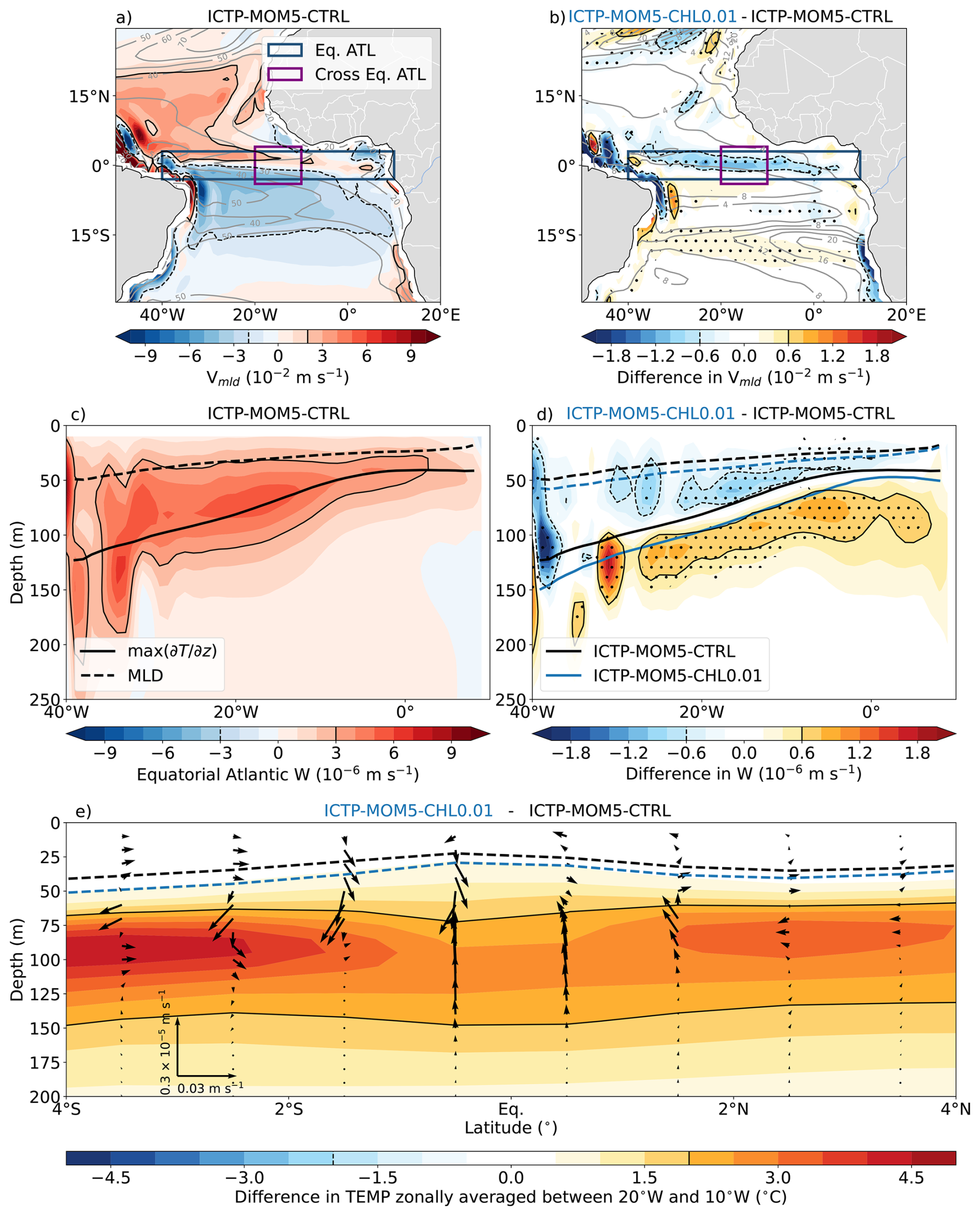
Figure 3 (a) Climatological mixed-layer meridional ocean velocity in ICTP-MOM5-CTRL. Black dashed (solid) contours show −2 (2) × 10⁻² m s⁻¹. Grey contours show mean MLD (20 to 80 m, 10 m interval). (b) Difference in meridional ocean velocity between ICTP-MOM5-CHL0.01 and ICTP-MOM5-CTRL, averaged over their respective MLDs. Black dashed (solid) contours show −0.6 (0.6) × 10⁻² m s⁻¹. Grey contours show MLD differences (−20 to 20 m, 4 m interval) (c) Climatological vertical velocity in the upper 250 m of the equatorial Atlantic (3° S–3° N, 40° W–10° E; blue box in a). Black solid contours denote 3 × 10⁻⁶ m s⁻¹. Black thick dashed and solid lines indicate the MLD and depth of $max(\partial T/\partial z)$, respectively. (d) Same as (c) but for the vertical velocity difference between ICTP-MOM5-CHL0.01 and ICTP-MOM5-CTRL. Black (blue) thick dashed and solid lines indicate the MLD and depth of $max(\partial T/\partial z)$ for ICTP-MOM5-CTRL (ICTP-MOM5-CHL0.01). Stippling in (b, d) indicate where the difference between the two simulations is statistically significant at the 99 % level according to a bootstrap test (See Sect. 2.3). (e) Cross-equatorial Atlantic section (4° S-4° N, zonally averaged between 20 and 10° W; purple box in a) of temperature differences (shading) and meridional and vertical velocity differences (vectors; vertical velocity scaled by 10⁴).

In ICTP-MOM5-CTRL, the meridional ocean velocity averaged over the MLD shows divergence close to the equator driven by trade winds (Fig. 3a), leading to equatorial upwelling (Fig. 3c). In ICTP-MOM5-CHL0.01, this meridional divergence is reduced (Fig. 3b), leading to weaker equatorial upwelling across the base of the mixed layer (Fig. 3d and e). To understand this response we examine the steady zonal momentum budget integrated over the mixed layer, neglecting Reynolds stresses and assuming that baroclinic pressure gradients associated with horizontal density variations are small relative to the barotropic pressure gradient associated with sea surface height variations (Sweeney et al., 2005; Löptien et al., 2009):

$$\begin{array}{}\text{(4)}& M_{\mathrm{y}}=-{\displaystyle \frac{{\mathit{\tau }}_x}{{\mathit{\rho }}_{\mathrm{0}}f}}+{\displaystyle \frac{gD}{f}}{\displaystyle \frac{\partial \mathit{\eta }}{\partial x}}\end{array}$$

where M_y is the meridional transport, D the mixed-layer depth, η the sea surface height, τ_x the zonal wind stress, f the Coriolis parameter, and ρ₀ is a reference density. The meridional transport can be decomposed into a wind-driven Ekman transport (first term on the r.h.s. of Eq. 4) and a compensating geostrophic transport associated with the zonal SSH gradient integrated over the mixed layer (second term on the r.h.s of Eq. 4). Because ICTP-MOM5-CHL0.01 and ICTP-MOM5-CTRL are forced with identical atmospheric forcing (See Sect. 2.2), the reduced poleward transports within the MLD cannot be attributed to changes in Ekman transport. Additionally, the identical trade winds push warm, less dense waters to the west, leading to comparable large-scale zonal SSH gradients in both simulations (not shown). Hence, as zonal SSH gradients remain similar, differences in meridional transports must arise from changes in the MLD.

Under identical wind forcing, a deeper mixed layer can thus strengthen the compensating geostrophic transport, thereby reducing the net meridional transport divergence and weakening equatorial upwelling across the base of the mixed layer. Consistent with this mechanism, ICTP-MOM5-CHL0.01 features deeper MLDs than ICTP-MOM5-CTRL (grey contours in Fig. 3b, dotted line in Fig. 3d, and shadings in Fig. A2a and b). We note that changes in MLD in other simulations are less important Fig. A2c–e. The deepening of the mixed layer is likely due to increased vertical mixing associated with Chl a induced changes in the vertical distribution of shortwave heating. Ultimately, the reduced divergence leads to weaker equatorial upwelling into the mixed layer (Fig. 3d and e) and surface warming in the “clear-ocean” simulation (Fig. 2a).

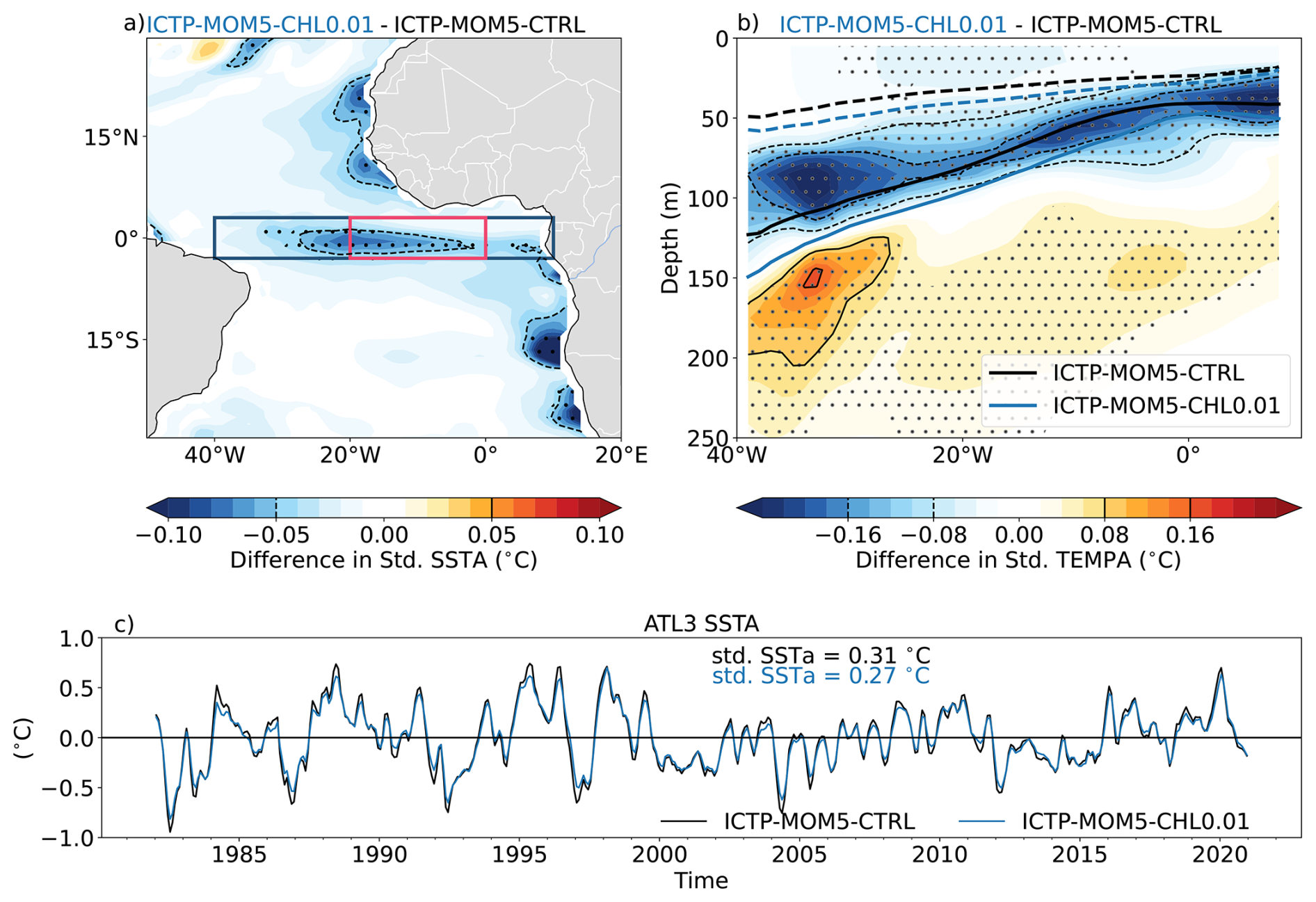
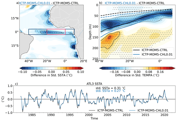
Figure 4 (a) Difference in the standard deviation of detrended SST anomalies between ICTP-MOM5-CHL0.01 and ICTP-MOM5-CTRL. Black dashed (solid) contours indicate −0.05 °C (0.05 °C). The blue and red boxes denote the equatorial Atlantic (Eq. ATL; 3° S–3° N, 40° W–10° E) and the ATL3 region (3° S–3° N, 20° W–0° E) regions, respectively. (b) Difference in the standard deviation of the upper 250 m of the equatorial Atlantic TEMP anomalies between ICTP-MOM5-CHL0.01 and ICTP-MOM5-CTRL. Black dashed (solid) contours indicate −0.16 and −0.08 °C (0.08 and 0.16 °C). Black stipplings in (a) and (b) indicate regions where the difference in standard deviation is statistically significant at the 99 % level according to a bootstrap test (see Sect. 2.3). (c) Time series of detrended ATL3-averaged SST anomalies for ICTP-MOM5-CTRL (black) and ICTP-MOM5-CHL0.01 (blue).

Although outside the scope of this paper, we note that Chl a seems to exert a non-trivial effect on the vertical structure of the tropical cell. Indeed, the maximum vertical velocity (around 100 m at 20° W; Fig. 3c) occurs at the interface of the upper and lower branches of the tropical cell (Stommel, 1960; McCreary, 1981; Webb, 2018). Above this level, the poleward Ekman velocity is greater than the zonal pressure gradient, giving rise to a net poleward velocity (as previously discussed). The depth of the upper branch of the tropical cell seems to be related to the depth at which irradiance drops to 1 % of its surface value (around 100–150 m), often used to define the base of the euphotic zone. Below this interface, the zonal pressure term dominates, resulting in an equatorward velocity and closing the cell. The upward shift of the maximum vertical velocity (Fig. 3d) suggests that Chl a reduces the depth of the interface between the upper and lower parts of the tropical cell, increasing poleward velocities above the interface and reducing equatorward velocities below. In fact, the depth of the maximum vertical velocity in the ATL3 region is 10 m shallower in ICTP-MOM5-CTRL (54 m) than in ICTP-MOM5-CHL0.01 (64 m). In addition, the magnitude of the maximum vertical velocity is reduced by 6.4 % in ICTP-MOM5-CHL0.01 (4.4 × 10⁻⁶ m s⁻¹) relative to ICTP-MOM5-CTRL (4.7 × 10⁻⁶ m s⁻¹). We also observe that Chl a strengthens and shoals the core of the equatorial undercurrent (Fig. A3). An in-depth analysis of whether velocities are modified by the altered vertical extent of each branch or partly due to a change in the total transport is left for a future study.

3.2 Interannual variability response

In addition to modifying the ocean mean-state, the presence of Chl a can also affect interannual SST variability. Park et al. (2014a, b) showed that, in the equatorial Pacific Ocean, forced ocean model simulations without, or with reduced, Chl a simulated weaker interannual SST variability than simulations with realistic Chl a levels. In the following, we assess the effect of different levels of Chl a on the equatorial Atlantic interannual SST variability (Figs. 4 and A4).

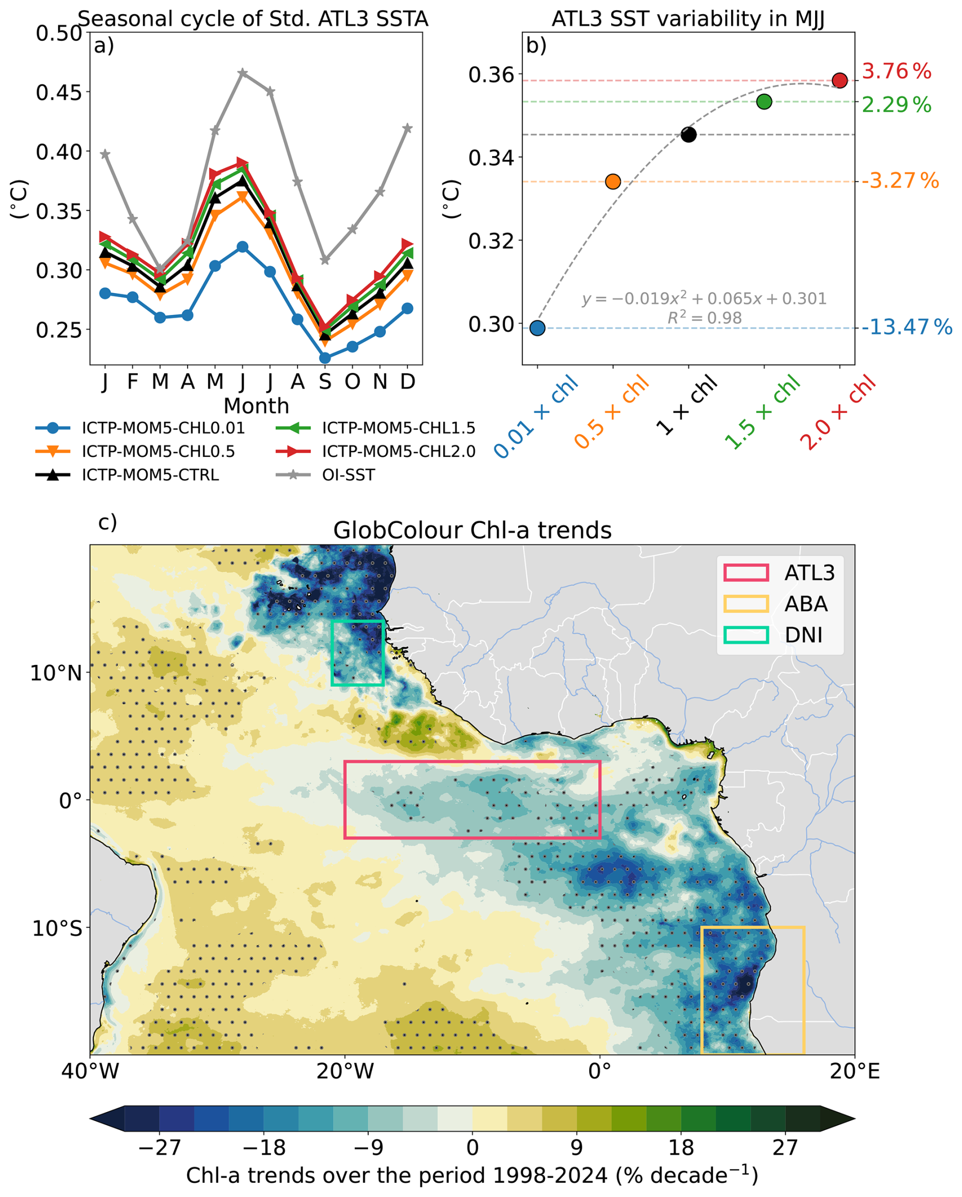
Figure 5 (a) Seasonal cycle of the standard deviation of the detrended SST anomalies averaged over the ATL3 region for ICTP-MOM5-CHL0.01 (blue), ICTP-MOM5-CHL0.5 (orange), ICTP-MOM5-CTRL (black), ICTP-MOM5-CHL1.5 (green) and ICTP-MOM5-CHL2.0 (red). The red, orange, and green boxes in (c) indicate the ATL3, ABA (20–10° S, 8–16° E), and DNI (9–14° N, 21–17° W) regions, respectively. (b) Scatter diagrams showing the standard deviation of SST anomalies averaged over the ATL3 region in function of the prescribed Chl a seasonal cycle as indicated on the x-axes. The right y-axis shows the percentage of change in SST variability relative to the ICTP-MOM5-CTRL value. (c) Linear trends in Chl a over January 1998–December 2024. Trends are computed from a linear least-squares fit applied to monthly mean Chl a time series at each grid point. The resulting slope ($\mathrm{mg}{\mathrm{m}}^{-\mathrm{3}}{\mathrm{month}}^{-\mathrm{1}}$) is converted to $\mathrm{mg}{\mathrm{m}}^{-\mathrm{3}}{\mathrm{decade}}^{-\mathrm{1}}$ by multiplying by 120 (12 months × 10 years). Relative trends are then expressed in % decade⁻¹ by dividing by the climatological mean chlorophyll concentration at each grid point and multiplying by 100. Grey stipplings indicate regions showing a statistically significant trend at the 95 % level according to a Student's t-test.

ICTP-MOM5-CHL0.01 shows a statistically significant reduction in interannual SST variability in the central equatorial Atlantic, particularly between 30° W and 0° E (Fig. 4a). ICTP-MOM5-CHL0.5 (ICTP-MOM5-CHL1.5 and ICTP-MOM5-CHL2.0) also exhibits reduced (enhanced) interannual SST variability in the central equatorial Atlantic. However, these changes are not significant at the 99 % level (Fig. A4).

The reduction in SST variability is also evident in the time series of the ATL3-averaged SST anomalies (Fig. 4c), with standard deviations of 0.31 °C for ICTP-MOM5-CTRL and of 0.27 °C for ICTP-MOM5-CHL0.01, corresponding to a 12.9 % reduction. We note that the interannual ATL3 SST variability in ICTP-MOM5-CTRL is underestimated compared to that of OI-SST, which has a standard deviation of the ATL3 SST anomalies of 0.38 °C over the period 1982–2020. This underestimation in the ocean model is likely due to the atmospheric forcing (JRA55-do), as shown by Prigent and Farneti (2024).

The effect of Chl a on the interannual temperature variability is not restricted to the surface. The ocean temperature variability in the upper 150 m of the equatorial Atlantic (3° S–3° N, 40° W–10° E) is also significantly reduced in ICTP-MOM5-CHL0.01 (Fig. 4b). As all simulations are forced with identical winds, thermocline depth variations are similar across simulations (Fig. A5) and therefore cannot explain the changes in temperature variability. Instead, the reduced subsurface temperature variability in the vicinity of the thermocline is explained by the weakened vertical temperature gradient around the thermocline in ICTP-MOM5-CHL0.01 (Fig. 2c). Additionally, weakened equatorial upwelling across the basis of the mixed layer (Fig. 3d) also contributes to the reduced interannual SST variability in ICTP-MOM5-CHL0.01. Similar but weaker reductions are found when comparing ICTP-MOM5-CHL0.5 to ICTP-MOM5-CTRL (Fig. A4c and d). In contrast, and although these changes are not statistically significant, both ICTP-MOM5-CHL1.5 and ICTP-MOM5-CHL2.0 exhibit increased subsurface temperature variability in the equatorial Atlantic (Fig. A4e–h), consistent with the enhanced vertical temperature gradient in those simulations (Fig. A1i and l).

Next, we examine the response of the interannual ATL3 SST variability to varied levels of Chl a. The response is strongest in May–June–July and November–December, which correspond to the peak seasons for the Atlantic Niño and Atlantic Niño II (Fig. 5a), respectively. The seasonal cycle of the ATL3 SST variability is well captured by ICTP-MOM5-CTRL, although with too weak variability throughout the year (Fig. 5a). The response of the interannual ATL3 SST variability in May–June–July to prescribed Chl a is non-linear, with a quadratic fit explaining 98 % of the variance (Fig. 5b). The ATL3 interannual SST variability in May–June–July is of 0.345 °C in ICTP-MOM5-CTRL. Relative to this value, ICTP-MOM5-CHL1.5 and ICTP-MOM5-CHL2.0 show small increases of 2.29 % and 3.76 %, respectively, while ICTP-MOM5-CHL0.5 and ICTP-MOM5-CHL0.01 depict decreases of 3.27 % and 13.47 %, respectively.

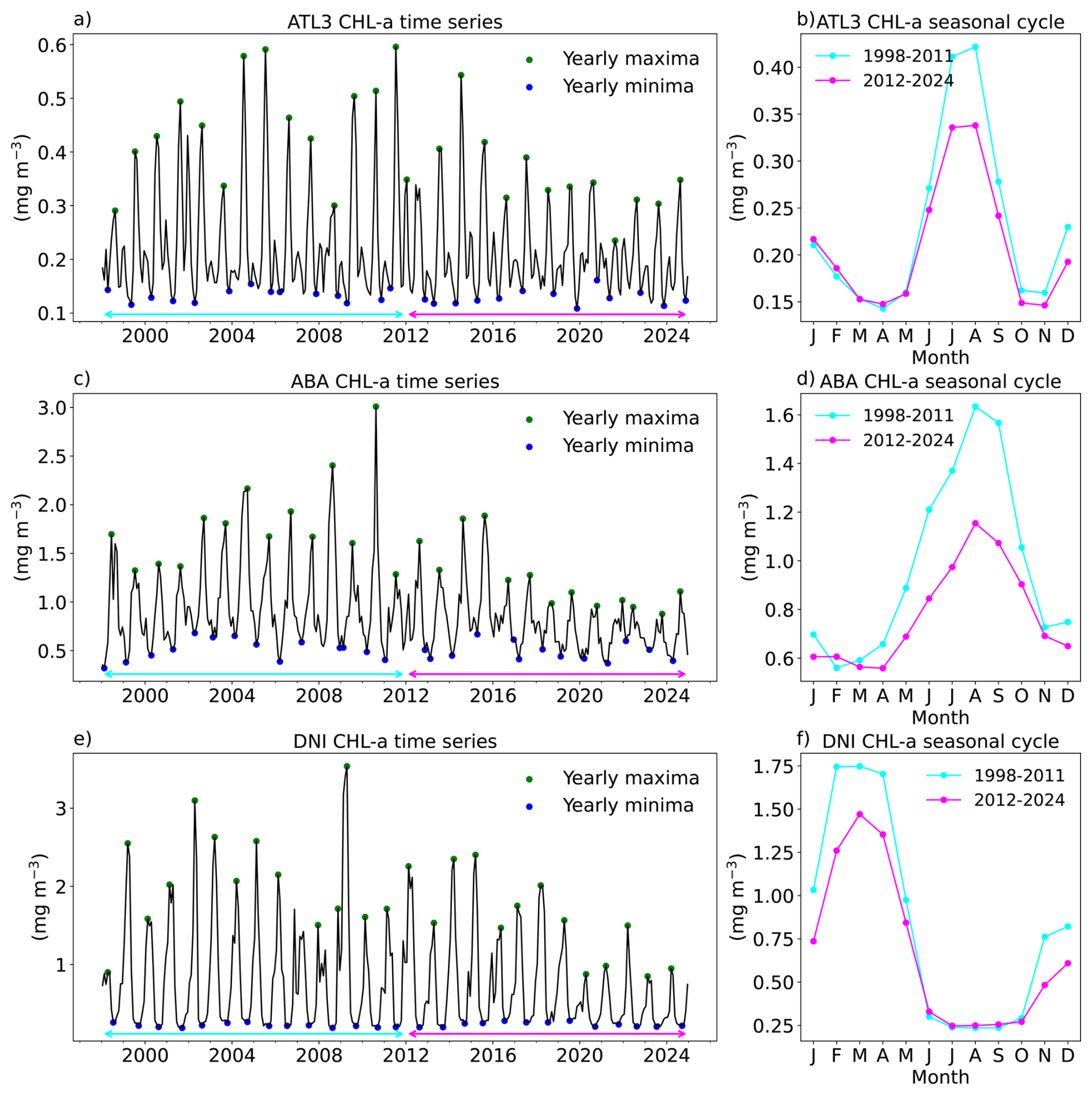
Figure 6 (a) Time series of Chl a from the GlobColour satellite ocean colour product, averaged over the ATL3 region, for the period from January 1998 to December 2024. Green (blue) dots indicate the yearly maxima (minima). The cyan (magenta) arrow denotes the period from January 1998–December 2011 (January 2012–December 2024). (b) Seasonal cycle of the ATL3 Chl a from GlobColour evaluated over 1998–2011 (cyan) and 2012–2024 (magenta). (c, d) Same as (a, b) but for the ABA (orange box in Fig. 5c; 20–10° S, 8–16° E) region. (e, f) Same as (a, b) but for the DNI (green box in Fig. 5c; 9–14° N, 21–17° W) region.

The fact that changes in the mean state of Chl a affect the interannual SST variability in the tropical Atlantic Ocean is of particular interest, as a merged satellite product of Chl a (GlobColour) shows marked trends over the period 1998–2024 (Fig. 5c). Similar trends have also been reported in recent studies (Zhao et al., 2025; Hong et al., 2025; Silsbe et al., 2025). The timeseries of the GlobColour Chl a averaged over the ATL3 region reveals a clear reduction in the yearly maxima, while the yearly minima remain stable (Fig. 6a). Comparing the seasonal cycle of the merged satellite product of Chl a averaged over the ATL3 region during 1998–2011 with the one obtained over 2012–2024 reveals that the largest decrease occurs during July-August-September, the season of maximum Chl a (Fig. 6b). These ongoing changes in Chl a in the tropical Atlantic Ocean underscore the need to improve our understanding of the relationship between Chl a and interannual SST variability in the tropical Atlantic.

4 Discussion and Conclusions

We investigated the equatorial Atlantic Ocean mean-state and interannual variability responses to modified shortwave heating distributions induced by Chl a using an ocean model and by carrying out a suite of sensitivity experiments. Our results showed significant responses when comparing a “clear-ocean” simulation, including a satellite-based climatology of Chl a multiplied by 0.01 (ICTP-MOM5-CHL0.01), to a “realistic” simulation, using the original Chl a climatology (ICTP-MOM5-CTRL).

Compared with ICTP-MOM5-CTRL, ICTP-MOM5-CHL0.01 simulates an equatorial Atlantic mean-state characterized by:

• A 0.15 °C warming and a 14 % reduction of the amplitude of the SST seasonal cycle in the ATL3 region (Fig. 2).

• A subsurface warming, along with a reduced vertical temperature gradient around the thermocline and deepened thermocline (Fig. 2).

• A deepened MLD slightly off the equatorial region, which strengthens the mixed-layer-integrated geostrophic transport associated with the zonal SSH gradient, thereby reducing the net meridional transport divergence and weakening equatorial upwelling into the mixed layer, consistent with previous studies in the equatorial Pacific (Sweeney et al., 2005; Löptien et al., 2009; Park et al., 2014a, b).

The response of interannual SST and subsurface temperature variability in the equatorial Atlantic Ocean to Chl a-induced shortwave heating redistribution is assessed by comparing ICTP-MOM5-CHL0.01 with ICTP-MOM5-CTRL, revealing:

• A reduction of 12.9 % of the ATL3 SST variability from 0.31 to 0.27 °C (Fig. 4a and c).

• A reduction of the equatorial Atlantic subsurface temperature variability (Fig. 4b), which is linked to changes in the vertical temperature gradient and equatorial upwelling.

• The reduction of the ATL3 SST variability is most pronounced in May–June–July, with a reduction of 13.47 % from 0.345 to 0.298 °C (Fig. 5a)

Furthermore, the analysis of additional simulations showed that the interannual SST variability in the equatorial Atlantic upwelling system responds non-linearly to different levels of Chl a (Fig. 5b). By analyzing a merged satellite product of Chl a we found that, over the period from 1998 to 2024, the Chl a seems to decline in the eastern equatorial Atlantic (Fig. 5c). We acknowledge that this decline in Chl a has already been reported in recent studies (Zhao et al., 2025; Hong et al., 2025; Silsbe et al., 2025). Our results thus suggest that this decline could have contributed to the weakened interannual SST variability observed after 2000 in the ATL3 region (Prigent et al., 2020). We also note that the Chl a is declining in the tropical Angolan and Senegalo–Mauritanian upwelling systems (Figs. 5c and 6). These two coastal regions exhibit large interannual SST variability driven by extreme warm and cold coastal events, called Benguela Niños/Niñas for the tropical Angolan upwelling system (Shannon et al., 1986) and Dakar Niños/Niñas for the Senegalo–Mauritanian upwelling system (Oettli et al., 2016). Therefore, the link between interannual SST variability and Chl a in those regions should be examined in further studies.

Since our model simulations were not coupled to a biogeochemical model, we could not investigate the potential impact of interannual variations in Chl a concentration on interannual SST variability in the tropical Atlantic Ocean. Park et al. (2014a) showed that interannually varying Chl a can have a damping effect on ENSO. In other words, during a La Niña event, trade winds are enhanced, leading to increased upwelling and supply of nutrients, which result in anomalously high Chl a concentration that traps more solar radiation in the upper layer, thereby damping the negative SST anomaly. The opposite effect occurs during an El Niño event due to the reduction in nutrients supply. Such a damping effect is also likely active in the tropical Atlantic, as interannual variations in SST and Chl a (or net primary production) have been found to occur concomitantly in the equatorial Atlantic (Grodsky et al., 2008; Chenillat et al., 2021), as well as in the tropical Angolan (Imbol Koungue et al., 2024) and Senegalo–Mauritanian (Imbol Koungue et al., 2025) upwelling systems. Therefore, further studies using coupled ocean-atmosphere-biogeochemical simulations are needed to investigate this damping effect in the tropical Atlantic Ocean.

Appendix A: Climatological Mean State and Interannual Variability responses to Chlorophyll a Concentration in ICTP-MOM5 Sensitivity Experiments

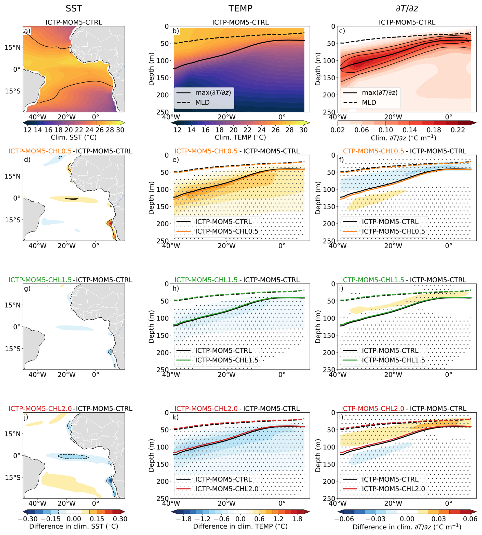
Figure A1 Climatological mean (a) SST, (b) temperature in the upper 250 m of the equatorial Atlantic (3° S–3° N, 40° W–10° E), and (c) vertical temperature gradient in the upper 250 m of the equatorial Atlantic from ICTP-MOM5-CTRL over the period 1982–2020. In (b, c) the black thick dashed (continuous) line indicates the MLD ($max(\partial T/\partial z)$). Difference between ICTP-MOM5-CHL0.5 and ICTP-MOM5-CTRL in terms of (d) SST, (e) temperature, and (f) vertical temperature gradient. (g–i) Same as (d–f) but between ICTP-MOM5-CHL1.5 and ICTP-MOM5-CTRL. (j–l) Same as (d–f) but between ICTP-MOM5-CHL2.0 and ICTP-MOM5-CTRL. Stipplings indicate regions where the difference in mean-state is significantly different according to a bootstrap test (see Sect. 2.3). We note that the range of the colorbars differ from Fig. 2.

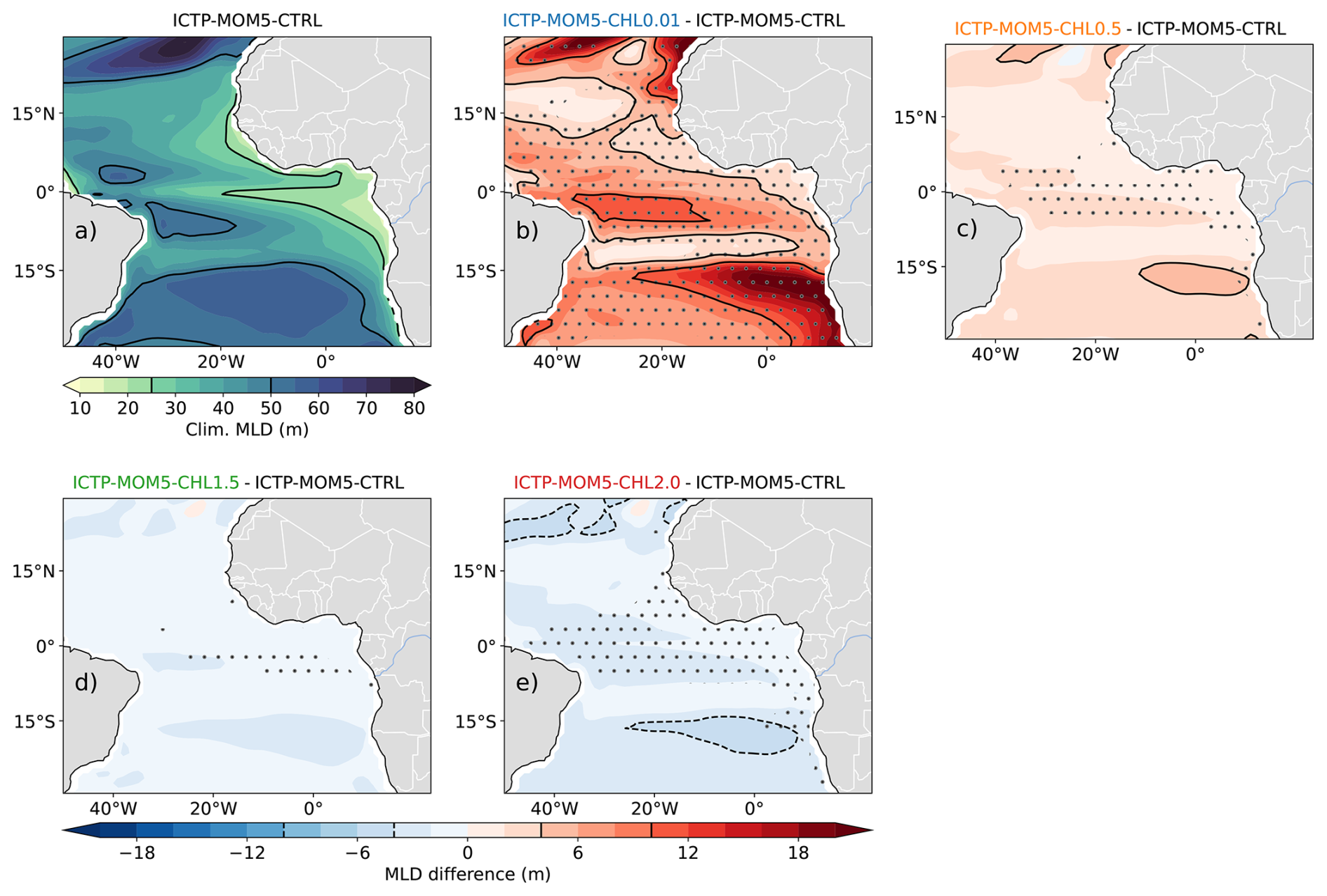
Figure A2 (a) Climatological mean tropical Atlantic mixed layer depth for ICTP-MOM5-CTRL. Black contours indicate the 25 and 50 m MLDs. Difference in climatological mean MLD between between ICTP-MOM5-CTRL and (b) ICTP-MOM5-CHL0.01, (c) ICTP-MOM5-CHL0.5, (d) ICTP-MOM5-CHL1.5, and (e) ICTP-MOM5-CHL2.0. Dashed (solid) black contours indicate the −10 and −4 m (4 and 10 m) differences.

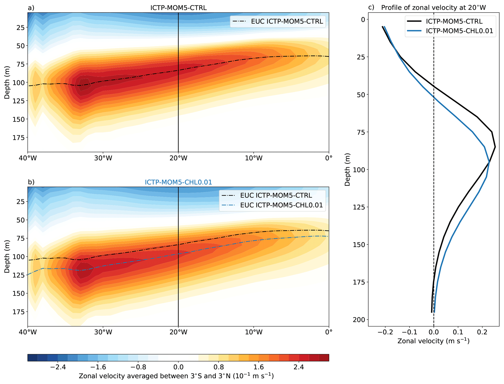
Figure A3 (a) Equatorial section (3° S–3° N, 40° W–0° E) of zonal velocity for (a) ICTP-MOM5-CTRL and (b) ICTP-MOM5-CHL0.01. The dashed-dotted lines indicate the depth of the core of the Equatorial Undercurrent (EUC). The EUC core depth is defined as the depth of the maximum eastward zonal velocity. For each vertical profile, the maximum velocity is first identified, and a quadratic interpolation through the maximum and its two neighboring depth levels is then used to estimate the peak depth continuously. If the maximum occurs at a profile boundary, the corresponding model depth is retained. (c) Vertical profile of zonal velocity at 20° W, averaged between 3° S–3° N, for ICTP-MOM5-CTRL (black) and ICTP-MOM5-CHL0.01 (blue).

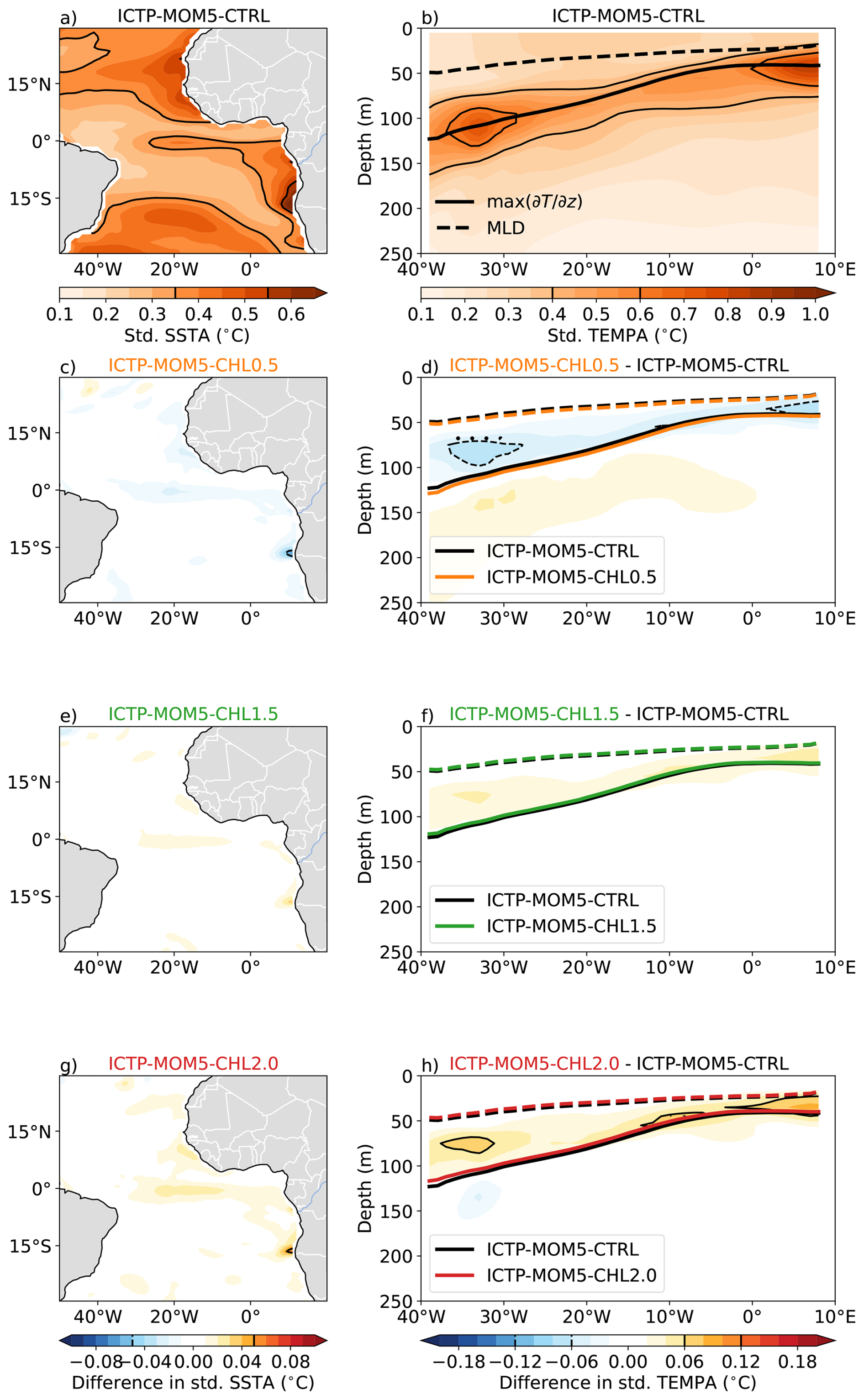
Figure A4 Standard deviation of (a) detrended SST anomalies, (b) temperature anomalies in the upper 250 m of the equatorial Atlantic (3° S–3° N, 40° W–10° E) from ICTP-MOM5-CTRL over the period 1982–2020. In (b) the black thick dashed (continuous) line indicates the MLD ($max(\partial T/\partial z)$). Difference between ICTP-MOM5-CHL0.5 and ICTP-MOM5-CTRL in terms of (c) SST and (d) temperature variability. In (c) black dashed (solid) contours indicate −0.05 °C (0.05 °C). In (d) black dashed (solid) contours indicate −0.12 and −0.06 °C (0.06 and 0.12 °C). (e, f) Same as (c, d) but between ICTP-MOM5-CHL1.5 and ICTP-MOM5-CTRL. (g, h) Same as (c, d) but between ICTP-MOM5-CHL2.0 and ICTP-MOM5-CTRL. Stipplings indicate regions where the difference in mean-state is significantly different according to a bootstrap test (see Sect. 2.3). We note that the range of the colorbars differ from Fig. 4.

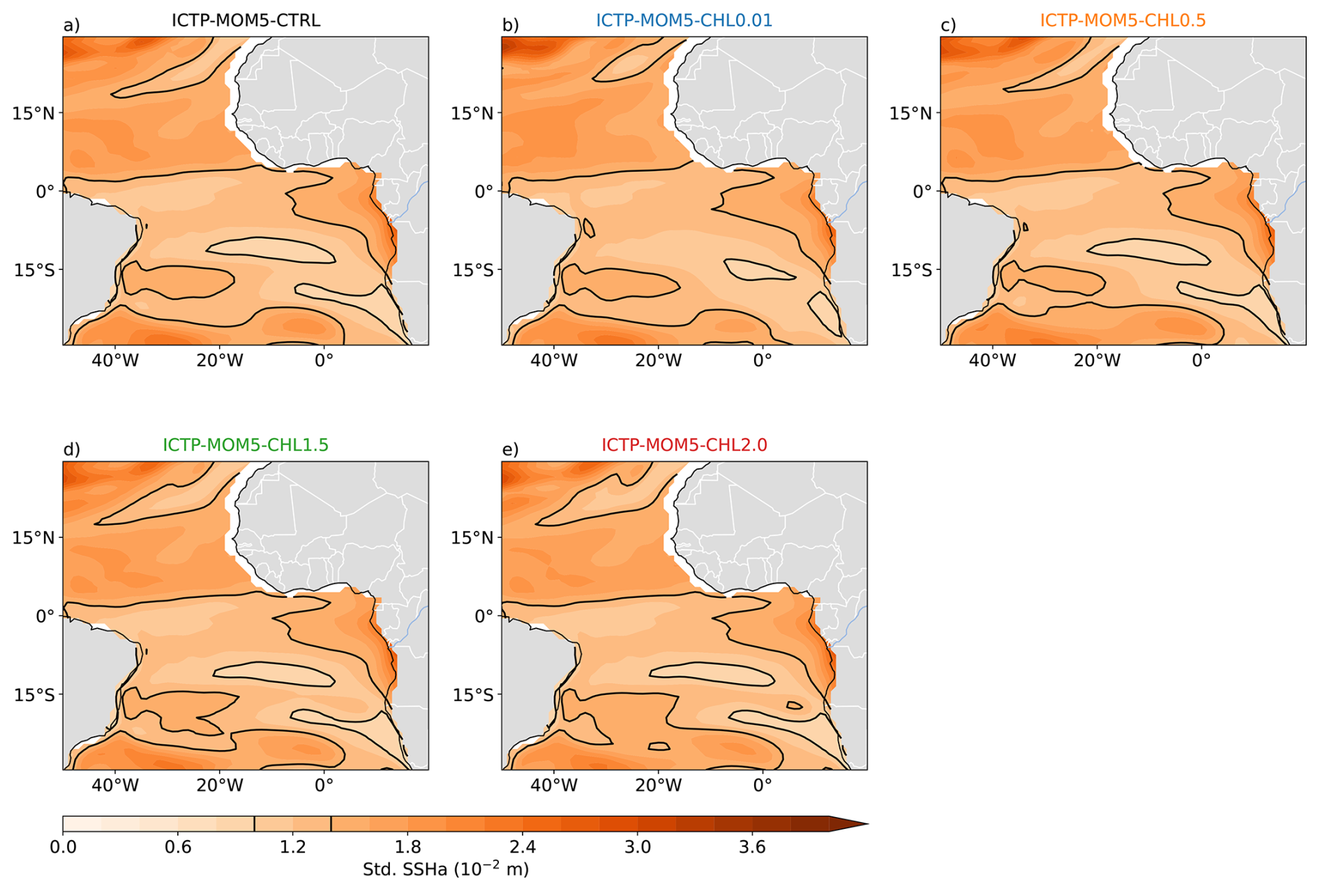
Figure A5 Standard deviation of detrended SSHA over the period 1982–2020 for (a) ICTP-MOM5-CTRL, (b) ICTP-MOM5-CHL0.01, (c) ICTP-MOM5-CHL0.5, (d) ICTP-MOM5-CHL1.5, and (e) ICTP-MOM5-CHL2.0. Black contours denote the 0.01 and 0.014 m standard deviation levels.