Bottom mixed layer derivation and spatial variability over the central and eastern abyssal Pacific Ocean

The bottom mixed layer (BML) of the abyssal ocean regulates heat exchange between the deep interior and seafloor, driving water–mass transformation and influencing global circulation. Spatial variability of the BML was examined in the under-sampled abyssal Pacific Ocean using surface-to-seafloor temperature and pressure observations over 4 months in 2023–2024. Given the typical decadal repeat rate of global hydrographic sections, subdecadal variability in the abyssal ocean has remained poorly resolved. Our observations contribute towards filling this gap for the central and eastern abyssal Pacific Ocean. Four methods were used to determine the BML thickness, with the threshold method providing the most reliable estimates. The mean BML thickness was (226 ± 172 m) with added repeat hydrographic sections providing context and additional data points. At each BML data point we determined the slope, the terrain roughness and the extracted predicted internal tide energy dissipation (over five different low-mode processes and high-mode local processes) at 50 km scales from publicly available datasets. These factors were input into a Random Forest Regressor (RF) model, the first time machine learning techniques have been applied to investigate BML thickness. The RF feature importance scores identified bottom depth, total internal tide energy dissipation, followed by slope, as the strongest predictors of BML thickness, revealing the importance of low-mode internal wave energy losses in this abyssal setting. Targeted and sustained observations near the seafloor at gateway regions of abyssal pathways are vital for understanding energy exchange that influences meridional overturning circulation. Our results highlight a regime where sustained low-mode internal tide energy loss, modulated by topographic slope and depth, governs the BML thickness in the abyssal Pacific. However, the rate at which BML thickness changes over time and the processes that cause these changes remain key unresolved factors.

1 Introduction

Nearly half the Pacific Ocean comprises abyssal zones that have experienced persistent warming in the past 30 years (Johnson and Purkey, 2024). The bottom mixed layer (BML), a well-mixed region directly above the seafloor in the abyssal ocean (Armi and Millard, 1976; Lentz and Trowbridge, 1991) is a critical interface where turbulent mixing facilitates exchange between the deep ocean interior and the seafloor, influencing water–mass transformation and global circulation. Dynamics within the BML are affected by internal wave activity (Zulberti et al., 2022; Holmes et al., 2016), and near-boundary turbulence (Lentz and Trowbridge, 1991; van Haren et al., 2024), impacting diapycnal mixing, deep-sea food web connectivity, and heat transport (Jayne et al., 2004). Additionally, the BML region may contribute to abyssal mixing, as the interplay of turbulent processes through internal tides and stratification here facilitates diapycnal mixing (Kunze et al., 2012), thereby helping to drive the meridional overturning circulation (MOC) (Wunsch and Ferrari, 2004; de Lavergne et al., 2017; Ferrari et al., 2016). MOC is sustained by the abyssal flow of North Atlantic Deep Water (NADW) and Antarctic Bottom Water (AABW), which transport dense water masses equatorward and poleward from their formation regions through the deep ocean. The pathways involved in the MOC have been broadly identified, with general consensus on their origins, particularly in the ventilation regions adjacent to Antarctica (AABW) and the Labrador Sea (NADW) (Ferrari et al., 2016; Talley, 2013). While the broad pathways of these abyssal waters are accepted, the detailed mechanisms by which they return to the surface through diapycnal mixing and upwelling remain active areas of research (Marshall and Speer, 2012; van Haren et al., 2024; Wynne-Cattanach et al., 2024; de Lavergne et al., 2017; Drake et al., 2022). Regions of intense abyssal mixing over mid-ocean ridges and narrow inter-basin channels are key sites where stratification governs regional variability in the BML, current pathways and internal tide generation, connecting closely to abyssal pathways, while seafloor topography remains the primary control on BML thickness at the global scale (Gula et al., 2016). However, the relative importance between topography, its spatial scales, and the dynamic processes within ocean basins dictating the BML thickness remains unclear (Weatherly and Martin, 1978; de Lavergne et al., 2017).

The strength of deep MOC in the Pacific Ocean has been historically underestimated due to a lack of data and its complex topographies, making simulations more challenging (Kawabe and Fujio, 2010; Oka and Niwa, 2013). Broadly, AABW enters the Pacific Ocean along the eastern side of the Tonga–Kermadec Ridge (Chandler et al., 2024), then narrows through the Samoan Passage (Alford et al., 2013) before bifurcating to the west and north towards the Japan Trench (Kawabe and Fujio, 2010) (Fig. 1). North of the Samoan Passage, there is also bottom water transport to the east and south of the Hawaiian Ridge. Around the Hawaiian Ridge, energetic baroclinic tides are generated over the rough seafloor, contributing to distinct differences in the eastern and western regions of the Pacific Ocean, with larger dissipation in the western Pacific (Hautala, 2018; Alford et al., 2007). AABW transforms into North Pacific Deep Water (NPDW) while reaching the North Pacific. It is then further transformed through deep ocean mixing while traveling south and reinforcing subsurface stratification and linking to deep convection in the Southern Ocean (Tatebe et al., 2018).

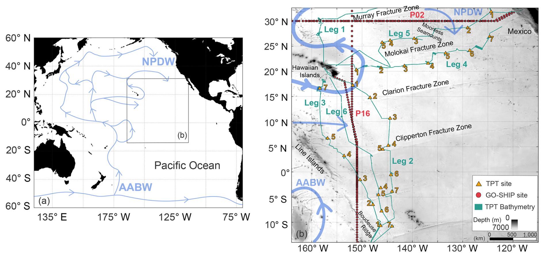
Figure 1 (a) Bottom water circulation pathways through the Pacific Ocean based on existing research (Kawabe and Fujio, 2010; Oka and Niwa, 2013; Hautala, 2018) with (b) insert as the extent of the study region. AABW = Antarctic Bottom Water, NPDW = North Pacific Deep Water (b) Study region boundary, locations, and features, including a regional bathymetric grid. Orange triangles are the Trans-Pacific Transit Expedition deployment locations, with numbers as the site number within the associated leg. The R/V Dagon multibeam echosounder coverage is displayed in green. Note that Leg 1 is not used in this analysis. The GO-SHIP repeat hydrographic lines and deployment locations are marked with red circles (P16 and P02). Blue arrows are bottom water circulation pathways adapted from previous studies. Background regional bathymetry is from the Global Multi-Resolution Topography (GMRT) Synthesis (Ryan et al., 2009). Released CC BY 4.0 Deep | Attribution 4.0 International | Creative Commons.

While rough and variable topography can modulate the BML thickness (e.g. fracture zones (Thurnherr et al., 2020) and seamounts (Mashayek et al., 2024)) regions of the seafloor with broadly similar depths or geomorphology can nevertheless exhibit vastly different BML thicknesses due to differences in ocean dynamics such as boundary currents or abyssal transformations (Drake et al., 2022; Holmes et al., 2018). Along continental shelf regions, it is on the order of 40–70 m in the South China Sea (Liu et al., 2023) and 5–15 m along the Northern California Shelf (Lentz and Trowbridge, 1991). The mean BML thickness over different latitudes in the North Atlantic Basin has been reported as 30–60 m (Lozovatsky and Shapovalov, 2012). Across the Drake Passage, it was found to be over 100 m, similar to Gulf Stream regions (Todd, 2017). These differences may also be due to methodology. For example, the region immediately north of the Puerto Rico Trench in the North Atlantic (21° N, 66° W) has a BML thickness reportedly ranging from 80–800 m (Fig. 9 in Banyte et al., 2018), 60–100 m (Fig. 2b in Lozovatsky and Shapovalov, 2012) and 80 m (Fig. 1 in Huang et al., 2019) with the variation likely attributed to different methodology and spatial interpolation.

The transfer of mass and momentum between the ocean interior and the seafloor occurs via the BML. Yet in most large-scale ocean circulation models, it is generally unrepresented. As a result, robust parameterizations of bottom boundary processes are essential (Legg et al., 2006; Fox-Kemper et al., 2019). Munk (1966) initially proposed a vertically integrated, one-dimensional framework to estimate diapycnal mixing rates averaged across the ocean interior. However, it has been subsequently found that mixing in the bottom boundary is inherently three-dimensional, shaped by turbulent processes influenced by topography and internal wave dynamics (Kunze et al., 2012; Polzin et al., 2014; Wunsch, 2023). Simple bottom boundary layer parameterizations assume local, steady-state velocity shear and stratification relationships to simulate turbulent mixing and momentum transfer vertically, potentially neglecting variability in the BML thickness (Large et al., 1994). Recent improvements have incorporated wave-driven turbulence and terrain-following schemes (Arbic et al., 2009), some of which include profiles of diffusivity and viscosity in their parameterization (Fox-Kemper et al., 2019). Nevertheless, additional observations along the ocean's bottom boundary remain crucial, not only for validating models, but for resolving the spatial and temporal variability in the BML structure that underpins interior-seafloor exchange (de Lavergne et al., 2017; Ferrari et al., 2016; van Haren et al., 2024; Wynne-Cattanach et al., 2024).

The BML thickness is most commonly defined as the thickness above the seabed at which a variable (typically conservative temperature or density) deviates from the seafloor value by a specified threshold (also known as the “threshold method”). While we use a hydrographic definition of the mixed layer, it is important to note that this does not necessarily coincide with the dynamically active mixing layer defined by turbulence; distinguishing these layers is increasingly recognized as essential when inferring mixing intensity and water–mass transformation. While we refer to this as the bottom mixed layer, its thickness may reflect varied bottom boundary processes, not exclusively active mixing. It is inhomogeneous throughout the world's oceans, not only because of the varying depth and roughness of the seafloor but also because of the influence of differing oceanographic processes in each region. Different oceanographic conditions require varying thresholds to calculate the BML thickness. For instance, weakly stratified abyssal regions necessitate small density thresholds ($\mathrm{1}\times {\mathrm{10}}^{-\mathrm{3}}$ kg m⁻³), while highly turbulent areas are better suited to larger threshold values (Fig. 1 in Banyte et al., 2018), or sensitivity in the threshold value may be directly related to instrument noise (Lentz and Trowbridge, 1991). To overcome sensitivity and subjectivity in threshold (or gradient) selections, approaches like the relative variance (Huang et al., 2018b) and integrated methods (Huang et al., 2018a) have been developed to provide more robust, non-arbitrary BML thickness estimates. The BML thickness serves as a useful proxy for characterizing diapycnal upwelling (de Lavergne et al., 2017; Thurnherr et al., 2020), nutrient transfer (Hull et al., 2020), sediment transport (Edge et al., 2021) and the development of bottom boundary conditions and parameterizations in ocean models; therefore, the methods and outputs require diligent evaluation of their physical validity across spatial and temporal scales.

Our first objective is to evaluate BML thickness methodological approaches suitable for data-poor regions of the ocean. We focus on four methods: the threshold method, the threshold-gradient method, a relative variance method, and a split-and-merge algorithm to derive the BML thickness and critique their use and relevance in an abyssal basin setting. The second objective is to understand the BML variability across the central and eastern Pacific abyssal ocean, including assessment of the connection to internal tidal energy dissipation and bottom water pathways. To achieve these objectives, we collected surface-to-seafloor temperature-pressure profiles across the central and eastern Pacific Ocean and complemented them with publicly available repeat hydrographic datasets. As we show in the sections that follow, these data reveal new insights into the dynamics of the BML and its connection to broader abyssal processes.

2 Methods

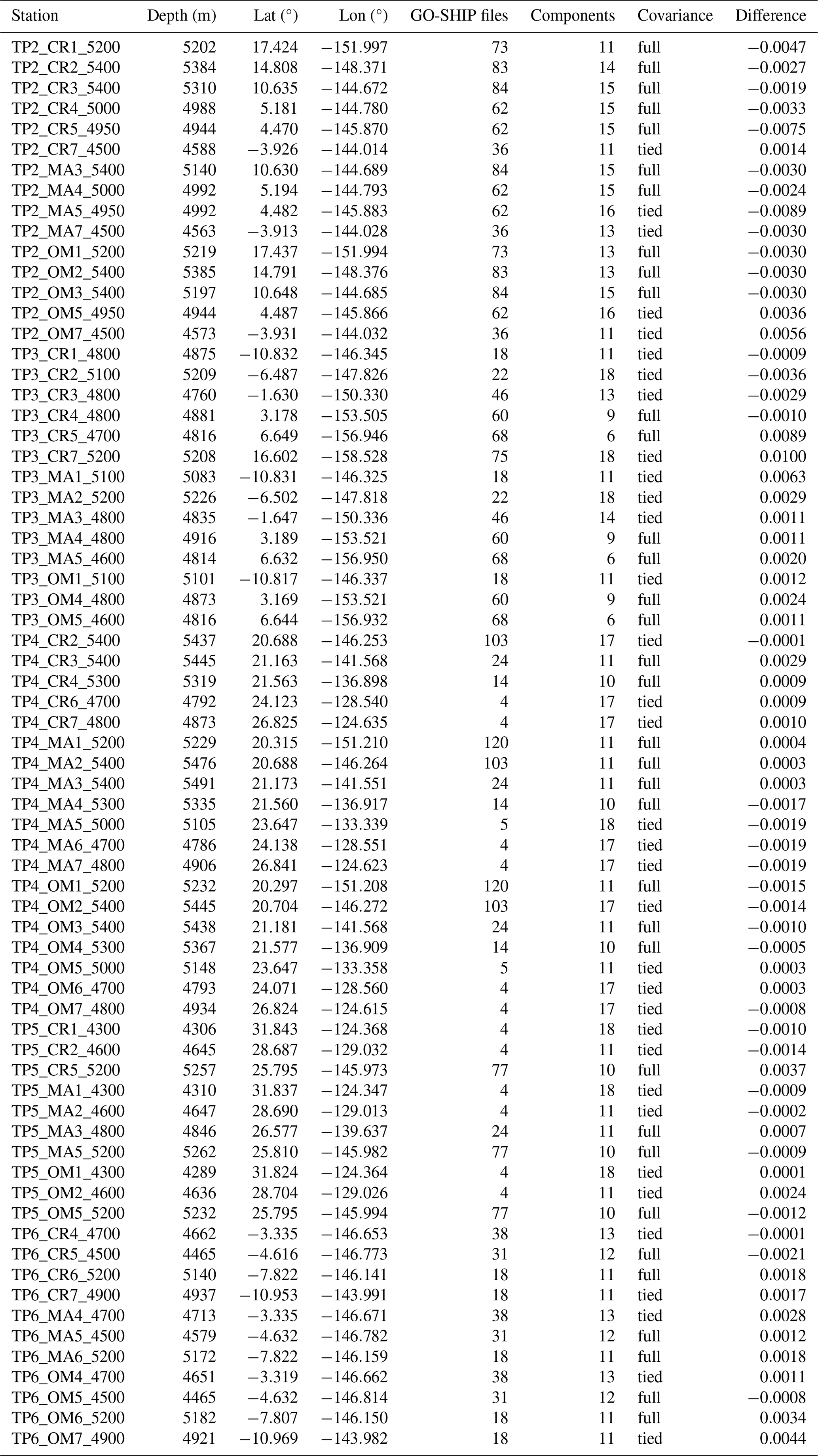
The Trans-Pacific Transit (TPT) Expedition occurred over six individual legs, with the duration of each leg approximately 21 d, between June 2023 and January 2024 on Research Vessel (R/V) Dagon (Jamieson et al., 2024). The vessel covered 20° longitude and 30° latitude over the central and eastern abyssal Pacific Ocean, including the Molokai and Clarion Clipperton fracture zones (Fig. 1). Bathymetry and backscatter intensity data were acquired throughout the expedition using a hull-mounted Kongsberg EM124 multibeam echosounder. At each site, three autonomous landers were deployed in a roughly 2 km equilateral triangle, acquiring a total of 73 surface-to-seafloor profiles of temperature and pressure (at a frequency of 2 Hz secured to the landers). These data are referred to here as “TPT profiles”. Conductivity, temperature and depth (CTD) sensor profiles from repeat Global Ocean Ship-Based Hydrographic Investigations Program (GO-SHIP) hydrographic sections, P16 and P02, provided observations within the study regions along meridional and zonal transects, respectively (see locations in Fig. 1). The GO-SHIP sections were used in two ways: first, they were used to complete Gaussian mixture modelling (GMM), which was applied to the TPT profiles to generate modelled practical salinity (SP) profiles (see Methods section on GMM); second, they provided additional locations to derive the bottom mixed layer (BML) thickness. The BML derivation, followed by a random forest regressor, was applied to the GMM-derived TPT profiles and GO-SHIP profiles as one dataset and is detailed in the following sections.

2.1 Data collection

Three autonomous landers, Magna, Omma and Cranch included a baited camera system, Niskin bottles and a CTD sensor measuring at 1 or 0.1 Hz (SBE49 FastCAT, SeaBird Electronics, Bellevue, WA). The landers descended at an average speed of 0.8 m s⁻¹, spent up to 8 h on the seafloor, and then returned to the surface by releasing their ballast weights via an acoustic modem. On legs two to six, there was the addition of a temperature (t) and pressure (p) logger (RBRduet|deep) mounted to the lander frame measuring at 2 Hz with an accuracy of ±0.002 °C and 0.05 % full-scale respectively (RBR, 2024). Due to the consistent high-frequency measurements of the t–p sensors, and the inconsistent data collection of the CTDs, we have used the t–p logger data and applied GMM to the profiles (see the following section). The Niskin bottles collected a water sample on the seafloor, which was analyzed with an 8400B Autosal Salinometer providing a bottom water practical salinity (SP) value. Leg one data was omitted from this study due to no t–p loggers, and a total of 69 profiles were suitable for this study. The exact locations of deployments are in Table A1.

GO-SHIP profiles were obtained through the CLIVAR and Carbon Hydrographic Data Office (CCHDO, https://cchdo.ucsd.edu/, last access: 24 November 2024) for repeat hydrographic Sects. P02 and P16 which form part of the GO-SHIP program. These were voyage numbers: 31WTTUNES_3, 325020060213 and 33R0150410 for P16 and 49K6K9401_1, 318M200406 and 318M20130321 for P02. Only profiles that exceeded 2000 m and reached within 40 m of the metadata bottom depth were used to calculate the BML thickness. Only one occupation along line P16 went north of 23° N, therefore north of this latitude was excluded for line P16. A gridded version of GO-SHIP dataset, GO-SHIP Easy Ocean provided by Katsumata et al. (2022), and available from https://doi.org/10.5281/zenodo.13315689 (Katsumata et al., 2024) was used to produce the background neutral density, γ_n, and conservative temperature, θ, for Figs. 5 and 6.

2.2 Gaussian mixture modeling in Θ-p-SA space

Gaussian mixture modeling applications (GMM) can achieve unsupervised classification of the water column, identifying coherent patterns in the associated domains (Maze, 2017).

In three-dimensional space (Θ-p-SA), the abyssopelagic zone occupies a relatively small volume (Hjelmervik and Hjelmervik, 2014; McDougall and Jackett, 2007). For hydrographic profiles close in proximity, this space is even tighter (McDougall and Jackett, 2007). Considering this, gaussian mixture modeling applications (GMM) can be applied to automatically group variables of the water column into a distinct number of components, like clusters, revealing consistent patterns in the data (Maze, 2017). GO-SHIP profiles in the study region (detailed in Sect. 2.1) were used to predict practical salinity (SP) from 2500 m to the seafloor. Only profiles collected within the last 5 years and within 10° latitude and 10° longitude that exceeded 2000 m were used for each site (Pedregosa et al., 2011; Maze, 2017). To predict SP for each TPT temperature and pressure profile. Model selection used information-theory criteria, focusing on the covariance type and number of components in the model using the Gaussian Mixture scikit-learn Python package (Pedregosa et al., 2011). The maximum number of components was limited to 21. The covariance types were limited to each component having its own general covariance matrix or all components sharing the same general covariance matrix. The elbow method was used to determine the number of components in the model with a brief examination of the BIC value (Table A1). If the modeled SP output was physically unstable, the next best option was chosen. The modeled SP was compared with the measured SP from a seafloor water sample analyzed on the vessel using an 8400B Autosal Lab Salinometer (Table A1) with negligible differences found. A further detailed explanation and model details for each TPT profile are provided in Table A1.

2.3 BML thickness derivation

Several methods exist for determining the BML thickness, as with the surface mixed layer thickness. The threshold method (TH) uses the depth at which the difference to the seafloor in either Θ or σ₄, potential density referenced to 4000 dbar in this case, is less than a defined threshold value. These values range from 0.02 °C (Lentz and Trowbridge, 1991), 0.001 °C (Hogg et al., 1982), 0.005 °C (Lozovatsky and Shapovalov, 2012) to $\mathrm{6}\times {\mathrm{10}}^{-\mathrm{4}}$ kg m⁻³ (Perlin et al., 2005). We used a threshold value of 0.003 °C for the region. This value was chosen as it provided the highest mean quality index (QI) for the BML thickness (1) for all the TPT profiles when comparing threshold values of 0.001, 0.002, 0.003, 0.004, and 0.005 (Appendix B). A quality index was initially defined by Lorbacher et al. (2006) as a value between 0 and 1 capturing the conservative temperature variability in 1.5 times the BML thickness compared to the variability over the BML thickness. In equation form:

$$\begin{array}{}\text{(1)}& {\text{QI}}_{\text{BML}}=\mathrm{1}-{\displaystyle \frac{A\mathrm{1}}{A\mathrm{2}}}=\mathrm{1}-{\displaystyle \frac{\mathit{\sigma }({\mathrm{\Theta }}_n-\langle \mathrm{\Theta }\rangle ){|}_{\left(h_{\text{BML}}\right)}}{\mathit{\sigma }({\mathrm{\Theta }}_n-\langle \mathrm{\Theta }\rangle ){|}_{(h_{\text{BML}}\times \mathrm{1.5})}}}\end{array}$$

where σ() is the standard deviation from the vertical mean 〈〉 conservative temperature from h_BML. h_BML is the BML thickness (Lorbacher et al., 2006; Huang et al., 2018a).

The threshold-gradient method (GR) is also used (Banyte et al., 2018; Weatherly and Martin, 1978). We defined this method as the thickness at which $\mathit{\delta }{\mathit{\sigma }}_{\mathrm{4}}/\mathit{\delta }z$ over 20 m intervals is less than a criterion of $\mathrm{1}\times {\mathrm{10}}^{-\mathrm{3}}$ kg m⁻³ (Banyte et al., 2018), making the minimum BML thickness 10 m.

Several techniques have been put forward over the last decade, including a relative variance (RV) method (Huang et al., 2018b), split-and-merge algorithms (Thomson and Fine, 2003) and an integrated method (Huang et al., 2018a) that combines several methods together. We included the RV method and the Douglas–Peucker (DP) algorithm method. The RV method relies on calculating the ratio between the standard deviation and the greatest variation of Θ or σ above the seabed. The location where the least relative variance occurs is identified as the upper boundary of the BML. The RV method is available through the original research (Huang et al., 2018b). The DP method is a split-and-merge technique that has been previously adopted to calculate the surface mixed layer (Thomson and Fine, 2003). The DP algorithm estimates a given profile by using a series of simplified line segments that represent large changes in slope or any abrupt changes in the profile. Therefore, the lowest part of the segment belongs to the BML. The DP algorithm is available within MATLAB and requires a ϵ value between 0 and 1 to determine the number of line segments (Ahmadzadeh, 2017). We included 0.002 and 0.008 as two possible DP methods (DP2 and DP8, respectively) (Appendix B).

The integrated method put forward by Huang et al. (2018a) focuses on the use of multiple methods (TH, the curvature method, Lorbacher et al., 2006; the maximum angle method, Chu and Fan, 2011, and RV, Huang et al., 2018b), calculating the QI for each method, and then choosing the BML thickness with the highest QI (Huang et al., 2019). Relying on QI-based selection of BML thickness from multiple methods produced highly variable results, even across nearby locations (within 3 km). That is not to say this variation may not be real, but visual inspection was still needed to assess accuracy, and the variation was not consistent with global maps from either Banyte et al. (2018) or Huang et al. (2019). Therefore, unlike Huang's global integrated approach, the single threshold method that produced consistent results was more appropriate for our regional study, avoiding unnecessary and possibly unreal variability that ultimately required manual validation.

The suitability of the threshold value, despite sometimes having a lower QI, is shown in Fig. 2 at different locations with additional annotation in Fig. 2c. At times, the QI did capture the BML thickness values that were unusable (e.g. small RV QI values in Fig. 2f). However, on the upper scale, the highest QI value could provide an unlikely, significantly larger BML thickness than where the density gradient approached zero and appeared visually correct. For example, in Fig. 2c for the profile on the left side, the highest QI was 0.78 and far from the visual BML thickness height. Considering all TPT and GO-SHIP profiles, consistency in the average values of each method (Fig. 4) and their performance when assessed visually (Fig. 2), using the threshold method consistently over the whole dataset, provided the most reasonable result.

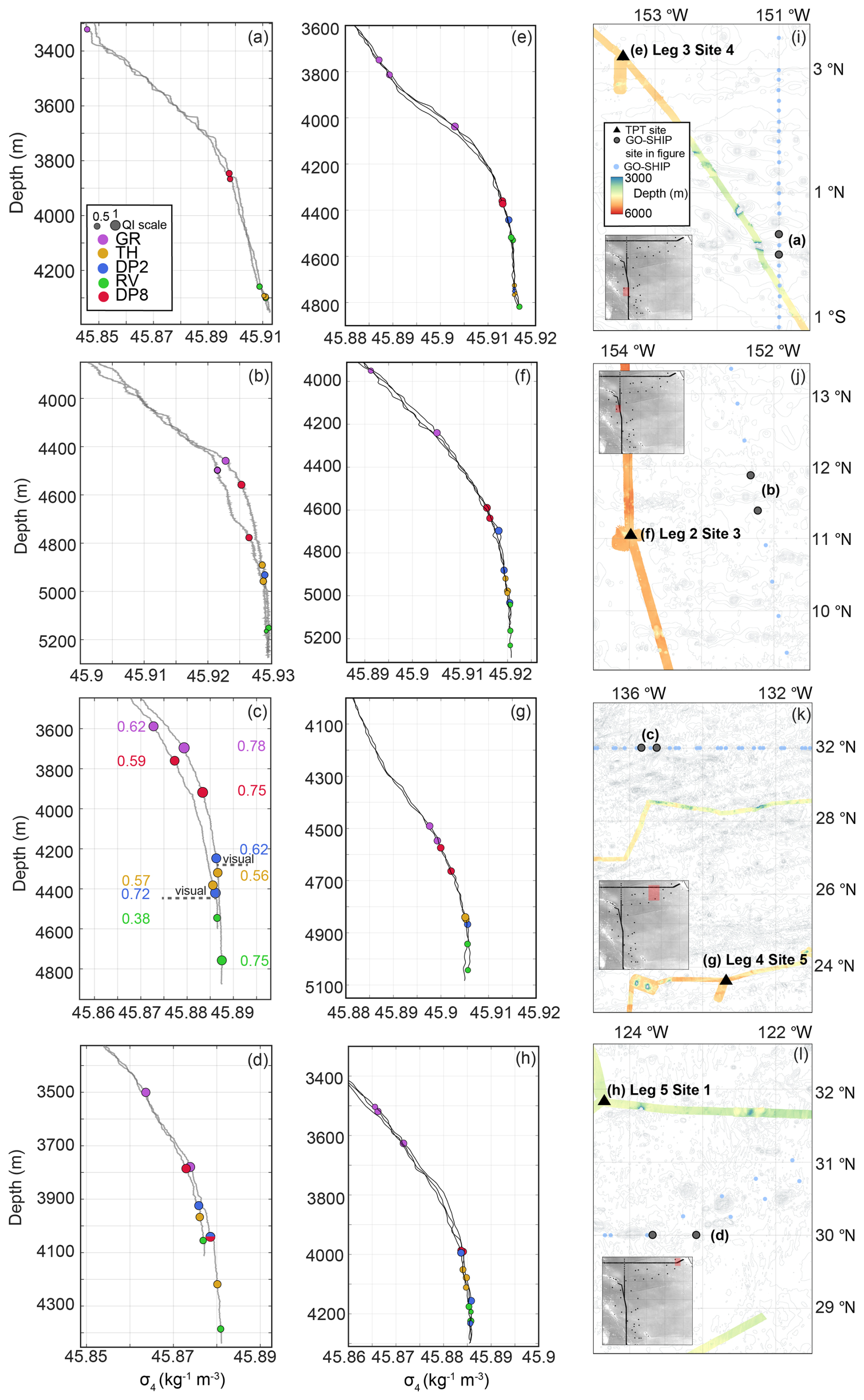
Figure 2 Example profiles of σ₄ and BML thickness outputs from (a)–(h). Color and size of the marker correspond to the method and the quality index (QI) of the BML (a). The map and inserts in (i)–(l) detail the locations of the profiles shown in the respective subplot. Grey map shows the study region with GEBCO bathymetry and sites (key in i; see Fig. 1 for more detail), the red region the extent of the figure and black points indicating all profiles used. Blue circles are GO-SHIP, with light blue indicating profiles used but not displayed, and black triangles are TPT locations. (a) P16 GO-SHIP profiles in 2002 between 0 and 0.5° N and (b) in 2015 between 12 and 13° N, (c) P02 GO-SHIP profiles in 2022 between 135 and 136° W and (d) in 2022 between 124 and 123° W. (e) TPT voyage Leg 3 Site 4, (f) Leg 2 Site 3, (g) Leg 4 Site 5, and (h) Leg 5 Site 1. Panel (c) includes a line of visual interpretation and the exact values of the quality index, as also indicated by the marker size at the BML thickness for each method.

2.4 Random Forest Regression

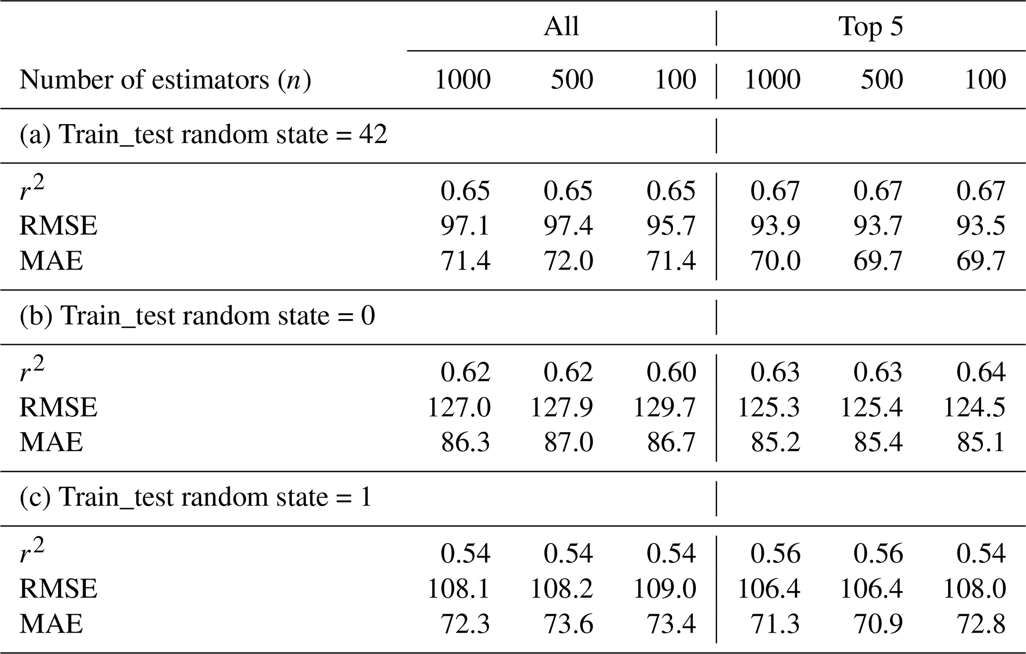
We considered bathymetric parameters (terrain roughness index (TRI) and slope) and dynamic parameters (internal tide energy dissipation and depth) within a Random Forest Regressor (RF) to disentangle patterns in the BML thickness. Machine learning techniques have been used to estimate the surface mixed layer depth, however this the first time it has been applied to the BML (Imchen et al., 2025; Foster et al., 2021). The RF machine learning technique, included as the RandomForestRegressor scikit package in Python (Pedregosa et al., 2011) is a ensemble machine learning estimator that combines the outputs of multiple decision trees to increase predictive accuracy and control overfitting. Each decision tree is trained on the dataset using a bootstrap aggregation technique, and the final prediction is obtained by averaging the outputs for regression (Carvalho et al., 2019; Imchen et al., 2025). We randomly selected 80 % of the dataset to build each tree and the remaining 20 % of the dataset to test the model using train_test_split within scikit (Pedregosa et al., 2011). We modified the number of trees from 100 (default value) to 500 and 1000 for sensitivity testing (Table 1) with the random state of the train_test_split at 42, 0 or 1. The number of trees did not add significant computing time or signficantly alter the results, therefore we maximised the number of trees at n=1000 to further test different random subsets of the data with train_test_split then changed between 42, and 0 to 7. The random state was kept at 42 for the RF for all itterations.

Table 1 Random Forest performance for different numbers of estimators (n), comparing models trained on all features vs. the top five features.

As discussed in the Data Collection section, internal tide energy dissipation (W m⁻²) for all (M2, S2 and K1) tidal constituents broken down into dissipation processes; low-mode wave-wave interactions, low-mode scattering by small-scale topography, low-mode interaction with critical slopes, low-mode shoaling and local dissipation of high modes was accessed through the paper by de Lavergne et al. (2019). These variables, alongside slope and TRI were chosen based on their accessibility and relevance to BML thickness (Ruan et al., 2017; Gula et al., 2016; Liu et al., 2023). Depth is a known contributor to the BML thickness (Huang et al., 2019; Lozovatsky and Shapovalov, 2012) as are bathymetric variables of slope and TRI (Armi and Millard, 1976; Wunsch, 1970; Polzin and McDougall, 2022). The relative contribution of tidal dissipation mechanisms near the seafloor, therefore influencing the BML thickness has been discussed in literature (de Lavergne et al., 2019). When internal waves hit the seafloor, they lose energy through either scattering off small rough spots and losing energy, or reflecting or shoaling off topographic features, depending on their shape and height (St. Laurent et al., 2001; Müller and Xu, 1992). These processes, along with others that are not as well understood, like wave capture and scattering by mesoscale eddies Bühler and McIntyre (2005), Polzin (2008), Mathur et al. (2014), can speed up the dissipation of tides and change the thickness of the bottom mixed layer. A grid point from each of the dissipation parameters was assigned to each GO-SHIP and TPT point using cKDTree in scipy for nearest-neighbor lookup (Virtanen et al., 2020). This method constructs a binary space-partitioning tree applying axis-aligned hyperrectangles via the sliding midpoint rule (Maneewongvatana and Mount, 1999). This provides efficient nearest-neighbor queries by recursively improving the search space across coordinate axes to determine the nearest latitude and longitude grid point to the GO-SHIP and TPT observations.

Bathymetric variables (TRI, and slope) were compiled from the latest GEBCO 2024 Grid, including the standard deviation (GEBCO Compilation Group, 2024). TRI and slope were calculated using the ArcGIS Geomorphometry & Gradient Metrics toolbox with a neighbourhood of 9×9 cells (Evans et al., 2019). TRI is a useful derivative of bathymetric and topographic datasets in order to enable quantification of the spatial heterogeneity of the surface under investigation (Riley et al., 1999). The TRI metric can be a valuable analytical tool for understanding the effect of landscape on processes, geomorphological evolution, and for habitat mapping and modeling regimes. For the extent of the study region (Fig. 1) the slope and TRI were calculated at buffer zones of 25, 50, 100 and 200 km (Fig. B3). At each GO-SHIP and TPT data point, the TRI was extracted to assess the variation for different buffer zones. The RF was completed with the 50 km buffer, as the resolution for the dissipation values was 50 km. The depth for the GO-SHIP sites was taken as the “bottom depth” variable available in the datasets.

The GO-SHIP observations included multiple occupations as detailed in the Data collection section above. In some locations the exact latitude and longitude was covered in multiple years, although this is not spatially consistent throughout the observations. The profiles over the different occupations provide different BML thicknesses, however it is impossible to deduce the reasoning behind the differences at these yearly timescales as we know the BML thickness may change within a matter of hours (Weatherly and Martin, 1978; Chen et al., 2023). For this reason, we clustered the GO-SHIP observations within the RF using dbscan in scikit (Pedregosa et al., 2011). Geographic clustering was performed by converting the GO-SHIP latitude and longitude coordinates to radians and applying dbscan with a haversine metric and a 3 km neighborhood radius to group nearby data points. For consistency between the TPT and GO-SHIP sites, TPT sites within a 3 km radius of one another (each leg and site) were averaged and GO-SHIP sites were averaged based on the 3 km neighborhood radius from dbscan. Because the TPT SP values were corrected using nearby GO-SHIP profiles, the combined dataset may inherit some spatial imbalance towards the more regularly sampled GO-SHIP sections; however, both datasets occupy the same hydrographic regime and spatial scale, making them appropriate for joint analysis while acknowledging that this imbalance could introduce minor bias in the RF feature relationships.

3 Results

3.1 BML thickness

The average and median thickness of the BML using the TH method for all data points in the abyssal study region was 240 and 176 m respectively, and the standard deviation was 200 m (Fig. 3). The BML was inhomogeneous over the region, its thickness decreasing around continental slope regions approaching Mexico and the southern part of Hawaii. Between 15° S and 2° N the BML was below 200 m. There was a distinct change between 2 and 15° N where the BML approximately doubled and reached a maximum of 799 m crossing the Clarion Fracture Zone before decreasing to below 90 m south of Hawaii. Along the zonal section of P02, the BML exhibited an approximately 50 % increase between 135 to 130° W and decreased to approximately 100 m on approaching the continental slope. The TPT expedition data indicated generally similar patterns as the repeat hydrographic sections. These patterns excluded Leg 4 Site 7, where the BML was the largest of the TPT sites (Fig. 3).

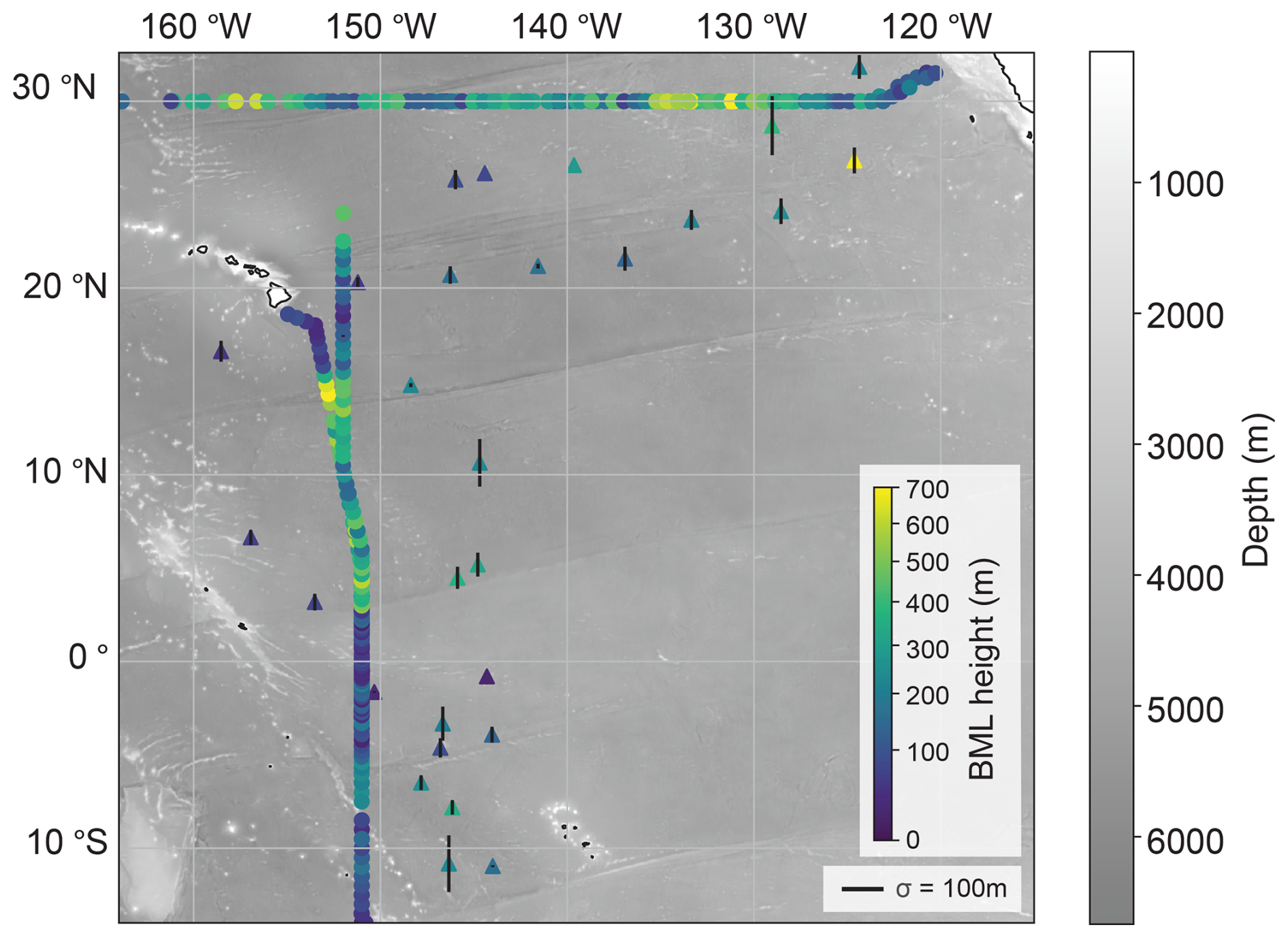
Figure 3 Bottom mixed layer (BML) thickness (m) derived from the threshold method (TH). It is calculated using the TPT Expedition profiles (triangles) and GO-SHIP profiles (circles). The TPT profiles are within 3 km of each other and therefore a standard deviation is included.

To provide insight into the efficacy of the derivation methods, we calculated a QI (Lorbacher et al., 2006) for each profile and its five possible BML thickness values (Fig. 4). Visual inspection of the BML thickness estimates and their associated QI indicated that a higher QI and lower standard deviation do not always provide confidence in the BML value. TPT profiles within 3 km of each other in Fig. 2e had a higher QI for the GR and DP8 methods; however, the methods estimated very different BML thicknesses for very similar profiles. In contrast, the TH method, with lower QI values, was consistent among the profiles and appeared to capture the position of profile change under contrasting abyssal conditions sufficiently. For example, across all Fig. 2e–h the TH BML thicknesses were in close proximity to one another. Additionally, the TH thickness corresponded with the visually identifiable thickness, despite the GR values being close in value to each other and of a high QI (Fig. 2c). We therefore chose the TH method for all BML thickness values going forward due to its dependable performance when applied to both TPT and GO-SHIP profiles over different regions in the study area.

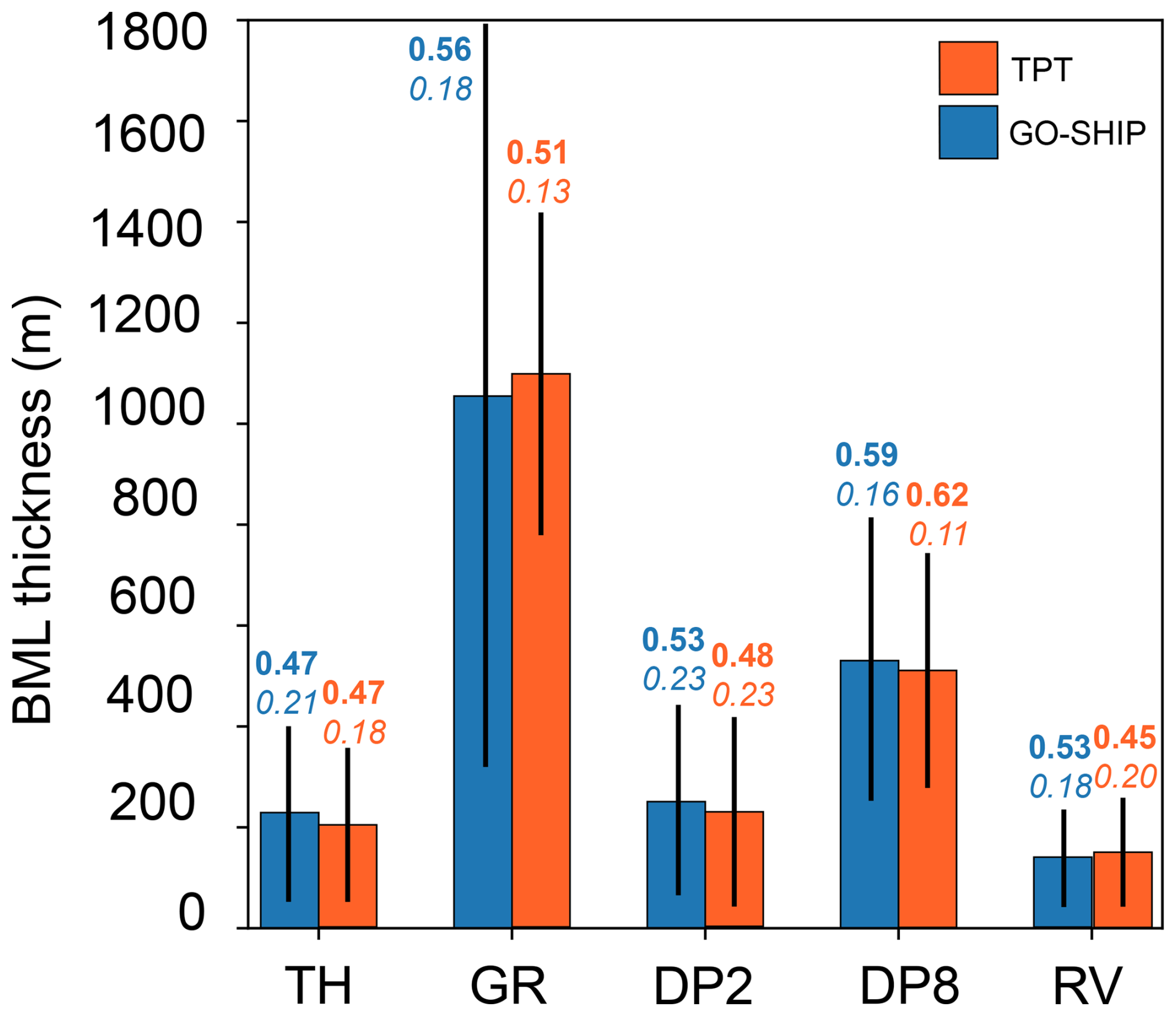
Figure 4 Average bottom mixed layer (BML) thickness (m) for the threshold method (TH), gradient method (GR), Douglas–Peuker method using an ϵ of 0.002 (DP2), Douglas–Peuker method using an ϵ of 0.080 (DP8) and the relative variance method (RV). The BML thickness is calculated using the TPT Expedition profiles (orange) and GO-SHIP profiles (blue) with the length of the line indicating the range of the thickness. Bold values above the bars are the mean quality index (QI) and the italicised values are the standard deviation of the QI.

3.2 Spatial variability

On meridional transect P16 between 4 and 16° N, depths are over 5000 m, and the BML thickness was at its greatest along the transect (Fig. 5). The transition regions at 4 and 16° N appear to have the widest variation in BML over the different occupations. The TRI was low over the majority of this region, with increases near the Hawaiian Islands, over the Boudeuse Ridge (10° S) and other prominent seafloor features visible in the bathymetric data (Fig. 7b and c). Similarly, the TRI reached a maximum across transect P02 when it crossed the Murray Fracture Zone and the Moonless Mountains before increasing towards the North American continental slope (see Fig. 1 for locations). TPT sites close to the major fracture zones and seamount chains had higher TRI and slope values over the 50 km buffer range and exhibited patterns connecting them to the P16 and P02 lines spatially. The P02 transect had a higher BML thickness (298 ± 170 m) compared to P16 (175 ± 157 m) (Figs. 5 and 6). Similar to P16, the sections of changes in BML thickness along P02 (>500 m from 136 to 129° W) broadly intersected with larger differences in BML thicknesses over the different occupations (Fig. 6).

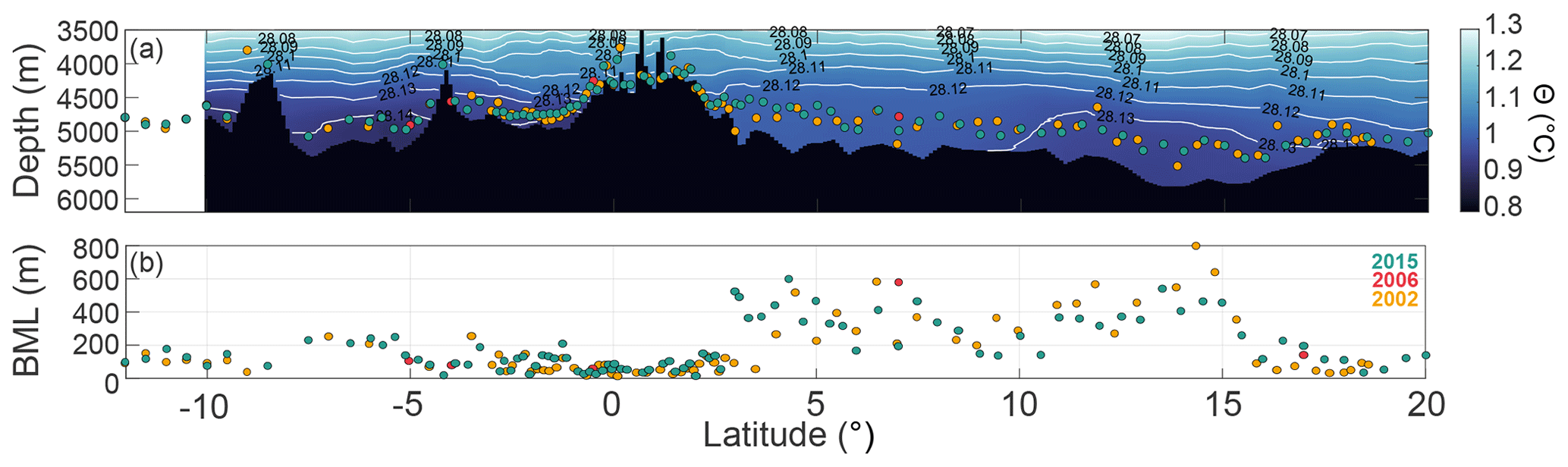
Figure 5 The P16 repeat hydrographic line nominally along 150° W with (a) conservative temperature (Θ) with neutral density (γ_n) as the white contours and the BML thickness for 2015 (green), 2006 (red), and 2002 (orange). Note the seafloor, Θ and γ_n are from the gridded data product available from Katsumata et al. (2022) and therefore may not be an exact representation of the seafloor depth, (b) BML thickness above the seafloor with color representation as in (a).

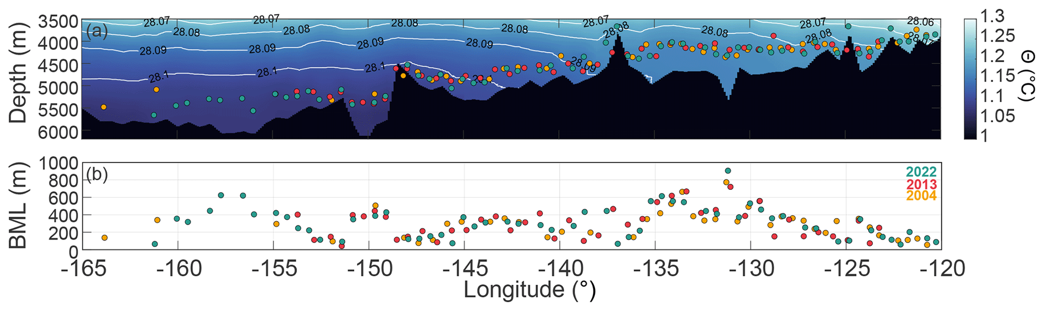
Figure 6 The P02 repeat hydrographic line nominally along 30° N with (a) conservative temperature (Θ) with neutral density (γ_n) as the white contours and the BML thickness for 2002 (green), 2013 (red), and 2004 (orange). Note the seafloor, Θ and γ_n are from the gridded data product available from Katsumata et al. (2022) and therefore may not be an exact representation of the seafloor depth, (b) BML thickness above the seafloor with color representation as in (a).

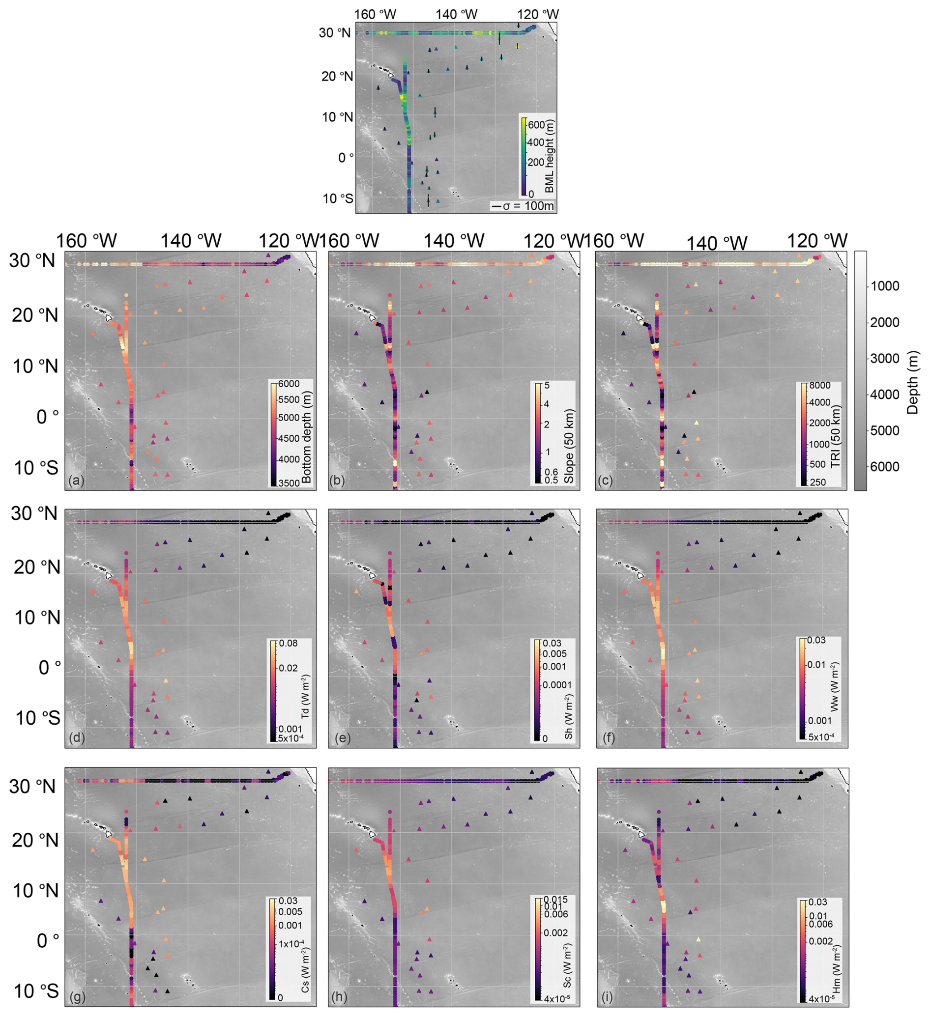
Figure 7 All GO-SHIP (circle) and TPT (triangle) site variables used for the Random Forest Regressor (RF). The top BML thickness figure is the same as Fig. 3 for reference. (a) Bottom depth (m), (b) slope over a 50 km radius (°), (c) terrain roughness index (TRI) over a 50 km buffer, (d) Td = total internal tide energy dissipation (W m⁻²), (e) SH = low-mode dissipation from shoaling (W m⁻²), (f) Ww = low-mode dissipation from wave-wave interaction (W m⁻²), (g) Cs = low-mode dissipation from critical slopes (W m⁻²), (h) Sc = low-mode dissipation from scattering (W m⁻²) and (i) Hm = high-mode dissipation from local processes (W m⁻²). Panels (d)–(i) are from de Lavergne et al. (2019). The background regional bathymetry is from the Global Multi-Resolution Topography (GMRT) Synthesis (Ryan et al., 2009) Released CC BY 4.0 Deep | Attribution 4.0 International | Creative Commons. Note the colour scale is different in (d) compared with (e)–(i).

3.3 Random Forest Regression

The TPT and GO-SHIP profiles were analysed together as part of a RF. As described in the Methods section, GO-SHIP data points within 3 km of one another were averaged together as a mean value to remove instances of temporal variability at unknown time scales. After the averaging, the number of GO-SHIP data points reduced from 335 to 301. The number of TPT data points was 29; therefore, a total of 330 points were used for the analysis. For each point, we extracted values of bottom depth (m), slope, TRI, and internal tide energy dissipation values of low-mode wave-wave interactions, low-mode critical slope, low-mode scattering, low-mode shoaling, high-mode (≥6) local dissipation and total internal energy dissipation which is a sum of all the losses from the five processes (in W m⁻²) (Fig. 7). The dissipation parameters are defined in depth by de Lavergne et al. (2019).

The feature with the highest importance score (∼0.4) across all iterations of the RF was the bottom depth. For each variation of train test split sample data (i.e. random_state=42, 0 or 1) chosen to train the RF, the same features with the highest importance were in the top 3. In order, these were the bottom depth, total dissipation and slope. The number of iterations (n=1000, 500 or 100) and the three most commonly used train test split values (random_state=42, 0 or 1) were sensitivity tested due to the relatively small number of data points. Reducing the predictor variables to include only the top 5 features, ranked by importance, increased the correlation coefficient, r², by ∼0.02, regardless of the number of iterations or the random_state value (Table 1). Similarly, the root mean squared error (RMSE) and mean average error (MAE) reduced an insignificant amount (∼2 m) when including only the top 5 features (Table 1). The results from n=1000, 500 or 100 had comparable feature importance scores; therefore, only the results from n=1000, all features and additional train test split values of random_state=42, 0–7 were run and are shown in Figs. 8 and 9. If we were to keep the random_state value as empty, which is the default, the sensitivity in altering the number of iterations would not be effectively tested. Train test values of random_state=42 and 0–7 were completed for n=1000 with the r² and RMSE displayed in Fig. 9. The nine sets of the RF residual model outputs are shown in Fig. 9. The r² was between a minimum of 0.53 and a maximum of 0.77 and the RMSE had a minimum of 87.1 and a maximum of 127.

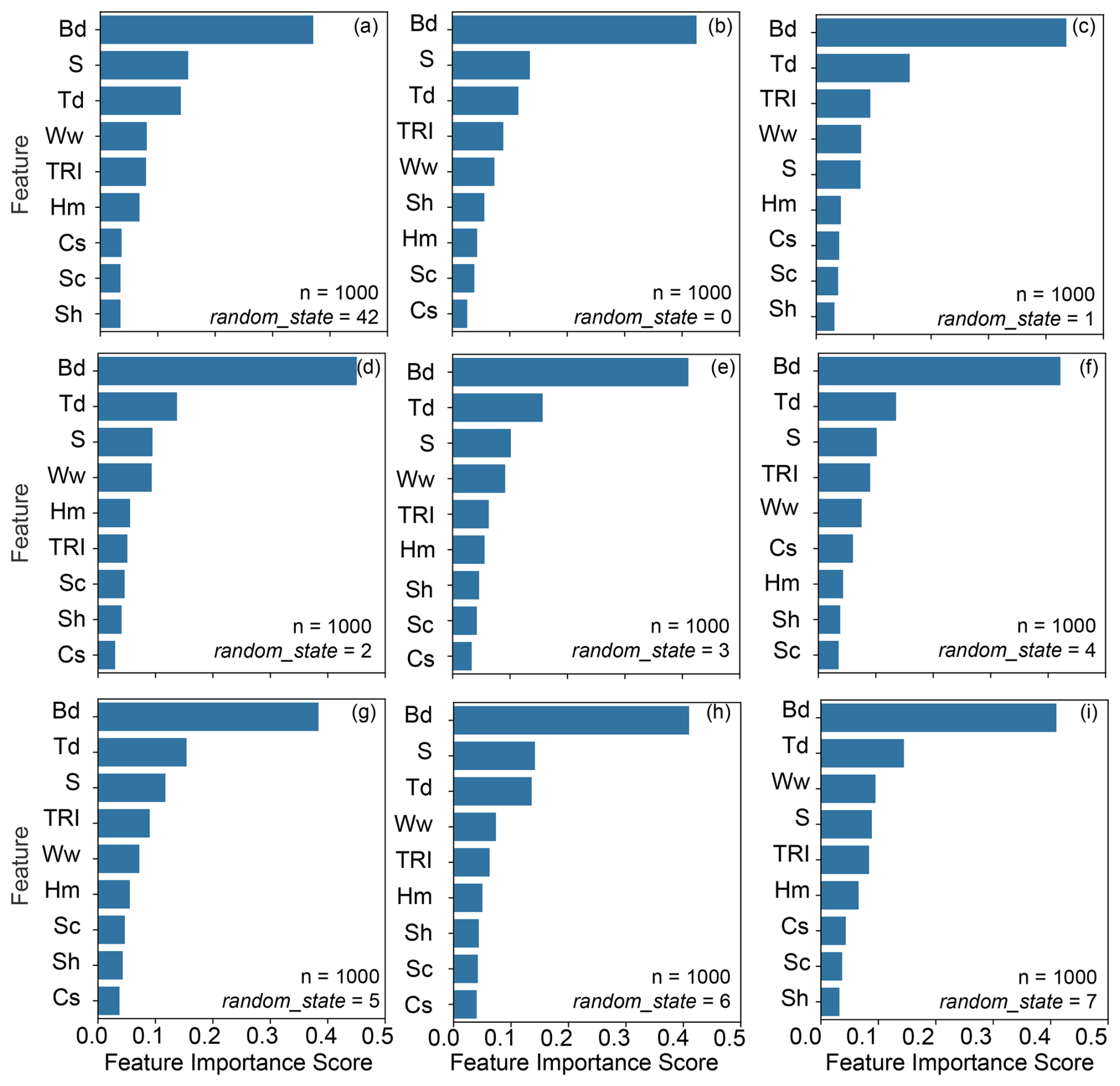
Figure 8 Feature importance scores for each feature output from the number of iterations (n)=1000 for the train test split random_state values of the 80–20 data split for (a) 42 and (b–i) for 0–7 for the Random Forest Regressor. Bd = bottom depth, S = slope, TRI = terrain roughness index, Td = total internal tide energy dissipation, Sh = low-mode dissipation from shoaling, Ww = low-mode dissipation from wave-wave interaction, Cs = low-mode dissipation from critical slopes, Sc = low-mode dissipation from scattering and Hm = high-mode dissipation from local processes.

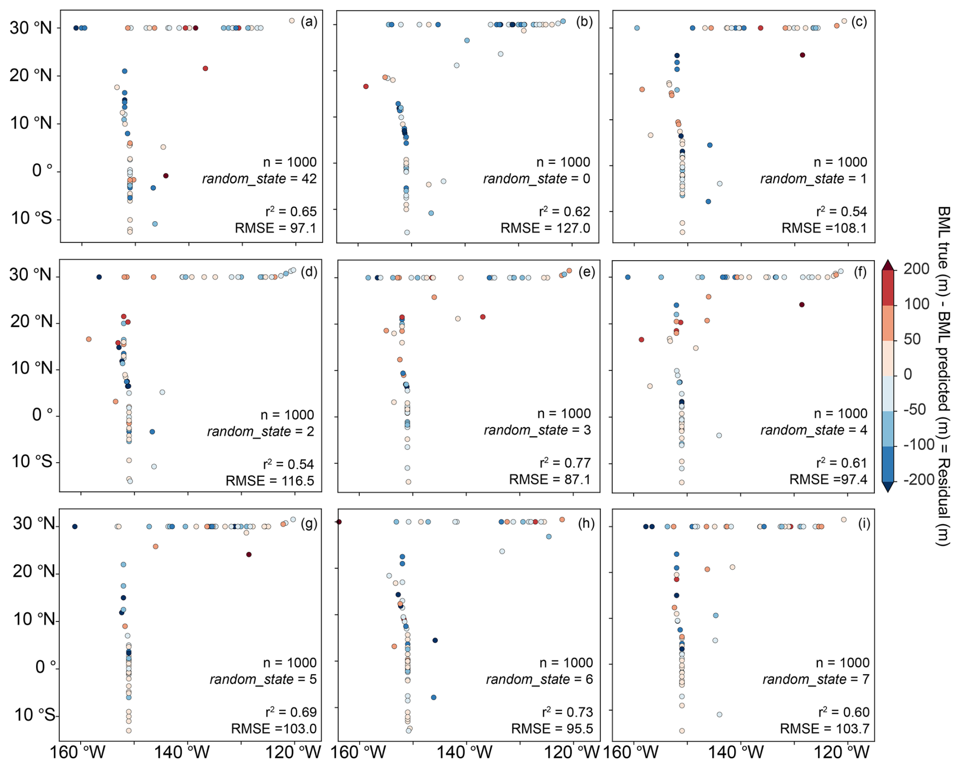
Figure 9 Spatial plots of the BML residual (m) (BML true–BML predicted) for the train test random_state values used to train the Random Forest Regressor with the number of iterations =1000, generating a spread of the data for random_state equal to (a) 42 and (b–i) for 0–7. The correlation coefficient and the Root Mean Squared Error (RMSE) is displayed on each figure.

The different random_state values changed the ranking order of the feature importance scores, however the same features were within the top five, with the bottom depth always the highest. The slope and TRI are intrinsically linked due to their calculation from the same bathymetric dataset, with slope quantifying the local gradient over a 50 km radius and TRI capturing the variability within a neighborhood, averaged over a 50 km radius aligning with the spatial resolution the dissipation values, a 0.5° grid size. A surface may be steep but smooth, or flat yet jagged, drawing not always a strong correlation between the two. For example, there are sharp changes latitudinally, however, both TRI and slope are high and more gradual along the P02 line as part of the broad sloping region from the continental slope of Mexico to the center of the Pacific Ocean (Fig. 7b and c). The western end of the P02 line has higher internal tidal dissipation compared to the more eastern half due to the presence of the Hawaiian Islands (Kelly et al., 2010). The full spatial extent of the dissipation parameters, not just at our data points, at 0.5° resolution are displayed and explained in de Lavergne et al. (2019). Overall, the internal tidal dissipation for each low-mode process (Fig. 7e–h), and the total dissipation (Fig. 7d), is highest between Hawaii and just north of the equator, intersecting with the region of higher BML along P16 aside from 15–20° N next to the Hawaiian Islands, where the BML decreases. This decrease overlaps with a slight decrease in bottom depth (Fig. 7a).

4 Discussion

Density profiles over the central and eastern Pacific Ocean provide an inhomogeneous outlook of BML thickness variations at abyssal depths across plains and topographic features. Basin-scale expeditions such as the TPT voyages are frequently multidisciplinary in scope, with competing demands on vessel time. Incorporation of these profiles with the repeat GO-SHIP profiles provides increased understanding of the BML. Using RF methods, we found that bottom depth, total internal tide dissipation and slope are the highest-performing features to predict the BML thickness in this region. Because several predictors share spatial structure (e.g., bottom depth and total dissipation), the RF highlights associations rather than uniquely isolating independent physical drivers, and this limitation should be considered when interpreting the feature importance results (Strobl et al., 2008).

In the central and eastern Pacific abyssal ocean, the thickness of the BML was inhomogeneous with an average value of 226 ± 172 m. The BML was calculated using the (Θ) profiles through the threshold method (0.003 °C) for the study region. There is no accepted standard methodology for calculating the BML thickness. It often depends on user-defined numerical values within those methods and depends on the region of interest. The integrated method proposed by Huang et al. (2018a), was used to calculate the BML depth globally, providing an average Pacific Ocean BML thickness of 64 m (Huang et al., 2019). We found that for our abyssal ocean context, using an integrated approach that combines multiple methods and calculates a QI to get the highest “quality” BML thickness generated spurious results for profiles within three kilometres of one another, making it difficult to compare BMLs estimated with different methods. Although the QI was calculated, visual interpretation was necessary to confirm the results, mirroring the approach taken within the integrated method where visual identification was still needed (Huang et al., 2019). The variability in BML thickness is not unexpected given the variation in topographic features across the region, likely changes in friction velocity, and a wide longitudinal and latitudinal range (Weatherly and Martin, 1978; Kunze et al., 2012). Profiles from the TPT Expedition broadly followed the same spatial patterns as those from the hydrographic sections and show similar spatial variations in BML thickness as Banyte et al. (2018).

In all instances, the RF identified the bottom depth, slope, total internal wave energy dissipation, TRI and low-mode wave-wave interactions as the most important predictors of the BML thickness in this Pacific Ocean abyssal setting. These results are physically intuitive, with the bottom depth constraining the maximum possible BML thickness, background stratification and the vertical extent available for turbulent mixing, which is consistent with past research (Laurent and Garrett, 2002; Liu et al., 2023; Lozovatsky and Shapovalov, 2012). Importantly, dissipation patterns in the de Lavergne et al. (2019) dataset are not set by depth, but by the distribution of internal tide energy sources, scattering pathways, and nonlinear wave–wave losses. Deep basins may accumulate low-mode energy and therefore show elevated dissipation, but this reflects remote energy propagation and decay rather than a mechanistic link to depth itself. Therefore, even where depth and dissipation appear spatially aligned in our RF model, this similarity arises from shared basin-scale structure rather than depth acting as a direct driver of turbulent energy loss.

The total internal wave energy dissipation value aggregates all internal tide dissipation mechanisms that drive turbulence (de Lavergne et al., 2019). On abyssal plains, where local topographic features are sparse, a substantial amount of this energy would likely originate remotely and dissipate gradually through sustained mixing events (Nikurashin and Legg, 2011). Therefore, the inclusion of low-mode wave-wave interactions as a predictor is especially significant. This variable refers to nonlinear energy transfers among long-wavelength internal tides. In regions with high low-mode wave-wave dissipation, this could lead to persistent near-bottom mixing that expands the BML thickness. This suggests that the BML thickness on the abyssal plain is of remote and sustained forcing origin, rather than high-mode breaking events (de Lavergne et al., 2019; Melet et al., 2013). Although the study region lies predominantly within the abyssal plain, the terrain is not uniform. As shown by Harris et al. (2014) and Fig. 7b and c, the region is interspersed with multiple features of abyssal plains, abyssal hills, and seamounts, creating heterogeneity in the TRI and slope. The observations north of Hawaii highlight where higher TRI and slope intersect with the smallest values of total internal tide dissipation and low-mode wave-wave interactions.

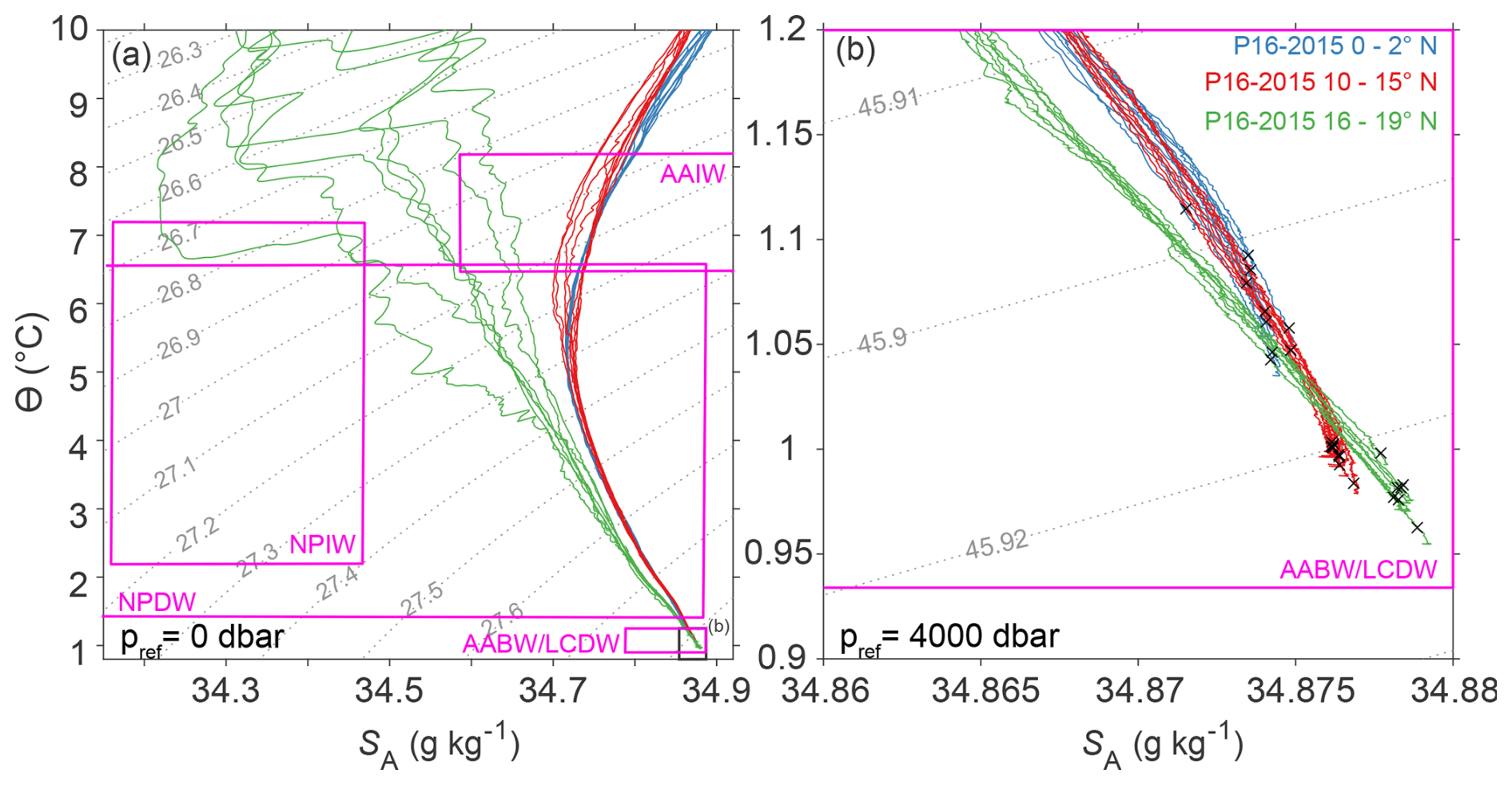
Figure 10 Conservative temperature (Θ, °) – Absolute Salinity (SA, g kg⁻¹) plots for latitudinal sections of the P16 line for the 2015 occupation between 0–2° N (blue), 10–15° N (red) and 16–19° N (green). (a) Wider portion of the water column with the (b) limits outlined. In (a) the dashed contour lines show the potential density referenced to the 0 dbar (σ₀) and in (b) the dashed lines show the potential density referenced to 4000 dbar (σ₄). Θ-SA North Pacific water mass properties are shown in magenta (Fuhr et al., 2021) and the BML for the profile is displayed with a black X. NPIW = North Pacific Intermediate Water, AAIW = Antarctic Intermediate Water, NPDW = North Pacific Deep Water, AABW = Antarctic Bottom Water, used here interchangeably with Lower Circumpolar Deep Water (LCDW). Displayed and calculated with the TEOS-10 toolbox (McDougall and Barker, 2011).

The TRI captures local bathymetric complexity at 50 km scales, which enhances bottom drag and internal tide scattering, even where mean slopes may be weak, supporting thicker BMLs by maintaining sustained and patchy mixing close to the boundary layer (Nikurashin and Ferrari, 2011; Nash et al., 2007). The slope of the topography within our study region is primarily of a subcritical regime; therefore, internal tides will refract and reflect weakly, allowing for persistent low-mode energy to mix over broader regions, rather than localized mixing. Between 4 and 15° N there is a small region where the low-mode critical slope dissipation increases (Fig. 7g), and the BML thickness is large, suggesting the critical slope may be more important here. Nested within the same region is the highest total dissipation of the study region (4–7° N) where there is high local high-mode dissipation, low-mode wave-wave interactions and low-mode critical slope dissipation. The TRI and slope are small over this region, culminating in the BML thickness being slightly above the average. Similar connections to the slope and the TRI have been identified in the North Atlantic Ocean and the South China Sea (Lozovatsky and Shapovalov, 2012; Liu et al., 2023).

Our results have highlighted differences in what factors drive the BML. Despite limited and sparsely located data points, it is clear that the BML thickness is a culmination of processes, both local and remote. The limited and spatially inconsistent data points meant we were unable to further the model to predict the BML without the RMSE at times equating to the predicted BML thickness. This correspondence between dissipation and hydrographic BML thickness further suggests that, in this region, the threshold-defined BML is not merely a passive hydrographic feature but may effectively capture the vertical extent over which mixing is dynamically active. Such alignment between hydrography and turbulence is rarely shown explicitly for the abyssal ocean and may point to an underappreciated sensitivity of BML structure to the local dissipation field. Despite the three highest importance features remaining consistent, the nine iterations of random_state values do not visually provide a clear picture of regions that are consistently lower or higher performing than others. This variability, combined with shared spatial patterns among some predictors, further underscores that the RF approach here is more diagnostic than predictive and should not be interpreted as uniquely isolating mechanistic controls. In addition, the reasonably high variation in r² and RMSE values suggests that more observations are required for there to be less sensitivity in the results to which random selection of the data is chosen to train the model. The RF herein should be used to understand drivers but cannot be used predictively, which would require additional data points. However, in regions where there is a more dense and equal spread of CTD profiles, the publicly available datasets from de Lavergne et al. (2019) and GMRT bathymetry (Ryan et al., 2009) should be considered for usable predictive relationships. Prediction of the BML thickness was not in the scope of this study; however, we have shown the usefulness of publicly available datasets. Predictive relationships of the BML thickness would be useful for identifying regions of interest for internal wave-driven mixing at the ocean's bottom boundary, hydrodynamic model parameterisations and disentangling spatiotemporal variability in BML thickness within a given region.

At around 18° N, bottom water passes through the Horizon Passage (170° W) and flows around Hawaii (Lukas et al., 2001; Fuhr et al., 2021; Kato and Kawabe, 2009), intersecting where the BML was small and there was increased stratification in the water column above. This can be demonstrated by Θ-SA profiles with increased fractions of North Pacific Intermediate Water (NPIW) from 16–19° N (Fig. 10a) and more saline and cooler water at the seafloor within the BML, aligning with Antarctic Bottom Water (AABW) properties (Fig. 10b). While the complete profiles between 0–2 and 10–15° N displayed visually similar water mass characteristics, the properties of the BML were distinct (X marks in Fig. 10) with the equatorial seafloor BML fresher and warmer, indicating NPDW, compared to 10–15° N closer to the properties of AABW, and 16–19° N the most saline and coolest (Fuhr et al., 2021). This region of water mass and inter-basin exchange highlights the difference between stratified regions of bottom water pathways (Fig. 1) compared to low ocean interior stratification south of this region (curved Θ-SA in Fig. 10b, red and blue) and less variation in Θ-SA space (Fig. 10a) (McDougall and Jackett, 2007; Hautala, 2018; Kawabe and Fujio, 2010). In essence, a more strongly stratified ocean interior likely suppresses mixing by reducing the turbulent diffusivity, even in regions where the turbulent kinetic energy dissipation may be high. Therefore, the buoyancy gradient remains difficult to overcome, resulting in a thinner BML in AABW regions compared to regions of NPDW at the equator (Weatherly and Martin, 1978).

Consistent with previous analyses (Liu et al., 2023; Lozovatsky and Shapovalov, 2012; Chen et al., 2023), there are multiple processes influencing the BML thickness at abyssal basin scales. While the RF provides a quantitative approach to dissect the variations in BML thickness based on the features, the profiles are a single snapshot of the water column at that point in time. As exemplified by Chen et al. (2023) in the Clarion–Clipperton Fracture Zone, they were unable to define the diffusion processes of the suspended sediment within the BML, as additional short-term processes such as internal gravity waves were highlighted as likely influencing the results. In our case, the TRI and slope are single values over a 50 km buffer region, not including proximity and direction from features such as the Hawaiian Ridge, which may influence the formation of the BML and the water column in different ways; hence the inclusion of internal tidal dissipation from de Lavergne (Zaron, 2019; Finnigan et al., 2002). Considering the broader consequences of BML dynamics for deep ocean mixing and overturning circulation, temporal variability in the BML over abyssal depths should be considered in future studies. For example, a mooring configuration both within the BML thickness and above, in a region of increased internal tide energy dissipation south of Hawaii and then at a similar depth to the north-east of Hawaii where the BML thickness is higher and dissipation is lower, while intersecting with a region of water mass transport. These locations transition from flat abyssal plains to the Hawaiian Islands, each with distinct BML patterns and drivers across ∼6° of latitude. Increased observations of both direct mixing and far-field or wave-wave energy dynamics are required in this relatively dynamic, yet undersampled region of the abyssal Pacific Ocean.

5 Conclusions

The BML is crucial for understanding diapycnal transport, which causes significant upward movement of deep-sea waters (McDougall and Ferrari, 2017; Ferrari et al., 2016) in the undersampled abyssal ocean. This research highlights the importance of abyssal seafloor regions, which are not typically categorized as dynamic, shifting in space and time. Through the application of four BML detection methods, we find that the commonly used threshold method provides the most consistent and interpretable estimates of BML thickness across large spatial scales. However, we have highlighted the necessity to test each method-specific parameter. We also show that GMM offers a useful approach for predicting essential ocean variables, such as salinity here, using publicly available data. The RF revealed BML thickness variation related primarily to bottom depth, followed by total internal tide energy dissipation and topographic slope.

Global studies of the BML using multiple methods seldom focus on the potential of variability over time (Huang et al., 2019), while others aim to use a small range in time to comprehend processes such as sediment dispersal within the BML (Liu et al., 2023) reaching the conclusion of significant temporal variability long noted in literature (Greenewalt and Gordon, 1978). The relative contributions of the mechanisms that control the BML thickness across the abyssal ocean and basin boundaries requires further investigation through increased continuous observations and modelling efforts with reduced interpolation. The role of abyssal circulation pathways and internal tide driven mixing is at the forefront of current research (e.g. Wynne-Cattanach et al., 2024; van Haren et al., 2024), within which the formation of the BML forms a key component of the processes. Therefore, the present study highlights and encourages sustained observations of abyssal regions over the bottom boundary and ocean interior above. Such observations are particularly important around rough topography, specifically in the central and eastern Pacific, where the abyssal ocean is frequently overlooked. At present, the temporal scales of BML variability remain poorly understood. Determining these scales is essential for characterising how the BML is mediated by abyssal water–mass transformation and circulation.

Appendix A: Gaussian mixture modelling of TPT salinity profiles

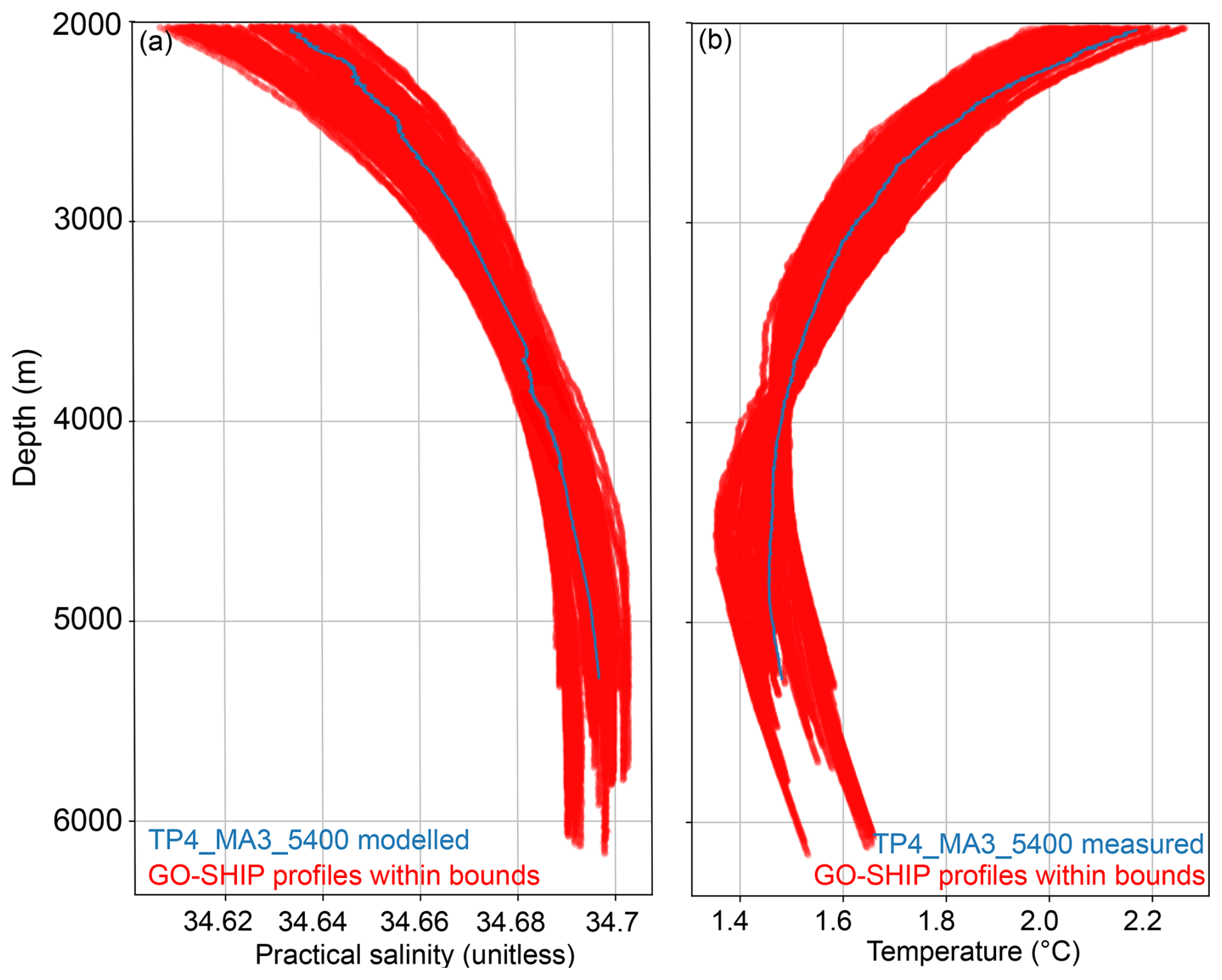
Figure A1 Profiles over 2000 m of TP4_MA3_5400 and GO-SHIP datasets for (a) modelled salinity (blue) compared to the measured GO-SHIP profiles (red) within the bounds and used for this GMM and (b) associated measured temperature (blue) and measured GO-SHIP profiles (red).

We applied Gaussian mixture modelling to achieve a modelled representation of the practical salinity (SP) from 2500 m to the seafloor at each voyage deployment location (Table A1). Such unsupervised classifications have been completed for CTD profiles and Argo floats (Ye and Zhou, 2025; Zhang et al., 2023). All GO-SHIP profiles deeper than 5000 m and within 10° latitude and 10° longitude from the voyage site were used in scikit-learn package GaussianMixture (GMM) (Pedregosa et al., 2011). If there were 2 or less GO-SHIP profiles within the bounding box, it was expanded to 15° latitude and 15° longitude, otherwise the site was excluded. Mixture models can be viewed as an extension of k-means clustering that integrates information regarding the covariance structure of the data alongside the centres of the latent Gaussian distributions. They are a probabilistic framework that assumes all data points are derived from a combination of a finite set of Gaussian distributions with unspecified parameters. Options within the package that were altered to get the optimal GMM model of SP were:

• covariance_type: tied or full, default is full.

• N_components: 1–21, number of mixture components.

• random_state: 42, controls the generation of random samples.

The rest of the parameters were kept as default values. Each set of GO-SHIP data for the associated TPT voyage site was iterated through each covariance type for each number of components. The elbow method was then used to choose the number of components, whereby the increase in the number of components does not equate to an increase in the model performance ($\text{AIC}/\text{BIC}$). An example modelled SP profile over depth and associated t, in-situ temperature profiles are shown for TP4_MA3_5400 in Fig. A1. The modelled seafloor salinity was then compared with a seafloor Niskin bottle salinity measurement at each site to provide a second validation of the profile. The water sample was analysed on the vessel using an 8400B Autosal Salinometer.

Table A1 Station metadata and gaussian mixture model details for each location.

Appendix B: Sensitivity analysis for threshold value (TH method) and ε value (DP method)

We used the collected profiles of temperature and pressure to test the optimal threshold value to use for the BML thickness derivation. We used the Quality Index methodology (Eq. 1 in the main text) to choose the appropriate threshold value based on Lorbacher et al. (2006) as it was being applied to the same method. The conservative temperature of 0.003 °C provided the highest mean QI for both the TPT voyage dataset and the GO-SHIP repeat hydrographic sections of P02 and P16 (Fig. B1).

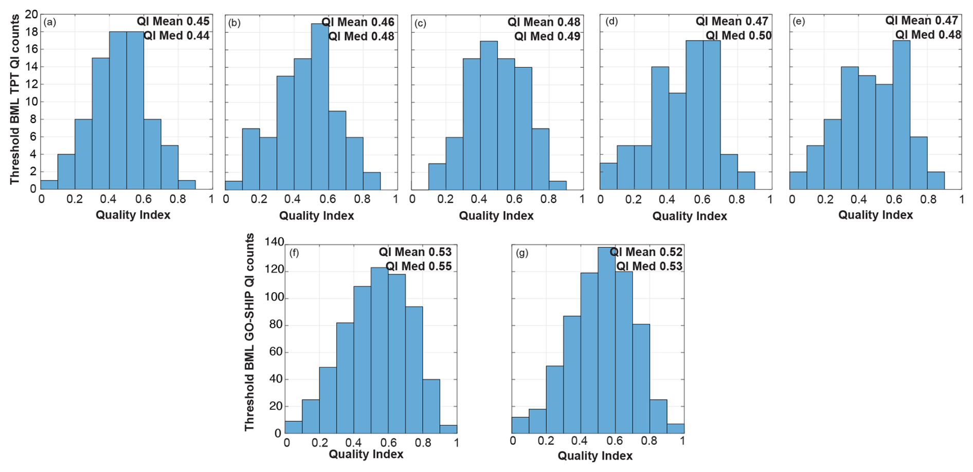
Figure B1 Histogram plots of the quality index values from the threshold BML height based on different threshold values of conservative temperature (Θ) for TPT profiles as (a) 0.001 °C, (b) 0.002 °C, (c) 0.003 °C, (d) 0.004 °C and (e) 0.005 °C and for the GO-SHIP profiles as (f) 0.003 °C and (g) 0.005 °C.

The Douglas–Peucker split-and-merge algorithm (Ahmadzadeh, 2017) reduces the number of points in a curve, approximating it by a series of points. An ε value between 0 and 1 is required to specify the similarity between the curve and the points, i.e. the smaller the epsilon, the more similar the curve. We tested three TPT Expedition profiles with ε values between 0.001 and 0.01 (Fig. B2 for site TP2_OM3_5400). We chose ε=0.002 and ε=0.008 as the two options with the most variability in results to calculate the BML height. This gave us methods DP02 and DP08 respectively.

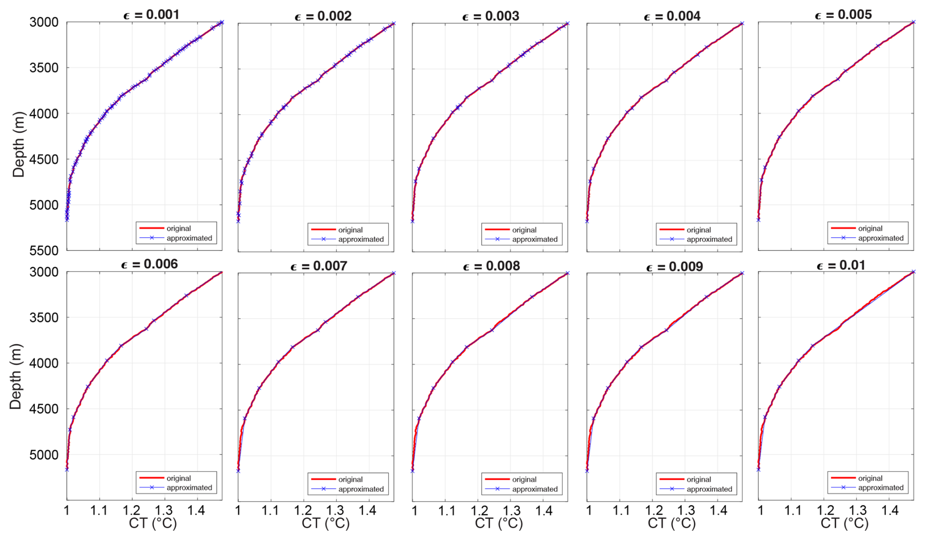
Figure B2 Douglas–Peuker Algorithm output (approximated, in blue) for different values of ε and original profile of TP2_OM3_5400 in red as an example.

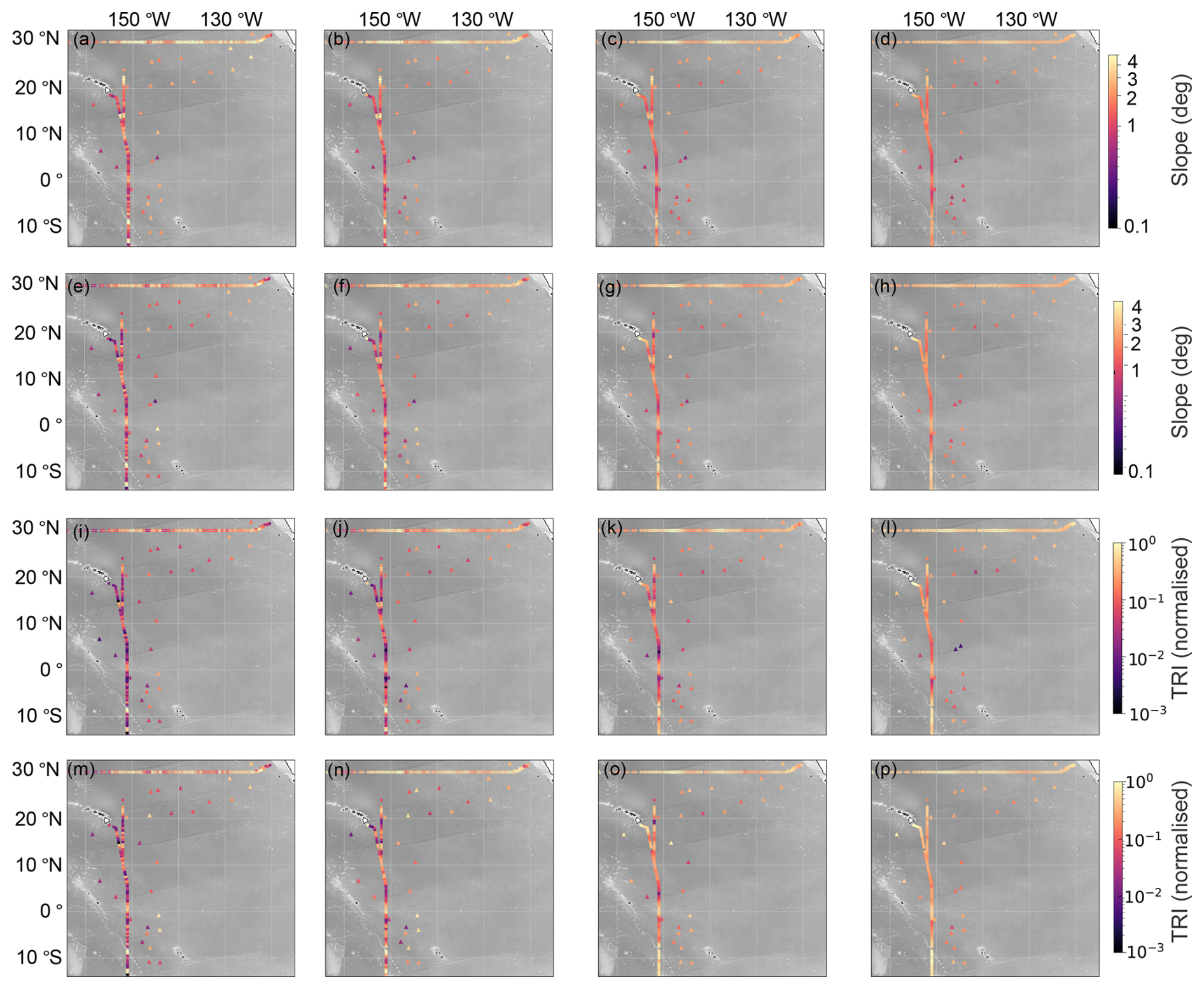
Figure B3 GO-SHIP (circle) and TPT (triangle) site variables of the (a–d) mean slope over 25, 50, 100 and 200 km buffer zones respectively (deg) and the (e–h) standard deviation of slope over the 25, 50, 100 and 200 km buffer zones respectively, (i–l) the mean normalised terrain roughness index (TRI) over the 25, 50, 100 and 200 km buffer zones respectively and (m–p) displaying the normalised standard deviation of the TRI. For the multiple TPT sites within close proximity (3 km), TRI and slope are on the centre point. The background regional bathymetry is from the Global Multi-Resolution Topography (GMRT) Synthesis Released CC BY 4.0 Deep | Attribution 4.0 International | Creative Commons Ryan et al. (2009).