The answer is blowing in the wind: seasonal hydrography and mixing of the inner sea of Tierra del Fuego, Southern Patagonia

This study characterizes seasonal hydrography and mixing processes in Almirantazgo Fjord, a sensitive ecosystem in southern Chilean Patagonia. Although estuarine and tidal forcing conventionally explain fjord dynamics, wind stress effects remain less understood in this high-latitude region. The study analyses a comprehensive six-month dataset including a moored time-series of temperature, salinity, and dissolved oxygen, cross-fjord CTD transects, and hydrographic profiles derived from seal-deployed sensors. Observations indicate distinct seasonality, shifting from a stratified water column in summer – defined by low-salinity surface water from glacial melt – to a mixed winter state with significantly reduced vertical stability. The analysis identifies persistent, topographically channelled up-fjord winds as a primary physical driver. By applying the Wedderburn number (Wb) and mechanical energy balance calculations, we determined that strong wind stress perturbs the pycnocline (Wb > 1). During stratified summer periods, strong wind events (above the 90th percentile) generated wind power of the same order of magnitude as that of the estuarine circulation. Under such conditions, wind forcing amplifies vertical mixing, modulates the pressure gradient, and supports oxygenation in the upper and subsurface layers. First-order estimates indicate that the upper brackish layer is flushed in approximately one week, reflecting a dynamic surface exchange governed by the interplay of freshwater buoyancy and wind stress. These results indicate that wind constitutes a primary mechanism regulating the hydrographic structure and biogeochemical function of the Tierra del Fuego inner sea.

1 Introduction

Fjord basins originate from glacial advance and retreat, processes that produce elongated narrow basins characteristically containing one or several glacial moraines known as sills (Dyer, 2019; Farmer and Freeland, 1983; Geyer and MacCready, 2014; Inall and Gillibrand, 2010; Stigebrandt, 2012). These ecosystems play a key role in CO₂ sequestration, a function resulting from the undersaturation of their surface waters (Aalto et al., 2021). Furthermore, the growing utilization and exposure of these systems has led to their designation as “aquatic critical zones” (Bianchi et al., 2020).

In these coastal systems, numerous processes operate on different temporal and spatial scales. This results in a complex combination of forces that determines the observed circulation patterns in regional and small-scale basins. Typically, residual circulation in shallow water estuaries had been described as two-layered and density driven (Officer, 1976; Valle-Levinson et al., 2014). The density differences produce an along-fjord pressure gradient, due to freshwater input at the fjord head and authors like Officer (1976), Dyer (1997) and Valle-Levinson et al. (2014), attributed as the main drivers of residual circulation. This gradient produces the two-layered, along-fjord gravitational circulation (Hansen and Rattray, 1965; Ribeiro et al., 2004). This pattern is manifested as a residual circulation pattern after several tidal cycles (MacCready and Banas, 2012) and can be substantially modified by wind stress (Guo and Valle-Levinson, 2008), bathymetric and frictional effects, the Earth's rotation (Yang et al., 2015), and drag (McCabe et al., 2006).

In deep-waters estuaries, like fjords, the two-layer circulation is often confined to a narrow portion of the water column, sequestered within a sharp pycnocline (Valle-Levinson et al., 2014). This fundamental structure is subject to modification by several external forcings, including wind stress (e.g., Klinck et al., 1981; Castillo et al., 2017), remote density gradients (Stigebrandt, 2012), and tidal action (Ianniello, 1977; Valle-Levinson et al., 2007). Observations in Chilean fjords, particularly in northern Patagonia, have identified three-layer residual circulation patterns. Although these are primarily attributed to tidal forcing in deep fjords, the signal is relatively weak and often obscured by wind-driven effects (Valle-Levinson et al., 2014). Furthermore, research in Douglas Channel, British Columbia demonstrates a seasonal shift from three-layer circulation in summer to a four-layer structure in winter. Such transitions are likely driven by the dynamic adjustment of estuarine flow, direct wind forcing, and the coupled barotropic and baroclinic responses to fluctuations in surface wind stress (Wan et al., 2017).

A complete description of fjord circulation must consider the cross-fjord dynamics. This cross-fjord pattern is generally weak and consists of an overturning motion known as secondary circulation (Chant, 2002; Lacy and Monismith, 2001; MacCready and Geyer, 2010). The along-fjord wind stress can intensify the estuarine circulation during down-fjord winds or weaken the surface outflow during up-fjord winds (e.g. Valle-Levinson, 2010). The study of Jackson et al. (2025) shows that strong winds and weak stratification facilitate mixing of the water column promoting deep ventilation. In some fjords katabatic winter winds can lead cooling and reoxygenate subsurface waters for longer time like in Blue Inlet, British Columbia (Bianucci et al., 2024). This type of wind interaction, down-fjord winds, can drive upwelling that exposure deep water to the air-sea interface (Klymak et al., 2025).

Chilean Patagonia is one of the most extensive fjord regions of the world; the shape of this region was formed by the combined effect of glacial erosion since the Quaternary and the tectonic sinking of the central valley (Aracena et al., 2011). The region is formed by more than 100 000 km of coastline and 40 000 thousand islands, which generate a complex system of fjords and channels as unique marine ecological hot spots (Hucke-Gaete et al., 2023; Landaeta et al., 2023). This system of channels and fjords in Chile between 41 and 56° S has been geographically classified into three zones: the northern (41–46° S), the intermediate (46–50° S), and the southern (53–56° S) Patagonia (Pickard and Stanton, 1980). Early studies of the Chilean fjords indicated strong parallels with British Columbia fjords (Pickard, 1971; Farmer and Freeland, 1983).

Observations from the last four decades indicate that the predominant zonal (east-west) winds in Southern Patagonia have strengthened at a rate of 0.2–0.3 m s⁻¹ per decade (Garreaud et al., 2013; Giesecke et al., 2021). This strengthening is consistent with an increase in rainfall at a rate of 200 mm per decade in areas south of latitude 50° S (Garreaud et al., 2013). In the region, the Southern Annular Mode (SAM) is related with the generation of the westerlies (Aguayo et al., 2019). The SAM drives the formation of regional westerlies and has shifted toward its positive phase in response to climate change (Garreaud et al., 2013; Aguayo et al., 2019). This positive phase has been connected to an increase to 30 % of the westerly winds since 1950 (Downes et al., 2017). El Niño-Southern Oscillation (ENSO) is another significant interannual climate pattern. During El Niño events, a reduction in freshwater inflow is associated with greater vertical mixing and the advection of oceanic waters into northern Patagonia's fjord systems (León-Munõz et al., 2018).

The global increase in temperature (IPCC, 2023) suggests a significant alteration in the global heat budget and affects the retreat of ice sheets and mountain glaciers (Church et al., 2013). Interaction between glaciers and atmosphere can generate a local wind circulation known as katabatic winds (Spall et al., 2017; Bianucci et al., 2024). These winds are a common characteristic of fjords adjacent to glaciers where they can exceed 20 m s⁻¹ (Farmer and Freeland, 1983; Stigebrandt, 2012; Spall et al., 2017). Along-channels winds may also advect heat and modulate the supply of warmer waters, thereby promoting glacial retreat (Moffat, 2014). The loss of glacial fields in southern Patagonia has been estimated at 10 % (Rivera et al., 2017). In addition, within this framework, accelerated glacial melting and the subsequent freshening of surface waters directly impact vertical stratification (e.g. Boone et al., 2018). These alterations in freshwater input, combined with shifts in wind-stress intensity (which modulates mixing), could substantially modify the dynamics of sub-polar systems such as the Strait of Magellan and the inner sea of Tierra del Fuego. The southern Patagonia has two major ice-field glacial: the northern and the southern ice-field (Garcés-Vargas et al., 2026), a smaller glacial formation is located at the study region the Darwin Cordillera (Fig. 1). In these regions, katabatic flow plays an important role in defining on-glacier temperatures for valley glacier (Bravo et al., 2019). Thus, the increase of glacial melting could diminish the glacial area impacting in the katabatic flow intensity.

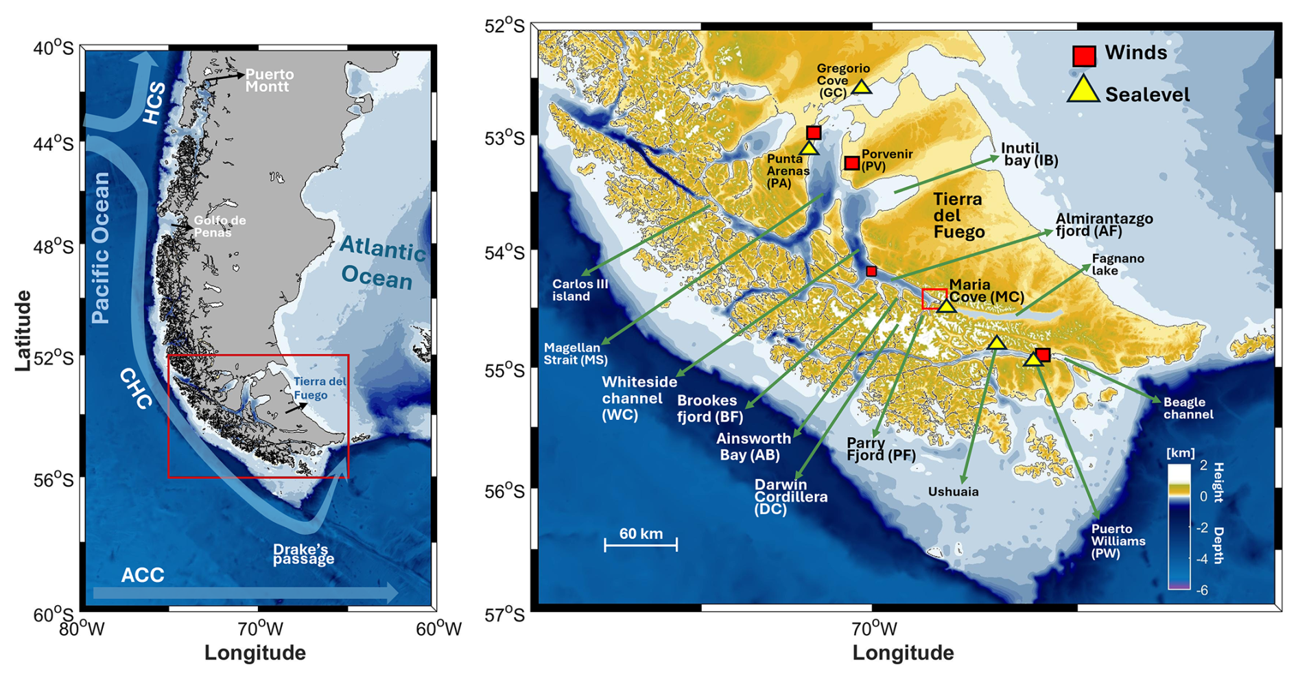
Figure 1 Study region. At the left side, a regional map of the interest region shows the main currents systems: the Humboldt Current System (HCS), the Cape Horn Current (CHC) and the Antarctic Circumpolar Current (ACC). At the right, the complexity of the Southern Patagonia it is shown, here bathymetry and topography are sowed in colorscale. Geographic features referenced in the text are identified, including Magellan Strait (MS), Inutil Bay (IB), Whiteside Channel (WC), Almirantazgo Fjord (AF), Brookes Fjord (BF), Ainsworth Bay (AB), Parry Fjord (PF), and Maria Cove (MC). The Darwin Cordillera is denoted by white-shaded high-altitude areas on the island of Tierra del Fuego. Depths and highs data were downloaded from © GEBCO Compilation Group (2025).

While the effects of density and tidal driven circulation on estuarine dynamics are well-documented (e.g. Farmer and Freeland, 1983; Stigebrandt, 2012; Geyer and MacCready, 2014), wind-driven circulation has received comparatively less attention (Soto-Riquelme et al., 2023). Investigations of wind-driven circulation and its effects on the inner-sea of the Chilean Patagonia have been conducted in specific systems within northern and central Patagonia. These include the Reloncaví fjord (e.g. Valle-Levinson et al., 2007; Castillo et al., 2012, 2017), the Reloncaví sound (Letelier et al., 2011), the inner-sea of Chiloe (Soto-Riquelme et al., 2023; Linford et al., 2024), the Guafo mouth (Ross et al., 2025), the Moraleda channel (Valle-Levinson and Blanco, 2004), the Aysen fjord (Cáceres et al., 2002) and Jorge Montt Glacier (Moffat, 2014). Regional Patagonian wind patterns were analysed by Pérez-Santos et al. (2019). At this spatial scale, atmospheric rivers have been identified as important factors controlling the regional wind effects (Garcia-Santos et al., 2025). However, although this region is characterized by intense winds and strong tidal modulation (Antezana, 1999; Garreaud et al., 2013; Brun et al., 2020), the effects of the wind on the physical dynamics of the inner-sea of Tierra del Fuego remain poorly understood.

The intermediate zone (46–50° S) receives significant freshwater input within the Penas Gulf, originating principally from glacial discharge. Here, glacier is the primary source, and this freshwater contribution has been reinforced in recent years. The resulting freshwater interacts with the Cape Horn Current (CHC), causing its advection out of the Gulf. While the magnitude of these salinity anomalies decreases, they remain detectable, extending south of 50° S and north of 46° S (Cisternas et al., 2026).

The Southern Patagonian region is strongly affected by the Cape Horn Current (CHC), which is recognized as a component of the Antarctic Circumpolar Current (ACC) system (Lamy et al., 2015; Wu et al., 2019). Nevertheless, knowledge of the CHC's strength and variability remains limited (Zheng et al., 2023). Observational studies report current velocities exceeding 15 cm s⁻¹ (Chaigneau and Pizarro, 2005), while nearshore measurements show velocities greater than 30 cm s⁻¹ (Giesecke et al., 2021). Furthermore, an analysis combining model output and altimetry data calculated a CHC transport of 4.36 Sv. This value is comparable to the transport of the Humboldt Current System (HCS) between 5° S (1.8 Sv) and 15° S (5.2 Sv) (Chaigneau et al., 2013). More recently, research combining model output and in-situ observational data indicates that the CHC is largely geostrophic south of 49° S. This work also shows no clear seasonal variability with velocities of up to 0.3 m s⁻¹ in the upper 200 m of the water column (Garcés-Vargas et al., 2026).

This study investigates the hydrographic response of the Almirantazgo Fjord – one of the southernmost fjords of South America, in Tierra del Fuego, Chilean Patagonia – to freshwater input from glacial melting and to along-fjord wind-stress. To describe the variability of the water column and its response to wind forcing, a six-month dataset was analysed. This dataset combines a time series of salinity, temperature, and dissolved oxygen with in-situ hydrographic data acquired from fixed CTD stations and animal-borne satellite CTD.

2 Material and methods

2.1 Study region

The Magellan Strait, situated in the southern Patagonia fjord region, connects the Atlantic and the Pacific oceans. Its internal dynamics govern the hydrography of the surrounding inland sea. Despite a sparse population, southern Patagonia possesses considerable economic significance for Chile. The growth of industries such as aquaculture, oil, green hydrogen, and tourism has altered land use, transport, and increased the ecological pressure on the Magellan Strait, Tierra del Fuego, and the Beagle Channel (Ariztía and Undurraga, 2025; Giesecke et al., 2024).

Large freshwater inputs from riverine and glacial sources significantly affect the region (Sassi and Palma, 2006). The low salinity of the Magellan Strait results from a north-eastward flow from the Patagonian Current (Brun et al., 2020). The distribution of these waters is governed by the combined effects of wind, tides, and the Antarctic Circumpolar Current (Palma and Matano, 2012). Previous research indicates that waters from the Atlantic Ocean extend their effect westward through the Magellan Strait as far as Punta Arenas. In contrast, the effect of the Pacific Ocean extends eastward to Carlos III Island, where a shallow sill limits its influence on surface waters (Antezana, 1999; Brun et al., 2020).

An important geographical feature is the Darwin Cordillera (DC) mountain range which extends 200 km from west to east along the southwestern peninsula of Tierra del Fuego Island (Fig. 1). The DC is the core of the southern westerlies and experiences low precipitation. The region is characterized by a strong W–E temperature gradient (Carrasco et al., 2002; Garreaud et al., 2013; Meier et al., 2018; Izagirre et al., 2024). Near the study region (Fig. 1c), the glaciers of Parry fjord have been relatively stable since 1986, but the Darwin glacier retreated 3 km between 1986 and 2014. In this period, the region's glaciers have lost 10 % of their area (Rivera et al., 2017).

The Almirantazgo Fjord (AF) is 75 km long, with a width of 16 km in the northern part and 5 km near its head with an averaged width of 12 km. The AF axis is 116° from the true north, an approximately East-Southeast (ESE) direction. It contains three major glacial connections: Brookes fjord (BF), the Ainsworth bay (AB), and Parry fjord (PF). At the head of the fjord, in Maria Cove, the fjord is shallow, with a mean depth of approximately 30 m for the first 7 km. The bottom then slopes steeply until the mouth of PF, deepening from 30 to 200 m in less than 3 km. From PF to BF, the fjord depth is approximately 220 m. The deepest part of this basin is in the Whiteside channel (WC), where the bottom depth is approximately 450 m. This is one of the deepest parts of the inner sea of Tierra del Fuego (Fig. 1).

2.2 Atmospheric data

Meteorological data for the region were obtained from the Dirección General de Aeronáutica Civil (https://climatologia.meteochile.gob.cl/, last access: 16 June 2026), sourced from airports at Punta Arenas (53.00° S, 70.84° W), Porvenir (53.25° S, 70.33° W), and Puerto Williams (54.93° S, 67.62° W). The dataset included wind magnitude and direction (meteorological convention), recorded at 1 h time intervals between 1960 and 2025.

Additionally, to characterize the wind patterns, this study uses wind reanalysis data from ERA 5. The wind components at 10 m high (u₁₀, v₁₀) were downloaded in spatial grids of 0.25° × 0.25°. The ERA5 is the fifth-generation ECMWF reanalysis of global climate and weather data. Reanalysis integrates model data worldwide observations into a globally complete and consistent dataset on physical laws (Hersbach et al., 2023).

Wind-stress (τ) was calculated using the bulk formula by $\mathit{\tau }=r_{\mathrm{a}}{c}_{\mathrm{d}}\left|U_{\mathrm{10}}\right|{\mathit{U}}_{\mathrm{10}}$, where r_a is the air density (1.2 kg m⁻³), U₁₀ is the wind velocity vector (with components u₁₀, v₁₀), $\left|U_{\mathrm{10}}\right|$ is wind speed (the scalar magnitude of U₁₀) and c_d is dimensionless wind-drag coefficient. The coefficient c_d was calculated for each wind component value in the time-series following Yelland and Taylor (1996), for $\left|U_{\mathrm{10}}\right|<\mathrm{6}$ m s⁻¹, $c_{\mathrm{d}}=(\mathrm{0.29}+\mathrm{3.1}|U_{\mathrm{10}}{|}^{-\mathrm{1}}+\mathrm{7.7}\left|U_{\mathrm{10}}{|}^{-\mathrm{2}}\right)\times {\mathrm{10}}^{-\mathrm{3}}$, whereas, for 6 m s⁻¹ ≤ $\left|U_{\mathrm{10}}\right|$ ≤ 26 m s⁻¹, $c_{\mathrm{d}}=(\mathrm{0.60}+\mathrm{0.07}{U}_{\mathrm{10}})\times {\mathrm{10}}^{-\mathrm{3}}$.

2.3 Sea Level data and tides model

Sea level data were acquired from four tide gauge stations located within the inner sea of the Magellan Strait and the Almirantazgo Fjord (Fig. 1): Gregorio Cove, Punta Arenas, Puerto Williams, and Ushuaia (Table 1). The dataset was obtained from the Sea Level Station Monitoring Facility (https://www.ioc-sealevelmonitoring.org/, last access: 16 June 2026) for the period of January to June 2024. At each station, measurements are recorded at a one-minute interval by a pressure sensor positioned near the seabed.

Additionally, a barotropic tidal global model TPXO9 (Egbert and Erofeeva, 2002) was applied to determine the spatial distribution of amplitude and tidal current ellipses in the region (Fig. 3). The model provides complex tidal heights (h) and transport coefficients for 15 constituents at $\mathrm{1}/\mathrm{30}$° resolution. The principal harmonic amplitudes (M₂, N₂, S₂, O₁, and K₁) were used to estimate the form factor (e.g. Pan et al., 2024) defined as $F=(O_{\mathrm{1}}+K_{\mathrm{1}})/(M_{\mathrm{2}}+S_{\mathrm{2}})$ was useful to characterize the regimes of the barotropic tide in the inner sea of Tierra del Fuego.

2.4 Hydrography data

The hydrography data were obtained using two different complementary methods: conventional CTDOF (AML Metrec X) deployments and CTDF (CTD-SRLD) casts from sensors affixed to Southern elephant seals.

The conventional instrumentation consisted of a CTD AML–Metrec X equipped with Temperature, Conductivity, Pressure, Fluorescence/Chlorophyll, and pH sensors, supplemented by an additional Aanderaa Optode 4831 infrared Dissolved Oxygen sensor. The CTDOF was configured for freshwater settings to permit measurements under low-conductivity conditions, with profiles acquired at a rate of four scans per second. At each oceanographic station, the instrument was activated on deck and subsequently lowered to 1 m below the surface, where it was held for one minute to ensure sensor stabilization. Data acquisition was then performed using an electrical winch to a depth up 200 m. To describe the oceanographic conditions, sampling was conducted at five cross-fjord oceanographic stations (Fig. 1). Data were collected during the austral summer (15 and 31 January 2024) and the austral winter (26 and 30 June 2024). A total of 60 cross-fjord profiles were acquired to characterize the oceanographic conditions near the head of the Almirantazgo Fjord. Post-processing of the AML-CTD data followed standard quality control procedures, consistent with other CTD instruments. This process included: visual inspection to remove spikes, exclusion of sensor stabilization time, selection of downward profiles, and vertical binning at 0.5 m intervals. Subsequently, mean profiles for January and June were calculated for each station and are presented in Fig. 6.

Oceanographic conditions in the region were also assessed using CTD-SRLD (Boehme et al., 2009) and CTD-Fluoro tags (Guinet et al., 2013). The CTD tags possess high accuracy (±0.005 °C for temperature, ±0.01 mS cm⁻¹ for conductivity, and 2 dBar ± (0.3 + 0.035 % reading) K⁻¹ for depth) and were calibrated by the manufacturer prior to deployment. These tags were affixed to Southern elephant seals (Mirounga leonina) from the colony located at Jackson Bay, located at the head of the Almirantazgo Fjord (Fig. 1c). In-situ temperature and salinity measurements were converted to Absolute Salinity (S_A), Conservative Temperature (Θ) following the TEOS-10 (McDougall and Barker, 2011).

Water column stratification was characterized by the buoyancy frequency (N²), calculated as $N^{\mathrm{2}}=-g/{\mathit{\rho }}_{\mathrm{0}}\partial \mathit{\rho }/\partial z$, where g is the gravitational acceleration, ρ₀ is the reference density, and $\partial \mathit{\rho }/\partial z$ is the vertical density gradient. Additionally, CTD data were used to estimate the energy required to homogenize the water column, expressed as the Potential Energy Anomaly (PEA), $\mathrm{PEA}=\mathrm{1}/h{\int }_{-d}^{\mathrm{0}}gz({\mathit{\rho }}_p-\mathit{\rho })\mathrm{d}z$, where h is the thickness for the calculation of average density (ρ_p). A high PEA value corresponds to high stratification (Simpson et al., 1979). The Freshwater Content (FWC), defined as the equivalent thickness of freshwater in the water column, was also calculated, $\mathrm{FWC}={\int }_{-d}^{\mathrm{0}}(s_{\mathrm{0}}-s)/s_{\mathrm{0}}\mathrm{d}z$, where s₀ is the reference salinity at depth d (Blanton and Atkinson, 1983), here the study used s₀=31 g kg⁻¹ which was the maximum salinity in the deeper zone of the Almirantazgo fjord. In all the profiles FWC was calculated by integrating over the entire water column down to the bottom depth.

To describe the hydrographic along-fjord patterns for January and June 2024, this study utilizes CTD-SRDL data collected between Inútil Bay (IB) and María Cove (MC). Although the elephant seals provided numerous hydrographic profiles across the region, the study defined an along-fjord route along the central axis between IB and MC (see Fig. 5a). This route consisted of points spaced at 0.1 km intervals over a 150 km span. All profiles within 2 km of each point, in a temporal window of 3-weeks centred at the CTD-AML dates (see Table 1), on the route were selected and averaged to obtain a single representative profile per point. For the vertical dimension, standard depths were established at every 1 m (0–20 m), 5 m (20–50 m), 10 m (60–100 m), and 50 m (150–500 m). Vertical interpolation was performed only at these standard depths, avoiding spatial (distance) along-fjord interpolation. This procedure was applied to the January and June 2024 data shown in Fig. 5c, d.

To assess the influence of different water masses, an Absolute Salinity of 31 g kg⁻¹ was used as an index defining the upper boundary of the Modified Subantarctic Water (MSAAW). This water mass is produced by the combination of surface freshwaters with Subantarctic Water (SAAW), the dominant water mass within the region (Silva and Vargas, 2014).

2.5 Time series: observations and data analysis

Time series data of the water column properties were acquired using two distinct but complementary ways. The first method comprised a six-month (January–June 2024) near-bottom (30 m depth) record of sea level, salinity, temperature and dissolved oxygen. The second method involved short-term (5 d) acquisitions of a fine vertical-scale temperature, salinity and dissolved oxygen during January 2025 (Fig. 2).

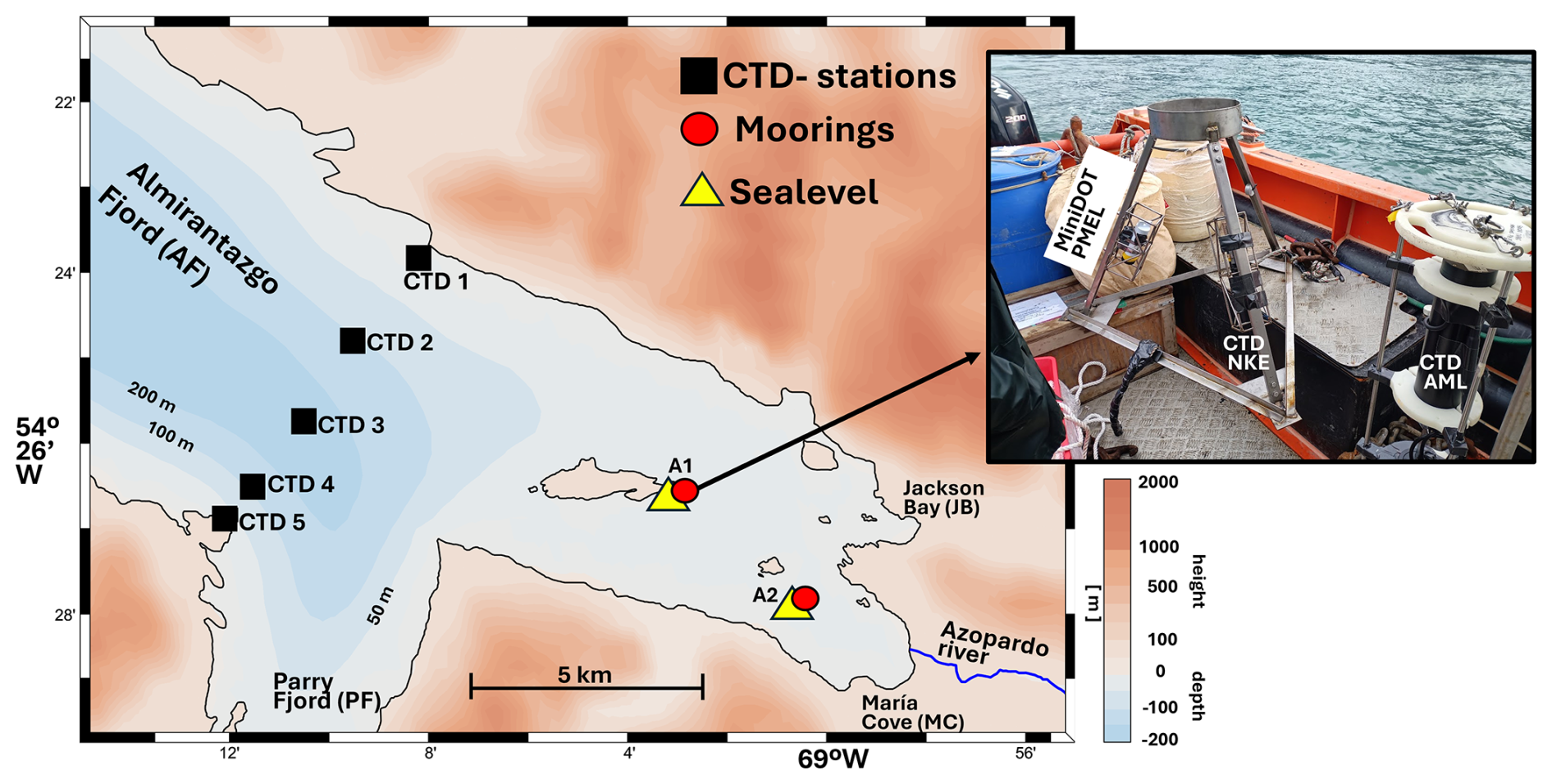
Figure 2 Location of the oceanographic stations at the head of the Almirantazgo fjord. The caption shows the location of oceanographic stations and mooring deployments within the innermost part of the Almirantazgo Fjord. In addition, the mooring system deployed at the sites and the instrumentation it is shown. Depths and highs data were downloaded from https://www.gebco.net/data-products/gridded-bathymetry-data (last access: 16 June 2026). Bathymetric data © GEBCO Compilation Group (2025).

The six-month time series was collected using a CTD WiSens NKE Instruments (https://nke-instrumentation.com/, last access: 16 June 2026). This instrument was secured within a stainless steel, pyramid-shaped frame (1 m × 1 m; 0.7 m height) positioned on the seabed at 30 m depth near to 54.44° S, 69.05° W. The instrument specifications include a pressure range up to 300 m (0.1 % accuracy), a temperature range of the −2 to 35 °C (±0.02 °C), and salinity range 2 to 42 PSU (±0.1 PSU). Dissolved oxygen (DO) concentration was recorded by a PMEL MiniDOT (https://www.pme.com/products/minidot, last access: 16 June 2026), which functions via an optical sensor. This sensor has an accuracy of ±0.2 mL L⁻¹ and a resolution of $\mathrm{7}\times {\mathrm{10}}^{-\mathrm{4}}$ mL L⁻¹. The MiniDOT also contains temperature sensors with a range of 0 and 35 °C ±0.1 °C and its housing is rated for 300 m depth. Both the Wisens NKE and MiniDOT sensors were affixed in individual stainless-steel frames attached to the main pyramid structure. This entire assembly was lowered to the bottom and remained moored until retrieval at the end of June 2024.

The 5 d time series was acquired from a mooring at A2 station (Fig. 2, Table 1) between 22 and 26 January 2025. This instrument array was designed to measure the vertical gradient of temperature, salinity, DO, and pressure. The array included CTD NKE WiSens and a miniDOT positioned at 0.3 m depth and at 30 m depth (near the bottom) to determine the vertical gradients of salinity ($\partial S/\partial z$), temperature ($\partial T/\partial z$), and dissolved Oxygen ($\partial \mathrm{DO}/\partial z$).

To characterize the temporal variability and dominant oscillations observed in the data, a Morlet wavelet analysis (Torrence and Compo, 1998; Grinsted et al., 2004) was applied to the time series of wind stress, sea level, Conservative Temperature, Absolute Salinity, and Dissolved Oxygen. This method permits the computations of both the dominant modes of variability and their temporal variations (Torrence and Compo, 1998). To quantify the relationship between the wind stress and the other variables, wavelet coherence was estimated following the methodology of Grinsted et al. (2004).

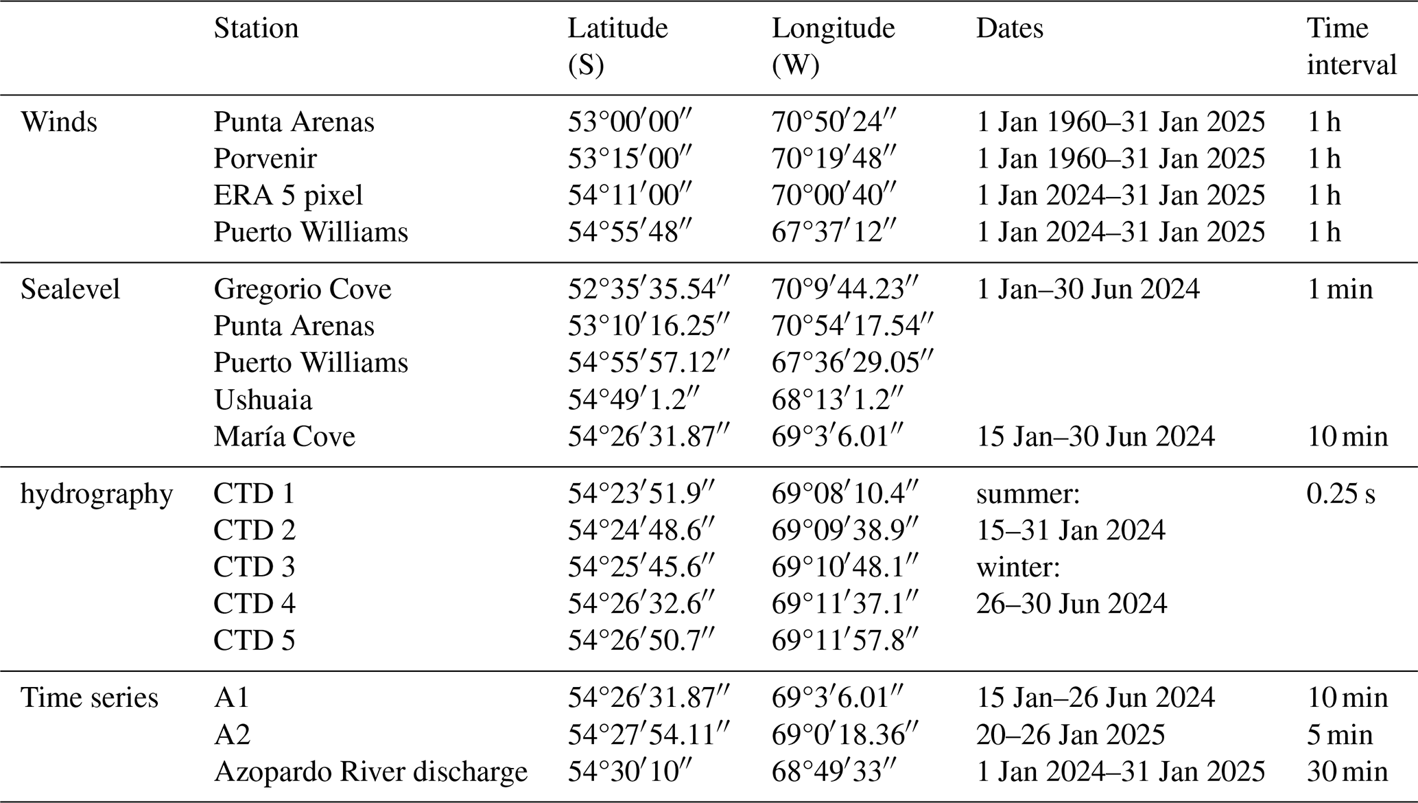
Table 1 Location and descriptions of the sea level stations, hydrographic (oceanographic) stations, and time series data used in the study.

The potential for the wind stress to perturb the pycnocline was assessed using the dimensionless Wedderburn number (Wb) following Geyer (1997), Thorpe (2005) and Inall et al. (2015). The number is defined as: Wb = $\left(\mathit{\tau }L\right)(\mathit{\rho }g{)}^{-\mathrm{1}}{h}_{\mathrm{1}}^{-\mathrm{2}}$, where L is the length of the fjord (or the horizontal scale of the wind), g is gravitational acceleration, and h₁ is the depth of the upper layer directly influenced by the wind stress τ. In a simplified two-layer model, the density difference $\mathit{\rho }={\mathit{\rho }}_{\mathrm{2}}-{\mathit{\rho }}_{\mathrm{1}}$ where ρ₁ and ρ₂ are the densities of the upper and deeper layer, respectively. According to this formulation, a value of Wb < 1 indicates that the density gradient dominates. When Wb = 1, wind forcing and buoyancy effects are comparable, and horizontal mixing becomes significant When Wb > 1, wind-driven effects are dominant (Inall et al., 2015).

3 Results

3.1 Wind pattern: seasonality of the zonal and meridional components

The 54-years hourly reanalysis dataset was used to establish the wind climatology for the study region (Fig. 2). The results indicate that seasonal winds exhibit high directional consistency. Westerlies are the dominant pattern; south of 54° S in the Pacific Ocean, these winds acquire a slight southerly component, with the airflow generally following the coast. Wind magnitudes intensify near the coast, particularly during the warmer seasons (austral spring and summer), when speed exceeds 8 m s⁻¹ (Fig. 2a, b). During the colder seasons (austral autumn and winter), regional winds are weaker (<6 m s⁻¹), particularly offshore in the Pacific Ocean. Within the inner sea of the Magellan Strait and Almirantazgo Fjord, wind magnitude was low (<4 m s⁻¹), comparable to those observed in the open ocean. Regarding direction, winds within the Almirantazgo Fjord appear aligned with the fjord's axis and generally flow toward the fjord head throughout all the seasons (Fig. 2).

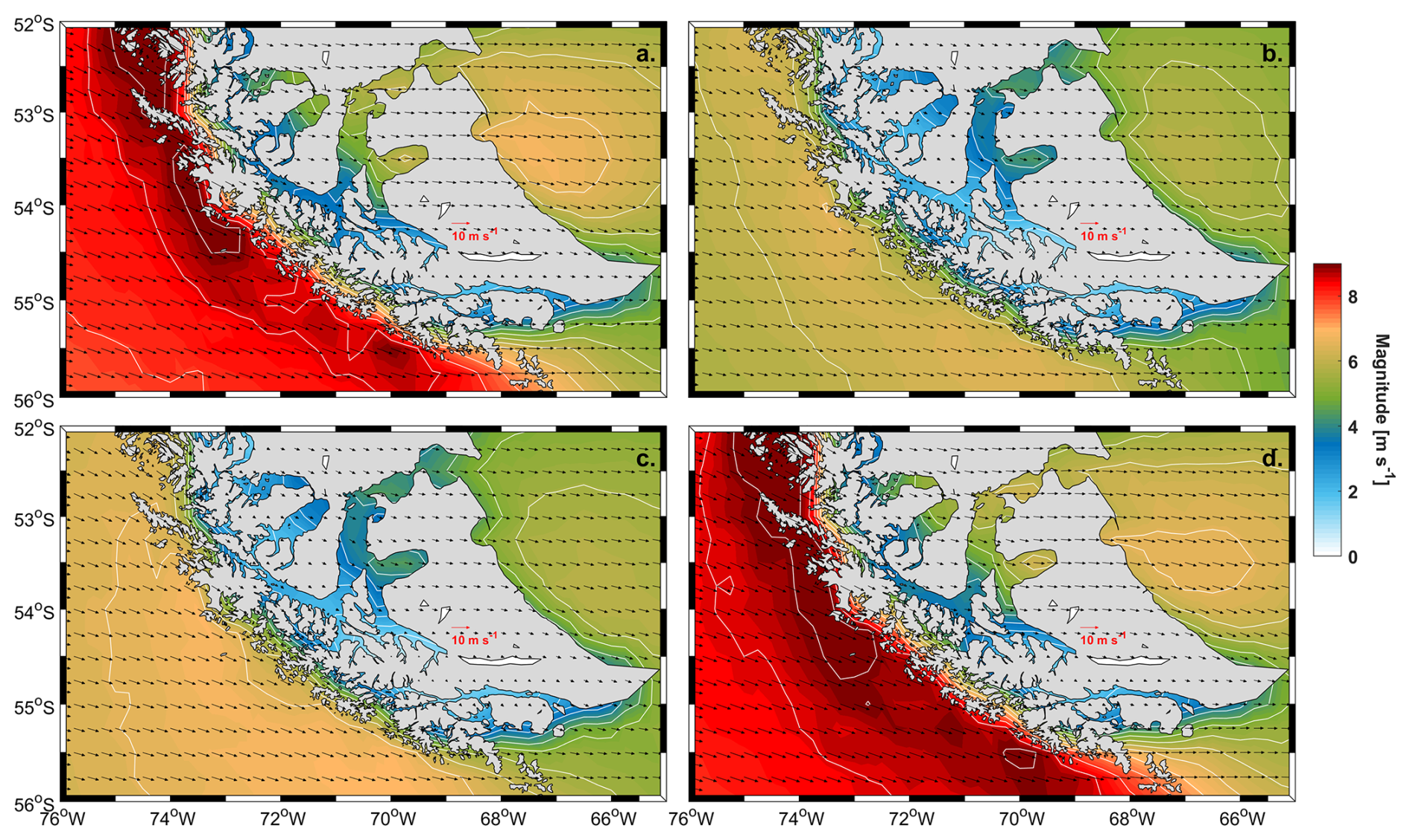
Figure 3 Climatology of winds in southern Patagonia. Mean wind vector are shown for the periods: (a) JFM (January–March, austral summer), (b) AMJ (April–May, austral autumn), (c) JAS (June–September, austral winter), and (d) OND (October–December, austral spring). Data were derived from hourly 0.25 × 0.25° gridded ERA5 reanalysis data covering the period 1970–2024. ERA5 reanalysis data © ECMWF/Copernicus.

The climatology from the meteorological stations indicates a high consistency with the regional winds described previously (see Fig. A1 in the Appendix). At Punta Arenas (PA), Porvenir (PV) and Puerto Williams (PW), eastward winds (meteorological westerlies) were predominant (>25 %) during all the seasons. The highest wind speeds (ca. 15 m s⁻¹) were observed at PA and PV during summer and spring. PV was an exception, as northward/southward winds were also recorded there during autumn and winter. For the Almirantazgo Fjord (AF) wind data were derived from a time series of an ERA5 reanalysis pixel (Fig. 3). At this location, the distribution of magnitude and direction was highly consistent with the regional patterns, showing a dominance of eastward winds in all the seasons. The directional distribution indicates that up-fjord winds (directed towards the fjord's head) are prevailing conditions in AF (see Fig. A1).

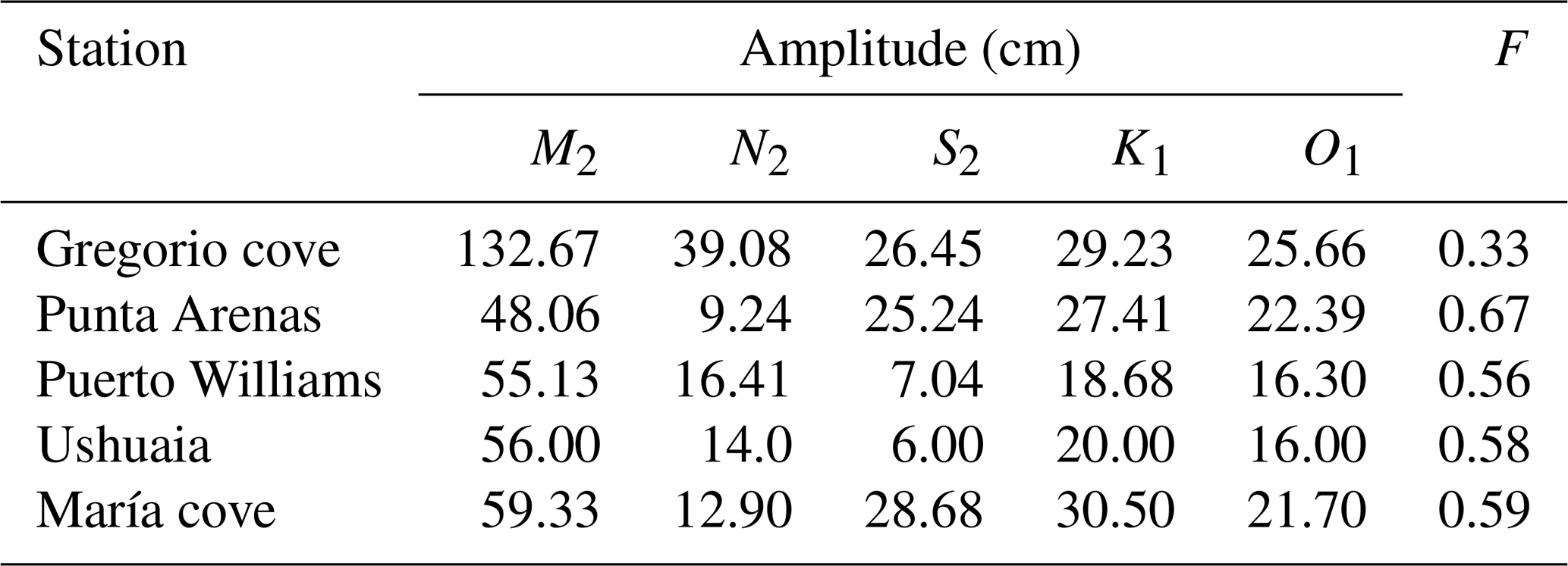
Table 2 Main tidal harmonics amplitude and form parameter (F) in the sealevel stations of the study region.

3.2 Sea level and Tidal influence on the region

Tidal amplitudes recorded by the region's tide gauges (Fig. 1, Table 2) were primarily controlled by the M₂ semi-diurnal harmonics. The Gregorio station measured an M₂ amplitude of 132.7 cm, a magnitude at least double that observed at the other stations (which ranged from 48 to 56 cm) located south of the Magellan Strait. At the Punta Arenas station, the M₂ amplitude was 48.1 cm. In the Beagle Channel, south of the Almirantazgo Fjord, the Puerto Williams and Ushuaia stations recorded comparable M₂ amplitudes of approximately 55 cm. The lowest F value (0.33) was observed at Gregorio, whereas at the other stations, F>0.6. The form factor (F) indicated that all the stations are characterized by a mixed, mainly semi-diurnal tidal regime.

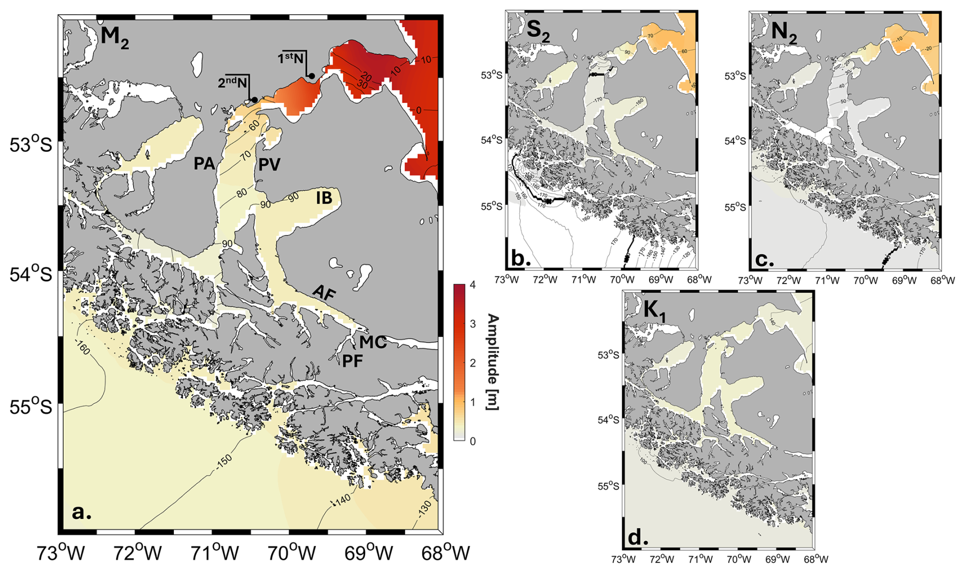
Figure 4 Results based on the tidal model by Egbert and Erofeeva (2002) shown the regional distribution of the principal harmonic constituents: (a) M₂, (b) N₂, (c) S₂, and (d) K₁. Amplitude (m) is represented by color shading, while phase (°) is shown as contour lines. In the caption, the locations of the First (1stN) and the Second Narrows (2ndN) within Magellan Strait are indicated. Tidal model data © Oregon State University (TPXO9; Egbert and Erofeeva, 2002).

To quantify the tidal influence in the study region, the barotropic tidal Model by Egbert and Erofeeva (2002) indicated that the northern part of the Magellan Strait and its connection with the Atlantic Ocean showed the highest M₂ amplitude (>3 m). Amplitudes decreased southward, falling below 1 m off Punta Arenas and reaching approximately 0.5 m inside the Almirantazgo Fjord (Fig. 3). A marked change in amplitude (from high to lower) was observed at the Second Narrow, phase tends to increase from the Atlantic (10°) to the inner-sea reaching 90° into the Inutil Bay. The entire basin from the Inutil Bay to Maria Cove seems to be in phase at 90°. Other harmonic constituents were substantially smaller than M₂ accounting for <10 % of the variability explained by the M₂ component (Fig. 4).

3.3 Temperature and Salinity patterns inside the Almirantazgo Fjord

The whole CTD-SRLD dataset (showed in Fig. A2) acquired from Southern elephant seals encompassed extensive areas, including the Pacific and Atlantic oceans and the inner sea of the Magellan Strait and Tierra del Fuego. To specifically address the dynamics of the Almirantazgo Fjord, the present analysis utilized only the CTD-SRLD data obtained from within the fjord. The hydrographic data reveal two distinct regimes for the waters of southern Patagonia (see Fig. A1d). Within the inner channels of Tierra del Fuego, low absolute salinity (ca. 31 g kg⁻¹) was observed in deeper waters (depths >100 m). Conversely, waters in the outer channels (in the Pacific and Atlantic oceans) were characterized by salinities exceeding 34 g kg⁻¹. These findings indicate that the inner channel waters are more stable (stratified) compared to the mixed conditions prevailing in the outer channels.

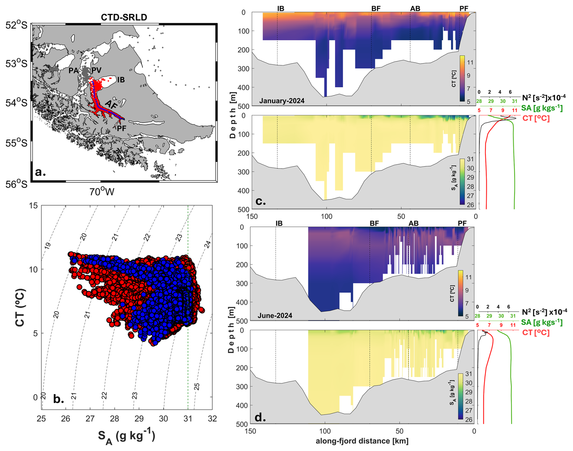
Figure 5 (a) Locations of the hydrographic profiles of Absolute Salinity (S_A) and Conservative Temperature (CT) acquired via CTD-SRLD (Southern elephant seals) and CTD-AML. CTD-SRLD data points within Bahia Inutil, Whiteside Channel, and Almirantazgo Fjord are marked in red. (b) CT/SA diagram the complete dataset (red dots) whereas in blue dots are the January and June elephants seals data showed in (c) and (d). Segmented black lines are isopycnals of conservative density anomaly (σ_CT) in kg m⁻³. (c) January and (d) June vertical sections of CT and SA for each month. The along-fjord blue dots in (a) indicates the along-fjord transect. Average profiles of Brunt-Väisälä frequency (N²), S_A, and CT for the entire transect are displayed to the right of the lower panels (c) and (d).

To compare and describe the seasonal patterns of the Almirantazgo Fjord, this study utilized CTD-SRLD data acquired from Southern elephant between January and June of 2024. The analysis was restricted to Conservative and Absolute Salinity measurements collected within the region extending from the Whiteside channel and Almirantazgo Fjord (Fig. 5).

The Conservative Temperature/Absolute Salinity (CT/S_A) diagram (Fig. 5) acquired by elephant seals, illustrates the wide hydrographic variability within Almirantazgo Fjord. S_A ranged from a minimum of 26.28 g kg⁻¹ near the surface (4 m depth) to a maximum of 31.13 g kg⁻¹ near the fjord bottom. CT varied from 4.24 to 10.94° C with a mean of 7.20±1.12 °C. The conservative density anomaly (segmented lines, Fig. 4b) extended from 1020.0 kg m⁻³ in the surface waters during January to a maximum of 1024.5 kg m⁻³ in near-bottom waters during June. The mean CT and S_A profiles (Fig. 5c, d) show pronounced upper-water-column stratification in summer, contrasting with the well-mixed conditions observed in winter.

The cross-fjord transect data were acquired using a CTD-AML Metrec during field measurements in January and July 2024. During the austral summer, S_A ranged from a minimum of 26.30 g kg⁻¹ near the surface to a maximum of 30.99 g kg⁻¹ near the bottom, with a seasonal average of 30.21±0.10 g kg⁻¹. Water temperature varies between 6.132 and 10.81 °C, with a mean of 7.68±0.03 °C.

During winter (June 2024), conditions in the Almirantazgo Fjord (AF) shifted. S_A ranged from 29.01 to 31.01 g kg⁻¹ with a mean of 30.78±0.04 g kg⁻¹. The water column was colder, with CT between 2.97 and 7.74 °C (mean: 7.01±0.06 °C). A thermal inversion was observed, with colder upper waters overlying warmer deeper waters. Density range was 1018.8 to 1024.5 kg m⁻³. Mean cross-fjord profiles indicated that stratification was salinity-dominated. In summer, continuously stratified conditions were present in the upper 30 m depth layer. In winter, however, the S_A profile was nearly homogeneous throughout the upper 100 m of the water column.

Based on the along-fjord and cross-fjord CTD sections and mean profiles (Figs. 5c, d and 6c, d), the study determined that during January, the thickness of the upper brackish layer near the head of the fjord (at PF) was h₁=20 m, compared to h₁=5 m during June. At the mouth of Almirantazgo Fjord, the upper layer depth was estimated to be h₁=5 m during both months. These observations are consistent with a salt-wedge structure in the upper layer during January that was absent during June (Figs. 5 and 6).

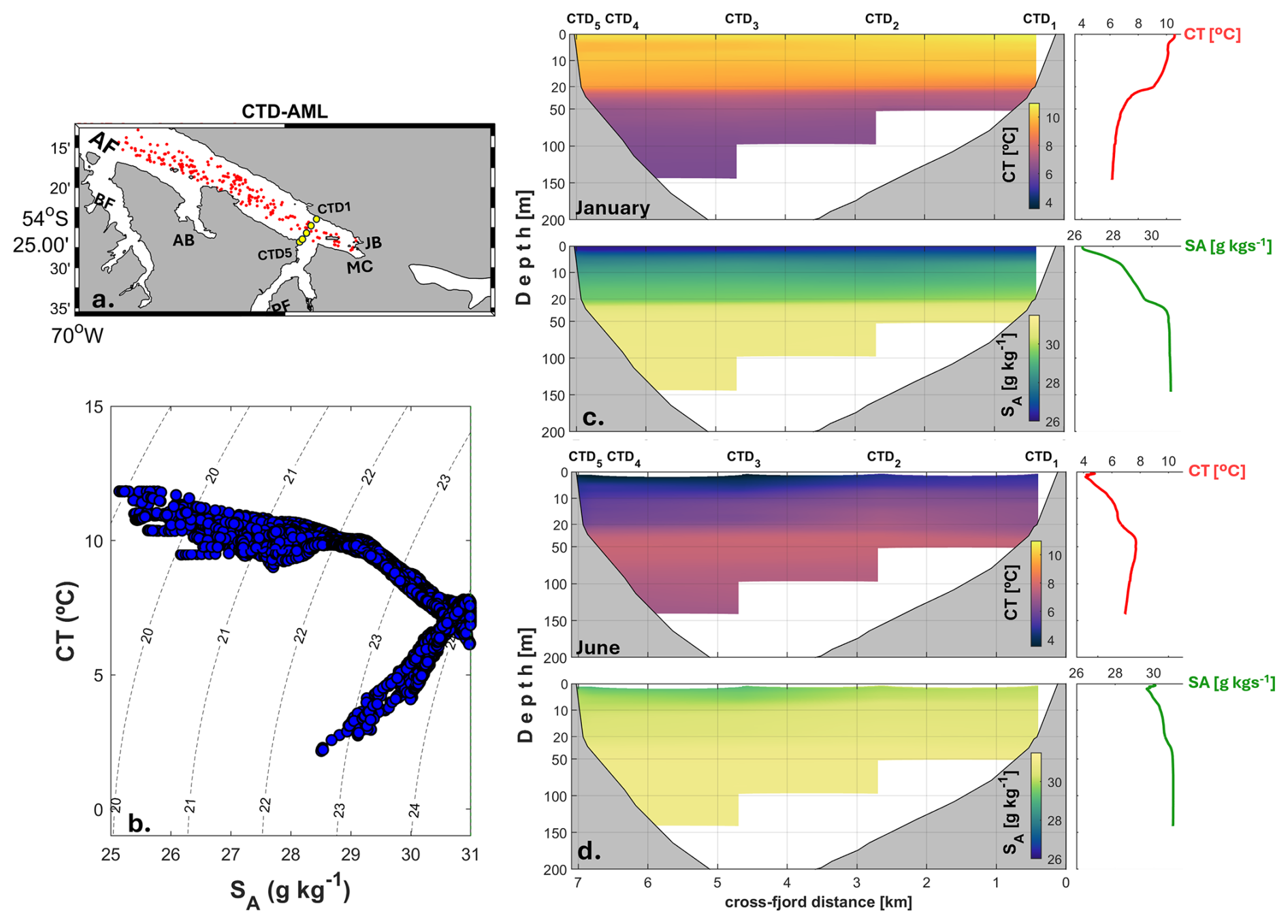
Figure 6 (a) Location of the hydrographic profiles (Absolute Salinity, S_A; Conservative Temperature, CT) acquired via CTD-AML. (b) CT/S_A diagram for the CTD-AML dataset. Segmented black lines represent conservative density anomaly (σ_CT) isopycnals in kg m⁻³. Summer and (d) Winter cross-fjord sections of S_A and CT, extending from station CTD1 (northern side) to CTD 5 (southern side) the cross-fjord stations are present in yellow circles in (a). Average vertical profiles of CT and S_A for the entire transect are displayed to the right of (c) and (d).

Both sets of hydrographic data (along-fjord and cross-fjord CT and S_A profiles) were used to estimate the Freshwater Content (FWC) and Potential Energy Anomaly (PEA) for January (summer) and June (winter) (Fig. 7). During January, the FWC exhibited a gradient, decreasing from the fjord head toward the Magellan Strait (MS). At 3.9 km from the head, which is near Parry Fjord (PF), the FWC was 1.37 m then FWC decrease trough the fjord's mouth presenting peaks events (ca. 0.6 m) near of Brookes Fjord (BF) at 71 km from the head reaching a minimum FWC of 0.14 m near the connection with the Magellan Strait (Fig. 7a). The along-fjord structure of PEA closely resembled that of the FWC, displaying a maximum of 157.2 J m⁻³ near PF and secondary maxima at 14 km (ca. 152.5 J m⁻³) and BF (ca. 71.3 J m⁻³). In June (winter), both FWC and PEA were lowers and noisy with lower values (FWC ∼ 0.2 m, PEA ∼ 7 J m⁻³) around BF location (70 km from the head) (Fig. 7b).

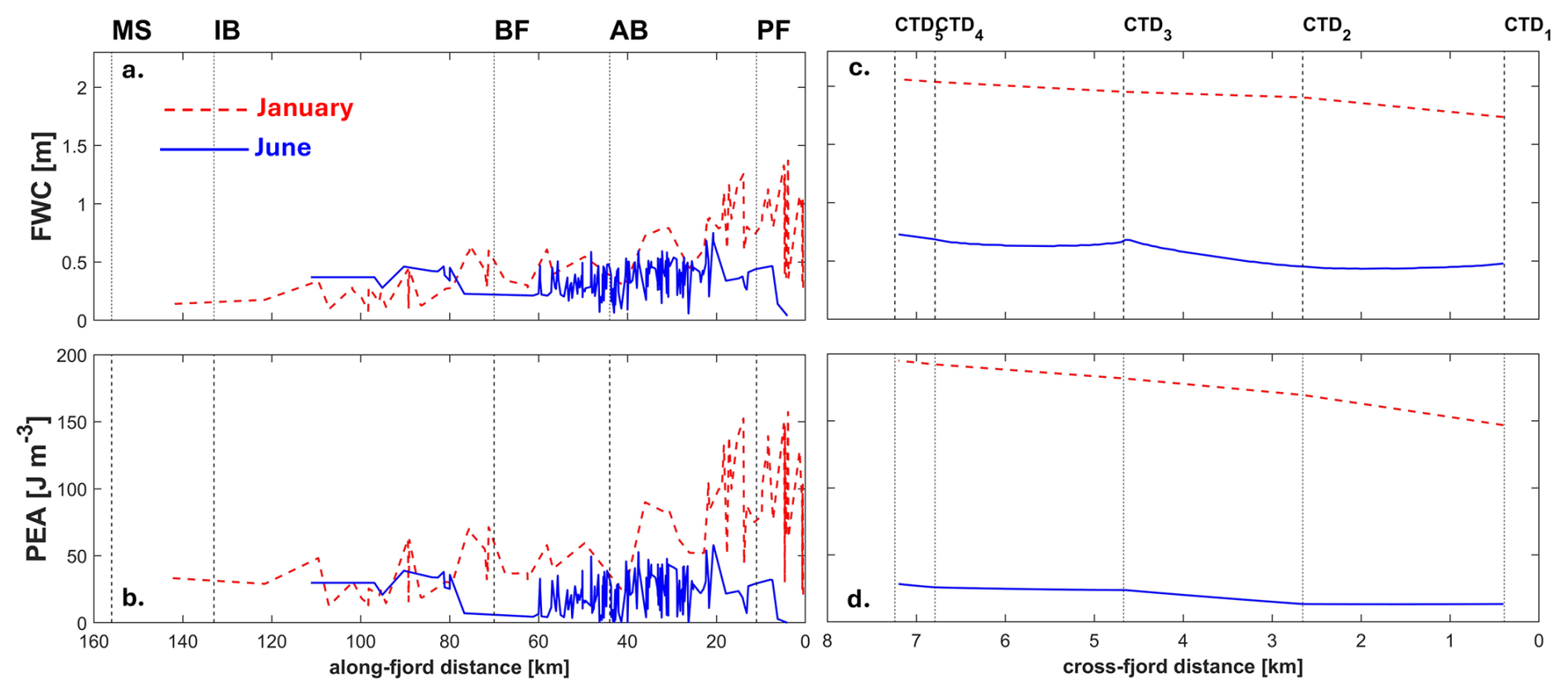
Figure 7 Distributions of Freshwater Content (FWC) and Potential Energy Anomaly (PEA) for January (dashed red line) and June (solid blue line) shown for the (a, b) along-fjord and (c, d) cross-fjord transects. Relative distance from the fjord head (along-fjord) and from the northern side (cross-fjord) is indicated with segmented thin black lines.

The cross-fjord FWC and PEA values were consistent with the along-fjord estimations, as summer values exceeded those recorded in winter. In summer, FWC ranged from 1.8 m (north side) to 2.1 m (south side), displaying a slight tilt toward the southern portion of the transect near PF (Fig. 6c). PEA values reached 200 J m⁻³ and exhibited a cross-fjord tilt analogous to that of the FWC. During the winter, FWC was less than 1.0 m and showed only a minimal cross-fjord tilt to the south. The winter cross-fjord PEA was <40 J m⁻³ a value approximately five times lower than observed in summer (Fig. 7d).

3.3.1 Temporal variability: Summer to Winter Transition

During the austral summer 2024, instrumentation measuring sea level, temperature, salinity, and oxygen was deployed at a fixed station within the Almirantazgo Fjord, Tierra del Fuego. These sensors were subsequently retrieved during fieldwork conducted at the end of June 2024. The winds-stress time series presented in Fig. 8 covers from January to June, permitting a comparison of its variability with the time series of sea level, temperature, dissolved oxygen, and salinity from the A1 mooring (Fig. 1). The following description is based on the data shown in Fig. 8.

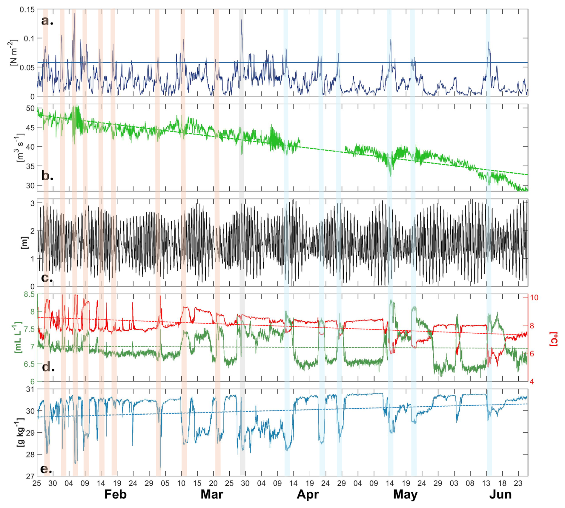
Figure 8 Time series of: (a) wind-stress magnitude; (b) Azopardo River discharge; (c) sea level; (d) near-bottom (30 m depth) Conservative Temperature (red line) and Dissolved Oxygen (green line); and (e) near-bottom (30 m depth) Absolute Salinity (blue line). Data for (c), (d), and (e) were recorded at A1 station in Maria Cove. Segmented lines on discharge, temperature, dissolved oxygen, and salinity indicate the seasonal trend for each time series. Notice that warmer events were marked with shading red, transition with shading grey and colder with shading blue.

The regional wind pattern indicated that winds persistently blew toward the fjord head, and the zonal (east–west) component was dominant across the seasons (Figs. 3, A1). Therefore, the wind-stress magnitude was analysed to characterize the variability and intensity of the winds within the fjord. The wind-stress magnitude recorded a minimum of $\mathrm{2}\times {\mathrm{10}}^{-\mathrm{4}}$ N m⁻² (6 August) and a maximum of $\mathrm{1.59}\times {\mathrm{10}}^{-\mathrm{1}}$ N m⁻² (23 July); both extremes occurred during the austral winter. The mean wind-stress for the time-series was $\mathrm{3.09}\pm \mathrm{2.26}\times {\mathrm{10}}^{-\mathrm{2}}$ N m⁻² and the 90th percentile was $\mathrm{6.24}\times {\mathrm{10}}^{-\mathrm{2}}$ N m⁻². Seasonal differences were apparent: the mean summer (December–February) wind-stress was $\mathrm{3.80}\pm \mathrm{2.26}\times {\mathrm{10}}^{-\mathrm{2}}$ N m⁻² which was higher than the mean winter (June to August) wind-stress $\mathrm{2.28}\pm \mathrm{2.16}\times {\mathrm{10}}^{-\mathrm{2}}$ N m⁻².

The wind stress time series displayed a combination of high-frequency (ca. 1 d) and synoptic (ca. 5 d) oscillations from late January (summer) to mid-April (early autumn) 2024. During this summer and early autumn phase, wind stress events exceeding 0.1 N m⁻² occurred in early February and late March. The wind pattern showed a seasonal transition from mid-April to the end of June. During this late period, oscillations were predominantly synoptic (ca. 5 to 7 d). No event surpassed 0.1 N m⁻², although notable events >0.07 were recorded in the mid-May and mid-June 2024 (Fig. 8a).

The Azopardo river discharge time series for January–June contains a data gap between 15 April and 7 May (Fig. 7). The discharge was higher in summer (48.23 m³ s⁻¹) and lower during winter (32.76 m³ s⁻¹), with a mean of 40.50±4.47 m³ s⁻¹. The data exhibited a pronounced negative seasonal trend from summer to winter, declining at a rate of −0.10 m³ s⁻¹ d⁻¹. High frequency variability was evident throughout the record; like the wind stress, daily and synoptic oscillations seemed dominant (Fig. 8b).

Sea level (SL) was derived from the pressure sensor of the NKE WiSens, SL height was referenced to the minimum recorded value to isolate amplitude and oscillations. Harmonic analysis indicated the dominance of the M₂ constituent (0.59 m), followed by K₁ (0.31 m), S₂ (0.29 m), O₁ (0.22 m), and N₂ (0.13 m). The form factor (F=0.593) confirms a mixed, predominantly semi-diurnal tidal regime. This tidal forcing accounted for 76 % of the total SL variability. An air pressure time series was not available to calculate adjusted sea level; the residual (non-tidal) variability was clearly of synoptic origin. The maximum tidal range was less than 3 m during spring tides and approximately 1 m during neap tides. Between February and June, 11 spring and 10 neap periods were observed; however, the spring tides from February to late March were less pronounced than those in autumn and early winter (Fig. 8c).

Conservative Temperature (CT) displayed a pronounced negative seasonal trend of −0.009 °C d⁻¹ from summer to winter (Fig. 8d). The maximum CT (10.23 °C) was observed during summer, while the minimum (4.98 °C) occurred in winter. The time series exhibited a mean of 7.94 ± 0.77 °C. This seasonal signal was evident in the higher mean CT during summer (8.08 ± 0.73 °C) compared to winter (7.19 ± 0.86 °C). The record was characterized by short-duration thermal events: warmer during summer (February to end of March) and colder during autumn-winter (April to June). Similarly, Dissolved Oxygen DO, showed a negative seasonal trend (−0.001 mL L⁻¹ d⁻¹) over the same period (Fig. 7d). The mean DO was 6.9 ± 0.2 mL L⁻¹ in summer and 6.8 ± 0.5 mL L⁻¹ in winter. The time series featured high DO events that were brief (<2 d) between February and mid-March but became more protracted (>2 d) during autumn and winter, with extended events (>1 week) observed from mid-May to June.

The S_A time series recorded a minimum of 27.56 g kg⁻¹ (summer) and a maximum of 30.96 g kg⁻¹ (winter) during the sampling period (Fig. 7e.). The mean S_A was 30.03 ± 0.73 g kg⁻¹ and a distinct seasonal trend (0.004 g kg⁻¹ d⁻¹) from fresher to saltier water conditions was evident between February to June. The mean summer value was 30.09 ± 0.65 g kg⁻¹ compared to winter mean of 30.46 ± 0.32 g kg⁻¹. Although the mean seasonal values were comparable, the variance in summer was four times greater than in winter. The low-salinity conditions in summer were associated with brief events (ca. 1–2 d) of <30 g kg⁻¹ waters, which occurred from late January to late March. From April to late June, these low-salinity events were more protracted (>2 d), such as those in mid-May and mid-June, but remained above 29 g kg⁻¹ (Fig. 8e).

3.3.2 Temporal Variability: Water Column Response to Wind Forcing

The summer-to-winter time series revealed a pronounced seasonal signal and provided evidence of a wind-driven response in the near-bottom (30 m) waters at the head of the Almirantazgo Fjord (Fig. 9). However, this single-depth dataset was insufficient to resolve the vertical structure of the water column's response. Consequently, the short-term mooring was deployed in Maria Cove, near the Azopardo river outflow (Fig. 1). The mooring was instrumented to record the surface and bottom (30 m) water column response to variations during contrasting wind intensity.

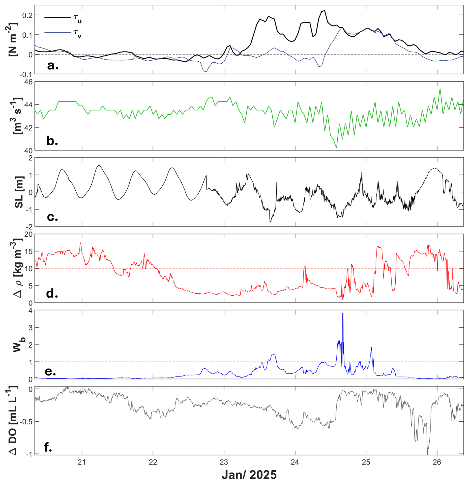
Figure 9 Short time-series acquired at mooring site A2 in Maria Cove (20–26 January 2025). Panels display, (a) along-fjord (τ_u) and cross-fjord (τ_v) wind-stress components, (b) Azopardo discharge, (c) demeaned sealevel, (d) density gradient (ρ), (e) Wedderburn number (Wb) and (f) Dissolved Oxygen gradient (DO).

On 20 January and through most of 22 January the along-fjord (τ_u) and cross-fjord (τ_v) wind-stress components exhibited low magnitudes ($<\left|\mathrm{0.05}\right|$ N m⁻²). A τ_v event (ca. −0.1 N m⁻²) occurred at the end of January 22nd, marking a transition in the time series. This event separated an initial period of weak winds (before 20:00 local time on 22 January) from a subsequent period of increased wind forcing (>0.1 N m⁻²) from 23 to 25 January (Fig. 8a). The Azopardo river discharge was relatively constant at approximately 44 m³ s⁻¹ during the weak wind period, decreasing slightly to 42 m³ s⁻¹ during the period of stronger winds (Fig. 8b). Regarding sea level, four distinct oscillations were observed during the weak wind period, presenting a clear semi-diurnal signal free of high-frequency noise. This pattern changed with the onset of strong winds, at which point the sea level record became characterized by high-frequency variability. During this latter period, the tidal oscillation was completely disrupted by the wind stress, especially between 00:00 to 12:00 (UTC−3) of 25 January (Fig. 9c).

To characterize the changes in water column density, $\mathit{\rho }={\mathit{\rho }}_{\mathrm{2}}-{\mathit{\rho }}_{\mathrm{1}}$ was used, where ρ₂ is density at 30 m and ρ₁ is the surface density. On 21 January and early 22 January, ρ exceeded 10 kg m⁻³. The gradient subsequently diminished to values near 1 kg m⁻³ and remained at this low level until the end of 24 January. At that point, where ρ increased and was maintained above 10 kg m⁻³. It decreased again to approximately 1 kg m⁻³ during the end of 25 January and the beginning of 26 January (Fig. 9d).

The Wedderburn number (Wb) was calculated using L=75 km (the basin length of AF) and h₁=20 m, the upper depth of the brackish layer (h₁). For 96 % of the deployment, events Wb remained <1. Events where Wb > 1 were observed on 23 January at 20:00. The highest values, which rose above 2 and reached a maximum of 3.77, occurred on 24 January between 20:00 and 23:00. A final event was recorded on 25 January at 02:00 (Fig. 9e).

At the beginning of the time-series (21 January to end of 23 January), the vertical Dissolved Oxygen gradient (DO) was maintained with minor variability around −0.1 mL L⁻¹. Subsequently, the gradient increased to $>-\mathrm{0.3}$ mL L⁻¹ until 12:00 (local time) on 24 January. Following this, from 12:00 on 24 January to 12:00 on 25 January, DO was approximately 0 mL L⁻¹. The most negative gradient (ca. −1 mL L⁻¹) was observed at the end of 25 January (Fig. 9f).

3.4 Spectral Analysis: pattern of variability near the bottom

The wind-stress magnitude exhibited high spectral amplitude for the oscillation with periods greater than 24 h. This diurnal band showed its greatest amplitude from late January until the beginning of May, during the winter, this band was virtually absent (Fig. 10a). The subsequent period was observed in the 3 d band, which displayed high amplitude at the beginning of the time series (25 January to 24 February) and again around 20 March and mid-May. The 10 d band was the most significant period for the wind-stress magnitude. The first two weeks of February was the only time this band showed lower amplitudes; during that period, the variability was centred at 3 d. Furthermore, distinct events with high amplitudes spanning a broad range of periods (12 to 256 h) were centred on specific dates: 5 February, 30 March, 20 April, 10 May, 3 June, and 14 June (Fig. 10a).

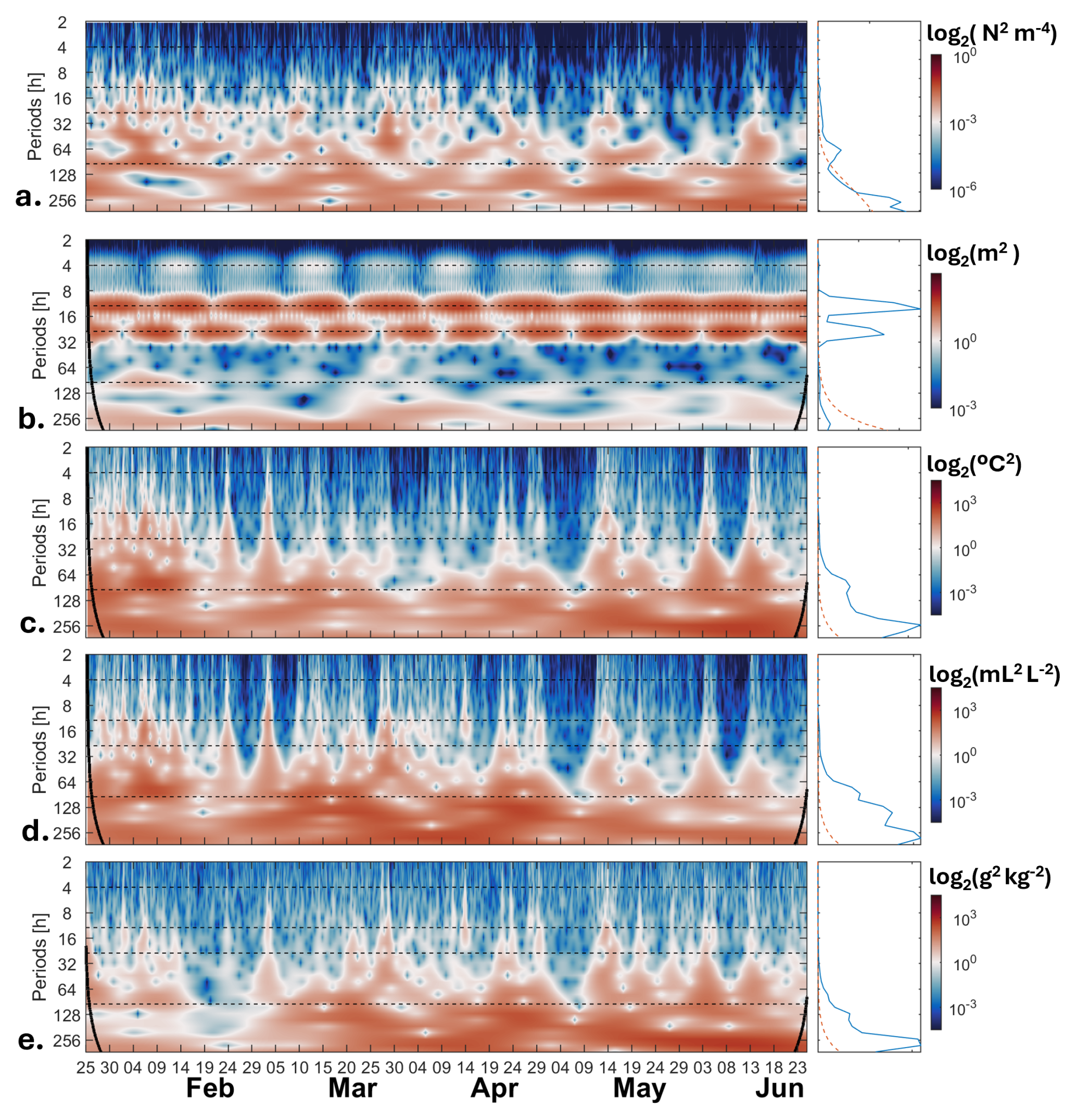
Figure 10 Wavelet analysis for the time series acquired at the A1 mooring: (a) wind stress, (b) sea level, (c) Conservative Temperature, (d) Dissolved Oxygen and (e) Absolute Salinity. For each variable, the wavelet power spectrum is shown (left panels), and the global wavelet spectrum is shown (right panels). In the power spectra, power is color-coded (red = maxima), and the black contour represents the cone of influence where edge effects become important. Horizontal dashed lines denote periods of 4, 12, 24, and 72 h.

The sea level (SL) data were dominated by tidal variability, with the highest spectral amplitudes occurring in the semi-diurnal (12 h) and diurnal (24 h) bands. Both bands exhibited a pronounced fortnightly modulation; this modulation became less distinct in the 12 h band from mid-May until the end of the time series. Other evident variability was contained at 4 h band with low amplitude and bi-weekly modulation and the low-frequency (longer than 1 d periods) which showed marked high amplitudes at 3 d (around 72 h) at the beginning of the time-series until middle of February and beginning of April. The most important (and significant) period band was centred at 10 d (256 h) into the synoptic band. This band persists along the entire time-series but diminishes its amplitude between May and June (Fig. 10b).

The CT data indicated the significance of the 3 d band. High amplitudes were observed in this band during January and February; its amplitude subsequently decreased until 3 and 14 June, when two distinct high-amplitude pulses were recorded (Fig. 9c). The global spectrum confirmed the relevance of the synoptic band, centred at 10 d (approx. 256 h). The wavelet power spectrum shows that this 10 d band was less prominent during March and April (Fig. 10c).

The DO wavelet exhibited a pattern analogous to that of CT at the start of the time series, characterized by high variability within the 3 d band. However, unlike CT, the DO data displayed high amplitudes across the 3 to 10 d bands between March and April; during this interval, the 5 d band appeared to intensify around 20 March and 24 April. Throughout the record, multiple high-amplitude events occurred across various periods (Fig. 10d).

For S_A, the time series from 23 January to 5 March was characterized by low spectral amplitudes across all periods resolved by the wavelet analysis. Following this, from March to June, high amplitudes developed at periods greater than 3 d. Within the 5-to-10 d, S_A variability initially exhibited high amplitudes centred at 5 d (late April). From mid-May until the end of the record, the dominant variability shifted to the 10 d band. High-amplitude events spanning all periods >24 h were observed centred on 3 and 13 June.

4 Discussion

The waters of the inner sea of Tierra del Fuego and the Magellan Strait are characterized by low-salinity (ca. 31 g kg⁻¹) in comparison to the adjacent Pacific Ocean and Atlantic Ocean, where salinities are approximately 34 g kg⁻¹ (Brun et al., 2020). These oceanic waters enter the inner-sea and mix with regional freshwaters inputs. Strong tides (Medeiros and Kjerfve, 1988) and strong winds are the primary mechanisms driving mixing within the region.

The study of Brun et al. (2020) identifies the hydrographic condition of the Magellan Strait as the source of the low-salinity waters observed in the Atlantic; this study attributes the mixing primarily to tidal forcing. In the atmosphere, the Southern Annular Mode and other hemispheric-scale modes exert a substantial influence on Patagonia weather (Garreaud et al., 2013). The region experiences an intensification of westerlies over Tierra del Fuego, which shows a significant positive trend during the austral summer (Garreaud et al., 2013). Local topography often channels these winds down-fjord (Oltmanns et al., 2014). This effect significantly impacts surface waters and ice, which can be driven down-fjord, subsequently promoting air-sea gas exchange and heat, and facilitating deep-water exchange within the fjords (Klymak et al., 2025).

The role of the wind promoting the deep exchange is an important dynamic component in semi-enclosed coastal systems, such as fjords, which are characterized by limited ventilation. Recent studies have documented warming and deoxygenation in the Puyuhuapi Fjord (Linford et al., 2023) and in British Columbia (Jackson et al., 2021). Fjord circulation is driven by a combination of mechanism driven by density gradient, tides, and winds. In these systems, where the upper and intermediate layers are dominated by estuarine circulation (e.g. Stigebrandt, 2012). The role of wind has been understudied compared to density and tidal drivers in fjords (Soto-Riquelme et al., 2023) and this is also the case for the inner sea of the southern Patagonia fjords. In conditions of up-fjord winds, opposing to estuarine outflow, the transference of momentum could retain or even reverse the upper outflow (e.g. Cáceres et al., 2002), this yield to a water column adjustment which drives in a three-layered residual pattern, particularly in fjords with weak tidal influence (Geyer, 1997). In systems with a strong tidally influence, deeper circulation could also generate a three-layer pattern observed in systems like Chilean Patagonia (e.g. Valle-Levinson et al., 2014). The mechanism of the formation of three or more layers in fjords has been documented by Farmer and Freeland (1983) and to verify the residual pattern of the circulation in the Almirantazgo fjord a dedicated study using ADCP data (as in Wan et al., 2017 or Castillo et al., 2012) will be required in future studies in the region.

4.1 Along-Fjord Exchange of Upper brackish Layer

The CTD-SRDL data was used in the estimations the upper outflows exchange and to determine flushing times of the same layer. The mean profiles from the along-fjord CTD-SRDL (Fig. 5c, d) and the mean profiles of the CTD-AML (Fig. 6c, d) were highly consistent between the seasons; highly stratified in January and mixed during June. Despite the fact, the study has several profiles in the region: inner the fjords and in the open ocean (see Fig. A2). In the Almirantazgo fjord, only few CTD-SRDL profiles were nearest to the cross-fjord stations (see Fig. 6a). Thus, the study was able to make a comparison for data of the 27 of January and between 6 and 9 June 2024. During those dates, CTD-SRDL data was taken nearest to CTD2 and CTD3 stations (Figs. 2, 6a). Considering that the study used a h₁=20 m during January, the comparison between upper layer (CTD depths ≤ 20 m) and deeper layer (CTD depths > 20 m) were used to quantify the agreement between CTD-SRDL and CTD-AML. The comparisons showed the best agreement for January temperatures (r>0.96). During June, the relation was lower with r>0.80 in the upper layer. The summer Salinities presented RSMD > 2.61 g kg⁻¹ with r=0.67 at CTD2 in the upper layer. In June, RMSD was lower than January (RSMD < 1.10 g kg⁻¹) with r between 0.85 (CTD2) and 0.94 (CTD3). In oceanic water, the performance change, the lowest errors and highest correlations were concentrated for profiles with depths > 50 m with RMSD < 0.3 and r > 0.8 for both temperature and salinity, indicating a good overall representation. Although the values in the surface layer were slightly lower, they remained consistently good for both variables. The low correlation in Salinity could be taken with the consideration that, (1) few profiles were able to make the comparison, (2) the dates selected were near under variable conditions of Salinity (see Fig. 8e), (3) the processing of the traditional CTD take the downcast to be analyzed, whereas CTD-SRDL record data when elephant seals are coming to surface.

Utilizing the hydrographic data acquired from two complementary sources (CTD-SRLD and CTD-AML), within the Tierra del Fuego fjord system, and considering the basin geometry, a first-order estimation of the flushing time for the upper layer (T_F) of the Almirantazgo Fjord was estimated (from MC to BF). This approximation, based on the Knudsen theorem, this requires determining the upper Volume of the brackish layer. The study shows that during January the amount of freshwater was considerably higher than June (Fig. 7), additionally cross-fjord transect shows that during January the upper brackish layer (h₁) could be as deeper as 20 m but during June was shallower, h₁=5 m (Fig. 6c, d). Similarly, the along-fjord patterns showed that during January the fjord showed a salt-wedge pattern deeper near the head and shallower (ca. 5 m) near the mouth of the fjord (Fig. 5c) in contrary, during June the upper brackish layer has a constant and shallower (ca. 5 m) along the entire fjord. These cause geometry differences for the Volume between January (right trapezoidal prism) and June (right rectangular prism). Considering the average width of AF was nearly 12 km the upper Volume (V₁) of the brackish layer was 11.25×10⁹ m³ in January whereas in June was 4.5×10⁹ m³ yields that the upper brackish layer of January was 2.5 times of June.

At the mouth of the AF (Fig. 1) the study estimates the along-fjord exchange of the upper layer, $Q_{\mathrm{1}}=A_{\mathrm{1}}\cdot v_{\mathrm{1}}$, here A₁ was the transversal area at the mouth and v₁ is the advective along-fjord current. Expanding, $A_{\mathrm{1}}=b\cdot h_{\mathrm{1}}$, taking an averaged width of 12 km and h₁=5 m the transversal area in both January and June was $A_{\mathrm{1}}=\mathrm{6}\times {\mathrm{10}}^{\mathrm{4}}$ m². This study do not take currents measurements but the Fisheries Chilean Institute (IFOP) is working to modelling the Magellan strait, they use a MIKE 3D model for modelling (http://chonos.ifop.cl/, last access: 16 June 2026) the northern Patagonia (between Puerto Montt and Golfo de Penas, see Fig. 1) and they using to estimate different operational results for decision makers (e.g. Reche et al., 2021; Ruiz et al., 2021). For the study region, the model lack in circulation validation (Cristian Ruiz, personal communication, 1 May 2026) but the IFOP give us a weekly averages circulation patterns for January and June 2024 (see Fig. A3). Using that model output, the study obtained typical v₁ to determine the upper exchange Q₁. The results showed that during, January v₁=0.3 m s⁻¹ whereas in June v₁=0.1 m s⁻¹ considering these values the output exchange in January was $Q_{\mathrm{1}}=\mathrm{1.8}\times {\mathrm{10}}^{\mathrm{4}}$ m³ s⁻¹ and during June $Q_{\mathrm{1}}=\mathrm{6}\times {\mathrm{10}}^{\mathrm{3}}$ m³ s⁻¹. Using that estimations to determine the flushing time ($T_{\mathrm{F}}=V_{\mathrm{1}}\cdot Q_{\mathrm{1}}^{-\mathrm{1}}$) of the upper layer, using this approximation T_F for January and June were similar order of magnitude of one week (Table 3). In this study high RMSD for surface Salinity could limited the precision of the Knudsen-based estimations. Despite that, the T_F quantification requires a second-order studies focusing into determine the water column exchanges using a validated circulation model. As an example, Pinilla et al. (2020) using a circulation validated model, determine the water age into the Puyuhuapi fjord obtaining longer than 1 year for intermediate and deeper waters of the fjord which could promote low DO in that region.

Table 3 Flushing times parameters for January and June. Upper ($S_{\mathrm{1}}/D_{\mathrm{1}}$) and deeper ($S_{\mathrm{2}}/D_{\mathrm{2}}$) average along-fjord Salinities/Densities, upper layer Volume (V₁), typical upper layer velocity (v₁), upper exchange (Q₁).

The calculated upper layer flushing times were relatively longer than those reported for other highly stratified systems in northern Patagonia. For instance, Castillo et al. (2016) determined an upper-layer flushing time of 3 d for the Relocavi Fjord, and Calvete and Sobarzo (2011) found a similar 5 d flushing time for waters between the Guafo mouth and Elefantes Fjord. These results indicate that the upper layer of the Almirantazgo Fjord has flushing times of approximately one week, which may promote the concentration of materials within the basin, but the limitations of the Knudsen theorem must be taken into account and to serve as a tool that supports management and decision-makers, this first-order estimation of exchange times will require validation by a second-order estimation in future works.

4.2 Freshwater Dynamics and Stratification

Traditional CTD measurements acquired near Jackson Bay during both January and June recorded salinities below 31 g kg⁻¹. Data from the time series mooring (recovered in June) further indicated that near-bottom (ca. 31 m depth) salinities reached a minimum of 27 g kg⁻¹ during the austral summer (January). This was followed by a seasonal increase, with values reaching a maximum of 30.5 g kg⁻¹ near the recovery dates in June 2024. The low salinities characteristic of the inner sea of Tierra del Fuego is attributed to the input of glacial meltwater, which exhibits strong seasonality. During summer, the along-fjord Freshwater Content (FWC) was higher in the first 20 km from the head of the fjord in the region where Parry fjord (PF) and the Azopardo river (AR) had the major influences on the freshwater input (Fig. 7a, b). Minor peaks of FWC and PEA were located at Brookes fjord (BF) suggesting the glacial melting influences on the FWC increase. Although a lack of comprehensive winter data prevents full confirmation, cross-fjord FWC measurements show that January values are at least twice as high as those observed during the June (Fig. 7a, b). This distribution is consistent with a surface slope toward the fjord head and an upper salt-wedge along-fjord structure (Fig. 5c). This typical structure of strong stratified estuaries, like fjords (Geyer and Ralston, 2011) has been documented previously in Chilean fjords like, the Reloncaví fjord (e.g. Castillo et al., 2012) and Puyuhuapi fjord (e.g. Schneider et al., 2014). The FWC has been useful to quantify the amount of freshwater input in Chilean fjords system between 43.5 to 46.5° S by Calvete and Sobarzo (2011) in this study the authors report FWC ∼ 7 m near a region with tidal-glacial influence, here FWC was < 2 m suggesting a low amount of freshwater in the Almirantazgo fjord system. The summer upper-layer salinity from the seal-borne data was less well constrained than temperature, this uncertainty propagates into the along-fjord Freshwater Content estimations.

4.3 Patterns of Variability at 30 m depth near the fjord's head

Wavelet analysis of the time series indicated a dominance of low-frequency (periods > 24 h) variability in wind-stress magnitude, Conservative Temperature (CT), Dissolved Oxygen (DO) and Absolute Salinity (S_A). The sea level (SL) was the exception (Fig. 9b), being dominated by the semi-diurnal (12 h) and diurnal (24 h) signals. This tidal dominance is consistent with the harmonics analysis and the calculated form factor (F=0.593).

In stratified systems, internal (baroclinic) seiches can be excited in the pycnocline, contributing to entrainment and enhancing heat and salt exchange between layers e.g. in the Gulmar fjord (Arneborg and Liljebladh, 2001), the Gullmaren fjord (Djurfeldt, 1987) and the Reloncavi fjord (Castillo et al., 2017). Up-fjord winds generate a surface slope ($\partial \mathit{\eta }/\partial x>\mathrm{0}$), highest at the fjord head. In stratified conditions (ρ≫1), this results in a deepening of the pycnocline at the head, creating an opposing pycnocline tilt ($\partial h_{\mathrm{1}}/\partial x<\mathrm{0}$) (Farmer, 1976). In this study, the effect of the wind over the dynamics of the fjord is the main focus thus to determine the baroclinic adjustment scale (t_s), in the Almirantazgo fjord here the study consider the length of the AF which is 75 km to determine the time required for this pycnocline tilt to be established, is defined by $t_{\mathrm{s}}\sim L/c_{\mathrm{1}}$ (e.g. Klymak et al., 2025). Here, for January conditions t_s=3.34 d whereas for June t_s=22 d. Comparing t_s with T_F (Table 3), the results indicates that during January the baroclinic adjustment is lower than the flushing time but during June, t_s>T_F suggesting that the wind-setup do not reach the quasi-steady state, probably due to the transient nature of the strong winds (Fig. 8) and the weak stratification of the water column during this month (Figs. 5 and 6) in the region.

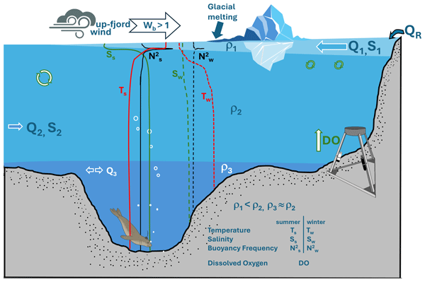
Based on the established importance of the Earth's rotation, the 6-month mooring data, the short-time mooring data, and the hydrographic surveys, a schematic fjord dynamic is proposed. Winds in the region (Maria Cove, Fig. 2) are typically persistent and directed up-fjord (see Fig. A1). These forcing tilts the surface layer ($\partial \mathit{\eta }/\partial x$) and enhances the along-fjord barotropic pressure gradient. The response is a deepening of the pycnocline at the head and shallowing at the mouth (Fig. 5c). This salinity structure is concurrently modulated by summer glacial meltwater (Fig. 7a). These freshwater forms a buoyant plume. Under weak winds, this plume would likely be deflected by the Coriolis force and exit the fjord. However, moderate to-intense up-fjord winds – acting within the baroclinic adjustment time (t_s=3.34 d) – appear to overcome this deflection, trapping the plume at the fjord head. During this process, the plume gains heat. Consequently, January up-fjord wind events are associated with pulses of warmer waters at 30 m depth (Fig. 8d). This is consistent to the observations made by Aravena-Yáñez et al. (2025) in Punta Santa Ana at the south of the Magellan Strait. The associated turbulence also increases DO and promotes mixing of the upper freshwater, which reduces the salinity of the deeper waters (Fig. 8e). This process is markedly seasonal. A regime occurred in mid-March 2024, after which wind intensity decreased, and strong events became primarily synoptic. In this early autumn period, up-fjord wind events began to be associated with colder waters. In winter, the up-fjord wind events were related to colder waters. During June, surface water resides longer (see Table 3) at the surface than in January and thus loses heat to colder overlying air. These colder events are associated with high DO, resulting from enhanced turbulence (oxygen ingress) and the higher solubility of oxygen in colder water (Fig. 8d). Observations in the short-term are consistent with the synthesis. Following a strong up-fjord wind pulse (Wb > 1), the DO gradient approached zero ($\partial \mathrm{DO}/\partial z\sim \mathrm{0}$), implying oxygenation of the layer at 30 m (Fig. 8e, f). The time-domain analysis (Fig. 8) retained the linear trends to reflect the seasonality. The decreasing river discharge trend and increasing salinity trend reflect the freshwater impact in the study region. However, the FWC estimations (Fig. 7a) suggest that freshwater inputs from glacial locations are more significant than riverine inputs. In the region, Izagirre et al. (2025) using aerial imagery between 1945–2024 showed that Darwin's Cordillera increase the number of glacial lakes and thus the freshwater input by Glacial Lake Outburst Floods (GLOFs) due to a warming progress. Although the specific volume of glacial inputs was not estimated, this study concludes that the combination of this substantial freshwater input with tidal and wind-driven mixing maintains the low-salinity conditions of the inner-sea of Tierra del Fuego.

4.4 Wind influence on the inner sea of Almirantazgo Fjord

While ERA5 reanalysis data are valuable for assessing the spatio-temporal variability of the wind forcing in southern Patagonia, comparisons with in-situ meteorological stations (e.g. Punta Arenas and Porvenir) reveal that ERA5 magnitudes are typically 20 % lower than observations. This remarks that the wind-based estimations of the study were likely conservative and thus supporting the high influence of wind-driven on the dynamics of the Almirantazgo fjord.

To assess the potential for wind-driven mixing, the dimensionless Wedderburn number (Wb) was calculated. During January, intense wind-stress in AF could be as high as τ=0.10 N m⁻² taken a mean density difference ρ=1.5 kg m⁻³ (see Table 3) an upper layer h₁=20 m and considering the AF length L=75 km the study obtained a Wb = 1.28. This value indicates that wind events can perturb the pycnocline during the stronger stratified condition of January. The June conditions were highly mixed with a ρ=0.1 kg m⁻³ and h₁=5 m, wind stress was able to perturb the pycnocline even in weakest winds conditions. For other hand, the observational data from the short-term deployment (Fig. 9e) confirm this: during highly stratified conditions, Wb repeatedly exceeded 1 and reached values as high as 3.7, demonstrating that wind is sufficient to drive dynamics at the fjord head. The h₁ depths for January and June were estimated by the cross-fjord and along-fjord maximum N² depths at the sites near of the CTD cross-fjord transects (Fig. 2). The sensitivity of the Wb parameter was assessed by calculating the wind-influenced depth $h_{\mathrm{1}\mathrm{W}}=\sqrt{\frac{\mathit{\tau }L}{\mathrm{\Delta }\mathit{\rho }g}}$. In January, h_1W=22.6 m closely aligns with the h₁=20 m used on the estimations. In June, however, h_1W=27.7 m exceeding the seasonal depth for Wb by a factor of six. Although direct validation via ADCP data was not available for this study – unlike the work of Wan et al. (2017) in Douglas Channel – the fact that Wb meets or exceeds the prescribed layer depth indicates that wind-driven forcing is a major driver of the surface layer in this system.

The time series (Fig. 9) also reveals a feedback mechanism. Strong winds, mix the upper water column, which diminishes the density gradient (ρ) (Fig. 9d). This reduction in stratification, in turn, increases the Wb (as ρ is in the denominator), enhancing the wind's mixing efficiency (Fig. 9e). Conversely, when winds weaken (due to synoptic and daily oscillations), freshwater discharge strengthens the density gradient. This re-stratification requires greater wind energy to overcome, and in the absence of strong wind, Wb returns to near-zero values (Fig. 9e). Under Wb > 1 the water column DO yields to mixing conditions (DO ∼ 0) showing a rapid response of the 30 m water column to strong winds (Fig. 9f).

To further quantify the wind's role, the power per unit area generated by the wind ($\mathrm{d}{\mathit{\phi }}_{\mathrm{W}}/\mathrm{d}t=\mathit{\vartheta }{\mathit{\rho }}_{\mathrm{a}}{c}_{\mathrm{d}}{W}_{\mathrm{10}}^{\mathrm{3}}$) available for mixing was calculated, following methodologies from Denman and Miyake (1973) and Bowden (1981). Here, ρ_a is air density (1.23 kg m⁻³), c_d is drag coefficient ($\mathrm{1.1}\times {\mathrm{10}}^{-\mathrm{3}}$) and W₁₀ is the wind magnitude at 10 m height, here the study uses the mean magnitude (5.3 m s⁻¹) and percentile 90 (p₉₀) of the magnitude (10 m s⁻¹) for the estimations. Additionally, the ϑ coefficient was determined by $\mathit{\vartheta }=\sqrt{\frac{{\mathit{\rho }}_{\mathrm{a}}{c}_{\mathrm{d}}}{\mathit{\rho }}}$ where ρ is the water density. The study determines for mean magnitude $\mathrm{d}{\mathit{\phi }}_{\mathrm{W}}/\mathrm{d}t=\mathrm{0.2}\times {\mathrm{10}}^{-\mathrm{3}}$ W m⁻² whereas for p90, $\mathrm{d}{\mathit{\phi }}_{\mathrm{W}}/\mathrm{d}t=\mathrm{1.5}\times {\mathrm{10}}^{-\mathrm{3}}$ W m⁻².

To determine if this wind power is sufficient for mixing, it must be compared to the power required to maintain stratification $\mathrm{d}{\mathit{\phi }}_{\mathrm{E}}/\mathrm{d}t$ by the estuarine circulation (Simpson et al., 1990). This stratification power is given by: $\mathrm{d}{\mathit{\phi }}_{\mathrm{E}}/\mathrm{d}t=(\mathrm{1}/\mathrm{320})(g^{\mathrm{2}}{h}_{\mathrm{1}}^{\mathrm{5}}/A_z\mathit{\rho })(\partial \mathit{\rho }/\partial x{)}^{\mathrm{2}}$. Following Osborn (1980), the vertical eddy diffusivity is parameterized as $K_z=\mathrm{0.2}(\mathit{\epsilon }/N^{\mathrm{2}})$. Based on microstructure measurements from winter 2024 (Rojas-Celis et al., 2025), we assume a representative dissipation rate of $\mathit{\epsilon }\sim O\left({\mathrm{10}}^{-\mathrm{6}}\right)$ W kg⁻¹ and typical buoyancy frequency of N²=0.0028 s⁻² which yields $K_z\sim \mathrm{7}\times {\mathrm{10}}^{-\mathrm{5}}$ m² s⁻¹.

The relationship between the vertical mixing of momentum and scalars is governed by the turbulent Prandtl number (${\mathit{Pr}}_t=A_z/K_z$; Thorpe, 2005). Assuming the standard Reynolds analogy for neutral or weakly stratified flows (Pr_t=1; Mellor and Yamada, 1982; Rodi, 1987), the resulting eddy viscosity (A_z=K_z) yields a stratification power of $\mathrm{d}{\mathit{\phi }}_{\mathrm{E}}/\mathrm{d}t=\mathrm{21}\times {\mathrm{10}}^{-\mathrm{3}}$ W m⁻². This value is one order of magnitude higher than wind power ($\mathrm{d}{\mathit{\phi }}_W/\mathrm{d}t$), which would imply that wind forcing is insufficient for mixing. However, the Pr_t=1 assumption breaks down under stratified environments where buoyancy forces supress scalar mixing more efficiently than downward momentum transport (e.g. Munk and Anderson, 1948; Venayagamoorthy and Stretch, 2010). Consequently, in highly stable flows, Pr_t increases significantly, often reaching values O(10) (e.g. Pacanowski and Philander, 1981; Peters et al., 1988). Applying a scaling of Pr_t=10 to the summer conditions in the Almirantazgo fjord yields an effective eddy viscosity $A_z\sim \mathrm{7}\times {\mathrm{10}}^{-\mathrm{4}}$ m² s⁻¹. This reduces the estuarine stratification power to $\mathrm{d}{\mathit{\phi }}_{\mathrm{E}}/\mathrm{d}t=\mathrm{2.1}\times {\mathrm{10}}^{-\mathrm{3}}$ W m⁻².

Under these physically constrained parameterizations, first-order approximations indicate that estuarine stratification power becomes comparable to the wind power during intense episodic winds events of up to 9 m s⁻¹ ($\mathrm{d}{\mathit{\phi }}_W/\mathrm{d}t=\mathrm{1.2}\times {\mathrm{10}}^{-\mathrm{3}}$ W m⁻²). This scaling suggests that despite the high static stability of the water column, wind momentum can be sufficiently transferred downward to overcome stratification and induce mixing. Nonetheless, these steady-state assumptions warrant further validation through future observational and numerical studies to better constrain the spatiotemporal variability of mixing in the fjord.

Despite the dominant tidal forcing in the Magellan Strait (Fig. 3) and the strong salinity-driven stratification from glacial melt (Figs. 4c, 5c, 6a, c), the wind is a critical mixing agent. Both the Wedderburn number analysis and the mixing power comparison confirm the wind's capacity to mix the upper water column. This study provides the first quantification of the wind-driven effect in one of the southernmost fjord of Chile (Fig. 10).

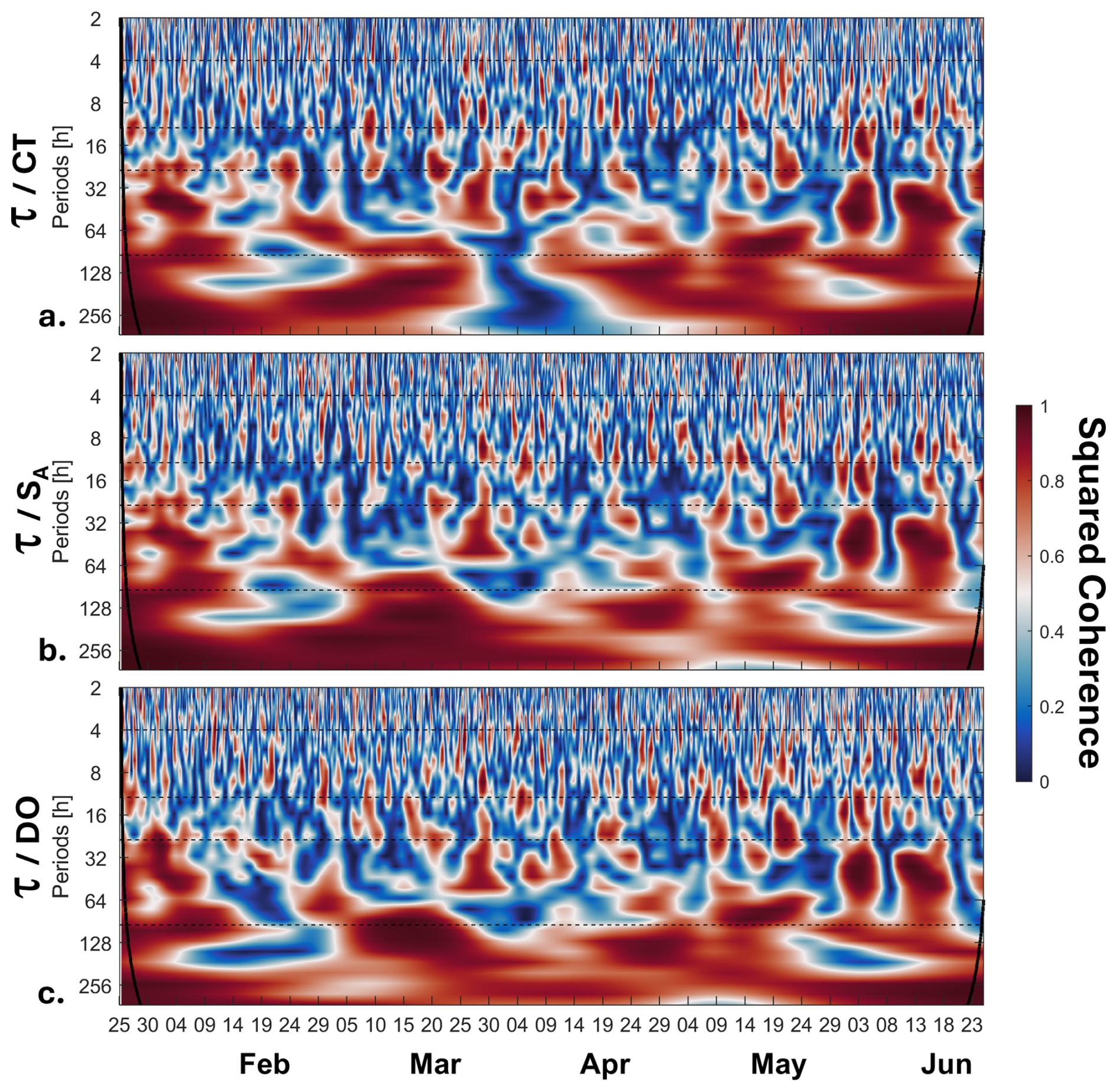
Figure 11 Squared coherence wavelet spectrums, between τ (wind-stress) with (a) Conservative Temperature (CT), Absolute Salinity (S_A) and Dissolved Oxygen (DO) for the time series acquired at the A1. Horizontal dashed lines denote periods of 4, 12, 24, and 72 h.

Wind stress in the study area showed significant squared coherence with CT, SA, and DO at periods greater than 16 h, exhibiting marked synoptic variability at periods exceeding 70 h (Fig. 11). The most intense events (>0.07 N m⁻²; Fig. 8) were highly coherent within the 24–72 h band, suggesting that synoptic wind forcing drives a uniform response in hydrographic properties at 30 m near the fjord head. Interestingly, CT coherence for periods >64 h showed a distinct dip centered on 4 April 2024, despite remaining high during the surrounding periods (Fig. 11a). This indicates a temporary shift in the CT response to wind forcing between 30 March and 9 April, which resulted in the observed breakdown in coherence between the variables.

In the context of climate change and the projected intensification of the Southern Hemisphere westerlies, these findings are critical. The Almirantazgo Fjord ecosystem, with a seasonal stratification of the upper layer and mixing processes dependent on both tides and wind, will be profoundly influenced by future atmospheric changes. Therefore, while tidal and buoyancy forces establish the baseline conditions, the answer to the fjord's physical and ecological future is unequivocally linked to the wind.

5 Conclusions

The hydrodynamics of the inner sea of Tierra del Fuego are primarily controlled by the seasonal cycle of glacial freshwater input, which establishes strong stratification during summer and modulates upper layer renewal rates. This buoyancy forcing drives a circulation characterized by rapid upper-layer flushing time in the order of one week. While M₂ tidal energy dominates the adjacent Magellan Strait, our analysis confirms that the specific dynamics of the Almirantazgo Fjord are governed by the interplay between this glacial freshwater buoyancy and along-fjord wind stress.

A key contribution of this study – supported by unprecedented spatial coverage from instrumented southern elephant seals – is the quantification of wind-driven mixing. The frequent occurrence of Wedderburn numbers >1 (peaking at 3.7) provides direct evidence that synoptic wind events are sufficient to destabilize the pycnocline.

Ultimately, these physical processes have critical biogeochemical consequences. The observed oxygenation at 30 m depth of the fjord's head following strong up-fjord wind pulses indicates that atmospheric forcing is essential for ventilating the inner bay at the head of the fjord. As climate change projects an intensification of the Southern Hemisphere westerlies, the physical and ecological future of this fjord system will be increasingly defined by its sensitivity to wind-driven mixing.

Appendix A

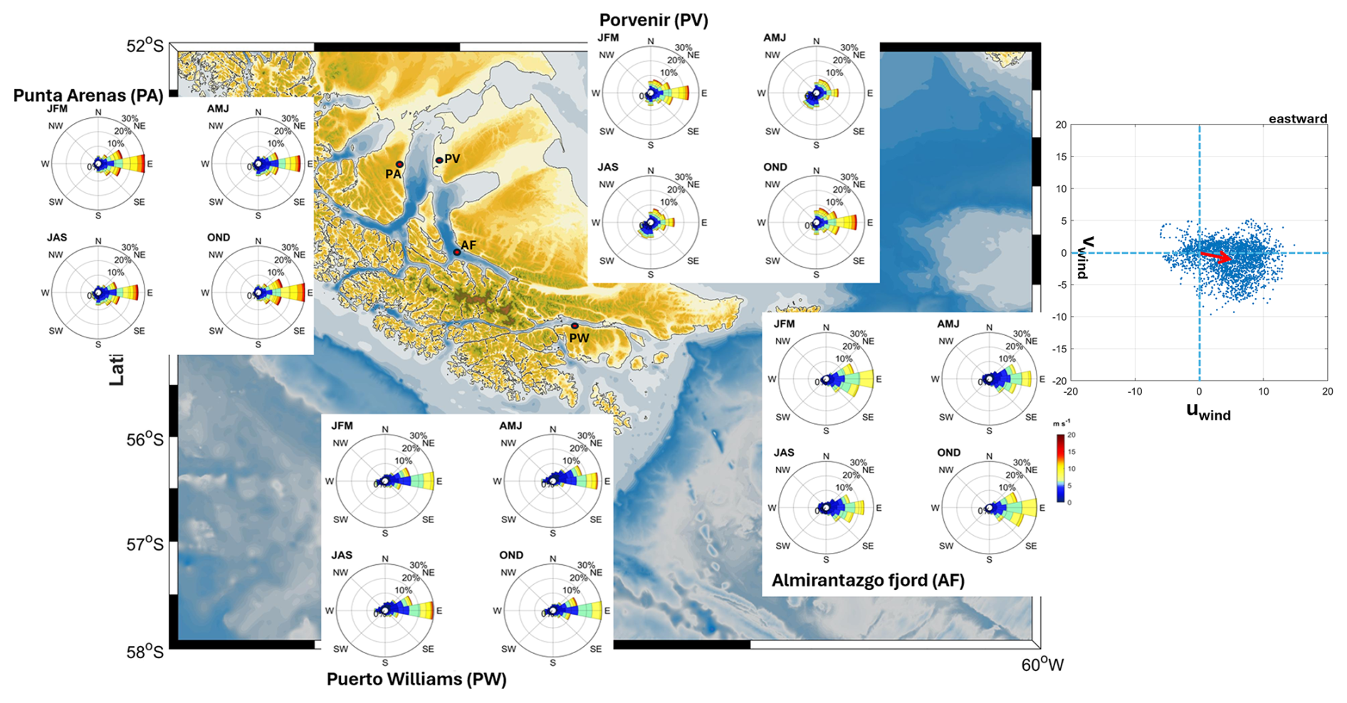
Figure A1 Regional wind climatology for the 1970–2024 period. Wind direction follows the oceanographic convention (indicating the direction towards which the wind blows).

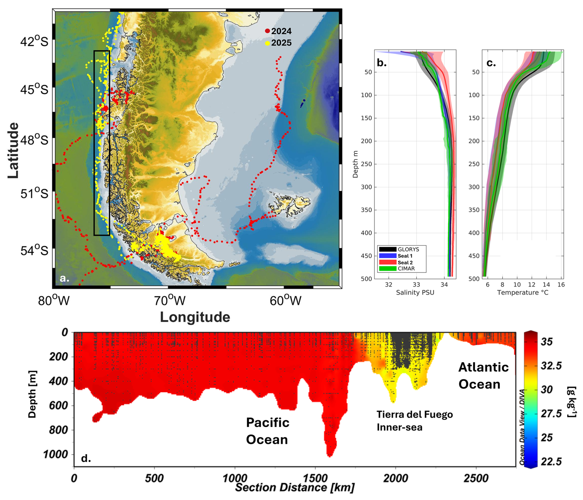
Figure A2 (a) Elephant seal trajectories within the Patagonian fjords and channels during 2024 (red dots) and 2025 (yellow dots). Comparison of CTD-SRDL (b) salinity and (c) temperature data with is situ observations (CIMAR) and GLORYS model outputs for the defined by the rectangle in (a). (d) Absolute Salinity of a transect between the Pacific Ocean, the Tierra del Fuego inner-sea, and the Atlantic Ocean. GLORYS ocean reanalysis data © Copernicus Marine Service.

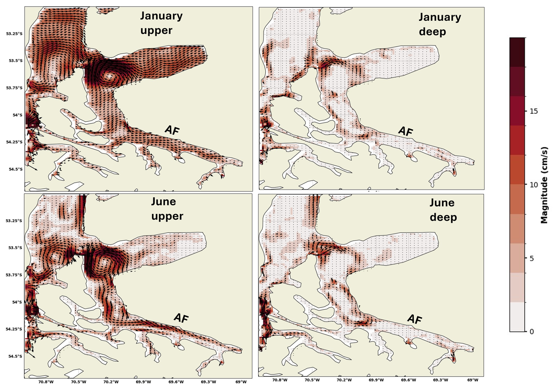
Figure A3 MIKE 3D output model of IFOP – CHONOS. Upper and deeper circulation in the study region to determine the exchange fluxes in the Almirantazgo fjord (AF).