A Digital Twin Ocean: can we improve coastal ocean forecasts using targeted marine autonomy?

This study outlines the development and testing of a Digital Twin Ocean (DTO) framework, aimed at improving coastal ocean forecasts through the use of autonomous underwater gliders. A fleet of gliders were deployed in the western English Channel during August-September 2024 to collect measurements of temperature, salinity, chlorophyll and oxygen, aiming to track the movement of the harmful algal bloom Karenia mikimotoi. Measurements were assimilated into a very high resolution (1.5 km) numerical forecast model, with an implementation of biogeochemistry data assimilation for this purpose. The model forecast was then used by a probabilistic uncertainty model to plan a series of waypoints to navigate the glider fleet towards features of interest. By utilising a continuous feedback loop of measurement, prediction, guidance, and refinement a system with real time coupling between the real ocean environment and its digital counterpart has been established.

Building upon a prior pilot study of Ford et al. (2022), this work improves every element of the system to address several limitations of the prior configuration. Whilst a bloom was present in the wider area, measurements and modeling suggest it didn't enter the glider operation zone. Despite this and other operational challenges the mission clearly demonstrates the benefits of such a system. The ability to simultaneously track multiple features of interest, namely chlorophyll maxima and oxygen minima, would not have been possible with a single glider resulting in significant benefits to the system. Furthermore, the improvement to biogeochemical forecasting has been demonstrated through a series of post mission experiments, highlighting the advantages of high temporal resolution observations and increased spatial resolution of the model.

1 Introduction

Digital twins of the ocean (DTO) are emerging as a key area of marine science research (e.g. Tzachor et al., 2023), reflected by a range of international activities including the UN Ocean Decade programme Digital Twin of the Ocean (DiTTO, https://ditto-oceandecade.org/, last access: 23 June 2026) and the European Digital Twin of the Ocean (European DTO, https://digitaltwinocean.mercator-ocean.eu/, last access: 23 June 2026). DTOs are often understood as digital replicas of the real-world ocean, where information flows in both directions, between the real and virtual, or digital twin. This two-way flow is typically used to allow near real-time decision making purposes in a highly changeable environment, where adaptive monitoring and data delivery that continually updates and improves the digital twin is beneficial (Tzachor et al., 2023). The coastal ocean region is vital to communities around the world, with fisheries and tourism amongst the industries that rely on them. Therefore the ability to accurately replicate these zones through DTOs has essential real world applicability and impact. A key component to DTOs is a level of marine autonomy (Ford et al., 2022), which allow for targeted adjustments to regions and periods of observational interest through navigating marine autonomous systems (MAS) to those areas. In-situ observations of the ocean are difficult and costly to obtain, with the potential to miss vital information in an ever changing environment. Using targeted MAS offers opportunities to reduce the cost and environmental footprint of observational science by making our observations more efficient through the use of low-carbon autonomous platforms, such as ocean gliders (Testor et al., 2019). Whilst DTO capability in marine autonomy is still in its infancy, there have been demonstrations of their effectiveness for marine physics applications (Lee et al., 2022; Raza et al., 2022; Buck et al., 2024) and to some degree in marine biogeochemistry (Ford et al., 2022; Halvorsen et al., 2026).

More specifically, the study of Ford et al. (2022) applied a DTO approach to a single glider-based observational mission to track the onset of phytoplankton blooms in the wider coastal region of the western English Channel. The use of gliders within this DTO was essential, as the spatial and temporal resolution with which a glider is capable of observing in a highly dynamical coastal environment is unprecedented. That DTO design was based on assimilating glider data alongside satellite and other in situ data in near-real time into a modified version of the Met Office's operational North-West European Shelf (NWES) forecasting system (e.g. O'Dea et al., 2017; King et al., 2018; Skákala et al., 2018, 2021). This provided 2-day forecasts to an independent path-planning machine learning (ML) module that produced future navigational waypoints for the glider to optimise the probability of observing and later predicting a phytoplankton bloom. That DTO system thus provided the glider with full autonomy¹, guided by the AI decision-making process using the information cycled between all available components in real time. The study of Ford et al. (2022) demonstrated the benefits of a fully automated and adaptive observing system. The study also revealed several limitations with the approach taken, which included: (i) identified biases between different observational sources (i.e. satellite and glider) used in the data assimilation, (ii) a relatively coarse spatial horizontal resolution (7 km) of the operational model, which was too far from the horizontal spatial scales of glider daily operations given they typically travel about 1.2 km h⁻¹, and (iii) the limitation of a single glider, targeting a single feature of interest and constrained to a small operational area which constrained the range of unknowns that we could feasibly address within such a dynamic and spatially heterogeneous environment. Further demonstration of the limitations of coarse resolution is provided in Sect. 3.3.

In this work we substantially improve upon the design of Ford et al. (2022) by addressing the three issues highlighted above and deliver a full DTO demonstrator in a dynamic coastal system. The focus for our DTO demonstrator was a re-occurring bloom of a toxic phytoplankton species, Karenia mikimotoi, in the western English Channel (Barnes et al., 2015). The toxins released by Karenia mikimotoi are known to be able to kill fish (Tangen, 1977; Silke et al., 2005; Satake et al., 2005), and have other possible side-effects such as de-oxygenation or even hypoxia and reduced irradiance. The Karenia bloom has been repeatedly detected within the western English Channel region in late Summer-early Autumn (Barnes et al., 2015), and regional satellite-based detection capability has been developed to monitor its onset (Shutler et al., 2012). The highly dynamic nature and short time scales associated with such blooms make this an ideal but challenging test for our near real-time DTO approach. The glider sensors can detect total chlorophyll a concentrations (in mg m⁻³) obtained from fluorescence measurements. Such measurements however, cannot currently be unambiguously related to Karenia species biomass, despite chlorophyll a concentrations being commonly used to provide an indication for total phytoplankton biomass. So while this can provide a valuable indicator related to Karenia blooms, complementary information is beneficial to provide an early warning system based on satellite or in situ fluorescence data alone. Furthermore, substantial phytoplankton blooms occurring in stratified relatively shallow waters can lead to excess microbial oxygen consumption, during remineralization of sinking matter near the sea bottom, potentially decreasing dissolved oxygen to harmful levels. This along with successful glider based studies investigating dissolved oxygen dynamics in similarly energetic shelf seas (Williams et al., 2022, 2024) motivated us to include dissolved oxygen concentration as an additional key target observation pursued by the DTO.

The DTO presented here aimed to test the system capability to track areas of high chlorophyll and low oxygen over 2-months during the August–September 2024 period, with the hope of capturing a Karenia bloom and associated deoxygenation. It was based on a finer spatial resolution model (1.5 km) compared to Ford et al. (2022), utilised a fleet of three gliders and implemented a more advanced path planning methodology.

The 1.5 km spatial resolution system for the NWES, even though run operationally for marine physics (Tonani et al., 2019), has so far not been applied with marine biogeochemistry with data assimilation, so this is an entirely new development and major advance in shelf sea ecosystem modelling that is delivered within this DTO. The fleet of gliders was optimized for complementary purposes, i.e. to simultaneously track phytoplankton maxima and near seabed dissolved oxygen minima, resolving their temporal and spatial variability. This manuscript outlines a proof of concept for the deployment of a fully autonomous, coordinated, fleet of gliders capable of adaptively tracking multiple interconnected processes in a highly dynamical coastal environment. The design of the DTO is outlined in Sect. 2, followed by a series of post-mission experiments to analyse the impact of glider assimilation (Sect. 3.2) and resolution (Sect. 3.3) on the numerical forecasting component before discussing the effect on path planning in Sect. 3.4. As part of the development of this system, a set of data architecture and pipelines were created to make this and future work possible, which is discussed in Mansfield et al. (2025).

2 Modelling System

2.1 Digital Twin Design

The digital twin used in this study is a cyclical system of observation-prediction-navigation, shown schematically below:

Scheme 1 Cyclical digital twin ocean design.

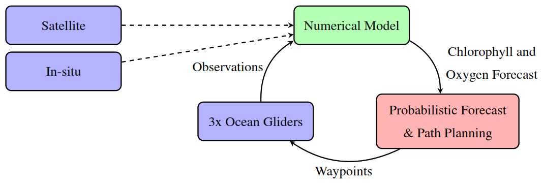
Up to 3 ocean gliders collect high-resolution depth profiles of temperature, salinity, chlorophyll and dissolved oxygen which are transmitted and received whilst the gliders are at the surface. These measurements, along with satellite observations of surface chlorophyll, temperature, and sea level anomaly, and other sources of in situ temperature and salinity observations, are assimilated daily into a numerical model which then produces a multi-day forecast. That forecast informs a probabilistic forecast and path planning algorithm to navigate the gliders during the subsequent 24–48 h. The various operating domains are shown in Fig. 1.

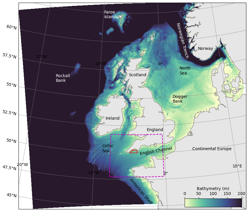
Figure 1 Bathymetry of AMM15 domain area used for the numerical model, showing the extracted region used in the probabilistic forecast (magenta dashed) and the glider operational zone (red).

2.2 Observing platforms

2.2.1 Ocean Gliders

As part of the mission, three shallow-water-rated, buoyancy driven Teledyne Webb Slocum G2 ocean gliders (units 480, 481, and 482) were deployed from the Western Channel Observatory’s L4 station on 6 August 2024. Each glider was equipped with a Sea-Bird GPCTD sensor, an Aanderaa oxygen optode, and a SeaOWL fluorometer to collect high-resolution vertical profiles of temperature, salinity, dissolved oxygen, and chlorophyll a fluorescence. Sensor models, sampling frequencies, and platform details for each glider are summarised in Table 1.

Table 1 Platform type, sensor models, and sampling frequencies for each Slocum G2 glider deployed during the experiment. The oxygen optode on unit 482 was not operational.

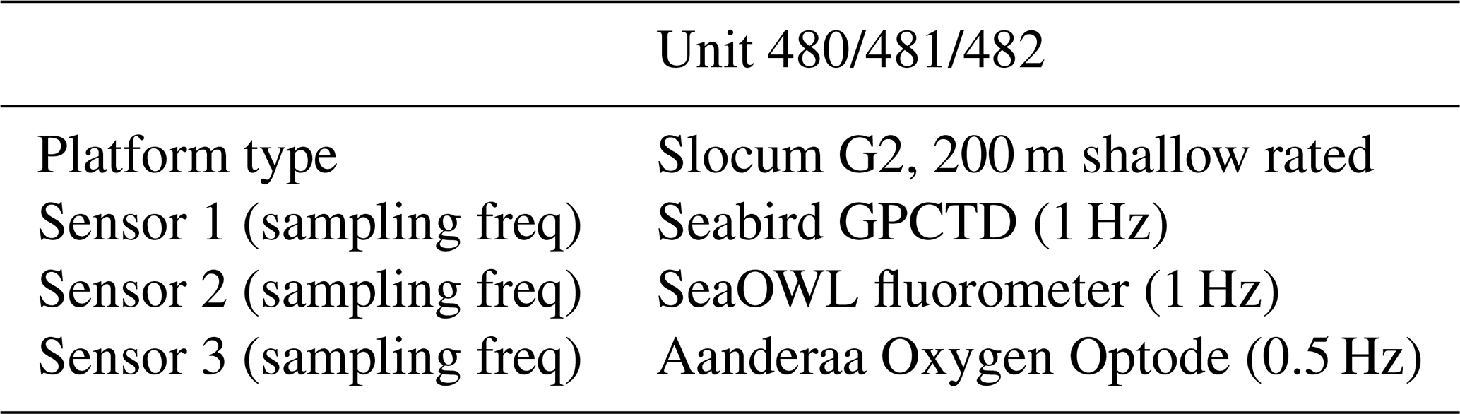
The dissolved oxygen optode connection on 482 malfunctioned during deployment, preventing the collection of any dissolved oxygen measurements from this vehicle, while the other two gliders were equipped with functioning oxygen optodes. Throughout the campaign, dive and climb profile data were transmitted ashore every six hours at full resolution (1 Hz or 0.5 Hz, depending on the sensor). Given typical vertical speeds of approximately 0.1 m s⁻¹, this corresponds to a vertical resolution of approximately 0.1–0.2 m. Successive transmitted vertical profiles were typically separated by approximately 3–5 km horizontally, depending on ambient currents and vehicle speed.

Following deployment, the gliders were manually piloted by human operators for 10 d, after which the autonomous path-planning algorithm produced the waypoints to navigate the vehicles depending on their respective tasks. During the manual pilot period gliders crossed paths several times, sampling the same areas to calibrate the sensors and reduce observational uncertainty. Handover between the path-planning and navigation of gliders was tested and performed under continued human supervision to ensure the safety of the gliders and other sea users and traffic.

Near-real-time (NRT) processing included the application of manufacturer calibrations and corrections for thermal lag. A correction for photochemical quenching was implemented on 30 August 2024, prior to this, daytime Chl a data were flagged as bad. NRT quality control was managed using adapted Argo processing routines (Wong et al., 2023; Schmechtig et al., 2023). In addition, concurrent inherent optical property measurements were used as independent reference to support manual calibration of glider-derived Chl a data, although this was not integrated into the automated processing chain. A simplified approach was attempted to account for oxygen optode response time effects; however, this proved difficult to implement robustly due to the slow optode response. Appropriately corrected and flagged data were made available via an ERDDAP server to support daily assimilation and facilitate ongoing model–data integration.

Following recovery of the gliders, full delayed-mode data processing was conducted using established oceanographic correction methods (Garau et al., 2011; Bittig et al., 2014). This included corrections for pressure offset, clock drift, vehicle navigation and application of factory calibrations. We further corrected conductivity data for thermal inertia effects (Garau et al., 2011), and dissolved oxygen data were corrected for optode response time effects and associated hysteresis following Bittig et al. (2014). Any remaining offsets were assessed through cross-validation against concurrent observations.

2.2.2 Satellite

The Ocean Land Colour Instrument (OLCI), carried onboard the Copernicus Sentinel 3A and Sentinel 3B satellites was used to calculate surface chlorophyll concentration. Data was downloaded from ESA at Level 1 and the Polymer software for atmospheric correction (Steinmetz et al., 2011) was used to produce remote sensing reflectance, with the IDEPIX plugin to the SNAP software used to identify and mask out clouds and cloud shadow. Chlorophyll was calculated from the remote sensing reflectance using the OC5CI algorithm. This is a combined algorithm as the OCI algorithm performs better in clear water (case-1), which corresponds to chlorophyll below 0.1 mg m⁻³, whilst OC5 is better in turbid waters (case-2), where chlorophyll is above 0.15 mg m⁻³. In between the results of the two algorithms are interpolated to give the OC5CI value.

During the operational mission the ESA Near Real Time Level 1 data were used in order to provide the data in a timely manner for assimilation into the numerical model. At the end of the mission delayed mode Non Time Critical data were used to provide improved accuracy. For the delayed data, Level 1 product is mapped to a gridded product at 300 m resolution, with a single composite containing all the passes over the area of interest for each day.

The Sea and Land Surface Temperature Radiometer (SLSTR) carried onboard the Copernicus Sentinel 3A and Sentinel 3B satellites was used to calculate Sea Surface Temperature. Data were processed from EUMETSAT Level 2 data (Processing Baseline 3.7) by NEODAAS to create a single dataset for each day at 1 km resolution, taking the median over day and night passes. These data were used to provide additional context during the glider deployment, but were not assimilated by the numerical forecast model which instead assimilated SLSTR SST observations processed by GHRSST (see Sect. 2.2.3).

Satellite data processing was carried out by the Natural Environment Research Council (NERC) Earth Observation Data Analysis and AI Service (NEODAAS).

2.2.3 Other Data Sources

In addition to the profiles from mission gliders and surface ocean colour from satellite, the physics observations assimilated were the same as in the Met Office’s operational AMM15 forecasting system (Tonani et al., 2019). These were satellite SST observations from various sensors downloaded from the Group for High Resolution Sea Surface Temperature (GHRSST), satellite sea level anomaly from various sensors downloaded from the Copernicus Marine Service, and in situ SST and temperature and salinity profiles downloaded from the Copernicus Marine Service and the Global Telecommunication System (GTS). These were processed, quality controlled and bias corrected as described by Tonani et al. (2019).

2.3 Numerical Forecast Model

A physical-biogeochemical model, NEMO-FABM-ERSEM, with assimilation of observational data, was used to produce daily forecasts of the physical and biogeochemical state of the NWES. The set-up was based on the NWES configurations of the Forecasting Ocean Assimilation Model (FOAM) used for daily marine forecasting at the Met Office (FOAM-NWSO and FOAM-NWSBGC).

The physical component is based on version 3.6 of the Nucleus for European Modelling of the Ocean (NEMO, Madec and the NEMO team, 2016), specifically the AMM15 CO8 configuration (Graham et al., 2018; Tonani et al., 2019) which covers the NWES at a horizontal resolution of 1.5 km. The vertical grid has 51 levels on a hybrid z-sigma terrain-following coordinate system (Siddorn and Furner, 2013). Atmospheric conditions at the surface were derived from the European Centre for Medium Range Weather Forecasting Integrated Forecasting System using CORE bulk formulae, as described by Tonani et al. (2019). The lateral boundary conditions for physical variables at the Atlantic boundary were taken from a Met Office global operational model and at the Baltic boundary from the Baltic Sea Analysis and Forecast product from the Copernicus Marine Service. In a later part of the investigation, the run was repeated using the AMM7 CO6 configuration (O'Dea et al., 2017; McEwan et al., 2021), which has a lower horizontal resolution, 7 km, but the same vertical grid. Lateral boundary conditions used the same sources as for AMM15, but surface forcing was derived from the Met Office global coupled numerical weather prediction system, as described by Tonani et al. (2019). Both AMM15 and AMM7 are run operationally at the Met Office, but only AMM7 is routinely run with a coupled biogeochemical model. This is the first demonstration of AMM15 with assimilation of biogeochemical observations.

The biogeochemical component of the forecasting model was the European Regional Seas Ecosystem Model (ERSEM, Butenschön et al., 2016), which operates on the same numerical grid as NEMO. NEMO is one-way coupled to ERSEM using the Framework for Aquatic Biogeochemical Models (FABM, Bruggeman and Bolding, 2014), with ERSEM run at each NEMO timestep in each grid cell. ERSEM is a lower trophic level ecosystem model that includes pelagic plankton and benthic fauna (Blackford, 1997). ERSEM splits phytoplankton into four functional types largely based on their size (Baretta et al., 1995): picophytoplankton, nanophytoplankton, diatoms and dinoflagellates. ERSEM uses variable stoichiometry for the simulated plankton groups and the biomass of each phytoplankton functional type (PFT) is represented in terms of chlorophyll, carbon, nitrogen and phosphorus, with diatoms also represented by silicon. ERSEM predators are composed of three zooplankton types (mesozooplankton, microzooplankton and heterotrophic nanoflagellates), with organic material being decomposed by one functional type of heterotrophic bacteria. The ERSEM inorganic component consists of nutrients (nitrate, phosphate, silicate, ammonium and carbon) and dissolved oxygen. The carbonate system is also included in the model, with total alkalinity and dissolved inorganic carbon as state variables.

Observations were assimilated daily using a 3DVar configuration of the NEMOVAR assimilation scheme (Mogensen et al., 2009; Waters et al., 2015; King et al., 2018). This used a first guess at appropriate time method to assess model-observation differences, with model values interpolated to observation locations at the nearest model time step to the time of observation. Similar to the existing operational approach for ocean colour (Ford et al., 2012), the median value for glider measurements of chlorophyll, oxygen, temperature and salinity in each model grid cell are taken every 6 h. Daytime chlorophyll values were not used, to avoid problems with fluorescence quenching. Background and observation error standard deviations for chlorophyll were the same as those used in the AMM7 operational system (Skákala et al., 2018), interpolated to the AMM15 grid. For oxygen a constant background to observation error ratio of 3 to 1 was used. Temperature and salinity from the mission gliders are assimilated alongside profiles available in other parts of the domain using the same scheme as the operational AMM15 model (Tonani et al., 2019). The correlation length scale used for chlorophyll and oxygen is the same as that for temperature in the operational AMM15 model (King et al., 2018). Satellite values of chlorophyll concentration were provided as a combination of multiple passes for each day, so are taken to be valid at 12:00 UTC, the approximate time of satellite overpass. Increments for all variables are calculated using NEMOVAR and applied to the model using incremental analysis updates. For more information on the data assimilation see King et al. (2018); Tonani et al. (2019); Skákala et al. (2021).

2.4 Probabilistic Forecasting & Path Planning

The AI-driven path planning comprises two components: (a) a novel short-term stochastic forecast model which takes the deterministic numerical forecast to derive a probabilistic forecast of Chl a and dissolved O₂ within the operational region, and (b) a path planning concept which utilises the probabilistic forecast information to yield the most useful paths fit for the science and operational purpose for the multiple gliders.

The short-term probabilistic forecast is based on Bayesian methods, which offer several advantages including incorporation of prior knowledge, intuitive uncertainty quantification, and effective modelling of spatial and temporal dependencies (Blangiardo et al., 2013; Lindgren and Rue, 2015; Salim et al., 2025; Palmí-Perales et al., 2025; Wang et al., 2025; Skakala et al., 2023). Specifically, we use the Integrated Nested Laplace Approximation (INLA) method (Blangiardo et al., 2013), combined with the Stochastic Partial Differential Equation (SPDE, Lindgren et al., 2011). This approach is a computationally efficient method for both spatial and spatio-temporal models (Rue et al., 2009; Lindgren and Rue, 2015).

The probabilistic model takes input from the deterministic numerical model. Each day, it uses the most recent historical data (last five days) plus a short-term forecast (three days, including the current day) to predict the uncertainty associated with conditions in the forecast period for the key target variables chlorophyll a and dissolved oxygen. This provides mean estimates as well as covariance information (upper and lower limits of uncertainty bound) over the required spatio-temporal domain. These uncertainty estimates are critical because they enable the path planner to go beyond simply targeting predicted chlorophyll maxima or oxygen minima; instead, it can strategically direct the gliders to areas where the model’s confidence is lowest. This approach allows the gliders to collect data that most effectively reduces prediction uncertainty and improves the overall performance and reliability of the numerical model.

From this, navigational waypoints are determined regularly for the three gliders to cover a distance of 20 km over 24 h periods. Initially, the path planning strategy focused on reducing model uncertainty by prioritising navigation of gliders toward locations with the greatest difference between the upper and lower uncertainty bounds, i.e., the largest levels of uncertainty in the prediction or forecast variance. However, since the largest uncertainty was consistently observed near the operational boundaries, which are less informative for operational sampling, the strategy was revised. The approach shifted to transect-based sampling of the feature of interest, focusing on the predicted mean state gradients, disregarding forecast uncertainty in the path planning decisions. This revised strategy is shown in Fig. 2.

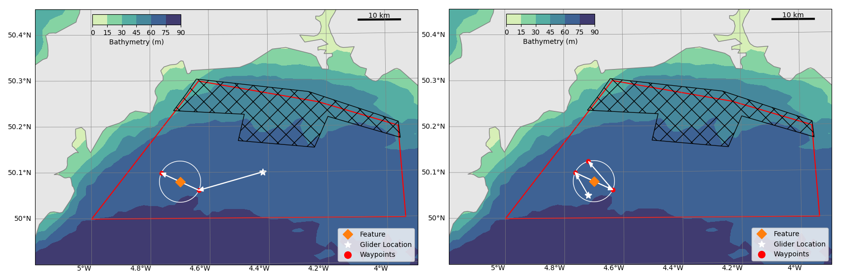
Figure 2 Path planning scenarios for a feature of interest (diamond). A 5 km radius circle drawn around the feature, if the glider is currently outside the circle waypoints are set to navigate to the circle boundary and transect across (left). If inside, systematically cover the circled region (right). Hatched areas are too shallow to safely operate the gliders, dashed red line used as a boundary for path planning.

The boundary of the glider operational region is marked in Fig. 2 with a solid red line, with the hatched region at the northern part of the operational region the typical no-go shallow zone for the class of gliders. To account for tidal advection pushing the gliders off course, a broad 5 km buffer zone is also applied around the edges for safety, as indicated by dashed red line.

From the probabilistic model, the location of a feature of interest is identified in the forecast period (e.g. maximum chlorophyll a, minimum dissolved oxygen or maximum uncertainty). A 5 km radius circle is created with the location as its center. The intention here is that the glider performs a transect along the direction of the dominant gradient of the feature within the identified circle.

If the initial location of the glider is outside the feature circle, the waypoints for the glider transect path are determined as follows: First, the dominant gradient path across the circle through the feature is calculated. Then the locations where this path crosses the circle are identified, with the closest point to the gliders current location used as the first waypoint. Lastly, the waypoints are set so that the glider proceeds along the dominant gradient path across the circle, as shown in the left subplot of Fig. 2.

Conversely, if the initial location of the glider is already inside the feature circle, waypoints are instead set to transect back and forth within the circle along the dominant gradient. When the glider path reaches the circumference of the circle, the dominant gradient is reversed and offset by a small angle to maximize are coverage, as depicted in the right subplot of Fig. 2.

2.5 Daily cycling during the field campaign

The operational window for the glider mission occurred in August–September 2024. During the operational glider deployment, the forecasting model was run daily at 08:30 UTC. An analysis step with data assimilation was run for the previous day, following which the model ran forwards without assimilation for 3 d to provide a forecast for 2 d ahead. Model outputs were post-processed to give values at fixed depths (z-levels) for chlorophyll and dissolved oxygen in the region around the glider deployment area (dashed line in Fig. 1), which were then passed to the probabilistic and path planning models by 13:00 UTC. The path-planning model produced waypoints by 16:00 for each glider for the following 24–48 h. These waypoints underwent human pilot checks for approval to ensure maritime safety before being transmitted via iridium satellite to the gliders while they were held at the sea surface. Glider data and satellite data were collected and provided to the model the following day and the cycle repeated.

2.6 Mission Summary

The mission provided numerous operational challenges. For the gliders this included occasional technical and communication failures, as well as some more critical vehicle and sensor issues which prompted a number of recovery and redeployment cycles. Unit 482 suffered a critical fault after two weeks and was not redeployed after recovery on 21 August 2024. Units 480 and 481 continued to operate until 30 August 2024, after which the campaign relied solely on Unit 480. This glider was recovered on 14 September for recharging and maintenance and was redeployed on 18 September alongside unit 481, both of which remained operational until the end of the observational campaign on 28 September 2024.

The operational area, shown by the red bounding box in Figs. 1 and 2, posed additional challenges. Shallow depths limited the available region and strong currents resulted in gliders occasionally moving outside the designated area. This was mitigated in part by the use of onboard thrusters controlled by remote human operators.

In total, glider observations were successfully obtained on 49 out of 54 d (6 August–28 September 2024), providing 90 % mission coverage. Of these, 15 d (28 %) included all three gliders operating simultaneously, 21 d (39 %) involved two gliders, and 13 d (24 %) had a single glider in operation. Only 5 d (9 %) were without glider activity.

The numerical simulations also featured many challenges. Communication failures occasionally meant simulations ran without the latest observational data. Additionally the simulations were performed on research infrastructure where the availability of computational resources was a limiting factor resulting in a delay producing the forecast data.

Figure 3 Mission Summary of glider deployment and path planning strategies used.

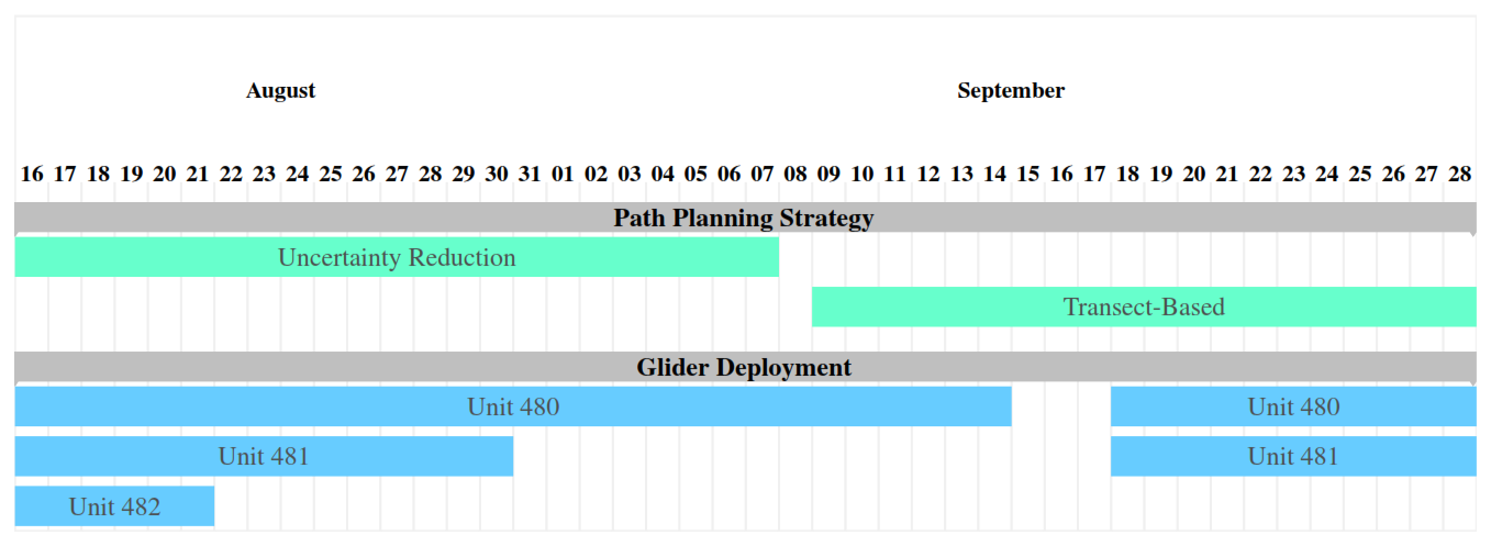
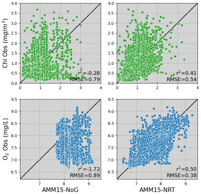
Figure 4 Glider observations of Chlorophyll a (top) and Oxygen (bottom) versus model predictions with no glider assimilation (left) and with (right).

Development of the probabilistic forecast and path planning system meant the system was not active at the start of the mission, first entering operation on the 16 August. Delays in receiving the forecast data or other computational issues resulted in some days when no new waypoints were generated. In that scenario the gliders were instructed to repeat the previous day's waypoints to maintain continuous operation. We implemented the first path planning strategy, focused on uncertainty reduction, from 16 August to 7 September, and then switched to the second, transect-based approach from 9 until 24 September.

During the mission period a Karenia bloom was observed via satellite in the Celtic Sea, but it did not migrate into the English Channel (Shutler et al., 2012). The glider network therefore had no opportunity to navigate to and measure the bloom over the operational period.

Despite these challenges, there were several periods where the entire DTO system was fully operational without human intervention, outside of standard monitoring and quality assurance.

3 Post-Mission Analysis

After the mission, a review of the various components of the DTO was carried out, with a series of additional simulations performed to focus on the impact that multiple co-ordinated gliders can have on the ability of the system to forecast observed conditions, or what might be considered the accuracy of the virtual twin. Assessment includes consideration of how increased resolution in the numerical model captures natural variability and features that are less well resolved in lower resolution, along with estimates for how the path planning component differs when the glider observations are not assimilated.

3.1 Experiments

As part of the post-mission analysis a series of experiments have been designed to explore the impact of observation processing and model resolution on the performance of the DTO. In total 4 simulations have been performed and will be reviewed in this paper:

• AMM15-NRT – Experiment on the 1.5 km grid assimilating near real time (NRT) SST and Chlorophyll a, along with NRT glider profiles of Temperature, Salinity, Chlorophyll a and Oxygen. This run is identical to the one that ran operationally during the mission, with none of the issues that occurred in real-time.

• AMM15-NoG – Experiment assimilating NRT SST and Chlorophyll a observations, akin to the current operational system but without assimilation of glider data.

• AMM15-DT – Experiment assimilating the same observational datasets as AMM15-NRT, with Chlorophyll a satellite data and glider profiles undergoing additional post-processing (aka delayed time (DT) observations).

• AMM7-NRT – Experiment using the same observations as AMM15-NRT on the lower resolution AMM7 domain.

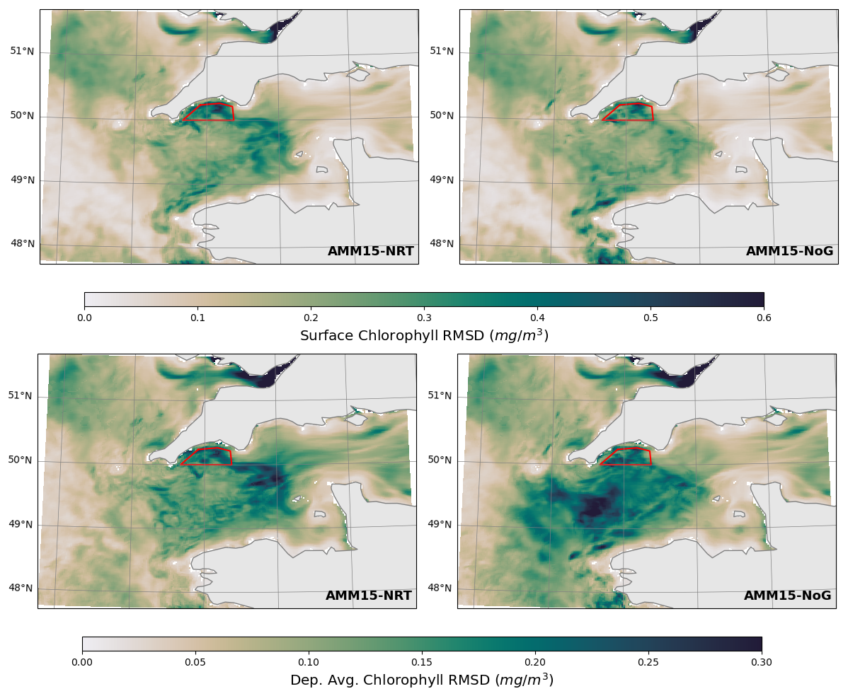
Figure 5 Time-averaged RMSD of the analysis fields for AMM15-NRT (left) and AMM15-NoG (right) against the AMM15-DT simulation across the simulation period for surface only (top) and water column averaged (bottom) fields. The glider operating area is indicated by the red box.

3.2 Impact of Gliders

Ford et al. (2022) demonstrated that assimilating glider observations can have a large impact on model forecasts of chlorophyll. Figure 4 shows the correlation between model and observation for the AMM15-NoG and AMM15-NRT experiments. Here the improvement from assimilating glider chlorophyll measurements results in a 32 % reduction in RMSE and an improvement in the correlation. For O₂ the improvements are even greater, with a 57 % reduction in RMSE. This is due to the gliders representing the only source of oxygen measurements assimilated in the system.

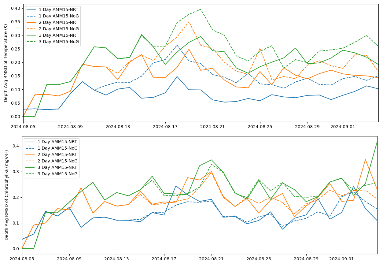
Figure 6 Spatially-averaged RMSD of forecasts from AMM15-NRT (solid lines) and AMM15-NoG (dashed lines) against the AMM15-DT analysis at different forecast lengths. Top – average water column temperature, bottom – average water column chlorophyll a.

In the absence of independent measurements we assume that the delayed time observations are the optimal observations and data assimilation improves model predictions, making AMM15-DT (as defined in Sect. 3.1) the best possible representation of the ocean state available. Figure 5 shows the model-to-model root mean square deviation (RMSD) for the other two AMM15 simulations [AMM15-NoG and AMM15-NRT] against the delayed time run for chlorophyll a. At the surface, the RMSD shows similar differences between the simulation using NRT data and the run with no gliders. This is likely due to the surface in the simulation being primarily impacted by satellite data, the assimilation of which was identical in both AMM15-NRT and AMM15-NoG. However, the impact of the gliders is shown to be significantly higher in results averaged over the entire water column, with large differences evident where no glider data has been assimilated. Despite a relatively small operating area (red box), the glider impact covers a large distance, particularly to the south west of the zone. For the NRT run, the difference is comparable to the surface RMSD, indicating that the impact of using delayed time gliders over near real time is smaller than the impact of using delayed time satellite data over near real time satellite data.

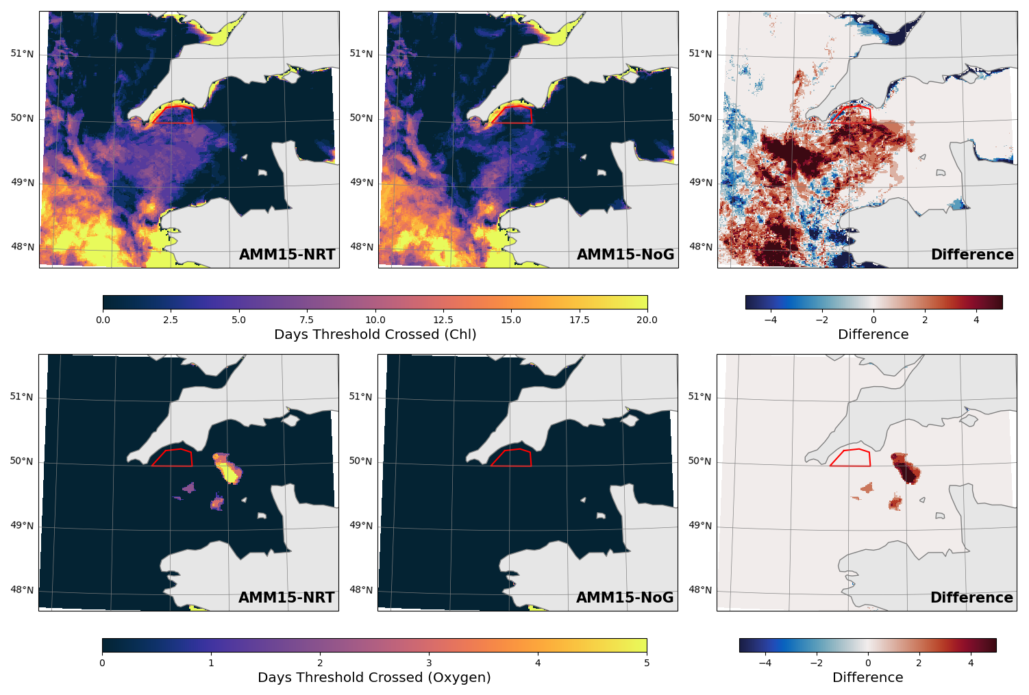
Figure 7 Instances the event state threshold is crossed anywhere in the water column for chlorophyll a (top) and oxygen (bottom) for the AMM15-NRT (left), AMM15-NoG (middle) and the difference between them (right).

A large element of the digital twin is the ability to produce informative forecasts to guide the path planning element. One approach to assess the forecast performance is to compare them at different lead times against the analysis solution. Figure 6 shows the RMSD of the day 1, 2 and 3 forecasts from the AMM15-NoG and AMM15-NRT simulations against the AMM15-DT analysis solution. For temperature, after a week from when the gliders start collecting data the difference without gliders at 1 d lead time is greater than near real time gliders at 2 d and similar to NRT 3 d ahead. For chlorophyll there is minimal difference between the two simulations, which suggests that averaged over a spatial region the size of the difference between processing levels is of a similar scale to the difference between including and excluding gliders. At 3 d lead time the difference to the analysis is around double that of the 1 d lead time, implying that without continual assimilation the model will drift away from the true state.

As part of the mission plan the gliders are targeting so-called “event states”, thresholds which indicate a feature of interest has developed. The thresholds are defined to be greater than 2.5 mg m⁻³ for chlorophyll (a typical bloom indication level), and below 6 mg L⁻¹ for oxygen (based upon OSPAR thresholds for the north west European shelf). Figure 7 shows the number of days the threshold is reached over the mission period between simulations with and without glider assimilation. For Chlorophyll a the event state is triggered significantly more to the south west of the domain, consistent with the changes shown with the assimilation previously. Inside the operational zone the event state would trigger on 2–3 extra occasions when glider data is assimilated. With dissolved oxygen, there is a notable increase in hypoxic events in the English Channel that were not identifiable without gliders, although within the operational zone there were no events.

3.3 Impact of Resolution

Comparison of the AMM15-NRT 1.5 km and AMM7-NRT 7 km resolution models reveal that there is a truly substantial impact of model spatial resolution (and the associated changes) on the inputs for the glider path planning. Whilst the two resolution models are not like-for-like prohibiting a full direct comparison, the two resolution models show large differences in the two essential biogeochemistry variables provided for the glider, chlorophyll a and dissolved oxygen (Fig. 8). Some of this can be attributed to a difference in initial conditions, particularly for bottom dissolved oxygen where the differences are consistently large across the domain and the forecast lead time. In this case the glider oxygen assimilation is seen to have limited impact in bringing the different resolution models closer together. In case of surface chlorophyll a, the model differences are substantially reduced in the analysis by the assimilation of the abundant satellite data, as well as the gliders, but those differences quickly grow in the model forecast highlighting the significance of grid resolution.

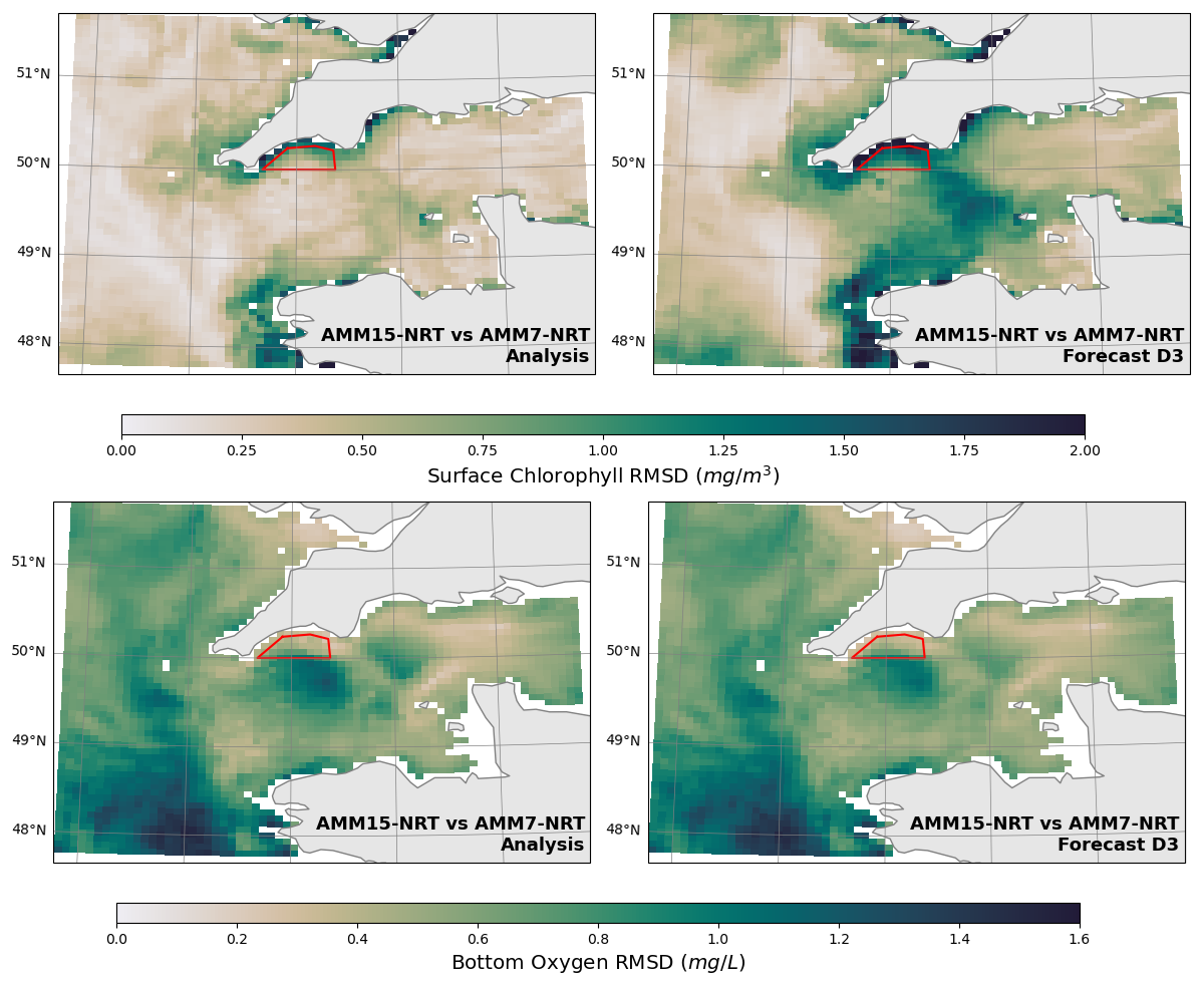
Figure 8 Time-averaged RMSD of the 1.5 km resolution and 7 km resolution model total surface chlorophyll a in mg m⁻³ (top) and bottom dissolved oxygen in mmol m⁻³ (bottom) for the analysis (left) and at 3 d lead time (right). As in the previous Figure, the 1.5 km model has been upscaled to the 7 km model grid.

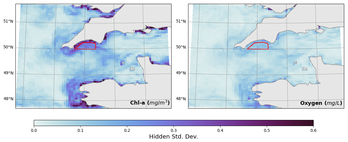
Figure 9 Variability represented by the 1.5 km resolution model, but hidden (averaged out) on the 7 km resolution model scale. The plots show the time-averaged third forecast day standard deviation for chlorophyll a (in mg m⁻³, left-hand panel) and bottom dissolved oxygen (in mg L⁻¹, right-hand panel).

The differences shown in Fig. 8 arise due to dynamical impact of the higher (1.5 km) spatial resolution on the biogeochemistry, as perceived on the 7 km scale. There is however additional benefit of the 1.5 km resolution model that comes from providing outputs at the finer 1.5 km spatial scale. This is assessed by Fig. 9 showing the 1.5 km spatial scale variability of chlorophyll a and dissolved oxygen that is unresolved at the 7 km scale. This variability is considerable especially for chlorophyll, but is smaller than the differences between the two resolution models at 7 km scale. For example the 1.5 km model at its resolution scale has a wider range of dissolved oxygen values, (4.5–13 mg L⁻¹), compared to the 7 km model (6.2–9 mg L⁻¹). However even after upscaling the 1.5 km model oxygen outputs to the 7 km scale, the interval of oxygen values remains almost as wide as on the 1.5 km scale (5.12–12.5 mg L⁻¹), and much wider than in the 7 km resolution model. In each case the 1.5 km model includes cases of moderate hypoxia (4–6 mg L⁻¹), whilst the 7 km model did not see hypoxia at all. Not surprisingly, the 7 km scale differences between the two resolution models, as well as the unresolved variability of the 1.5 km resolution model, are the greatest in the coastal areas (Figs. 8–9), where fine spatial resolution matters most.

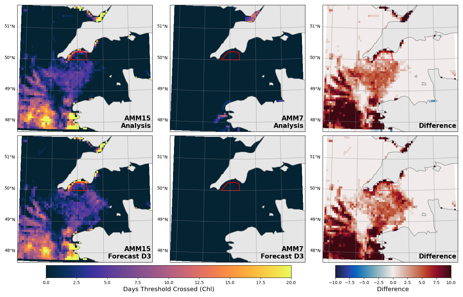
Figure 10 Number of mission days on which chlorophyll a concentration crossed the 2.5 mg m⁻³ threshold (anywhere in the water-column) on the 7 km spatial scale in the two models: (i) the 1.5 km resolution model in the left-hand panel, and the (ii) 7 km resolution model in the right-hand panel. The 1.5 km resolution model data have been upscaled to the 7 km model grid before the number of days was calculated.

The impact of the model differences on the glider path planning can be understood from Figs. 10 and 11. Unlike the 1.5 km model where the threshold for high chlorophyll a values is met on a big part of the domain including the glider area, in the 7 km model it is crossed only in very limited locations at the analysis time and in the next day's forecast. When it comes to dissolved oxygen, hypoxic events could be seen on a range of days in the coastal areas and western English Channel (including within the glider operation area) in the 1.5 km model, but the hypoxia threshold of 6 mg L⁻¹ was never crossed within the 7 km resolution model.

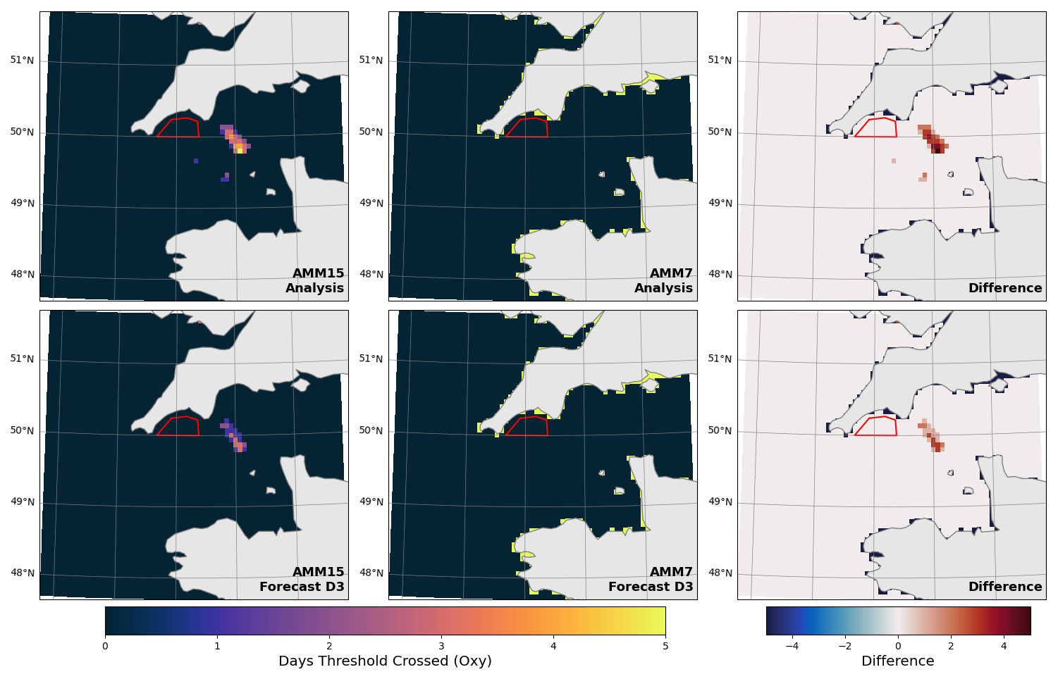
Figure 11 Number of mission days on which dissolved oxygen concentration crossed the 6 mg L⁻¹ threshold (anywhere in the water-column) on 7 km spatial scale in the two models: (i) the 1.5 km resolution model in the left-hand panel, and (ii) the 7 km resolution model in the right-hand panel. The 1.5 km resolution model data have been upscaled to the 7 km model grid before the number of days was calculated.

3.4 Impact of Gliders on Path Planning

As part of the post-mission reanalyses the probabilistic forecast and transect based path planning has been run using outputs from both AMM15-NRT and AMM15-NoG for comparison. The run sets paths for two gliders, with one targeting maximum chlorophyll and the other minimum oxygen. As this is being performed post-mission the paths will be decoupled from the actual gliders that provided measurements for the assimilation.

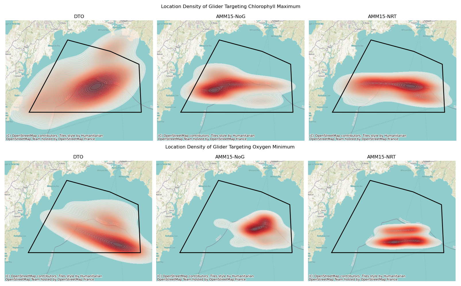
Figure 12 Heatmaps of glider locations over the mission period for the real digital twin (left), theoretical path from AMM15-NoG simulation (middle) and theoretical path from the AMM15-NRT simulation (right), for the glider targeting maximum chlorophyll (top) and minimum oxygen (bottom). ting time. Left – glider targeting maximum chlorophyll, Right – glider targeting minimum oxygen. Bottom – Hypothetical distance between glider waypoints

The location density of where the gliders operated during the mission, or would theoretically operate using the post mission model output, are shown in Fig. 12. The glider targeting chlorophyll covered a large portion of the mission area, travelling back and forth across the zone, no matter the simulation used, which suggests high uncertainty with regards to the maximum chlorophyll location, or the presence of multiple local maxima in the area. In the absence of feedback from the glider measurements, the glider would have spent the most time in the west of the domain, compared with the reality more towards the east. The distance between density centers of the heatmaps for the DTO and the AMM15-NoG simulation is around 35 km, with distances over time ranging between 3 and 50 km as the gliders traverse back and forth. This results in a glider that could be operating over a day of travel away from the target zone, potentially missing localised events.

For oxygen, the dynamics tend to be much slower moving compared to chlorophyll with the gliders in all cases identifying an oxygen minimum zone in the south east of the domain. Without feedback of the glider observations the paths planned with the AMM15-NoG data put the glider further north in the center of the domain. The use of the transect based strategy for the whole period is clearly evident in the AMM15-NRT paths, with the glider travelling east-west along the boundary of the operational zone. Whilst the distance between the density centers is much smaller for the oxygen targeting glider, there is a consistent distance between the gliders of around 16 km, caused by shift in the simulated location of the oxygen minimum when glider observations are included. Operationally, slow moving features can lead to the glider sitting around a small area for the majority of a mission which may not be the optimal use of the equipment. A revised strategy may be worth considering depending on the goals of the mission.

4 Conclusions

This paper has presented an exciting Digital Twin Ocean framework that enables a continual two-way coupling between real and virtual environmental systems via a continuous feedback loop of measure, predict, direct and refine. Building on a pilot study of Ford et al. (2022), every element of the digital twin has evolved to optimise the overall impact of the system.

We show that the inclusion of multiple in-situ glider observations within higher resolution models significantly improves the data assimilation product and subsequently the predictive skill of the model. This extends beyond immediate reduction of bias/error at the time of assimilation to recognisable improvement over the short-term forecast period. Instances where the forecast predicts the crossing of key thresholds in both chlorophyll and dissolved oxygen also increase with the inclusion of these glider measurements, resulting in a system that captures extremes more readily and accurately.

The numerical model used in this study also benefits from increased resolution compared to previous work (Ford et al., 2022), capturing features that would have previously been missed at the current UK operational resolution. In the current operational system much of the natural variability in the system is lost, especially close to the coast. Additionally, several instances of the key threshold for chlorophyll are identified that were otherwise missed, whilst some dissolved oxygen events are predicted that are missed entirely at the lower resolution.

The two-way coupling and path planning algorithm provided valuable improvements to navigation of the gliders, locating and better resolving target events as they evolve. Using multiple gliders has also proven to be a major asset, as the oxygen minima were largely misaligned with the chlorophyll maxima (or other key features), so they could not both be captured by the same single glider.

Assimilating delayed mode data was also shown to improve the results from simulations with near real time observations, with an impact on glider navigation. Any future mission could substantially benefit from speeding up the data processing in real time to make use of these observations.

The DTO system provides many exciting opportunities for the future, including: (i) addressing challenges with combining in-situ measurements alongside satellite fields within data assimilation through cross-calibration and bias correction, (ii) accounting for the multi-scale issues in estimating error covariance matrices and representativeness errors, making use of diagnostics such as Fowler et al. (2023), (iii) adding automatic imaging cameras to the gliders to better distinguish phytoplankton species and (iv) using ML to speed up prediction and derive addition information, such as the likelihood a chlorophyll bloom is due to Karenia mikimotoi.

This work represents a major advance in our ability to deploy a true Digital Twin Ocean, that not only improves model outputs through the ingestion and assimilation of observational data, but that optimises both the predictive capability of the virtual twin, while improving the effectiveness of the real-world monitoring strategy. This framework has immediate value to those requiring near real-time understanding of complex environmental systems for improved management and early warning systems.