Modulation of internal tides properties off the Vitória–Trindade ridge during contrasted seasons from altimetry and a regional ocean model

The incoherent fraction of internal tides, generated through interactions with mesoscale eddies and other transient oceanic features, remains poorly understood and challenging to predict. This limits our ability to accurately represent energy transfers and mixing induced by these waves. The Vitória–Trindade Ridge off the Brazilian shelf is a relevant natural laboratory to investigate these processes, as a hotspot for internal tides generation embedded in a region of intense mesoscale activity. To assess how seasonal stratification and mesoscale variability modulate internal tides, we compared a 27-year satellite altimetry record with a high-resolution ($\mathrm{1}/\mathrm{36}\mathit{°}$) regional simulation using NEMO v4.0.2. This joint analysis allows us to characterize the generation, propagation, and dissipation of internal tides under two contrasted regimes: austral winter (defined here from May to October) marked by a deep pycnocline, and austral summer (defined here from November to April) with a shallower and sharper seasonal pycnocline. Both model and observations depict six intense, in-phase beams of the baroclinic flux propagating southward from the ridge. The first two have a wavelength of 100 km approximately corresponding to the mode-1 of propagation, while more distant beams are spaced by about 50 km only, which likely corresponds to the mode-2 of propagation. Quantification from the model shows that generation rates are 5 %–15 % higher in summer than in winter. Dissipation occurs predominantly near the ridge (45 %) but also extends offshore (40 %), reaching beyond 2–3 mode-1 wavelengths. In the open ocean, dissipation is up to 40 % stronger in winter, leading to a weaker baroclinic flux propagating on shorter distances compared to summer. Altimetry confirms seasonal variations in both wavelength and amplitude, especially for mode-2 internal tides. Finally, a representative case of interaction between internal tides and a mesoscale eddy is documented under summer conditions, showing deviation and diffraction of the baroclinic flux. This study demonstrates that mesoscale variability and seasonal stratification jointly modulate the coherence and energy pathways of internal tides. These findings are essential for improving predictions of the incoherent tide and for interpreting high-resolution altimetric observations.

1 Introduction

As part of the Earth climate system, the ocean is playing a major role in the regulation of climate. With the increase of greenhouse gases in the atmosphere, the energy budget of the Earth is nowadays unbalanced. According to the Intergovernmental Panel on Climate Change, the ocean is absorbing up to 90 % of the energy emitted by human activities (IPCC, 2023). The absorption of this energy is happening through oceanic processes of various scales, from the global ocean circulation to turbulent mixing that enables exchanges of heat, salts, nutrients, pollutants, and sediments between the vertical layers of different densities in the ocean (Ferrari and Wunsch, 2009). In particular, internal tides have been identified as one of the main drivers for diapycnal mixing (Garrett, 2003; Arbic et al., 2018). These internal waves forced at the tidal frequency are usually called baroclinic tides. They induce vertical displacements of the order of hundred metres within the water column and occur when the barotropic tide pushes the stratified water column over a topographic obstacle, like a ridge or a continental slope (Gerkema and Zimmerman, 2008). Baroclinic tides have been identified as a major cause of the dissipation of the barotropic tide (Nugroho et al., 2018; Shakespeare, 2019). It has been estimated in the past that 1 TW out of 3.5 TW of the barotropic energy is converted into baroclinic energy (Egbert and Ray, 2001). Thus, internal tides transfer energy from climate scale to meso- to submesoscale. Their role in the ocean energy cascade is currently investigated as a hot topic in oceanography in order to improve climate monitoring and forecasting (Whalen et al., 2020).

Nonetheless, the mechanisms of internal tides remain difficult to unveil due to their non-linear dynamics, their spatio-temporal scales and their medium of propagation. Internal tides are characterised by a wavelength ranging from a few to a hundred metres, and propagate over a few hours to a few days (Wunsch, 1975). They can be observed by measuring their mixing contribution to turbulent processes in the water column, thanks to in situ instruments such as Acoustic Doppler Current Profiler (Subeesh et al., 2021; Löb et al., 2020; Fernández-Castro et al., 2020). However in situ data remain costly and scarce. To ensure a broader coverage of the global ocean, satellite remote sensing has been developed over the last decades. With Synthetic Aperture Radar (SAR) imagery, optic images and above all altimetry, the surface signature of internal waves can be detected by the elevation of the sea level of few centimetres (Carrère et al., 2004; Klemas, 2012; Ansong et al., 2017). Indeed satellite data can only provide information on the surface of the ocean, while the main internal tide signal is usually located around the pycnocline. In December 2022, the launch of the Surface Water and Ocean Topography (SWOT) satellite and its revolutionary Ka-band radar interferometer (KaRIn) technology provides bi-dimensional Sea Surface Height (SSH) observations at finer scales (5–200 km), which were never reached before by nadir altimetry (Morrow et al., 2018). The SWOT 21 d repeat orbit allows a complete mapping of the global ocean using two swaths located 60 km apart along the satellite track, with a horizontal resolution of 2 km and SSH errors less than 4 mm (Fu et al., 2024). Hence, the surface signature of internal tides is better captured by SWOT than conventional altimeters. This may complicate the analysis of high-resolution SSH observations (Carrere et al., 2021). A thorough understanding of internal tides variability may therefore help interpret this new type of data.

In this article, we focus on the internal tides variability off the Vitória-Trindade Ridge (VTR), over which SWOT passed every day during its calibration phase. This study is meant to bring some insights on the region dynamics for a better interpretation of the first SWOT data. Internal tides in the South Atlantic have not been documented as much as in other ocean basins until recently. The VTR is composed by a succession of seamounts around 20.5° S extending from the Abrolhos bank to the Trindade island and has been identified as a main generation site for internal tides (see Fig. 1). By using altimetry data, Paiva et al. (2018) showed that the baroclinic tides were radiating away from the ridge, both southward and northward. Additionally, the arc shape of the VTR induces a lens effect on the south baroclinic flux. We restricted our analysis to the tide generated by the principal semidiurnal component M2, identified as the dominant one (Toffoli et al., 2023). The Brazilian Current (BC) is crossing the VTR while flowing southwards along the Brazilian coast. In the surface layers, BC transports warm and salty waters originating from the South-Equatorial Current (SEC), while Intermediate Western Boundary Current (IWBC) carries underneath dense and cold waters, coming from higher latitude and propagating in the opposite direction (Napolitano et al., 2021). Due to the interactions of these main currents with the steep topography of the VTR, mesoscale eddies are generated on either side of the ridge: the counter-clockwise anticyclonic Abrolhos Eddy north of the ridge and the clockwise cyclonic Vitoria eddy south of the ridge and the Abrolhos Bank. These eddies are creating instabilities and meanders in the region, enhancing a turbulent background circulation around the VTR (Dossa et al., 2022). The regional geography and ocean dynamics are summarised in Fig. 1.

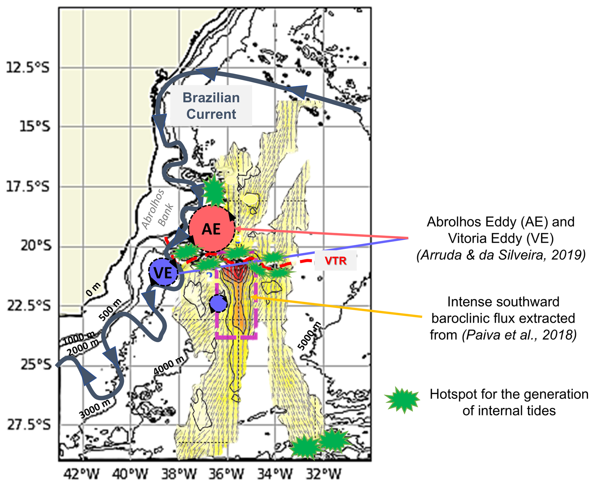
Figure 1 Scheme of the regional ocean dynamics around the VTR. The bathymetry is steep, with seamounts reaching the first 50 m of the water column. The Brazilian current is crossing the VTR and two stationary eddies are on either side of the VTR: the Abrolhos eddy and the Vitoria eddy, from which some smaller eddies are detaching. The background circulation appears quite turbulent. The baroclinic flux represented in this Figure was extracted from Paiva et al. (2018) but will be retrieved in this study with our own tools. It appears that internal tides are more intense south of the VTR. Green stars indicate hotspots for the generation of internal tides in the area.

Located at subtropical latitudes, the VTR appears as an ideal case study to characterise the variability of internal tides – from their generation to their dissipation – and their possible interactions with mesoscale processes. Here, we propose to analyse the internal tides not only through the spectrum of nadir altimetry measurements but also using an hydrodynamical model at a $\mathrm{1}/\mathrm{36}\mathit{°}$ resolution. The resulting numerical simulations offer a complete description of the whole water column of the ocean dynamics with a horizontal resolution of the order of 3 km over the model domain.

In this work, we first introduce the altimetric data and the high-resolution numerical model named TAPIOCA-36. We provide preliminary results on the internal tides general properties. Secondly, we analyse the seasonal variability of the region and describe how it impacts the generation, propagation and dissipation of internal tides. Finally, we present a qualitative case study of an eddy-internal tides interaction.

2 Data

In order to analyse the variability of the baroclinic tide over the VTR, we use two different tools: conventional nadir altimetry data and numerical modeling. In this section, the altimetric data processing steps and the regional high-resolution model – TAPIOCA-36 – are presented.

2.1 Altimetry

For this study, all available satellite tracks of the TOPEX/Poseidon and Jason-1/Jason-2/Jason-3 missions are considered. We chose these satellite missions since they form together a time series of data from 1993 to 2025 with a revisit period of 9.9156 d. We select data from 1993 to 2020 to conduct a harmonic analysis. While tidal frequencies remain aliased due to the satellite sampling pattern, the length of our time series enables a reliable disentangling of the various tidal components, even when separating the data into two contrasted seasonal periods (Ubelmann et al., 2022).

In order to retrieve the internal tides' signal on the region, the following processing steps have been applied (Carrère et al., 2004):

1. Step 1: We conduct an harmonic analysis on the along-track Sea Level Anomaly (SLA) retrieved at each pass of the nadir altimeter according to the decomposition: $h(x,t)=h_{\mathrm{0}}\left(x\right)+h_T(x,t)+\mathit{ϵ}(x,t)$ where h is the Sea Surface Height (SSH) measured at the location x and time t, h₀ is the mean SSH of the ocean at location x, ϵ is the residual signal including the non-coherent part of the baroclinic tides. h_T is the contribution of barotropic and coherent baroclinic tides to the SSH: $h_T(x,t)={\sum }_{i=\mathrm{1}}^N{A}_i\left(x\right)\cos ({\mathit{\omega }}_{i}t+{\mathit{\varphi }}_i)$ where A_i is the amplitude, ω_i is the angular velocity, and ϕ_i is the phase of the $i\text{th}\in \left[\right|\mathrm{1},N\left|\right]$ wave at the location x and time t. We focus here on the M2 component, characterised by $\mathit{\omega }=\mathrm{1.405189}{\mathrm{s}}^{-\mathrm{1}}$. Hence, we recover the SSH linked to the M2 tidal frequency from altimetry.

2. Step 2: We apply a spatial filtering on the M2 component to separate the baroclinic from the barotropic tides. We use a Lanczos low-pass filter with a cut-off wavenumber at $\mathrm{1}/\mathrm{500}$ km⁻¹.

In this study, track 137 of the TOPEX/Poseidon – Jason 1/2/3 mission is used to analyse the internal tide signal in the SSH. Hence, we use all other tracks of the mission crossing the track 137 to evaluate the uncertainty of the M2 baroclinic signal retrieved with our method. By computing the standard deviation of the differences in the M2 baroclinic amplitude at cross-over points, we estimate an uncertainty of about 0.3 cm, which represents a 10 % relative error on the amplitude.

We further evaluate the consistency of this processing method (Lanczos) with the High-Resolution Empirical Tide (HRET) model from Zaron (2019) for the baroclinic signal and with the FES2014 model for the barotropic signal (Lyard et al., 2021). Both of these models are based on altimetric data. While HRET targets the modeling of internal tides, FES2014 provides a reconstructed field of the SSH through the resolution of the tidal barotropic equations. Therefore, these two models are relevant to evaluate our processing method relying on a simple filtering of altimetric data only.

We focus on the latitudes south of 20° S since we will study further the baroclinic flux propagating southwards. We display the comparison results on the track 137 flying over the ridge around 36° W, where internal tides are known to be the most intense (Paiva et al., 2018) (see Fig. 2). We notice that the baroclinic signal retrieved by the Lanczos filtering is in reasonable agreement with the one derived in the HRET model, although the amplitudes appear slightly larger – sometimes with a difference of up to 30 %. While we process and keep nadir signal in this study, the HRET model produces a complete 2D map of the internal tides surface signature. It relies on the optimal interpolation of altimeters' nadir tracks. This method is known to smooth the overall signal, which may explain this slight difference in amplitude compared with our result (Chelton and Schlax, 2003). This difference could also be explained by some residual barotropic signal remaining in the baroclinic signal after applying the spatial filtering.

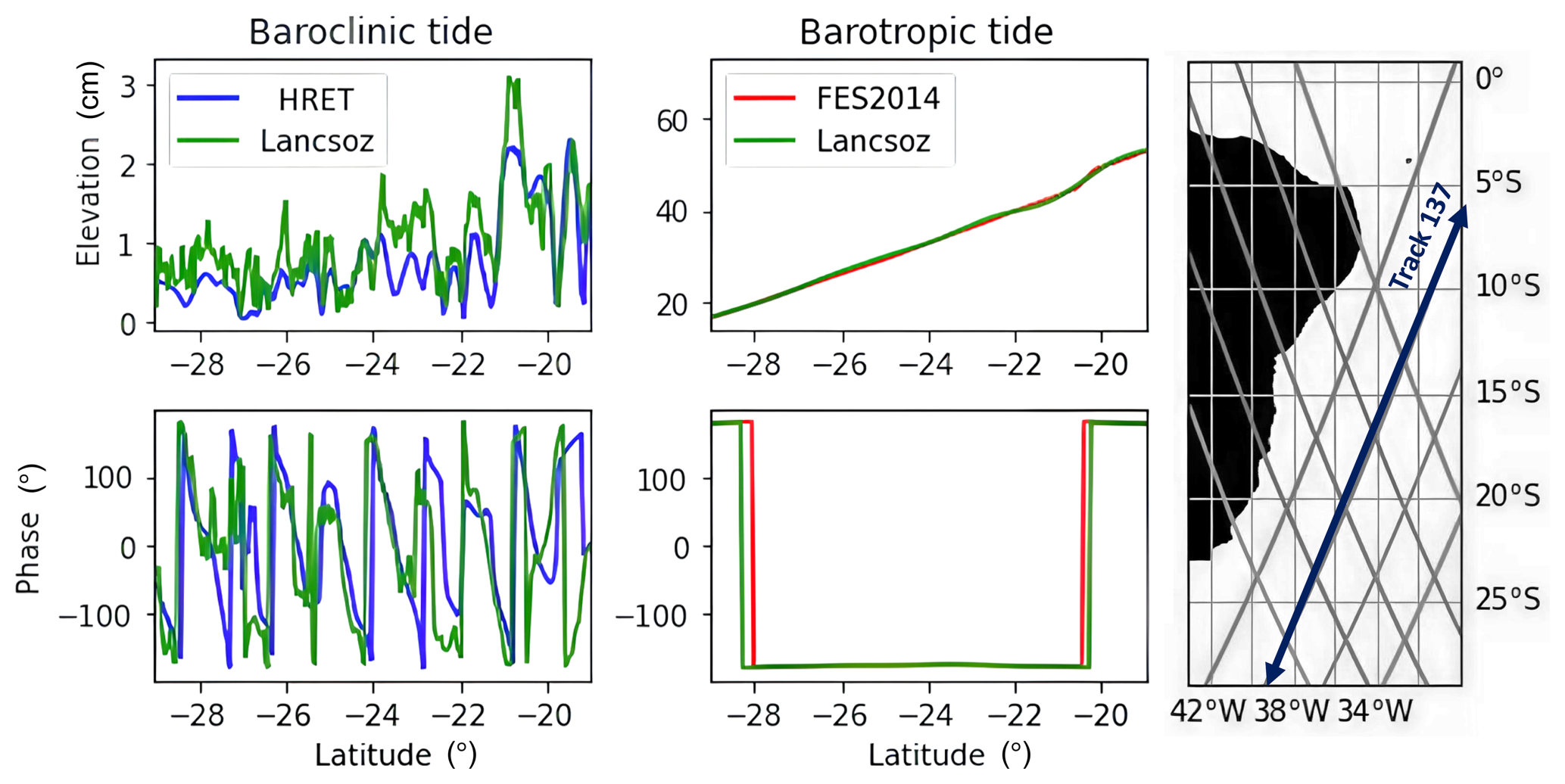
Figure 2 Comparison of the baroclinic and barotropic signals' elevation (upper row) and phase (lower row) extracted from the track 137 of the TOPEX/Poseidon mission following our processing steps with the HRET model and the FES2014 model. We note that the phase discontinuities should not be interpreted as strong physical variability but rather result from the convention chosen for the phase range. The map on the right displays every available track on our region of study from the TOPEX/Poseidon and Jason missions.

When we compare the barotropic signal retrieved from our spatial filtering (see Fig. 2), we recover a signal close to the FES2014 model, thereby validating our processing method. As for the phase of the baroclinic signal, it encounters an inversion at 21° S, near the VTR. This confirms a propagation of the baroclinic tides in two opposite directions. A slight phase delay is observed between the Lanczos method and the models, but our results remain consistent with the phenomenology of the area. In addition, this filtering method is simple and computationally cost-effective and still provides sufficiently accurate results. These characteristics motivated its use in this study.

2.2 A regional oceanic model: TAPIOCA-36

We use regional simulations based on the forced ocean hydrodynamical model NEMO4.0.2. (Nucleus for European Modelling of the Ocean), which provides high resolution data (Madec, 2017). This regional model is named hereafter TAPIOCA-36. It benefits from an horizontal resolution of $\mathrm{1}/\mathrm{36}\mathit{°}$ (∼3 km), and 75 fixed z coordinates levels ranging from 0 to 5000 m depth. The grid resolution is finer in the first 100 m of the water column, counting 23 levels, while the thickness of the deepest model-level reaches 160 m. This configuration should be able to capture submesoscale phenomena, like meanders, jets, eddies and low-mode internal tides evolving in the upper layers of the ocean. A third-order upstream based scheme (UP3) with built-in diffusion is also implemented for momentum advection. The k–ϵ turbulent closure scheme constrains the vertical diffusion coefficients. Bottom friction is quadratic with a bottom drag coefficient of 0.0025, while we assume lateral wall free-slip boundary conditions. The temporal integration is achieved by an Asselin filter with a time step of 150 s. The time-splitting technique used in NEMO4.0.2. resolves the internal tides signal as it uses smaller time steps for the computation of the barotropic tides velocities. In this configuration, initial conditions for oceanic velocity fields, SSH, temperature and salinity, as well as open boundary conditions at the edges of the model domain, are given by the global ocean assimilative eddy-permitting GLORYS12v1 reanalysis in order to represent realistically the ocean large scale circulation (Lellouche et al., 2018). For similar reasons the model is forced during its time-integration by the surface atmospheric fluxes of the ERA-5 reanalysis (Hersbach et al., 2020). Eventually, FES2014 has been applied on the open boundaries to force the direction, elevation and barotropic currents of the 15 primary tidal components (M2, S2, N2, K2, 2N2, MU2, NU2, L2, T2, K1, O1, Q1, P1, S1, and M4) (Lyard et al., 2021). We run the model over 2 years: 2008 is used for validation and 2009 for the rest of the study. For these two years, seasonal, monthly and daily outputs were computed for the following fields: temperature, salinity, SSH, oceanic horizontal and vertical velocities. An harmonic analysis is also computed on-line by the model to isolate and retrieve the 15 primary tidal frequencies, including M2. The method introduced by Kelly et al. (2010) is used to separate barotropic and baroclinic tide constituents. This separation is directly performed at each time step by the model during the simulation. The baroclinic energy flux F_bc (Eq. 1), the conversion C (Eq. 2) and dissipation D (Eq. 3) rates are then derived on-line, according to the following formulas:

$$\begin{array}{}\text{(1)}& {\displaystyle }& {\displaystyle }{F}_{\text{bc}}=\underset{-H}{\overset{\mathrm{0}}{\int }}\stackrel{\mathrm{‾}}{V_{\text{bc}}{p}_{\text{bc}}}\mathrm{d}z\left({\mathrm{m}}^{\mathrm{3}}{\mathrm{s}}^{-\mathrm{1}}\right)\text{(2)}& {\displaystyle }& {\displaystyle }C={\mathrm{\nabla }}_{z}H\stackrel{\mathrm{‾}}{V_{\text{bt}}{p}_{\text{bc}}}\left(\mathrm{W}{\mathrm{m}}^{-\mathrm{2}}\right)\text{(3)}& {\displaystyle }& {\displaystyle }D=C-\mathrm{\nabla }{F}_{\text{bc}}\left(\mathrm{W}{\mathrm{m}}^{-\mathrm{2}}\right)\end{array}$$

where H is the depth, V_bc is the baroclinic velocity, V_bt is the barotropic velocity, p_bc is the baroclinic pressure.

To validate TAPIOCA-36 tidal forcing, we compare the M2 tidal signal contribution with the SSH over the spin-up year 2008 to the one of FES2014 (Fig. 3). Figure 3 shows that the tidal amplitudes and phases are satisfactorily reproduced by TAPIOCA-36. The contribution of the M2 tidal frequency to the SSH of FES2014 refers only to the barotropic tide as a one-layer model, whereas TAPIOCA-36 merges both baroclinic and barotropic tides contributions by taking into account the stratification of the water column. It explains the stronger variability in the amplitude and phase of the tidal signal plotted for TAPIOCA-36. Subsequently, we validated qualitatively the stratification of TAPIOCA-36 against in situ data provided by the World Ocean Atlas (WOA) over the year 2008 (Levitus et al., 2010). We average every available temperature and salinity profiles within a box extending from 20.5 to 29° S in latitude and from 40 to 33° W in longitude (see Fig. 3). The mean temperature and salinity profiles of the first 500 m of the water column of TAPIOCA-36 show a good overall agreement with the ones reported by the WOA, although we note that TAPIOCA-36 is slightly saltier than the WOA data. This comparison provides a qualitative consistency check rather than a full validation of the model stratification. We refer the reader to Giachini Tosetto et al. (2024) for additional quantitative validation work of TAPIOCA-36 against ADCP data and GLORYS12v1 data.

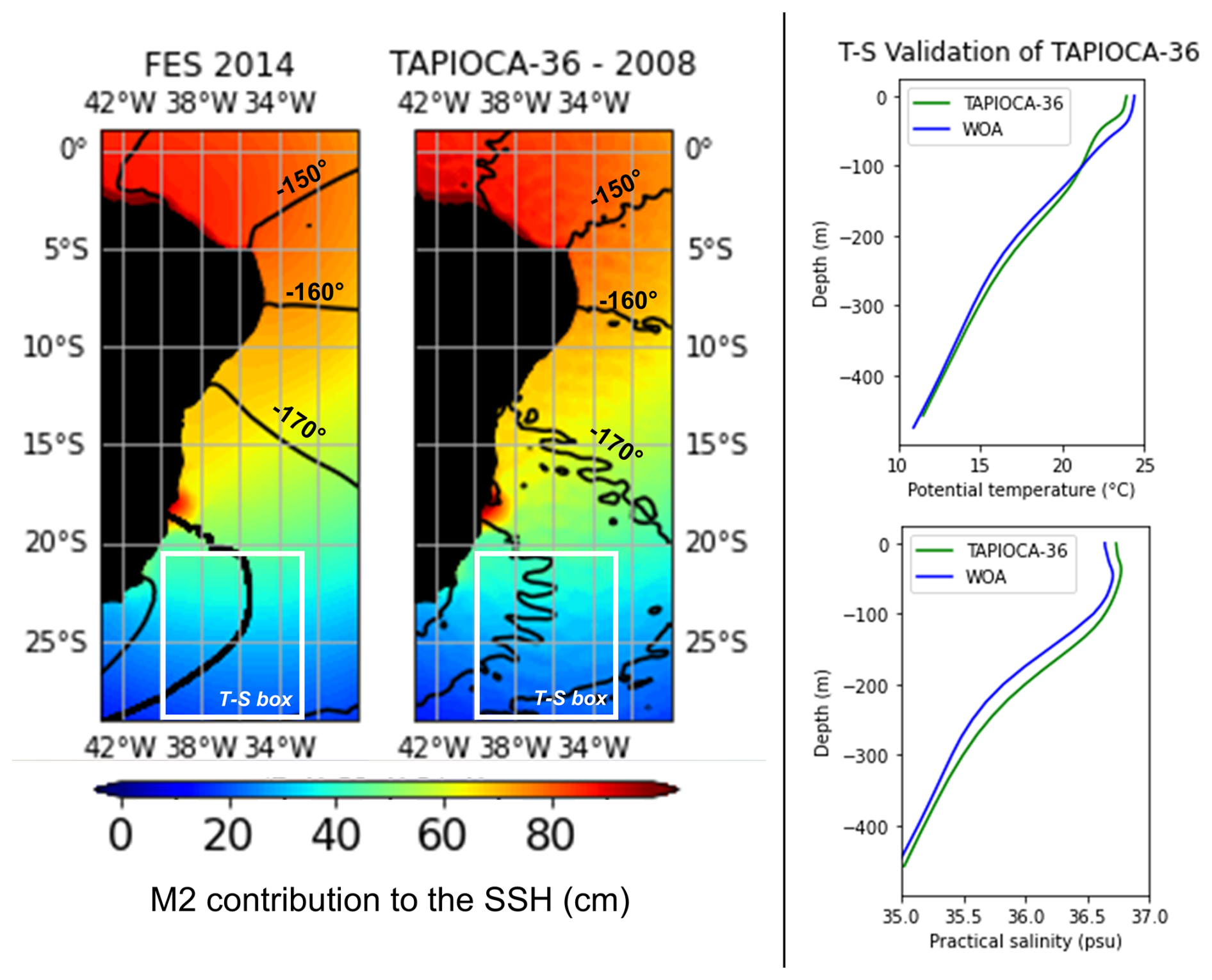
Figure 3 Left panel: Maps of the M2 tidal signal contribution to the SSH elevation in the FES2014 model (barotropic tide) and in TAPIOCA-36 simulation (including both barotropic and baroclinic tides). The tidal phase is represented by black contour lines. The white box delimits the area in which temperature and salinity profiles were selected for further validation. Right panel: Averaged Temperature and Salinity profiles of TAPIOCA-36 against WOA data in 2008.

3 Results

3.1 Internal tides general properties

We start with an overview of the internal tides' variability at the VTR. Altimetry and the TAPIOCA-36 simulation in 2009 provide complementary information to characterise the generation, the propagation and the dissipation of internal tides. On one hand, altimetry refers to internal tides which were actually observed over the past 27 years at the surface of the ocean. On the other hand, the TAPIOCA-36 product simulates internal tides using physical equations derived for this area. It therefore provides insights into the dynamics not only at the surface but throughout the water column.

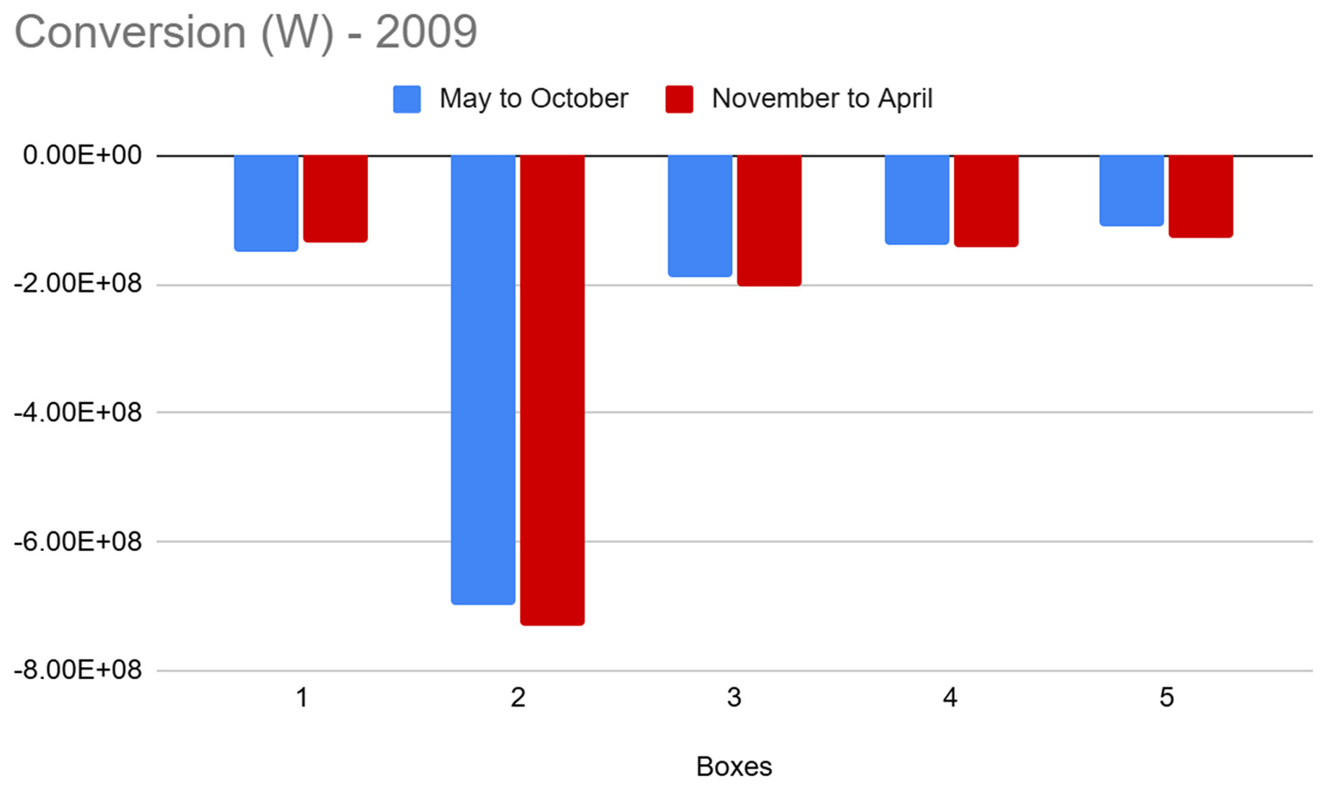
The VTR is identified as a major generation site for internal tides, with conversion rates from barotropic to baroclinic energy reaching up to $-\mathrm{0.3}\mathrm{W}{\mathrm{m}}^{-\mathrm{2}}$, according to the model (see Fig. 4). We note that the conversion from barotropic to baroclinic energy is not strictly negative in TAPIOCA-36. This does not mean that there is a transfer from baroclinic to barotropic energy, but rather indicates a phase shift between barotropic velocity and baroclinic pressure fields (see Eq. 2), as explained by Carter et al. (2008). We define 5 boxes surrounding the VTR for a finer local analysis and integrate the conversion rate within each box by summing the grid-cell conversion rates weighted by cell surface area. Conversion rates are expected to be the highest in box 3, as the VTR lens effect makes the energy converge at this location, following the study of Paiva et al. (2018). Our model quantitatively shows that box 3 accounts for nearly half of the conversion of barotropic energy into baroclinic energy. Moreover, the further away from box 3, the lower the conversion rate (see Fig. 4).

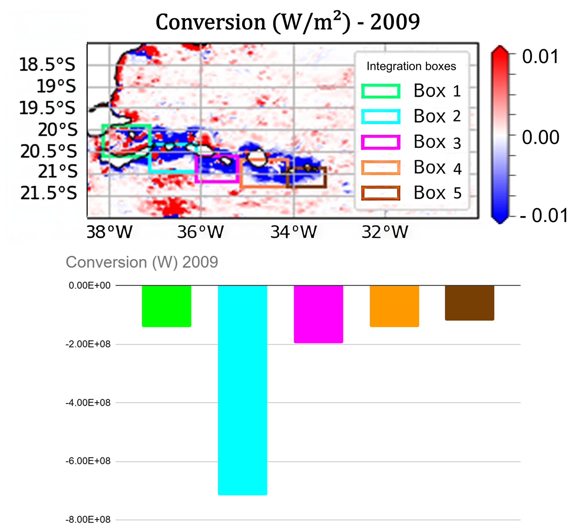
Figure 4 Upper panel: Map of conversion rates from barotropic to baroclinic energy in the VTR region during 2009 from the TAPIOCA-36 simulation. Lower panel: Conversion rates integrated in 5 boxes spread along the ridge.

After their generation, internal tides propagate away from the ridge, mostly southwards. We analyse their pattern of propagation and assess the consistency between the TAPIOCA-36 simulation and altimetry data along the track 137. To achieve this, we co-located the TAPIOCA-36 data with the trajectory followed by the satellite on track 137. In Fig. 5, we display the elevation of the SSH linked to the M2 baroclinic tide according to altimetry and our simulation. This comparison indicates that the baroclinic signal varies with the same order of magnitude both in the altimetric data and in the model, even though TAPIOCA-36 tends to amplify the signal, with a M2 baroclinic amplitude peak of 4 cm at the VTR (∼20.5° S) symbolised by a blue line on the Fig. 5. We notice that the altimetric signal is slightly offset from the TAPIOCA-36 simulation output. It is important to recall here that the harmonic analysis of altimetry has been conducted over 27 years of data, whereas the harmonic analysis of TAPIOCA-36 has been computed on one year only. Note that some holes remain in the TAPIOCA-36 product because of the presence of islands and seamounts. No interpolation has been applied to keep the baroclinic signal intact from any smoothing. At 22° S, the behavior of the model and of the altimetric data appear disparate as their baroclinic signals are not completely in phase anymore over a few hundreds of kilometres. In the next sections, we will see that interactions between internal tides and the background circulation are likely to happen at these latitudes and can alter the internal tides signature.

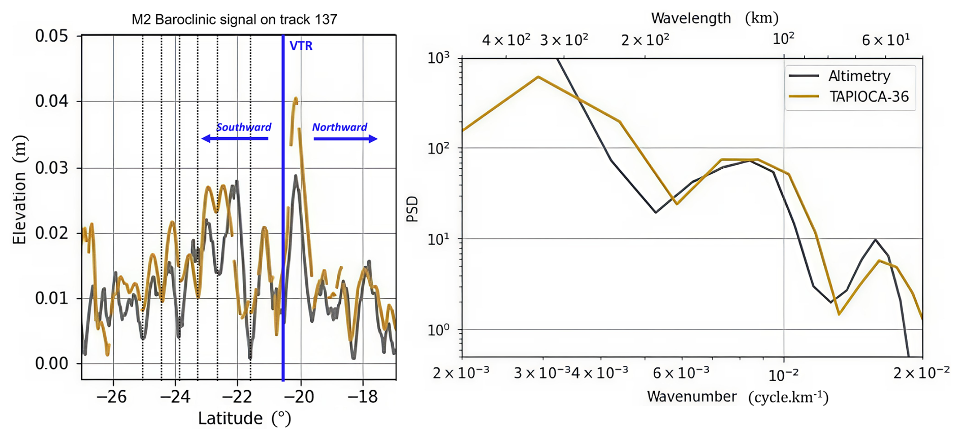
Figure 5 Left panel: Contribution of the M2 tidal component to the elevation of SSH in altimetry and in TAPIOCA-36 data. The blue line indicates the location of the VTR. The arrows indicate the direction of propagation of internal tides. The dotted lines identify the successive beams of reflection of internal tides. Right panel: Power spectrum of the M2 baroclinic signal in altimetry and in TAPIOCA-36 data.

Besides, the spectral analysis displayed in Fig. 5 shows that the first mode of propagation is the most energetic. More precisely, the spectrum indicates a wavelength of approximately 140 km. The second mode is also observable, with a wavelength of around 65 km. As the altimetric track crosses the internal tides flux at an angle of about 20°, the actual wavelengths of the first and second mode of propagation are respectively 131 and 61 km. Nonetheless, there is a slight difference of around 5 km between the altimetric and the TAPIOCA-36 signals. This difference remains acceptable and is in agreement with the study of Paiva et al. (2018).

Despite this variability in the baroclinic signal between altimetry and TAPIOCA-36, the reflection beams of the baroclinic signal captured by altimetry fit the ones of the model, hence supporting the consistency between our different datasets. A reflection beam refers to a beam of internal tide energy that results from the reflection of a primary beam on the surface in our case. After being reflected, this beam propagates away from the reflection point following the direction imposed by the internal wave dispersion relation. In our analysis, these reflection beams are identified as coherent structures in the SSH signal, corresponding to regions where baroclinic energy remains concentrated along preferential directions. In particular, the first reflection beam happens at around 100 km away from the ridge. It corresponds approximately to the order of magnitude of the wavelength of the first mode of propagation (right panel of Fig. 5). The second reflection beam also happens around 100 km away from the first beam. This indicates that the propagation of internal tides might be dominated by the first mode of propagation. The elevation of the SSH reaches its peak in the region south of the VTR at the second reflection beam, translating the presence of a more energetic signal, before decreasing. From this point, the following reflection beams are much closer to each other, separated by about 50 km only, which likely corresponds to the wavelength of the second mode of propagation (see Fig. 5).

Once generated, internal tides are known to have a usual lifespan of a few hours to a few days until they dissipate (Wunsch, 1975; Toffoli et al., 2023). As in Buijsman et al. (2017), we define the harmonic dissipation as the energy residuals between the conversion and the baroclinic flux (Eq. 3). Therefore, we assume that the baroclinic energy which has been generated and isn't propagating has been dissipated.

Part of the dissipation of the M2 baroclinic tide may occur locally and also along the propagation path. From the dissipation map derived with TAPIOCA-36, we find that almost 45 % of the dissipation occurs locally, close to the ridge (Fig. 6). Dissipation is still intense until 22° S with around 40 % of the dissipation happening before reaching the seamount located at this latitude. A bit more than 150 km separate the VTR from this seamount, corresponding approximately to the wavelength of the first mode of propagation of internal tides. As a consequence, we infer that most of the baroclinic energy is dissipated during the first beam of reflection.

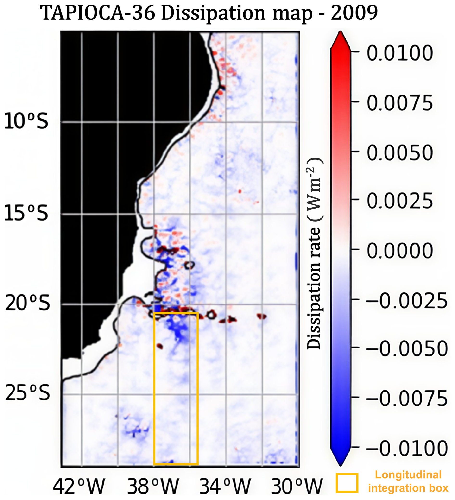
Figure 6 Harmonic dissipation map in 2009 of the VTR region from the TAPIOCA-36 simulation.

This first analysis shows an intense generation of internal tides mostly located in the arc shape of the VTR. With an along track analysis, we deduce that the propagation of internal tides is dominated by the first mode of propagation, at a wavelength of around 131 km, followed by a second mode of propagation with a wavelength of 61 km. The harmonic dissipation mostly refers to the energy contained in the first mode of propagation, which loses most of its energy during its first beam of reflection. Considering that internal tides are fine scale processes, we now aim to further investigate the intra-annual variability of this region and how it may influence internal tides.

3.2 Two contrasted seasons in 2009

The VTR is located at a sub-tropical latitude. Therefore we can expect two contrasted seasons to likely influence the stratification of the water column, mostly due to the Sun radiative forcing variability. In the TAPIOCA-36 simulation outputs, the density profile appears really smooth from May to October, with a density variation of 2 units in 500 m (see Fig. 7). We consider that a permanent pycnocline is located at a depth of around 150 m, where the profile slope breaks slightly. At this depth, we also notice a small bump on the Brunt–Väissälä frequency profile (right panel of Fig. 7). In contrast, from November to April, a seasonal pycnocline appears around 50 m down. During this period, the ocean is strongly stratified: the Brunt–Väissälä frequency reaches a maximum of 0.0006 Hz at 50 m depth. This seasonal stratification has been evidenced recently with in situ observations in Toffoli et al. (2023). Based on these profiles, we define hereafter two contrasted seasons:

1. A season spanning from May to October with a permanent pycnocline at 150 m, also named the winter season hereafter;

2. A season spanning from November to April with the appearance of a seasonal pycnocline at a depth of 50 m, also named the summer season hereafter.

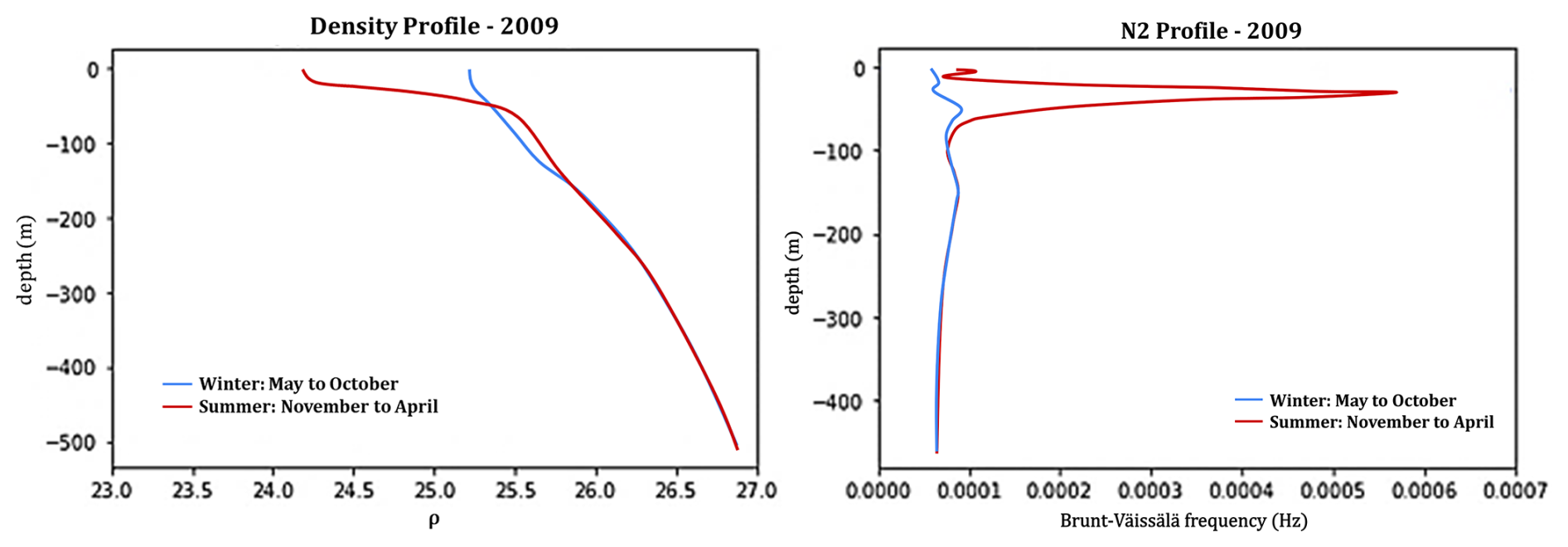
Figure 7 Left panel: Mean density profile around the VTR in the winter season (May–October) and in the summer season (November–April). Right panel: Mean Brunt–Väisälä frequency profile around the VTR in the winter season (May–October) and in the summer season (November–April).

In the following subsections, we will analyze if and how these two contrasted seasons may have an impact on internal tides generated over the bathymetric slope of the VTR.

3.2.1 Generation of internal tides

As the conversion rate C from barotropic to baroclinic energy may also be defined according to the Brunt–Väisälä frequency, the stratification of the water column may influence the generation of internal tides (Baines, 1982; Barbot et al., 2021). In this section, we evaluate the influence of the seasonal changes in the stratification on the generation of internal tides. To achieve this, we integrate spatially the conversion rate in 5 boxes located around the VTR (see Fig. 4) and compute the time averaged conversion rates during the so-called summer season (November–April) and the so-called winter season (May–October) in each box. Apart from the first box located north of the ridge, we observe that the conversion rates are slightly higher in the summer season. More specifically, the differences between the November–April period and the May–October period are the most evident in box 5, i.e. at the ridge extremity, with a variation of 15 % between the two seasons. Even if the relative difference between summer and winter is only about 5 % at the hotspot of generation (boxes 3 and 4), the conversion rates are so high that such a small difference can still impact notably the generation of internal tides (Fig. 8).

Figure 8 Conversion rates integrated within the boxes of the map of Fig. 4 in May–October (in blue) and November–April (in red).

3.3 Propagation

We have seen that the seasonal pycnocline was associated with higher conversion rates from barotropic to baroclinic energy. How does it reflect on the propagation of internal tides? We assess the baroclinic tide propagation by the computation of the baroclinic flux (see Eq. 1), performed by the numerical model. We notice that the baroclinic flux is slightly more energetic during the so-called summer season, consistent with the more intense generation of internal tides from November to April. The baroclinic flux follows the same pattern during both seasons: starting from the VTR, internal tides propagate mainly towards the south until 27° S, that is to say more than 500 km away from the ridge (Fig. 9). Nonetheless, from 23° S the flux is deflected eastward along its course. This deflection could be correlated with the presence of a seamount around 22.2° S or might be influenced by the background circulation, investigated hereafter.

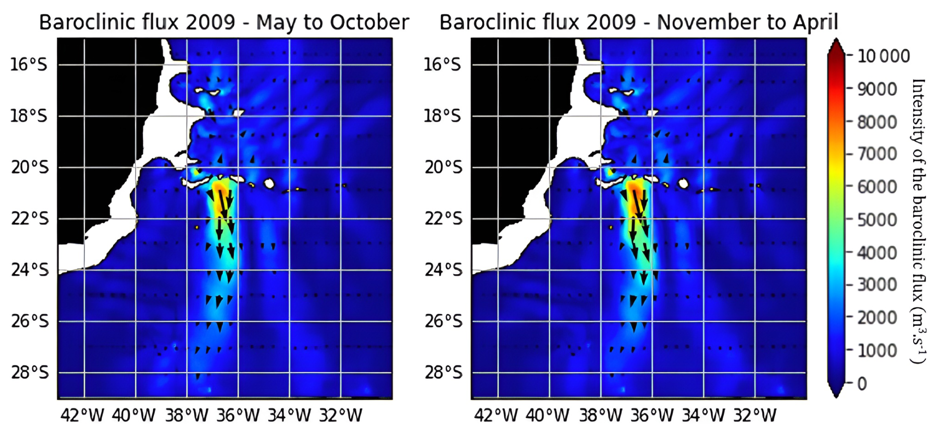
Figure 9 Left panel: Baroclinic flux computed in TAPIOCA-36 for the winter season (May–October). Right panel: Baroclinic flux computed in TAPIOCA-36 for the summer season (November–April).

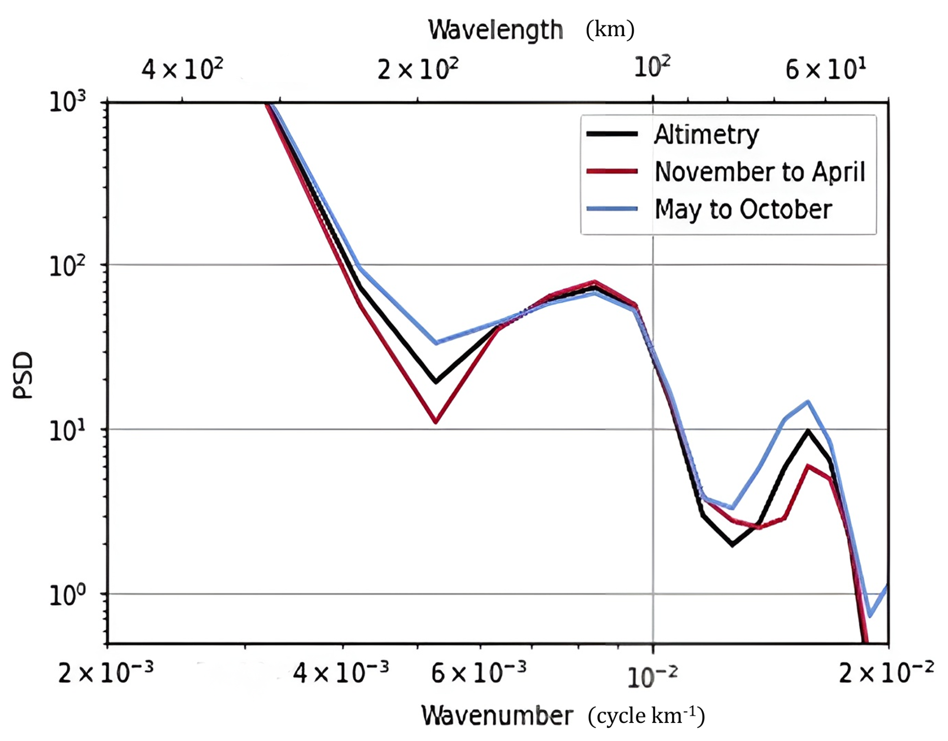
The medium of propagation of internal tides in this region is influenced by a seasonal pycnocline, introducing abrupt changes of the physical properties in the water column near the surface. We investigate if these seasonal changes have an impact on the wavelength of internal tides by using altimetry (see Fig. 10). We conduct a seasonal spectral analysis on the track 137 of the TOPEX/Poseidon mission, presented previously. We take advantage of the 27-year long time series to divide our dataset into two different periods, by gathering the data belonging to the winter (resp. summer) season of each year from 1993 to 2020, reducing the impact of aliasing (Carrère et al., 2004). In Fig. 10, we note that the first mode of propagation keeps the same wavelength over the year, being around 131 km when corrected by the angle at which the altimeter overpasses the internal tides flux. However the second mode of propagation experiences a change: in May–October, the wavelength of the second mode is about 5 km longer than during November–April along the chosen track. On this spectrum, we also notice that the mode-2 of internal tides is more energetic in winter than in summer, with a higher Power Spectral Density. This seasonal variability and its impact on the internal tides' behavior will be discussed in the following section.

Figure 10 Seasonal spectral analysis of the internal tides signal in altimetric data.

3.3.1 Harmonic dissipation

We compute the harmonic dissipation according to the distance from the VTR by integrating longitudinally the dissipation rate inside the yellow box defined on the dissipation map (see Fig. 6). In Fig. 11, we read the integrated dissipation rates according to the latitude. More than 90 % of the baroclinic energy is dissipated after three reflection beams of internal tides. More specifically, during the first reflection, the model does not indicate a strong seasonal variability. The dissipation happening in the summer season might appear slightly higher due to the fact that the generation is more intense during the summer season. However, from 20.9 to 21.7° S, we notice that the dissipation happening in the winter season is 40 % higher than in the summer season. This tendency is inverted after the crossing of the seamount at 22.2° S, where the propagation begins to be more influenced by the second mode of propagation. Further away from the ridge, the dissipation patterns appear more chaotic. An additional peak of dissipation between 22.5–23.5° S is observed during the summer season but is almost absent in winter. We assume that the dissipation happening in the far field from the VTR generation could be influenced by the possible seasonal changes in the background circulation.

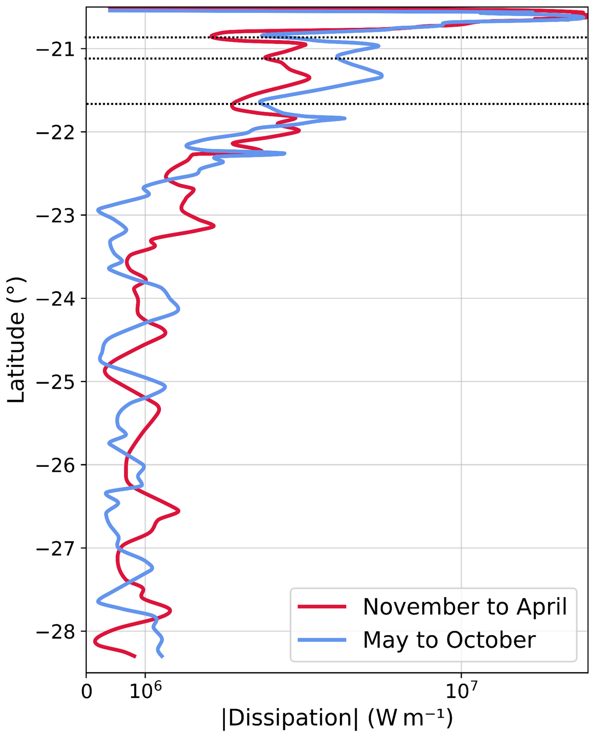
Figure 11 Absolute values of harmonic dissipation rates integrated along the longitude from the TAPIOCA-36 dissipation map in two contrasted seasons displayed on a logarithmic scale. Dotted lines correspond to reflection beams based on the dissipation rates variability.

3.4 Impact of the background mesoscale activity: a qualitative case study

The shape of the baroclinic flux and the spatial chaotic pattern of the internal tides dissipation lead us to investigate the role of the background meso- to submesoscale dynamics, using the TAPIOCA-36 simulation. We plot the daily mean relative vorticity computed at the pycnocline depth and visualize it jointly with the baroclinic flux, in order to evaluate whether the internal tides could interact with other ocean processes in this turbulent region.

By looking at snapshots over the year 2009, we spot a mesoscale anticyclonic eddy entering the propagation area of the main baroclinic flux on the 13 February 2009. The center of this eddy is arriving from the open sea and evolving westward to the Brazilian coast along the 23.5° S parallel, where we highlighted a peak of dissipation between November–April (see Fig. 11). We follow the course of this anticyclonic eddy by selecting four key moments, corresponding to similar tidal regimes. On the 27 February, the baroclinic flux starts to be deflected by about 25° towards the east when crossing the eddy at its center, as if the energy was trapped and concentrated by the anticyclonic eddy. On the 13 March 2009, the eddy is located directly south of the internal tide generation hotspot. The associated baroclinic flux mainly propagates southwards but is also slightly deflected towards the east and the west. On the 12 April 2009, the eddy finally escapes the main internal tides propagation area and deflects the flux by about 25° towards the west.

4 Discussion

In this study, we employed a dynamical model to evaluate the seasonal variability in the generation of internal tides at the VTR. By analysing the monthly stratification profiles provided by our model, we show that a sharper stratification during November–April is linked to an increase in the generation of internal tides, compared with the May–October period. This result aligns well with the the study of Qian et al. (2010). Toffoli et al. (2023) recently gathered in situ observations on the main generation site of the VTR over each month of the year, corresponding to the box 3 in Fig. 4. Their observation dataset suggests that conversion rates are strongly linked to the stratification variability. Other internal tides generation sites in the global ocean have shown that the background stratification impacted the generation of internal tides (Barbot et al., 2021). Based on the stratification profiles at the internal tides generation hotspot, we defined two seasons, dividing a full year into two 6-month time periods. Although Toffoli et al. (2023) analysed the impact of the stratification on only 2-month periods, we note a discrepancy in the intra-annual variability at the VTR between their observations and our results. Even if in situ measurements are invaluable at this location, the fact that they were acquired over 12 months but across two separate years (2016 and 2018) may introduce some uncertainties, while our model simulation was performed on a complete year being 2009, almost 10 years apart from their last measurements. A better understanding of the oceanic inter-annual variability at this specific location would be useful to provide insights on the modulation of internal tides generated at the VTR.

Additionally, we have shown that the internal tides at the VTR were mostly dominated by the first mode of propagation, which does not seem to be influenced by stratification changes. According to Barbot et al. (2021), the mode 2 of propagation is likely more sensitive to seasonal changes, with a tendency to be longer during the less stratified season. Here, we also observed in altimetric data that the energy linked to the second mode of propagation decreases slightly during the November–April period (summer). In the previous section, we also saw that the dissipation of internal tides was greater locally during this same period. While these slight differences may be linked to the geographical orientation of the selected track, another factor could also be that a strong stratification confines the mode 2 to a shallow vertical region, making it more sensitive to dissipation and preventing this mode to propagate further away from the ridge. Hence, as the baroclinic flux is still appearing more intense from November to April in our simulation, we suppose that the internal tides signal may be dominated by the first mode of propagation, as it is also supported by the study of Toffoli et al. (2023).

At 22.2° S, the presence of a seamount on the internal tides propagation path might also play a role in the energy dissipation pathways and in the transfer of energy from the mode 1 of propagation to the mode 2 of propagation. Indeed, a shift in the wavelengths of the reflection beams is both observed in altimetry and modeled in our regional simulation displayed in Fig. 5. This topographical abrupt feature may drive an energy cascade from the first to the second mode of propagation by scattering the baroclinic energy. This phenomenon has already been identified at the North Mid-Atlantic Ridge in the study of Lahaye et al. (2020). As a result, additionally to the stratification variability, topography may also modulate the fate of internal tides generated at the VTR.

Finally, our study highlights that the mesoscale activity of the region may also influence the internal tides flux propagating in the region. More specifically, we describe the case of an eddy propagating through the internal tides flux from February to April 2009. This first qualitative result supports the assumption that internal tides of this turbulent region may also be influenced by external forcings, through interactions with mesoscale processes. Several other studies highlighted internal tides-eddy interactions, including one depicting how a mesoscale eddy can induce straining on internal waves in the Southern Ocean, resulting in the energizing of the eddy itself (Cusack et al., 2020). In contrast, another regional study showed the depletion of an eddy by internal waves in the North Atlantic Ocean, where internal waves appeared to dissipate its kinetic energy (Barkan et al., 2021). More recently, Kouogang et al. (2026) and Goret et al. (2026) have shown that internal tides modeled off the Amazon shelf could be deviated, and even scattered by the presence of an intense mesoscale eddy. To better understand the behavior of internal tides at these subtropical latitudes, a more quantitative work involving both modeling and observations would be necessary. In particular, the Cal/Val period of the SWOT mission could be an opportunity to investigate such internal tides-eddy interactions with an increased resolution. This type of interaction is of interest because it drives cross-scale energy transfers, which must be quantified to close the ocean energy budget (Delpech et al., 2024).

5 Conclusion

In this study, we describe and analyse internal tides generated at the VTR thanks to the combination of two validated tools: a high resolution regional oceanic model (TAPIOCA-36) and a long time series of satellite altimetry data. These two valuable approaches are complementary and show an undeniable agreement on the SSH elevation linked to the M2 component of the internal tides. Indeed, they both display the same six reflection beams linked to the first (north of 22.2° S) and second mode (south of 22.2° S) of propagation south of the VTR. Altimetry provides estimates of the wavelength of each mode of propagation: 131 and 61 km for the first and second modes of propagation respectively. The TAPIOCA-36 simulation helped to understand the properties of internal tides in the region at a high spatio-temporal resolution, from their generation to their dissipation.

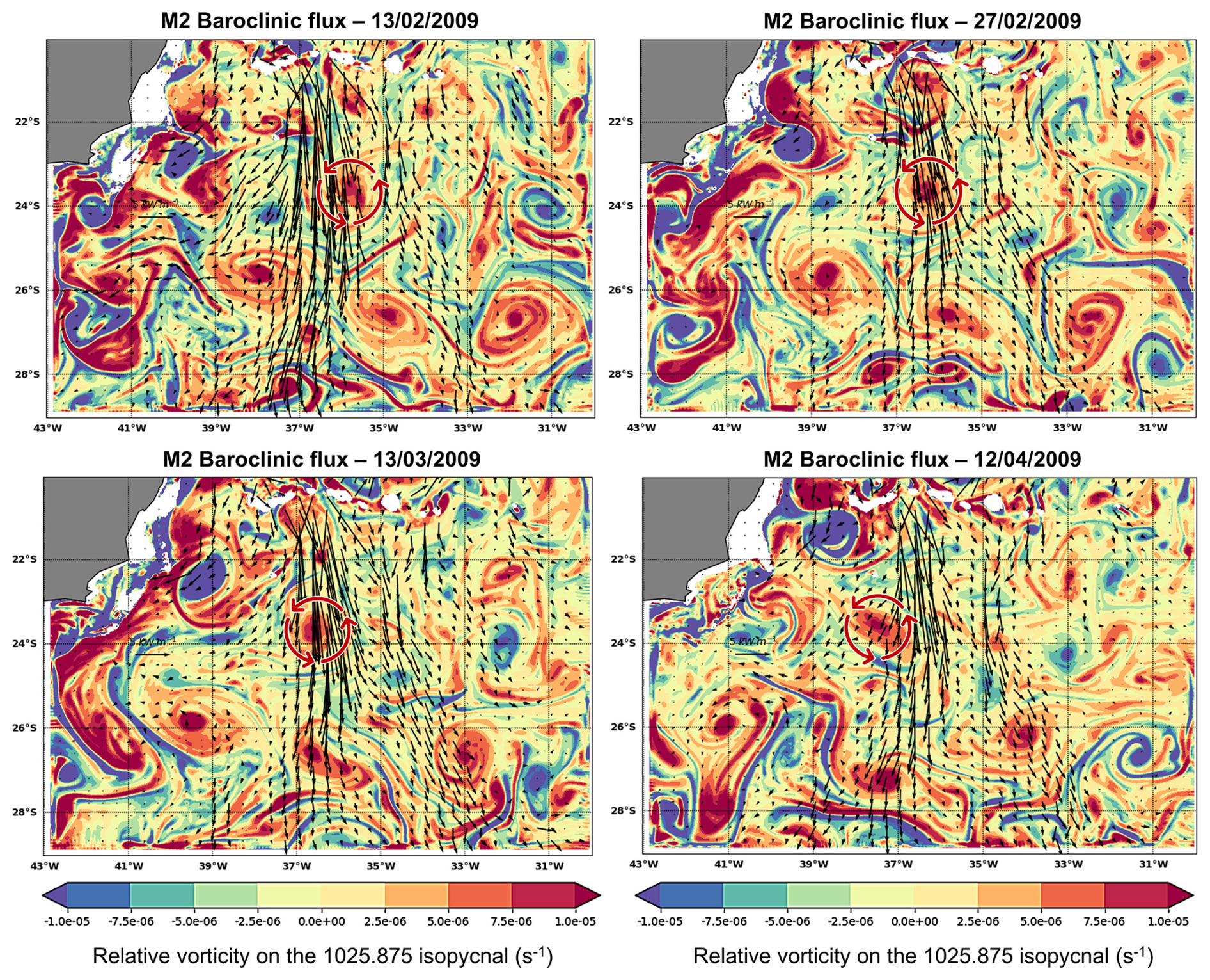
Figure 12 Time evolution of a mesoscale eddy crossing the baroclinic flux (black arrows). The background is the relative vorticity projected onto the pycnocline. Upper left panel – 13 February 2009: the eddy is entering the propagation area. Upper right panel – 27 February 2009: the baroclinic flux is crossing the eddy. Lower left panel – 13 March 2009: the baroclinic flux is deviated from one side to another by the eddy. Lower right panel – 12 April 2009: the eddy is leaving the propagation area.

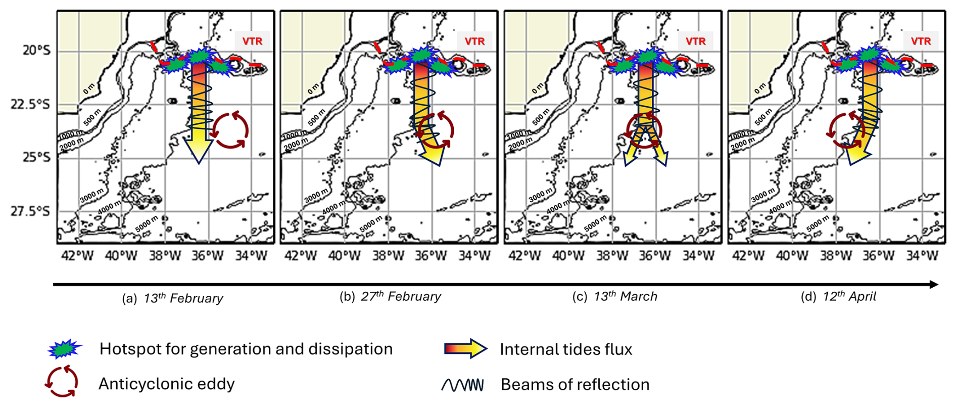
Figure 13 Schematic representation of a case of interaction between internal tides and a mesoscale eddy between the 13 February 2009 and the 12 April 2009, south of the VTR.

Over the year 2009, we identified two contrasted seasons: a summer season associated with a shallower seasonal pycnocline and an increase in the Brunt–Väisälä frequency from November to April; and a winter season characterized by a smoother stratification from May to October. Using our ocean model simulation over 2009, we find that more barotropic energy is converted into baroclinic energy during the summer season of this year, resulting in a more intense baroclinic flux. A qualitative case-study displays how the background circulation and mesoscale activity can modulate the internal tides flux south of the VTR. Seasonal stratification changes also impact the propagation of internal tides. In particular, altimetric data record a slight change in the wavelength of the second mode of propagation, being 5 km longer during winter than summer.

Finally, we describe the dissipation pattern of the baroclinic energy, which occurs mostly close to the generation site with 45 % of the baroclinic energy dissipated locally. However, away from the ridge, our study show that dissipation rates are higher during the winter season than during the summer season. We notice that the propagation path of internal tides is actually subjected to intermittent strong eddies and jets. In particular, we study the evolution of a mesoscale eddy crossing the propagation path of internal tides and propagating towards the Brazilian coast, summarized in Fig. 13. During this sequence, the baroclinic flux is deflected by the anticyclonic eddy, first towards the east (b) and then towards the west when the eddy is moving away from the propagation area of internal tides (d). This eddy resolved by our ocean model influenced the propagation of the internal tides. Reciprocally, internal tides seemed to hinder the evolution of the eddy towards the coast by interacting with it. These preliminary qualitative results are in line with the results of Dunphy and Lamb (2014), and more recently of Tchilibou et al. (2022). Figure 13 provides a schematic representation of this interaction, highlighting the mutual influence between the eddy and internal tides and offering a visual summary of the described dynamics.

This paper provides an overview of the meso- to submesoscale dynamics in this turbulent region, which had never been studied before with the combination of a regional dynamical high-resolution model and long altimetric time-series. Internal waves and mesoscale eddies are known to represent large reservoirs of kinetic energy: they play an important role for energy redistribution and hence climate regulation (Ferrari and Wunsch, 2009). The increase in computational resources and the innovation in our observation systems has nowadays improved knowledge on smaller oceanic processes and their energetic transfers (Bauchot, 2025; Martin et al., 2023), but the ocean energy budget is still to be closed and physical oceanic interactions at meso- to submesoscales are still to be unveiled. In the context of the SWOT mission, new direct observations will probably enable to characterize the energy transfers linked to internal tides over the region at a time and space resolution never reached before (Tchilibou et al., 2025). However, the study of internal waves also requires in situ measurements within the water column, and this was the aim of the recent work of Toffoli et al. (2023) and the recent Abrolhos campaign (Hernandez et al., 2025). In line with this work, a synergistic approach combining high-resolution modeling, remote sensing including SWOT data, and in situ observations will remain essential to fully understand the dynamics and energy pathways in this complex and understudied region.