Gliding through marine heatwaves: subsurface biogeochemical characteristics on the Australian continental shelf

Marine heatwaves (MHWs) disrupt ecosystems across multiple trophic levels by altering oxygen and biological productivity through the water column and yet, most studies focus on the surface, overlooking subsurface processes that shape ecosystem responses. To address this gap, we analysed 16 years of routine and event-based glider observations on the continental shelf around Australia to present the first comprehensive assessment of the subsurface biogeochemical response during surface MHWs across four contrasting coastal regions. Across all regions and seasons, the distribution of chlorophyll concentrations shifted towards a decline in the mixed layer and an increase below the mixed layer during MHWs, modulated by the event categories. Dissolved oxygen shows a more complex distribution, which also varies during moderate and strong MHW events, arguably with more variation in the mixed layer than below. When regional and seasonal specificities are taken into account, the subsurface characteristics of MHWs vary in accordance with the environmental setting, including the continental shelf structure, tropical or sub-tropical regime, and boundary current influence, especially through the changes in stratification. Summer surface MHWs were characterised by a shallower mixed layer depth than normal conditions and enhanced stratification, confining warming to the upper ocean, while other seasons allow deeper penetration under weakly stratified conditions. The depth of maximum stratification therefore emerged as a useful proxy for the vertical extent of MHWs. The interaction between physical processes, such as seasonal circulation and stratification, and biological feedback, including the presence of deep chlorophyll maxima and potential oxygen production, highlights the complex biogeochemical responses to MHWs, and underscores the importance of region-specific dynamics and the need for more consistent observation strategy, including biogeochemical processes.

1 Introduction

As the Earth's climate continues to warm, the frequency and intensity of extreme events are increasing due to anthropogenic forcing (Frölicher et al., 2018; Laufkötter et al., 2020) with profound consequences for both ecosystems and human societies (Smith et al., 2021, 2023). Marine heatwaves (MHWs) are defined as extremely warm ocean temperature anomalies and have become an increasing focus of research for their important impacts on ecosystems (Capotondi et al., 2024). A key factor controlling MHW characteristics, including their vertical extent, intensity and persistence, is upper-ocean stratification (Schaeffer and Roughan, 2017; Schaeffer et al., 2023; Zhang et al., 2023). Global stratification has intensified over recent decades, leading to widespread mixed layer shoaling and altered thermocline structure (Capotondi et al., 2012; Li et al., 2020; Kwiatkowski et al., 2020; Amaya et al., 2021; Zhang et al., 2023). At regional and coastal scales, stratification is further shaped by local thermal, salinity and mechanical processes that regulate the vertical mixing and influence the occurrence of MHWs (Fordyce et al., 2019; Amaya et al., 2021; Gao et al., 2020; Schaeffer et al., 2023). Recent studies have shown that subsurface signatures of MHWs can differ substantially from surface observations. For instance, during the 2019 North Pacific MHW (“The Blob”), subsurface warming persisted long after surface temperatures returned to normal, leading to prolonged ecological stress at depth (Amaya et al., 2020). Similarly, along the east coast of Australia in New South Wales, subsurface MHWs have been documented with minimal surface expression, highlighting the need for vertical profiling, particularly in coastal regions where strong stratification, complex circulation and shallow bathymetry can amplify subsurface temperature anomalies (Schaeffer et al., 2016a, 2023). Strong stratification can trap heat near the surface or isolate warm anomalies below the mixed layer, allowing subsurface MHWs to persist at depth.

Investigating subsurface dynamics of MHWs in coastal areas is therefore critical for assessing ecological and socio-economic impacts. In coastal regions and over continental shelves, subsurface biogeochemical processes play a central role in sustaining vital ecosystem services such as biodiversity, carbon sequestration and nutrient cycling, while supporting economic activities such as fisheries and aquaculture (Walsh, 1991; Siefert and Plattner, 2004; Marre et al., 2015). When combined with MHWs, biogeochemical extremes can trigger severe ecological disruption, amplifying existing environmental stressors, such as nutrient limitation (Cavole et al., 2016; Le Grix et al., 2021), acidification, and deoxygenation (Tassone et al., 2022), ultimately reducing productivity and threatening marine ecosystem health.

Understanding how MHWs influence key biogeochemical variables, such as chlorophyll a concentrations (proxy for phytoplankton concentration; Blondeau-Patissier et al., 2014) and oxygen levels, is essential for predicting ecosystem responses. For instance, nutrient scarcity during MHWs can limit phytoplankton growth, while warmer waters increase metabolic demands in marine species, further straining ecosystems (Chen et al., 2023). Although surface chlorophyll a often decreases during MHWs (Le Grix et al., 2021), responses vary depending on factors such as light and nutrient availability (Sen Gupta et al., 2020; Noh et al., 2022). In regions where stratification limits nutrient upwelling, phytoplankton productivity may decrease, whereas, at higher latitudes (where light is a limiting factor), stratification can enhance productivity by maintaining phytoplankton in the sunlit surface layers (Kwiatkowski et al., 2020). On a global scale, MHWs have been found to promote the development of deep chlorophyll maxima, based on 17 years of biogeochemical-Argo float data (Ma and Chen, 2025). Reduced dissolved oxygen during MHWs represents another critical issue, particularly in shallow coastal areas. Warmer water temperatures decrease oxygen solubility, potentially leading to hypoxic conditions that can severely affect marine life (Meier et al., 2018; Safonova et al., 2024). MHWs intensify this mismatch between oxygen supply and demand, as respiration rates increase in response to higher temperatures, further depleting oxygen levels (Tassone et al., 2022). Combined effect of MHWs, reduced oxygen levels, and habitat compression can trigger mass mortality events across multiple taxa, including fish, seagrasses, and marine mammals (Sampaio et al., 2021; Holbrook et al., 2022), while altered prey distribution and increased metabolic demands can produce cascading effects throughout marine food webs (Smith et al., 2023; Gomes et al., 2024).

While long-term satellite-derived records of sea surface temperature (SST) and surface chlorophyll a have advanced our understanding of MHWs globally, they require concurrent in water measurements to assess the extent of subsurface temperature extremes and biogeochemical changes given the range of ecological impacts that can occur through the water column (Smith et al., 2023). Traditional in situ methods such as moored temperature measurements, conductivity-temperature-depth, and expendable bathythermograph casts can provide vertical profiles, but these observations are often limited in spatial and temporal coverage (Oliver et al., 2021; Malan et al., 2025; Le Gendre et al., 2025) and rarely include biogeochemical observations. In addition, coastal numerical models offer valuable simulations of subsurface thermal structures, but they require large amounts of high-resolution data for validation or assimilation, as they remain prone to uncertainties in poorly observed regions (Lachkar et al., 2019).

Ocean gliders offer a major advancement in subsurface monitoring, through high-resolution, autonomous, and continuous measurements of water temperature, salinity, and biogeochemical properties, including dissolved oxygen and chlorophyll fluorescence (Testor et al., 2019). Although glider deployments have limited temporal coverage for detecting extremes, their ability to sample across depths and regions provides an unprecedented view in shelf and boundary current environments (Testor et al., 2019). These measurements can be used to infer stratification and phytoplankton dynamics. Furthermore, event-based approaches, where gliders are deployed specifically to sample MHWs, can provide real-time, dynamic insights into the subsurface evolution and intensity of these events, delivering essential input to immediate ecosystem response strategies (Davies, 2021; Benthuysen et al., 2025). Previous studies have made notable strides on better understanding the subsurface dynamics and biogeochemical variability using gliders off the Australian coast (Pattiaratchi et al., 2011; Schaeffer et al., 2016a, b; Chen et al., 2019; Chen et al., 2020; Ridgway and Ling, 2023). However, most of these works focused on specific regions off the Australian coast or were limited to specific events, typically ranging from weeks to months, rather than continual monitoring. While these studies did not explicitly focus on MHWs, gliders have been demonstrated as a useful platform to capture the vertical extent of extreme warming, such as during the 2016 austral summer MHW off northeastern Australia (Benthuysen et al., 2018), highlighting the role of glider observations to inform MHW studies.

To address this gap, our study leverages data from the Australian Integrated Marine Observing System (IMOS) gliders which provide high-resolution subsurface observations along the Australian continental shelf since 2007 (Pattiaratchi et al., 2017). By combining these repeated glider measurements with satellite-derived surface data, we aim to provide a seasonal and regional comparison across four distinct Australian shelf regions, highlighting broader patterns of subsurface MHW characteristics and their impacts on key biogeochemical variables. Specifically, we test the following hypotheses: (1) surface MHWs can lead to reduced chlorophyll concentrations and lower dissolved oxygen levels at the surface; (2) despite surface reductions, MHWs may promote deeper chlorophyll maxima and higher dissolved oxygen concentrations at depth, potentially via enhanced subsurface productivity; (3) the depth extent of surface MHWs varies with regions and seasons, and therefore establishing seasonal and regional baselines are important to interpret anomalies; and (4) the severity of MHW-induced stratification modulates biogeochemical variables (dissolved oxygen and chlorophyll).

The following sections outline our approach and findings: Sect. 2 describes the SST and glider datasets, statistical methods, and MHWs metrics. Section 3.1 describes the characteristics of surface MHWs in the study regions. Hypotheses (1) and (2) are examined in Sect. 3.2, which investigates how MHW severity influences chlorophyll and dissolved oxygen within and below the surface mixed layer. Hypothesis (3) is addressed in Sect. 3.3, where we explore regional and seasonal variations in the depth extent of MHWs, stratification and associated biogeochemical profiles. Hypothesis (4) is evaluated across Sect. 3.2 and 3.3, which together assess how MHWs modulates subsurface biogeochemical signatures in different regimes, based on their stratification, chlorophyll and oxygen regimes. Finally, Sect. 4 discusses these findings in the context of previous global and Australian studies, leading to the Conclusions in Sect. 5.

2 Data and Methods

2.1 Satellite dataset and surface MHW detection

Given the coastal scale of our study, we used the National Oceanic and Atmospheric Administration (NOAA) CoralTemp v3.1 (CoralTemp v3.1 product's website: https://coralreefwatch.noaa.gov/product/5km/index.php, last access: 28 February 2026) Sea Surface Temperature (SST) product, which integrates three L4 satellite SST analysis products, to provide a global, daily, gap-free gridded, night-time SST field at 0.05° horizontal resolution since 1985 (Skirving et al., 2020). This dataset is used to track surface MHWs in near real-time (NOAA Coral Reef Watch marine heatwave website: https://coralreefwatch.noaa.gov/product/marine_heatwave/, last access: 28 February 2026) using the definition and criteria of Hobday et al. (2016), which detects temperature events exceeding a locally determined upper threshold of the 90th percentile relative to the long-term day-of-the-year climatology for a minimum of five consecutive days, with no gap of more than two days. The baseline climatological period was defined here as a 30-year period between 1985 and 2014, following recommendations of Hobday et al. (2016). The MHW detection and analysis were performed using the Python module available at https://github.com/ecjoliver/marineHeatWaves (last access: 28 February 2026). We extracted the SST dataset over the period from 1 January 1985 to 30 June 2025 and the following MHW metrics were analysed over our study period from 2009 to mid-2025: the total number of events, the mean duration of the MHW events, and the mean severity of the MHW (Eq. 1; following Sen Gupta et al., 2020).

2.2 Glider dataset

To assess the subsurface structure of MHWs, our study benefited from the Australian national glider data acquisition strategy set up in 2007 by the Ocean Gliders facility under IMOS (Pattiaratchi et al., 2017). Subsequently, IMOS enabled the routine deployment of gliders on the continental shelves around Australia for sustainable observations. This facility has been augmented by event-based sampling of MHWs since December 2018 (Benthuysen et al., 2025), delivering subsurface measurements of oceanographic parameters along with other near-real time platforms during events (e.g. Box 2 of Capotondi et al., 2024). Ocean gliders are autonomous vehicles which alter their buoyancy to travel up and down the water column while sampling seawater properties (Rudnick, 2016). We used data from IMOS using Teledyne Webb Research Slocum Electric Gliders (G1, G2 and G3), equipped with Seabird-CTD, WETLabs BBFL2SLO 3 Eco Puck sensor measuring chlorophyll fluorescence, colored dissolved organic matter (CDOM) and 660 nm backscatter, and an Aanderaa Oxygen optode (Pattiaratchi et al., 2011; Chen et al., 2020). Missions typically last between three to five weeks, with a maximum depth of 200 m. For this study, we focus on measurements of ocean temperature, salinity, chlorophyll a fluorescence, and dissolved oxygen. The measurements undertake a delayed-mode quality control (Woo and Gourcuff, 2021) and are made publicly available through IMOS on the Australian Ocean Data Network (AODN) Portal (Australian Ocean Data Network (AODN) website: https://portal.aodn.org.au/, last access: 16 September 2025).

2.3 Study regions

The analysis of all available deployments led us to the definition of four main regions of interest encompassing the highest density of gliders transects between 2009 and 2025: (i) northeastern Australia off Queensland (QLD), confined within the limits of 144.7 to 148.0° E and 13.3 to 19.7° S; (ii) southeastern Australia off New South Wales (NSW), from 149.7 to 154.7° E and 28.5 to 36.7° S; (iii) southwest Western Australia (SW WA), from 113.2 to 116.1° E and 29.1 to 33.5° S; and (iv) the eastern coast of Tasmania (TAS), from 146.8 to 149.5° E and 40.5 to 44.6° S (Fig. 1). These regions encompass contrasting continental shelf systems influenced by distinct physical processes, enabling us to assess how MHWs impact biogeochemical conditions under different dynamics.

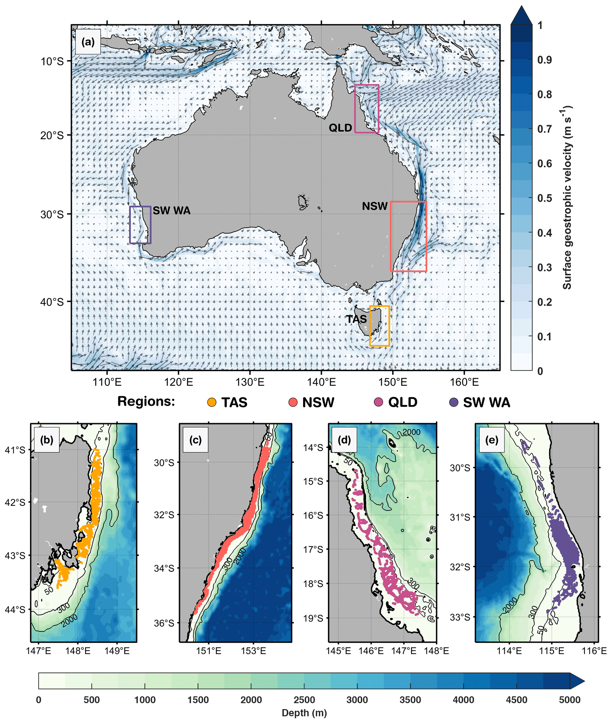
Figure 1 Study regions off the Australian coast. (a) Mean surface geostrophic currents (arrows) and highlighted boxes for each region of interest: eastern Tasmania (TAS), southeastern Australia (New South Wales, NSW), northeastern Australia (Queensland region, QLD), and southwest Western Australia (SW WA). Gliders' profile positions are illustrated in each sub-region: (b) TAS, (c) NSW, (d) QLD and (e) SW WA. In (a), the annual mean geostrophic currents were based on 1993 to 2020 and provided by the Integrated Marine Observing System (IMOS, https://imos.aodn.org.au/oceancurrent, last access: 4 December 2025). Isobaths of 50, 300, and 2000 m are shown in (b)–(e), derived from ETOPO1 bathymetry (Eakins and Sharman, 2010). Glider profiles are located over the continental shelf, in waters shallower than 200 m isobath.

2.4 Profile selection and data processing

Glider deployments were selected to keep only those profiles within the aforementioned study regions, spanning a 16-year period from January 2009 to June 2025. To ensure the quality of our analyses, the following quality control steps were taken for each glider mission: (i) selection of only “good data” flags (Woo and Gourcuff, 2021) (https://content.aodn.org.au/Documents/IMOS/Facilities/Ocean_glider/Delayed_Mode_QAQC_Best_Practice_Manual_OceanGliders_LATEST.pdf, last access: 16 September 2025); (ii) removal of chlorophyll outliers; (iii) applying a step to address non-photochemical quenching in chlorophyll observations; and (iv) removal of data points inside the bottom boundary layer (BBL). To remove the noise from the chlorophyll measurements (step ii), the outliers were identified based on a moving average of window size equivalent to 1000 points along the glider sampling, discarding values above two standard deviations of the logarithmic chlorophyll. Moreover, light-induced fluorescence leads to errors in sensor measurements of phytoplankton concentration (quenching), causing high variability in chlorophyll a fluorescence profiles. To mediate this effect (step iii), we used only night-time data points, defined as any time before sunrise or after sunset (as in Schaeffer et al., 2016a). Regarding the variable BBL contamination due to sloping topography, we removed data within 20 m above the seabed, similar to Schaeffer et al. (2014, 2016a). This threshold aims to minimize contamination from interference in the near-bottom levels when aggregating the shelf profiles over various topographic depths for a combined analysis.

This study is focused on continental shelf waters, and hence the few measurements from deeper regions were excluded. The continental shelf width and depth at the shelf-edge varies over each region. Off QLD and SW WA, only measurements over bathymetry between 40 and 80 m were retained. For regions with deeper and steeper continental shelves, i.e. TAS and NSW, we retained measurements between 50 and 120 m. Finally, we separated the data points into downward and upward casts, binned each cast into a 1 m vertical resolution, averaged each pair of down/upward casts, and binned the averaged profiles into fixed distances of 1 km horizontal resolution, which is more than the median distance between profiles (e.g. 100–200 m in NSW region, Schaeffer et al., 2016a). These last steps enable vertical and horizontal consistency of profiles, avoid glider's direction bias when averaging the down/upward casts, and reduce noise for shelf-scale comparison of subsurface MHW signals. In Fig. S1 in the Supplement, we illustrate a glider mission before and after quality control steps mentioned above.

2.5 Classifying MHW vs non-MHW profiles

We classify MHW and non-MHW glider profiles by first collocating surface MHW severity index in time and space using the satellite SST dataset. Thus, the severity index (S) was calculated for each profile following Sen Gupta et al. (2020), as below:

$$\begin{array}{}\text{(1)}& S_{i,d}={\displaystyle \frac{{\mathrm{SST}}_{i,d}-{\mathrm{SST}}_{i,d}^{\mathrm{clim}}}{{\mathrm{SST}}_{i,d}^{\mathrm{PC}\mathrm{90}}-{\mathrm{SST}}_{i,d}^{\mathrm{clim}}}}\end{array}$$

where SST${}_{i,d}^{\mathrm{clim}}$ is the long-term daily mean SST on the dth day of the year at location i, ${\mathrm{SST}}_{i,d}^{\mathrm{PC}\mathrm{90}}$ is the 90th percentile of SST on the same day and location as the glider profile. The MHWs were categorised into four types: (i) moderate, 1 < S ≦ 2; (ii) strong, 2 < S ≦ 3; (iii) severe, 3 < S ≦ 4, and (iv) extreme (S > 4) following the category indices proposed in Hobday et al. (2018). For each study region, the mean location of the glider profiles was determined, and time series of the severity index were derived, enabling the representation of an “average” severity timeline for each region (see Fig. 1b–e).

2.6 In situ subsurface parameters

To further characterise the surface-MHWs in subsurface layers, some proxies were used, such as: (i) mixed layer depth (MLD); (ii) thermocline depth; (iii) buoyancy frequency, i.e. degree of stratification; (iv) dissolved oxygen saturation; (v) MHW depth extent, defined as depth containing 90 % of the vertical heat content anomaly; (vi) depth of maximum stratification, defined as the depth at which the buoyancy frequency reaches its maximum value in the water column; and (vii) depth of deep chlorophyll maxima (DCM). For anomaly calculations in the subsurface, we used non-MHW profiles as our baseline, i.e. anomalies were calculated relative to the mean non-MHW profile. This provided a physically consistent background state and avoided potential bias introduced by uneven sampling of MHW and non-MHW profiles. Therefore, we defined the seasonal mean composite for each region as the average non-MHW profiles over three-month seasonal periods (austral summer – December/January/February, autumn – March/April/May, winter – June/July/August, and spring – September/October/November).

The MLD was computed for each individual temperature profile by identifying the shallowest depth at which the absolute temperature difference from the surface (0 m) exceeded a fixed threshold of 0.2 °C. This threshold-based method is commonly applied to in situ observations due to its physical relevance in stratified ocean conditions (e.g., de Boyer Montégut et al., 2004). Profiles with missing surface data or insufficient vertical resolution near the surface were excluded from MLD calculations. MLD estimates were then averaged seasonally and grouped into MHW and non-MHW categories, based on the presence or absence of surface MHW conditions.

The thermocline depth was computed from the vertical temperature profiles by calculating the temperature gradient with respect to depth. The depth corresponding to the maximum negative gradient (i.e. the strongest rate of temperature decrease with depth) was defined as the thermocline depth.

The buoyancy frequency, also called the Brunt Väisälä frequency, represents the degree of stratification and is defined as:

$$\begin{array}{}\text{(2)}& N^{\mathrm{2}}=-{\displaystyle \frac{g}{{\mathit{\rho }}_{\mathrm{0}}}}{\displaystyle \frac{\partial \mathit{\rho }}{\partial z}}\end{array}$$

where ρ₀ represents the background density, g is the gravitational constant and $\frac{\partial \mathit{\rho }}{\partial z}$ denotes the vertical gradient of potential density. The density was calculated from the glider's vertical temperature and salinity profiles.

Dissolved oxygen saturation was computed from temperature, salinity and pressure following standard solubility formulations, using the García and Gordon (1992) equation for seawater. Hence, oxygen saturation was calculated as the ratio between measured dissolved oxygen concentration and the corresponding solubility value at in situ conditions. This provides a temperature- and salinity-adjusted measure of oxygen availability relative to atmospheric equilibrium, making it a useful indicator of both biogeochemical processes (production and respiration) and physical transport mechanisms (vertical mixing and horizontal advection) that influence oxygen independently of solubility changes.

MHW depth extent was defined as the depth which contained 90 % of the vertical heat content anomaly, following Elzahaby and Schaeffer (2019). For each MHW profile, positive temperature anomalies (ΔT>0) were integrated vertically, and the depth extent corresponded to 90 % of the profile's cumulative temperature anomaly. This approach provides a physically consistent estimate of the vertical penetration of the MHW-associated warming relative to background (non-MHW) conditions.

To evaluate the relationships between physical and biogeochemical variables during MHWs, we calculated the correlations over profiles by regions and seasons separately. The variables considered include MHW depth extent, depth of maximum stratification, depth of DCM, thermocline depth, dissolved oxygen (DO) anomalies, chlorophyll (CHL) anomalies, and temperature anomalies above and below the MLD. Several restrictions were applied to ensure that the correlations were unbiased.

• i.

  Only stratified profiles were retained, when the profile maximum buoyancy frequency (N²) exceeded the 75th percentile of the regional distribution of maximum N² values. This approach excludes homogeneous and weakly stratified profiles, often present in winter, that would otherwise give false strong correlations.

• ii.

  Profiles lacking any positive subsurface temperature anomalies, since some of these metrics are undefined in these cases and their inclusion would bias correlations toward spurious zero-inflation.

• iii.

  Depths shallower than 5 m and within 5 m from the bottom were excluded to avoid surface and near-bottom artefacts.

• iv.

  Correlations were considered significant only if the p-value was less than 0.05 and the number of data points (profiles) was greater than 30 (Fig. S8).

2.7 Summary of glider missions

Across the four study regions, a total of 202 glider missions were recorded over the continental shelf between January 2009 and June 2025, with the highest number off SW WA (77 glider missions) and NSW (56 missions), followed by TAS (41 missions) and QLD (27 missions). These missions yielded 61 280 profiles (Table 1), with NSW and SW WA contributing the largest to the dataset (19 785 and 19 355 profiles, respectively), and fewer profiles in TAS (11 699) and QLD (10 441). These glider missions and their associated profiles were distributed seasonally, with and without MHW encounters (Table 1, Fig. 2b, d, f, h). Note that the number of chlorophyll profiles is lower than for other variables because of (i) quality control steps, (ii) removal of chlorophyll outliers and (iii) fluorescence quenching as described in Sect. 2.4, and these data are presented in Table S1.

Table 1 Seasonal number of profiles with and without MHWs by region, as eastern Tasmania (TAS), southeastern Australia (New South Wales, NSW), northeastern Australia (Queensland region, QLD), and southwest Western Australia (SW WA).

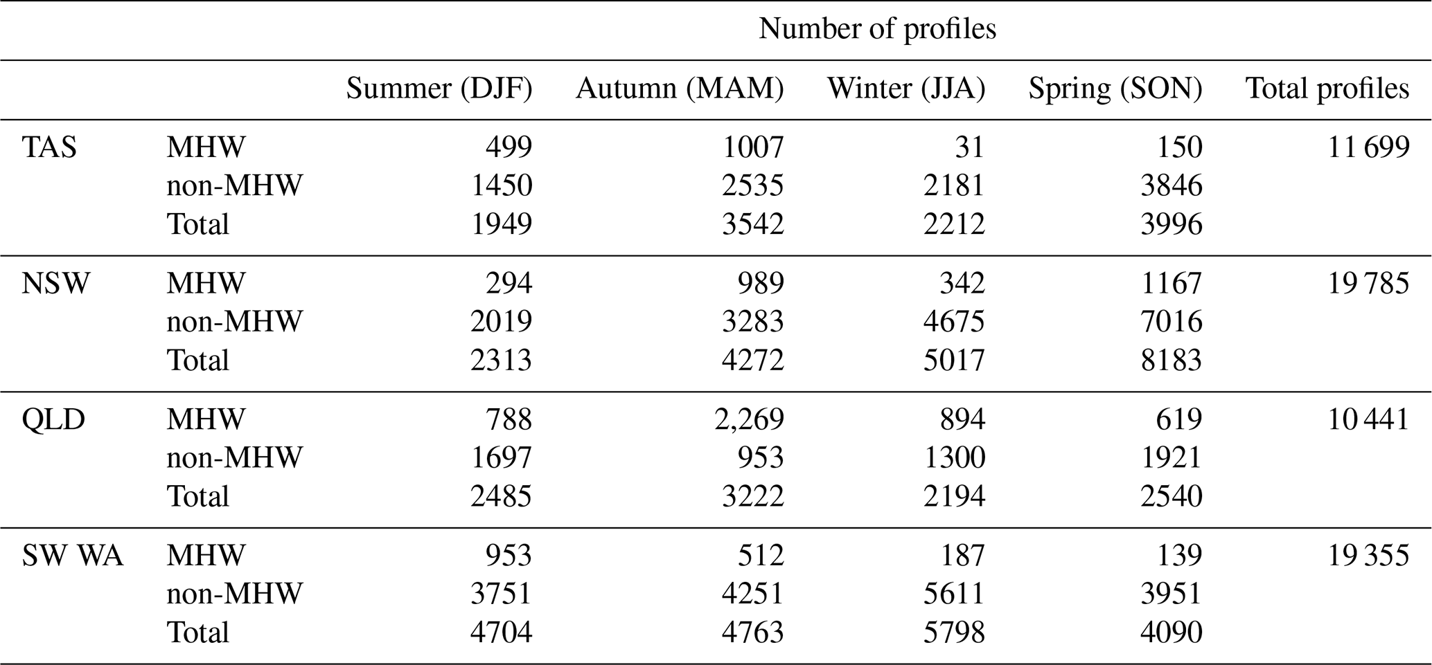
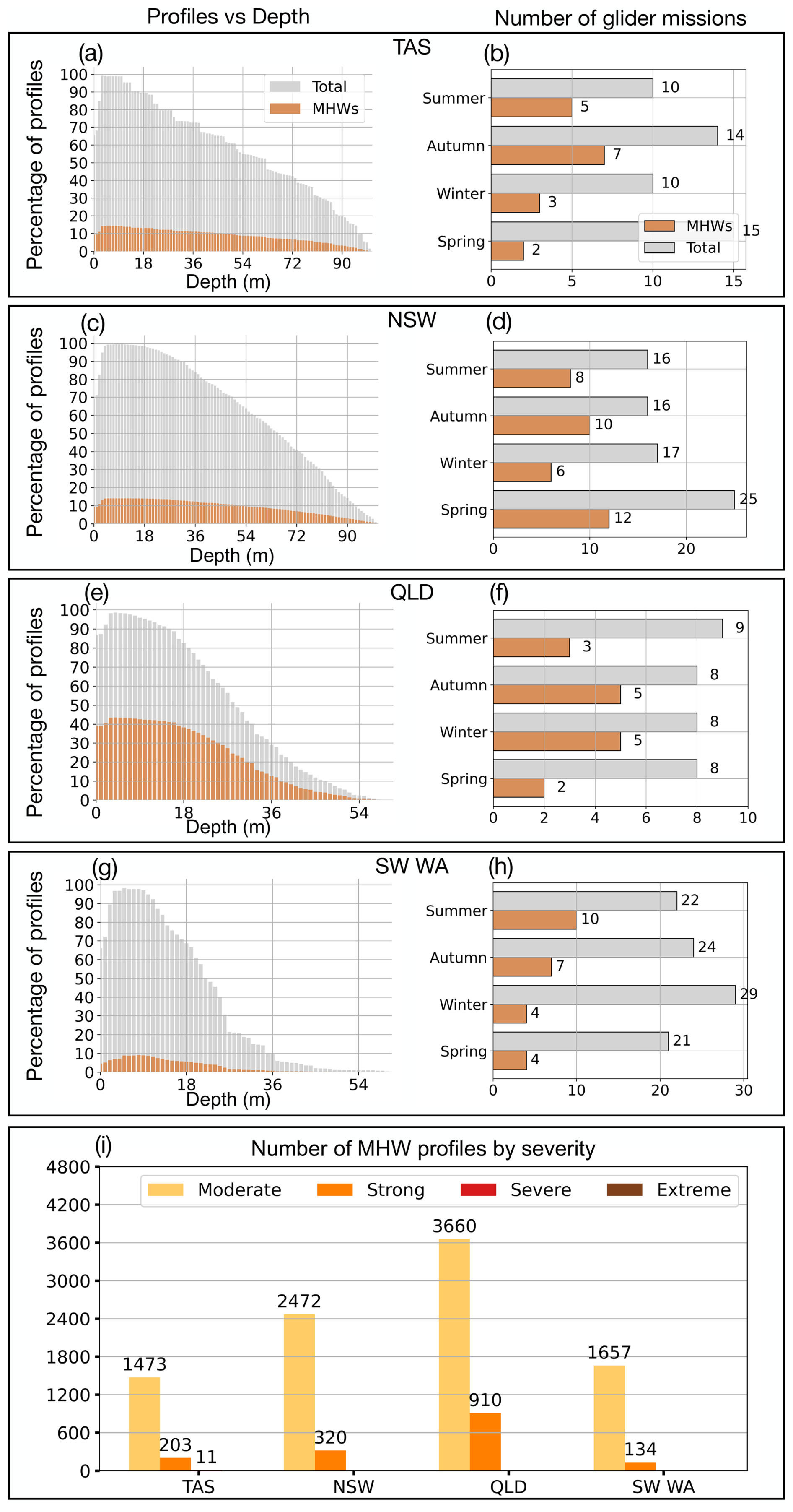
Figure 2 (a, c, e, g) Depth distribution of profiles for Tasmania (TAS), New South Wales (NSW), Queensland (QLD) and southwest Western Australia (SW WA), showing the percentage of total profiles (grey) and MHW profiles (orange) at each depth. (b, d, f, h) Seasonal counts of glider missions for each region, with total missions in grey and MHW missions in orange. (i) Number of MHW profiles per region, classified by severity: moderate, strong, severe and extreme. A glider is classified as being in a MHW based on its position and whether a surface MHW was identified there from the NOAA CoralTemp v3.1 SST with a reference period of 1985–2014.

NSW recorded the greatest number of MHW missions, with 12 separate glider deployments encountering MHW conditions in spring and 10 in autumn (Fig. 2d), corresponding to 1167 and 989 MHW profiles, respectively (Table 1). In SW WA, most missions and profiles occurred in winter and autumn, yet MHW missions (profiles) were more frequent in summer (10 MHW gliders; 953 MHW profiles) and autumn (7 MHW gliders; 512 MHW profiles) (Fig. 2h, Table 1). TAS also recorded the highest number of MHW profiles in autumn (1007 profiles, over 7 missions) and summer (499 profiles, over 5 missions) (Fig. 2b, Table 1). In contrast, QLD showed missions with a more even seasonal spread (Fig. 2f, Table 1), with MHW gliders and profiles more common in winter (5 missions; 894 profiles) and autumn (5 missions; 2269 profiles), this last season being the greatest number of MHW profiles among all seasons and regions. Despite an overall lower number of MHW missions in QLD, the proportion of MHW profiles relative to the total profiles was higher compared to other regions (Fig. 2e, g, Table 1). This reflects the fact that MHWs in QLD are longer-lasting (Fig. 3g), and therefore glider deployments are more likely to capture them.

The vertical distribution of glider profiles also varied across regions due to distinct sloping topography (Fig. 2a, c, e, g), with the highest profile density extending to depths of up to 100 m off TAS and NSW, while profiles were generally shallower (mostly less than 60 m) off QLD and SW WA. MHW profiles, although consistently fewer than non-MHW profiles, were more frequent in the upper 20 m (Fig. 2a, c, e, g) than at the surface or at deeper layers. To ensure a robust representation of the vertical structure, profiles were truncated at depths where less than 10 % of profiles were available (and 20 % for QLD and SW WA), resulting in a maximum analysed depth of 90 m for NSW and TAS, 40 m for QLD, and 30 m for SW WA.

The severity of MHW profiles further highlighted regional differences (Fig. 2i). Most events were classified as Category 1 (“Moderate”), with the highest numbers recorded in QLD (3660 profiles) and NSW (2472 profiles). Category 2 (“Strong”) MHWs were most frequently sampled off QLD with 910 profiles, followed by 320 profiles off NSW, 203 profiles off TAS, and 134 profiles off SW WA. Category 3 (“Severe”) events were few and only sampled off TAS (11 profiles), while Category 4 (“Extreme”) events were not sampled over the continental shelf after quality control steps. Together, these patterns reflect regional contrasts in the number of glider missions, the seasonal and vertical distribution of profiles, and the severity of MHW conditions observed.

3 Results

3.1 Characteristics of surface marine heatwaves

Regional variations in surface MHW metrics derived from satellite SST are illustrated in Fig. 3. From 2009 to mid-2025, the eastern TAS region experienced over 80 surface MHWs (Fig. 3a), whereas fewer than 40 events were detected along the continental shelf. Around Storm Bay in southeast TAS (43° S, 147.5° E), where most gliders were initially deployed, MHWs were generally long-lasting with mean durations of 27–31 d and mean severity exceeding 1.80 (Fig. 3e, i). To better capture the temporal distribution of MHWs relative to glider sampling, a timeline analysis was performed for each region (Fig. 4). MHWs in the TAS region were most frequent from November through to April, with strong to severe events concentrated between January and February (Fig. 4a). In several instances, glider profiles sampled prolonged, strong to severe (Fig. 2i) MHWs, with severity indices exceeding 3, including April 2016, and December 2023 (Fig. 4a).

Relative to other Australian regions, NSW exhibited the highest occurrence of MHWs, with more than 100 MHWs detected over the study period (Fig. 3b). This highly dynamic region is typically characterised by short-lived MHWs lasting less than 10 d (Fig. 3f). On the continental shelf, the mean severity of MHWs in NSW did not exceed 1.65, which is lower than that observed off TAS. However, two short-lived but severe events in September 2013, and October 2018 (Fig. 4b), exceeded a severity index of 3. Glider missions deployed during these periods sampled through the tail of the events, capturing a maximum severity value of 2.1 and 1.6, respectively.

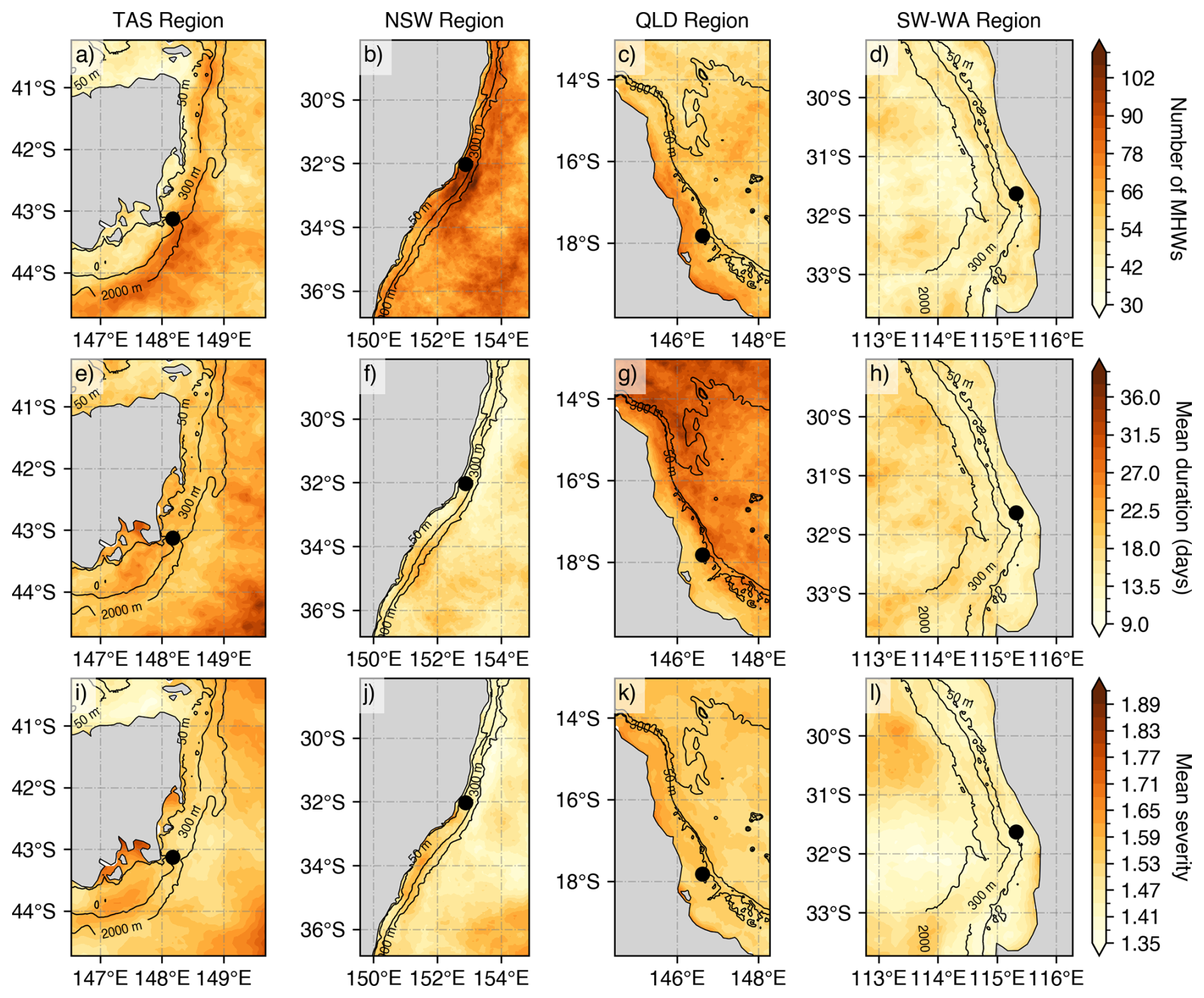
Figure 3 Mean surface MHW metrics based on NOAA CoralTemp v3.1 (climatology 1985–2014 reference period) over the gliders' deployment period (1 January 2009–30 June 2025) by regions: (a, e, i) eastern Tasmania (TAS), (b, f, j) southeastern Australia (New South Wales, NSW), (c, g, k) Queensland region (QLD), and (d, h, l) southwest Western Australia (SW WA). The top panels represent the number of MHWs, the middle panels show the mean duration (in days), and bottom panels indicate the mean MHW severity. MHW severity values are calculated from selected SST pixels (black point) representative of the glider study regions off TAS (148.175° E, 43.125° S), NSW (152.575° E, 32.025° S), QLD (146.625° E, 17.825° S) and SW WA (115.325° E, 31.625° S).

Off northeast Australia (north of 20° S), MHWs were more frequent over the continental shelf, with 66–78 occurrences recorded, compared to fewer events in offshore waters (waters deeper than 200–300 m isobaths Fig. 3c). MHWs on the continental shelf were shorter in duration (Fig. 3g), whereas offshore events were generally more prolonged, lasting 28–36 d on average. Across the central to northern Great Barrier Reef (GBR) off QLD, the severity of MHWs typically had mean values below 1.65. However, there have been events with longer duration and higher severity over the continental shelf, particularly between autumn and winter, in the past decade (Fig. 4c; Benthuysen et al., 2021). These intense seasonal events also coincided with a higher proportion of MHW gliders during these seasons (Fig. 2g). The 2016 MHW stood out as a prolonged (more than 5 months) and strong event captured by three glider missions that sampled the onset (maximum severity: 2.6), middle (maximum severity: 2.3) and tail (maximum severity: 2.6) of the event. Additional strong MHWs were also sampled in March 2017 (maximum severity: 2.9) and September 2022 (maximum severity: 2.1). It is important to note that while some deployments shown in Fig. 4 coincided with severe satellite-detected MHWs, several profiles were excluded during quality control, and therefore may not fully reflect peak severity of the event.

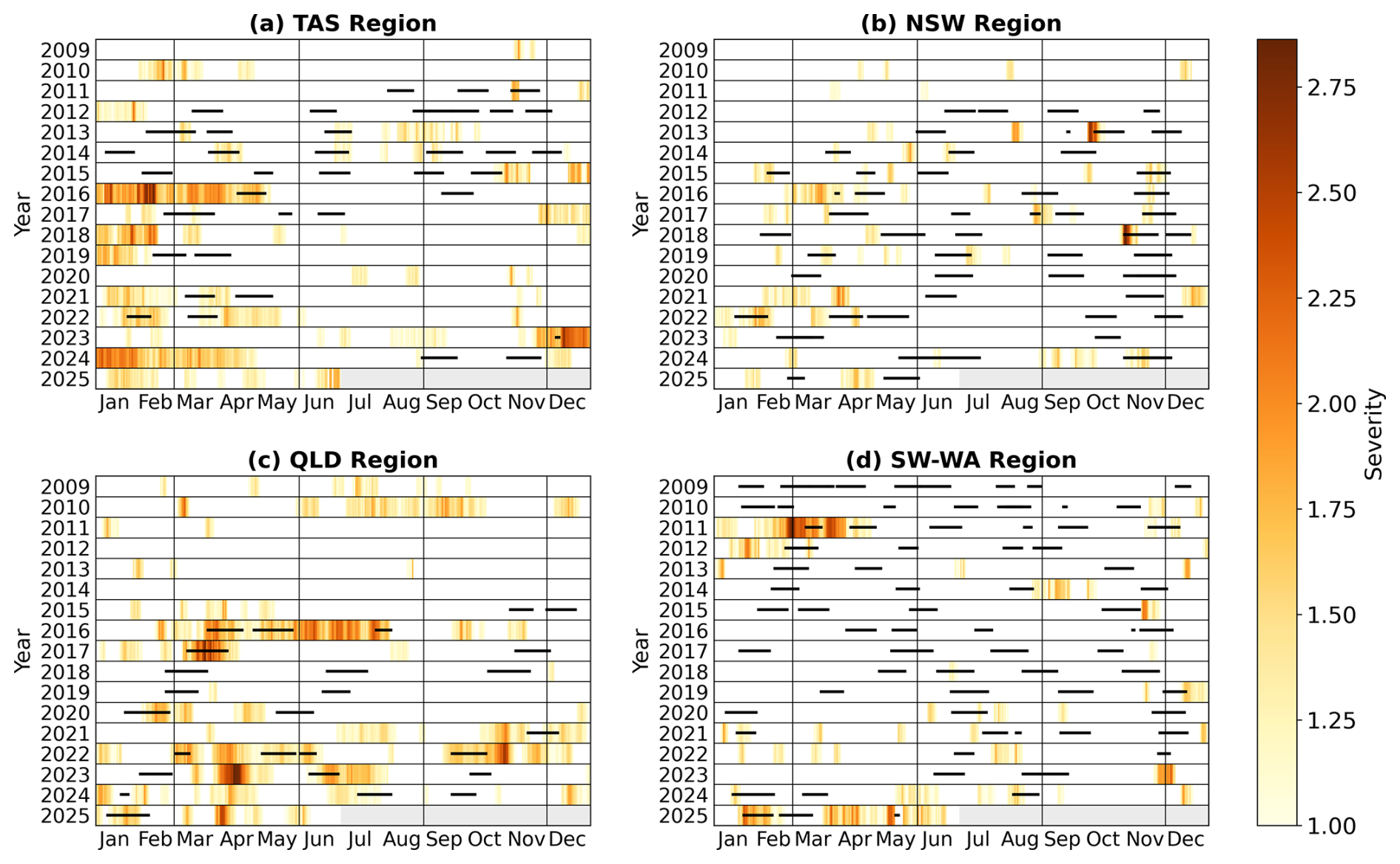
Figure 4 Occurrence and severity of MHWs from January 2009 to June 2025 for (a) Tasmania (TAS), (b) New South Wales (NSW), (c) Queensland (QLD) and (d) southwest Western Australia (SW WA), with horizontal black lines indicating periods when glider missions occurred. Light gray bars in 2025 indicate times beyond the study period. Vertical grey lines delineate seasons.

In contrast to eastern Australia, MHWs off the SW WA were shorter (less than 10 d on average; Fig. 3h), less frequent with less than 45 MHWs recorded (Fig. 3d) and generally weaker in severity ranging between 1.3–1.5 (Fig. 3l). The low severity of MHWs in SW WA appears to be influenced by periods of sustained MHW cold spells off the west coast, which contributed to the lower mean values over the study period (Feng et al., 2021). Such prolonged and cold events can dampen the long-term mean MHW metrics, while other regions in eastern Australia experience a higher prevalence of MHWs with greater duration and intensity. As indicated by the number of glider missions and MHW profiles (Fig. 2h and Table 1), events in SW WA were more frequent and severe between summer and autumn (Fig. 4d). While routine missions are conducted throughout the year, targeted MHW deployments are more likely to occur during summer and autumn, when ocean temperatures are highest and MHW risk is elevated. Increased glider sampling efforts may contribute to increased in situ observations of MHWs during these seasons, although the seasonal peak in MHWs is also evident in the satellite record (Fig. 4d), indicating that the pattern is not only due to sampling effort. The prolonged 2011 MHW is a key event in the region marked by strong to extreme severity nearshore. This event was sampled by two glider missions, one in March (maximum severity: 2.1) and the other in April (maximum severity: 1.6). More recently, in early 2025, SW WA experienced another prolonged, moderate to strong MHW in the region which was also sampled by two glider missions at two critical stages: during the peak (maximum severity: 2.2) and decline (maximum severity: 1.4) of the event, capturing the different phases of the event.

These glider observations were critical, not only in validating satellite-derived MHW metrics across regions and seasons, but also in offering detailed subsurface insights beyond satellite capabilities.

3.2 Marine heatwave severity influences on chlorophyll concentrations and dissolved oxygen

This section examines the impact of surface MHW severity on both surface and subsurface changes in chlorophyll concentrations and DO levels from glider-sampled MHWs over the Australian continental shelf. Figure 5 compares the probability density functions of chlorophyll and DO between non-MHW periods and MHW categories (moderate and strong), above and below the MLD, combining data across all regions. Above the MLD, non-MHWs display a broader chlorophyll fluorescence distribution compared to MHWs, whereas below the MLD, the probability distributions show minimal variations. DO, on the other hand, shows distinct shifts in probability densities under MHW conditions, with multimodal peaks apparent both within and below the MLD, reflecting underlying regional and seasonal variations.

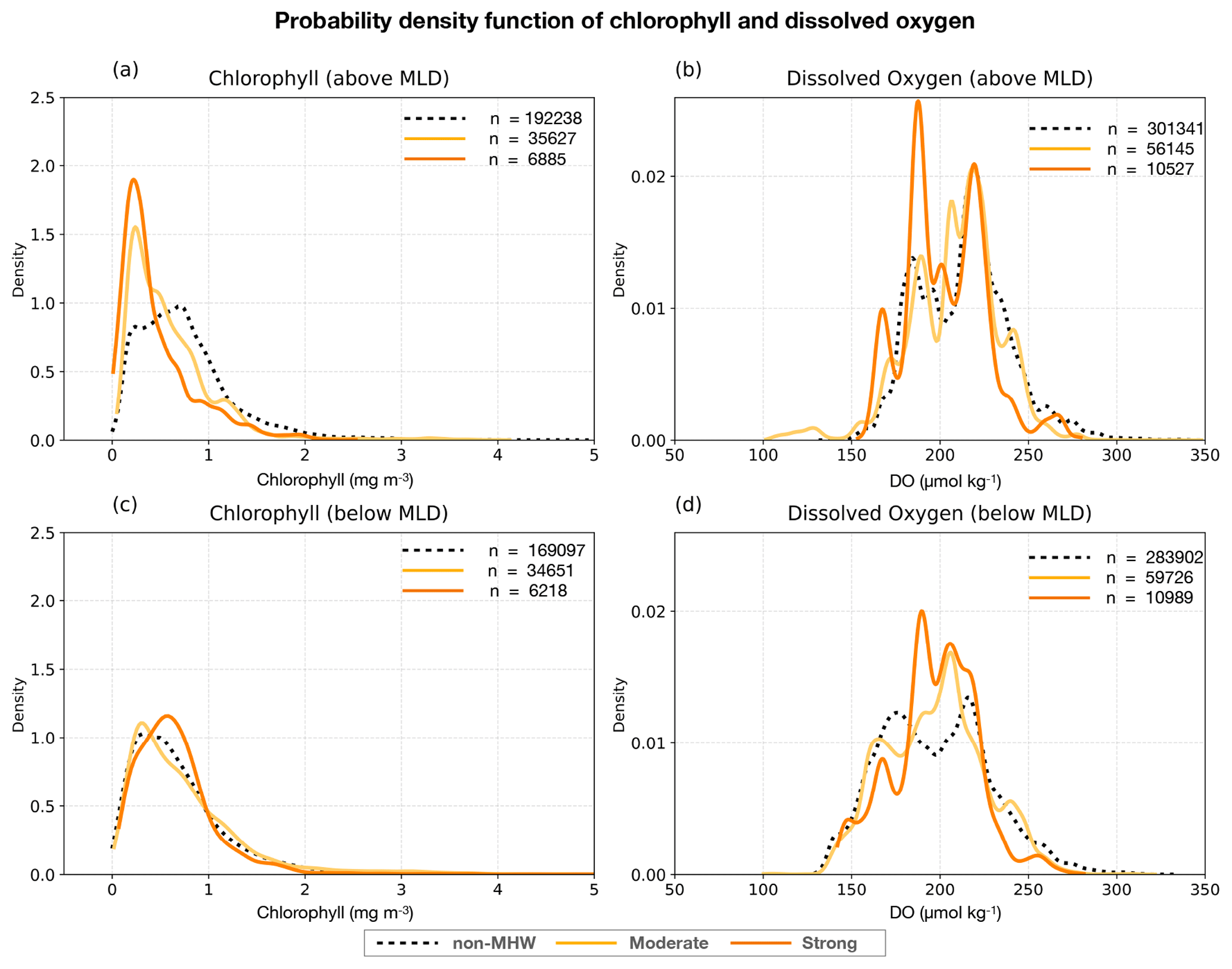
Figure 5 Probability density function of (a, c) chlorophyll fluorescence (mg m⁻³) and (b, d) dissolved oxygen (µmol kg⁻¹) above and below the MLD respectively, during MHWs (thick lines) and non-MHWs (dashed lines) for all regions. The distribution of chlorophyll and dissolved oxygen during MHWs are shown with severity index (S) categories: $\mathrm{1}<S\leqq \mathrm{2}$ (Category 1: moderate; yellow curve), and $\mathrm{2}<S\leqq \mathrm{3}$ (Category 2: strong; orange curve), while non-MHW ones are in black (S ≦ 1; dashed curve). The number of samples (n) are indicated.

Within the mixed layer, chlorophyll concentrations generally decrease during MHWs (Fig. 5a; thick curves) compared to non-MHW conditions. Non-MHW conditions show a peak around 0.7 mg m⁻³, whereas moderate MHWs peak near 0.25 mg m⁻³, and strong MHWs around 0.23 mg m⁻³, indicating progressively stronger decrease of chlorophyll concentrations in the MLD under increasing MHW severity. Below the MLD, non-MHW conditions show lower subsurface chlorophyll (∼ 0.25 mg m⁻³) compared to within the mixed layer, with a slightly more right-skewed distribution (dashed black; Fig. 5c). Moderate MHWs (yellow curve) do not show a significant change in subsurface chlorophyll (∼ 0.25 mg m⁻³) from non-MHWs. In contrast, strong MHWs exhibit a peak around 0.6 mg m⁻³ (orange curve; Fig. 5c), reflecting elevated subsurface concentrations.

For DO above the MLD, non-MHW periods show a bimodal distribution with the two main peaks at approximately 180 and 220 µmol kg⁻¹, suggesting the presence of two types of oxygen regimes (Fig. 5b). The first peak near 220 µmol kg⁻¹ remains stable across non-MHW, moderate and strong severity. Under strong MHWs, the multi-modal structure remains, but the density between 185–195 µmol kg⁻¹ is enhanced relative to non-MHW conditions, while density above 230 µmol kg⁻¹ is reduced. Additionally, a third peak appears near 165 µmol kg⁻¹ during strong MHWs, which may reflect localized depletion of DO. These changes indicate that strong MHWs alter the structure of DO distribution above the MLD, indicating that strong MHWs are associated with a higher frequency of low-oxygen values above the MLD and a relative reduction of high-oxygen values, although the multi-modal structure largely reflects regional and seasonal regimes. As shown in Fig. S2, spring and summer exhibit generally higher mixed layer DO compared to autumn, particularly in TAS and NSW, contributing to higher DO peak (∼ 220 µmol kg⁻¹). In contrast, QLD, which has the largest number of MHW profiles (Fig. 2i), tends to show lower mixed layer DO (Fig. S2), contributing more strongly to intermediate and lower DO density ranges.

For DO below the MLD (Fig. 5d), the distributions slightly shift toward lower oxygen values under all conditions compared to the layer above. During non-MHW periods, two peaks are observed at approximately 175 and 215 µmol kg⁻¹. Under moderate MHWs, the distribution collapses into a single dominant peak near ∼ 205 µmol kg⁻¹, indicating a homogenization of oxygen conditions below the MLD. Strong MHWs display an elevated lower peak at 180 µmol kg⁻¹, similar to above the MLD, and a slightly reduced higher peak around 205 µmol kg⁻¹. Overall, the response of DO to the severity of MHWs appears more heterogeneous than the response in chlorophyll, and does not follow a uniform leftward shift.

Given that the results combine all regions and seasons, they may mask important regional and seasonal differences, as well as sampling compositions. The following sections analyse the vertical profiles of surface MHWs across study regions and seasons to better understand their subsurface impacts on biogeochemical variables.

3.3 Regional and seasonal changes in the water column

The vertical temperature structure of surface MHWs provides insight into how these events penetrate below the surface and interact with stratification and the mixed layer. These physical changes in the MLD, stratification, and MHW depth extent provide the context for examining chlorophyll variations throughout the water column and for assessing the depth of the DCM in particular seasons and regions. Changes in stratification directly affect phytoplankton productivity and oxygen concentrations, making it important to investigate how DO responds to MHWs alongside chlorophyll. In general, DO is highest at the surface due to diffusion from the atmosphere, decreasing with depth, and also varies with temperature through solubility. This vertical perspective sets the stage for comparing regional and seasonal patterns, to assess whether chlorophyll and DO responses to MHWs are consistent across Australia's continental shelf and how they are shaped by local seasonal oceanographic conditions (Figs. 6–9).

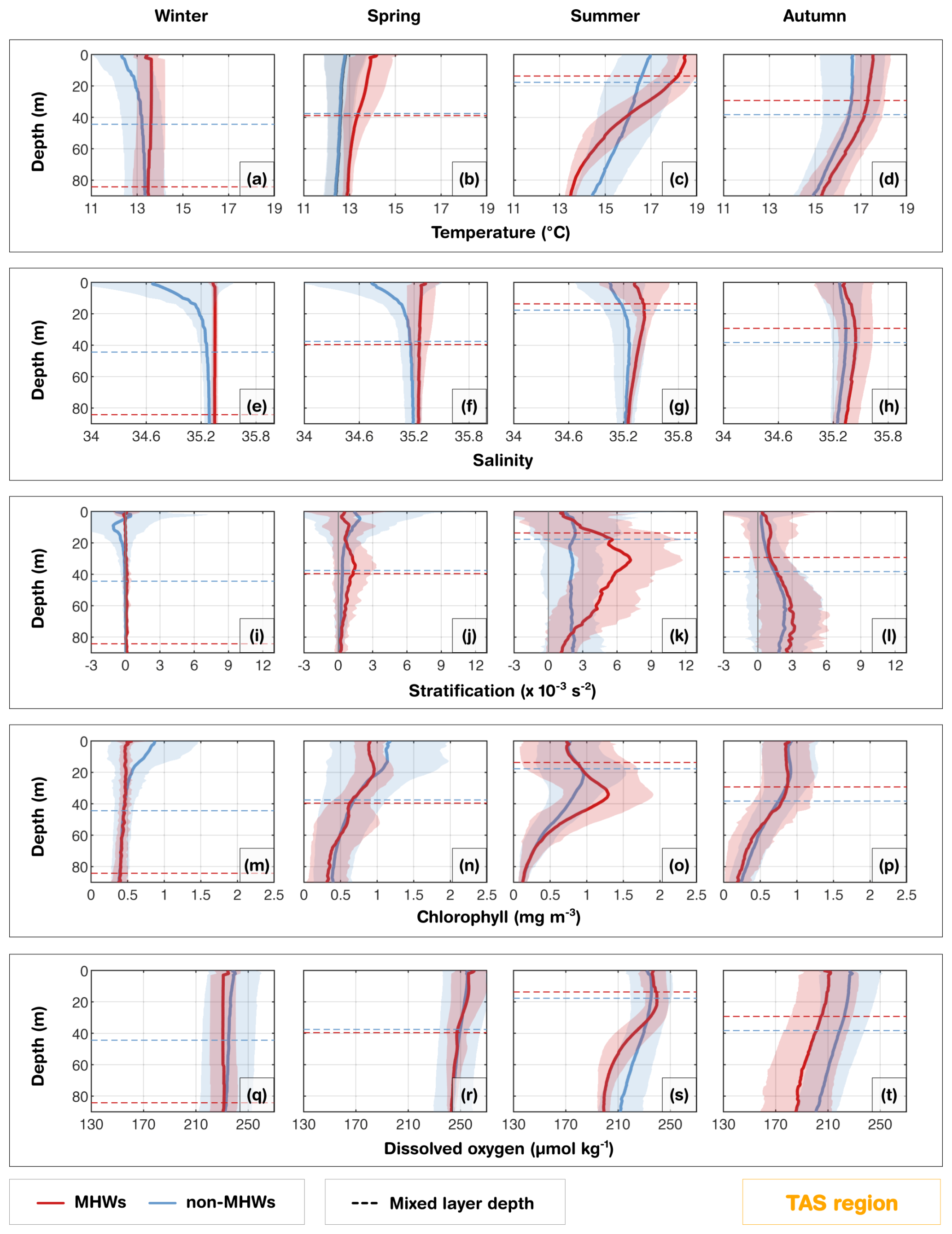
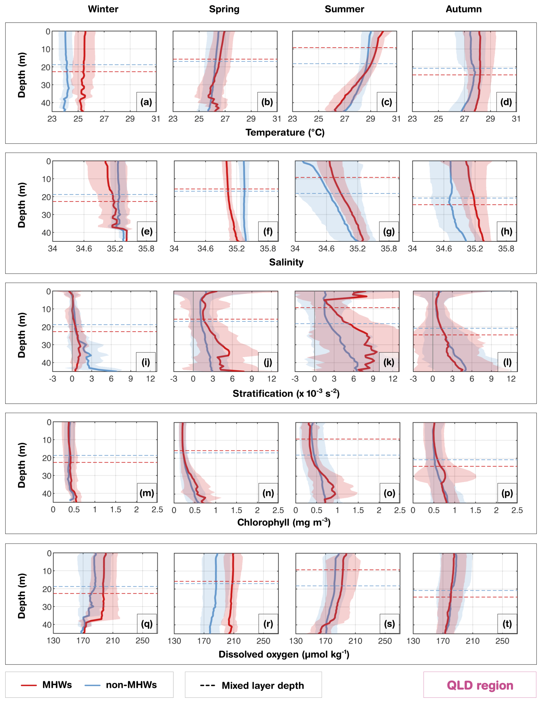
Figure 6 Tasmania region (TAS): Seasonal composite mean profiles of (a–d) temperature (°C), (e–h) salinity (PSU), (i–l) stratification ($\times {\mathrm{10}}^{-\mathrm{3}}$ s⁻²), (m–p) chlorophyll (mg m⁻³) and (q–t) dissolved oxygen (µmol kg⁻¹) averaged for all MHW events (red) and non-MHW events (blue). Horizontal dashed lines indicate the corresponding seasonal composite mean MLDs for MHWs and non-MHWs. Shaded areas represent the respective standard deviations. Seasons are defined as winter (June–August), spring (September–November), summer (December–February), and autumn (March–May).

3.3.1 Eastern Tasmania region: eddy-rich and a convergence zone

Waters off eastern Tasmania (TAS) experience the convergence of warm, salty, and nutrient-poor subtropical waters from the southern extension of the East Australian Current (EAC) and cooler sub-Antarctic waters which lead to complex oceanographic conditions along the continental shelf. The intensification and southward extension of the EAC in the last few decades, associated with changes in the wind stress curl (Hill et al., 2008) and downstream propagating mesoscale eddies (Stammer et al., 2006), has altered stratification and vertical mixing (Holbrook and Bindoff, 1997; Ridgway, 2007; Oliver et al., 2017; Chiswell, 2023). This EAC extension and presence of eddies can, in fact, induce MHWs and have implications for biogeochemical processes and overall ecosystem functioning (Zhao et al., 2022; Chiswell, 2023). From the glider observations, the vertical structure of temperature, salinity, chlorophyll and DO varied strongly within the seasons (Fig. 6). In the TAS region, glider profiles extended down to about 90 m and showed pronounced seasonal cycles in MLD and MHW depth extent. During summer MHWs, the MLD shoaled to about 18 m in summer (Fig. 6c), shallower than the seasonal composite mean MLD of non-MHWs, but extended to the bottom of the water column in winter (Fig. 6a). A similar pattern was reflected in the MHW depth extent, which decreased to about 27 m in summer (Fig. S7) and deepened substantially in the other seasons (∼ 66 m in spring; ∼ 44 m in winter and autumn; using method D in Fig. S7). The pronounced seasonality corresponded to variations in stratification, which peaked at about 7 × 10⁻³ s⁻² near 30 m during summer (Fig. 6k), but was nearly absent in winter (Fig. 6i) and weakly stratifies in spring and autumn (Fig. 6j, l). Meanwhile, salinity values were consistently higher during MHWs all year round and throughout the water column compared to the seasonal mean composites derived from non-MHW conditions (Fig. 6e–h). This indicates that during MHWs, the shelf is influenced by warmer, saltier subtropical water masses associated with a strengthened or southward-shifted EAC, similar to conditions observed during the 2015/2016 Tasman Sea MHW (Oliver et al., 2017). The increased presence of these waters enhances upper-ocean density stratification, particularly in summer, which inhibits vertical mixing with the cooler, fresher sub-Antarctic waters. This is in agreement with the strong and statistically significant correlation (r= 0.94; Fig. 10) observed between MHW depth extent and the depth of maximum stratification during summer in TAS region.

Summer MHWs were marked by reduced chlorophyll at the surface relative to the seasonal composites during non-MHWs in the mixed layer (upper 20 m) but enhanced values at 40 m, exceeding 1.2 mg m⁻³ (Fig. 6o). During summer, the deepening of the DCM corresponded closely to the MHW depth extent and the depth of maximum stratification (r= 0.40; Fig. 10). In other seasons, weaker stratification limited the development of strong DCMs both during MHWs and under non-MHWs conditions. The MHW profile of DO in summer (Fig. 6s) showed a slightly higher concentration in the upper 35 m relative to the seasonal composite mean profile of non-MHWs, exceeding 100 % saturation within this layer (Fig. S3). This suggests enhanced oxygen production in the mixed layer during MHWs, consistent with the strong DCM through photosynthesis (Fig. S3). Similarly, in spring, MHWs showed slightly higher DO and saturation levels (> 100 %) in the upper 25 m than under non-MHW conditions, despite reduced chlorophyll. This suggests that oxygen variability was not controlled by phytoplankton biomass but rather reflected supersaturation due to ventilation. In contrast, during autumn and winter, the oxygen saturation level during MHWs was consistently lower than non-MHW conditions throughout the water column due to weak stratification and reduced DCM, or through solubility loss due to warming (Fig. S3), all of which limit phytoplankton productivity and oxygen production.

3.3.2 New South Wales region: narrow shelf and boundary current influence

In the New South Wales (NSW) region, the narrow continental shelf waters are shaped by the warm EAC, which contributes to mixing and transports warm nutrient-poor waters onto the shelf when it meanders or shifts inshore. The intrusions of the EAC increases the likelihood of full-depth extended MHWs, which are longer than surface restricted MHWs, and dominant in winter (Schaeffer et al., 2023). In this region, seasonal winds and stratification also strongly influence MHWs' depth structure and development, especially in summer (Schaeffer and Roughan, 2017). In the glider observations, during MHWs, warm anomalies were confined to slightly shallower depths (∼ 35 m; Fig. S7) in winter and (∼ 33 m; Fig. S7) autumn, compared to deeper depths in austral summer (∼ 47 m; Fig. S7) and spring (∼ 46 m; Fig. S7). Salinity showed no significant change during MHWs and remained relatively stable throughout the water column throughout the year (Fig. 7e–h). Although waters off NSW are generally more stratified in summer than winter, stratification further intensified and deepened during MHWs in all seasons, reaching ∼ 12 × 10⁻³ s⁻² at 30–40 m in summer and ∼ 3 × 10⁻³ s⁻² at 45 m in winter, closely matching the depth extent of MHWs (Figs. 7i, k, S7, 10).

Figure 7 Same as Fig. 6, but for the New South Wales (NSW) region.

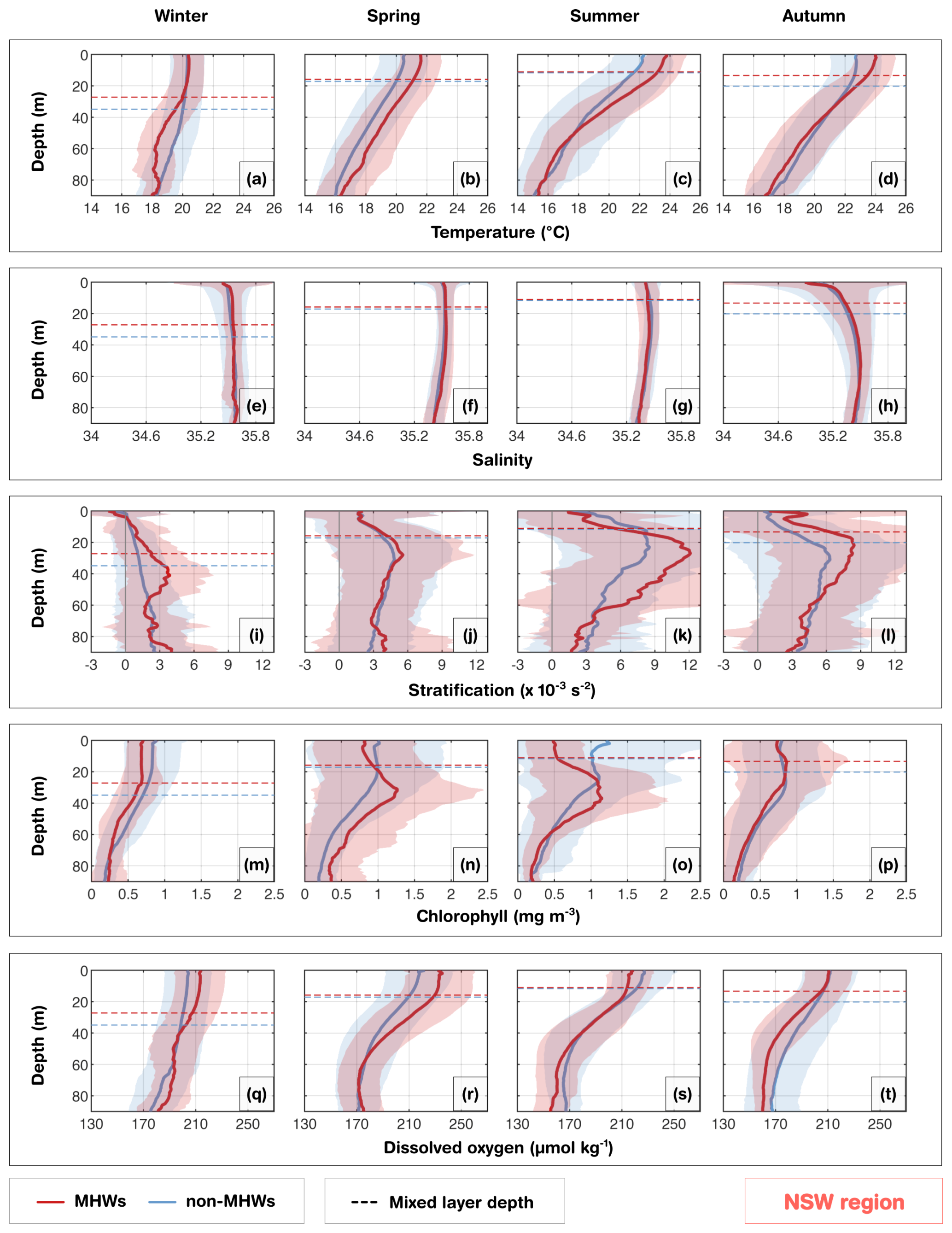
The DCM experienced strong seasonality. Across all seasons, surface chlorophyll concentrations were reduced during MHWs, while increasing at ∼ 20–40 m (exceeding 1 mg m⁻³) during spring, summer and autumn (Fig. 7n–p). These chlorophyll maxima were deeper and stronger than under non-MHW conditions, and their depth aligned well with both maximum stratification and the MHW depth extent (Fig. S7). In contrast, during winter, weaker stratification corresponded to shallower or absent DCMs, with chlorophyll concentrations below 1 mg m⁻³ (Fig. 7m).

In summer, MHWs were associated with reduced DO in the upper 20 m, likely due to warming-induced reduced solubility (Fig. S3). At intermediate depths, a more pronounced DCM was present (Fig. 7o). Further deoxygenation below 50 m may result from enhanced respiration of sinking organic matter from the intermediate layer. However, little difference in DO levels from non-MHW conditions in the intermediate layer indicated that photosynthesis was insufficient to alter the total mean DO (Fig. S3). Conversely, in spring, MHWs were associated with higher DO concentrations in the upper 50 m, exceeding 100 % saturation relative to non-MHW conditions within the mixed layer (Fig. S3). This DO enhancement during spring is consistent with strong stratification and deep DCM (Fig. 7j, n, r), and is likely driven by photosynthesis, mixing or advection of oxygen-rich waters. By contrast, in autumn, DO concentrations were similar within the mixed layer but decreased below the MLD (Fig. 7t), consistent with a DCM positioned higher in the water column (Fig. 7l).

3.3.3 Queensland region: shallow shelf and biologically active area

The Queensland (QLD) region is home to the GBR, which has a shallow continental shelf with coral reefs and reef passages and the shelf circulation is influenced by the Gulf of Papua Current (in the north), East Australian Current (EAC; from the central sector to south), the Coral Sea circulation, riverine inputs and wind-driven processes (Ridgway et al., 2018; Benthuysen et al., 2022; Wolanski and Kingsford, 2024). The seasonal composite mean of MLD and the MHW depth extent largely followed the seasonal cycle (Figs. 8, S7). During summer MHWs, the MLD shoaled to 9 m consistent with a shallow MHW depth extent (∼ 19 m; Fig. S7), and strong stratification peaking above 9 × 10⁻³ s⁻² at the surface (Fig. 8k). The intense near-surface stratification is likely exacerbated by the formation of barrier layers during the wet season (Schroeder et al., 2012), where riverine freshwater input and precipitation create a buoyant low-salinity lens (Fig. 8g) and subsurface intrusive upwelling through reef passages brings saltier Coral Sea waters below (Benthuysen et al., 2016). These barrier layers inhibit vertical mixing, effectively trapping heat in the surface layer and intensifying the MHW magnitude. In contrast, during winter and autumn MHWs, the MLD deepened to 23 and 25 m respectively, consistent with a deepening of the MHW depth extent to about 22 and 27 m respectively (Fig. S7). During these seasons, the stratification weakened to less than 3 × 10⁻³ s⁻². Although fresher waters were observed near the surface in winter and spring, salinity values were not as low as in summer, and the vertical salinity gradient was not as pronounced as in summer and autumn, suggesting the dominance of wind-driven and convective mixing in homogenizing the water column during these cooler seasons.

Figure 8 Same as Fig. 6, but for the Queensland (QLD) region.

Biologically, the strong physical stratification during summer MHWs shaped the vertical chlorophyll structure. The DCM reached 1 mg m⁻³ at 40 m (Fig. 8o), coinciding with strong fluctuations in stratification levels below 30 m, acting as a productive interface where light and nutrient availability overlap. Although less pronounced than summer, autumn also displayed high chlorophyll concentrations exceeding 0.9 mg m⁻³ at 30 m. However, chlorophyll concentration during MHWs in the upper 20 m remained lower than the seasonal composites, indicating reduced productivity in the upper layers. The increased chlorophyll pattern observed in the subsurface layer may reflect the seasonal transition toward weaker stratification and associated nutrient entrainment sustaining subsurface productivity from deeper waters during the autumn MHWs. In contrast, winter and spring MHWs showed a weaker coupling between stratification and chlorophyll than the other seasons, consistent with enhanced mixing. The DO during MHWs compared to non-MHW conditions were consistently higher throughout the shallow water column (except in autumn). This presents a counterintuitive thermodynamic behaviour, as warmer water typically holds less dissolved gas. Consequently, the observed DO increase during summer, and spring indicates that biological oxygen production (photosynthesis) was sufficient to offset the physical solubility loss induced by warming (Fig. S3). While biological production dominates the summer signal, the higher DO observed during MHWs in winter may be related to seasonal ventilation that drives the deep vertical extent of temperature anomalies, leading to higher oxygen levels than normal. In contrast, the lower DO levels in autumn, despite the presence of subsurface chlorophyll, appears to be dominated by enhanced respiration rates, consuming oxygen as organic matter from prior blooms. In addition to enhanced respiration, reduced nutrient availability following summer could limit primary production, thereby decreasing oxygen supply.

3.3.4 Southwest Western Australia region: shallow shelf and oligotrophic conditions

The southwest Western Australia (SW WA) region is characterised by a shallow shelf dominated by the warm, fresh poleward-flowing Leeuwin Current, maintaining oligotrophic conditions, while the Capes Current emerges inshore during spring and summer months with upwelling leading to phytoplankton blooms (Hanson et al., 2005; Feng et al., 2025). The gliders were sampled over this coastal region, where the shelf narrows from ∼ 50 to 20 km (Fig. 1e; Brooke et al., 2010). From the coast to the mid-shelf, waters had weaker stratification in the upper 40 m (Fig. 9i–k) compared with other regions, where the small temperature inversion in autumn and winter is consistent with an annual climatology from nearby mooring measurements (Feng et al., 2025). Unlike the stratified systems in eastern Australia, this weak stratification coupled with the dominance of the Leeuwin Current drives downwelling-favorable conditions that facilitate the rapid vertical propagation of surface heat anomalies. As a result, during surface MHWs, anomalously warm surface temperatures extended further deep in all seasons, following the seasonal cycle of the MLD, leading to ∼ +1–2 °C differences in the mean temperature profiles compared with non-MHW conditions (Fig. 9a–d). The MLD shoaled during summer MHWs compared to non-MHW conditions, in contrast to a deepening during winter MHWs. In autumn, the MHW conditions were warmer and fresher than non-MHWs, potentially in part related to sampling during the 2011 Ningaloo Niño (Fig. 4d), when glider measurements were concentrated around 31.5–32° S. During this extreme event, low salinity anomalies were transported by the Leeuwin Current and were some of the lowest recorded values since the 1950s (Feng et al., 2015). This highlights that severe MHWs in this region are largely advection-driven events, where the transport of buoyant, low-salinity tropical waters enhances the density contrast with offshore waters, further trapping heat against the coast.

Figure 9 Same as Fig. 6, but for the southwest Western Australia (SW WA) region.

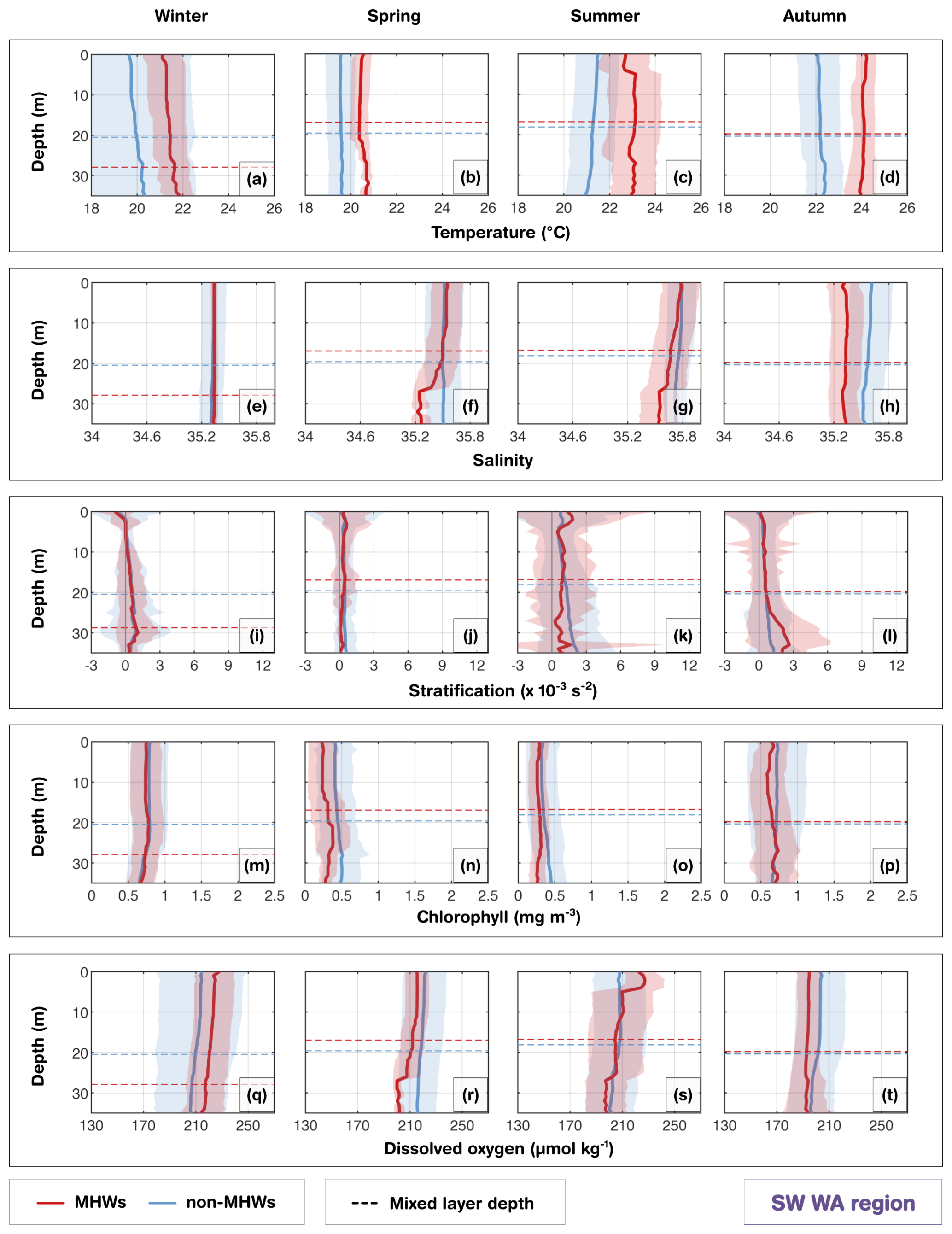
Biogeochemically, the strong advective nature of these MHWs exerts a controlling influence on shelf productivity. During surface MHWs, shelf waters had lower chlorophyll concentrations than non-MHWs (Fig. 9m–p). Surface MHWs were associated with anomalously high oxygen saturation levels (> 100 %; Fig. S3), higher than non-MHW conditions during summer and winter. In summer, this likely reflects biological production in the upper layers due to shallower MLD while in winter, it may be partially influenced by enhanced ventilation (Fig. S3). Weak stratification facilitates this supersaturation by allowing atmospheric oxygen to mix effectively throughout the water column, even if dissolved oxygen is not substantially higher than non-MHW conditions. However, significantly lower DO levels were observed in spring and autumn (Fig. 9r, t). In autumn, with sampling through the 2011 Ningaloo Niño, the relatively reduced near-surface chlorophyll and DO might reflect equatorward influences on this region, as offshore waters to the north have been recorded with lower chlorophyll and DO (e.g. Woo and Pattiaratchi, 2008; Weller et al., 2011). This reduction suggests a decoupling from the solubility-driven pattern seen in other regions, pointing instead to the physical advection of warm, nutrient-poor, and oxygen-depleted tropical waters by the intensified Leeuwin Current, which suppresses local productivity and Capes Current upwelling. These results reveal that, in the upper 40 m of coastal waters off SW WA, reduced stratification influences the vertical structure of chlorophyll and DO (Fig. 10), even during surface MHWs, and they could be affected by latitudinal transport of water properties, as has been found during MHWs caused by a Leeuwin Current intensification.

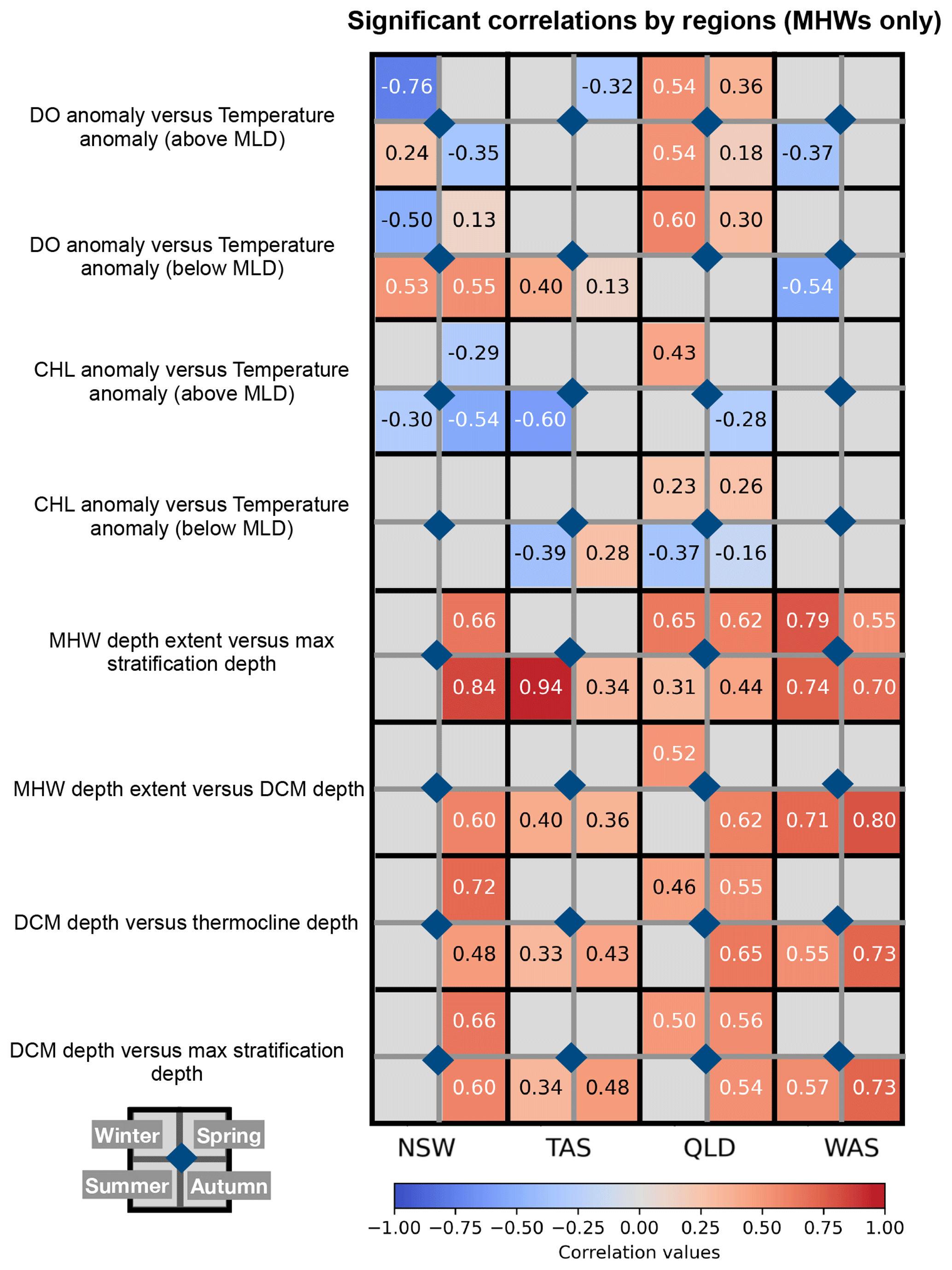
Figure 10 Synthesis figure of seasonal correlations between key physical–biogeochemical variables during MHWs across four regions (NSW, TAS, QLD, SW WA). Rows correspond to variable pairs: (1) dissolved oxygen anomalies (DO) versus temperature anomalies (above the MLD), (2) dissolved oxygen anomalies (DO) versus temperature anomalies (below the MLD), (3) chlorophyll anomalies versus temperature anomalies (above the MLD), (4) chlorophyll anomalies versus temperature anomalies (below the MLD), (5) MHW depth extent versus depth of maximum stratification, (6) MHW depth extent versus DCM depth, (7) DCM depth versus thermocline depth, and (8) DCM depth versus depth of maximum stratification. Columns correspond to regions. Each cell is subdivided into four seasonal quadrants, colored by the Pearson correlation coefficient (r) values with values indicated within each quadrant. Correlation values are in black if magnitude is less than 0.5 and in white if greater than 0.5. Grey cells indicate cases with fewer than 30 sample points or correlations that are not statistically significant (p>0.05).

4 Discussion

MHWs have been extensively documented around Australia, yet their impact on subsurface biogeochemical variables remains a critical gap in our understanding due to limited long-term observations. We used satellite SST and up to 16 years of glider observations across four contrasting and well-observed coastal regions: eastern Tasmania (TAS), New South Wales (NSW), Queensland (QLD), and southwest Western Australia (SW WA). Our study reveals how surface MHWs alter, seasonally, the subsurface temperature, salinity, stratification, and biogeochemical variables (chlorophyll and dissolved oxygen). These findings provide new insights into region-specific responses, which help fill critical gaps in understanding the subsurface impacts of MHWs along the continental shelf of Australia.

Across most regions, the vertical structure of temperature, salinity, and stratification displayed strong seasonality, with shallow mixed layers and enhanced stratification in summer, and deeper, weaker stratification in winter. During MHWs, these patterns tend to be intensified, with shallower MLD and stronger stratification in summer, and deeper MLD in winter (except in NSW). During winter MHWs, the water column is already weakly stratified, and warming alone does not generate a strong density gradient to shoal the MLD. In addition, anomalous processes associated with winter MHWs, such as wind-driven mixing and horizontal advection, can further deepen the MLD relative to typical winter conditions. In some regions, such as Western Australia, Leeuwin Current-driven MHWs produce deep warming that can result in a deep MHW structure (Zhang et al., 2023), where warmer water penetrates to greater depths, thereby leading to deeper MLD during MHW winters. In contrast, NSW did not exhibit this deepening of the MLD during winter MHWs due to the hydrography of the EAC which impacts the NSW shelf year-round. Unlike other regions, stratification in NSW is not driven purely by seasonal heating and cooling but is strongly modulated by shelf encroachment of the EAC, mesoscale eddies, and current instabilities. This persistent influence also shapes the seasonality of phytoplankton in NSW, with summer-spring biomass maxima and reduced winter abundance (Armbrecht et al., 2015), consistent with our findings. SW WA exhibited particularly minimal stratification changes due to its naturally well-mixed conditions, however, transient increases in stratification can occur during periods of wind relaxation or fluctuations in the Leeuwin or Capes Currents. The MHW depth extent was shallower in strongly stratified (summer) conditions and deeper during winter when the water column was more homogeneous. These results align well with Schaeffer et al. (2016a) and with hypothesis (3) that the vertical depth extent of surface MHWs vary seasonally according to background stratification and hydrography.

Chlorophyll responses are tightly coupled to MHW severity and regional hydrography. Results showed that surface chlorophyll above the MLD overall declines with increasing MHW severity, in line with previous studies (Le Grix et al., 2021; Sen Gupta et al., 2020; Gruber et al., 2021). This finding supports hypothesis (4) that the severity of MHW modulates chlorophyll concentration and is also consistent with hypothesis (1) that surface MHWs generally reduce chlorophyll concentrations in the mixed layer. The observed decline in surface chlorophyll with increasing severity is likely driven by enhanced stratification and reduced nutrient supply from the subsurface which limit surface phytoplankton growth during MHWs. This pattern is evident in the correlation plots (Figs. 10 and S4), which reveal an overall negative relationship between temperature and chlorophyll anomalies above the MLD, except in SW WA where limited sampling may affect the correlation (Fig. S8).

Subsurface chlorophyll distributions during MHWs has been a topic of incipient discussion. Here, our study showed evidence for increased chlorophyll below the MLD during strong MHWs along the Australian continental shelves, pointing to the formation of a sharper and deeper DCM in spring, summer and autumn due to enhanced stratification (except in the oligotrophic region of Western Australia). This finding supports hypothesis (2), indicating that despite surface reductions, MHWs can promote deeper chlorophyll maxima and enhanced subsurface productivity. Although the surface becomes nutrient-poor, the shoaling of the MLD during MHWs increases phytoplankton exposure to higher light intensities, thereby allowing phytoplankton to thrive at depth (e.g. Hayashida et al., 2020). DCM depth correlated strongly with the depth of maximum stratification in NSW (Pearson correlation coefficient, r= 0.66 in spring, r= 0.60 in autumn), in TAS (r= 0.48 in autumn), in QLD (r= 0.56 in Spring) and SW WA (r= 0.73 in autumn), all statistically significant. We also found strong correlations between DCM depth and MHW depth extent, in NSW (r= 0.60 in autumn), QLD (r= 0.62 in autumn, r= 0.52 in winter) and SW WA (r= 0.71 in summer, r= 0.80 in autumn). This finding is consistent with Ma and Chen (2025), who showed that MHWs promote DCM development at the global scale. In contrast, in winter or in vertically-mixed upper ocean waters, MHWs penetrate to depth, eroding stratification and suppressing DCM. The level of stratification controls the thermocline depth, which we found to be strongly correlated with DCM depth (Figs. 10 and S6), and thereby governs both the vertical position of the DCM and the MHW depth extent. Our results support hypothesis (3) that regional hydrography and seasonal stratification control the vertical extent of MHWs.

DO responses to MHW and their severity are less straightforward. Australia's surrounding waters exhibit distinct oxygen regimes due to contrasting water masses, biogeochemical environments and seasonal variability. Low-oxygen regimes are usually present in tropical and subtropical regions (Paulmier and Ruiz-Pino, 2009; Davila et al., 2023) such as QLD and SW WA, influenced by oxygen-poor water masses, while high-oxygen regimes are found in temperate regions (NSW, TAS), dominated by well-ventilated waters. During strong MHWs, low-oxygen regimes may become further deoxygenated in the MLD (Figs. S2, S3), such as in QLD, due to enhanced stratification and reduced vertical ventilation, consistent with hypothesis (1) that MHWs reduce dissolved oxygen in the mixed layer and hypothesis (4) that MHW severity modulates dissolved oxygen variability. Although reduced upwelling can limit the entrainment of oxygen-poor subsurface waters, it also restricts the supply of oxygen from deeper layers and reduces mixing, isolating the mixed layer. In shallow coastal regions, elevated temperatures further decrease solubility and may increase the biological oxygen demand. Besides temperature's direct effect on oxygen solubility, changes in DO arise from complex interactions between circulation and stratification, and primary productivity (Gruber, 2011; Gruber et al., 2021).

Regional differences in DO distributions during MHWs illustrate these complex interactions due to circulation and stratification, and primary production. In NSW and TAS, MHWs generally decrease DO in the MLD (except summer NSW), consistent with lower oxygen saturation level than during non-MHWs (Fig. S3), due to the temperature-dependent decrease in oxygen solubility (negative DO tendency with temperature in Fig. S5c). However, below the MLD, localized oxygen increases occur particularly in summer, near subsurface chlorophyll maxima (Figs. 10, S5b, d). These seasonal increases may reflect enhanced biological production during which oxygen is generated below the MLD through photosynthesis, or ventilation associated with the strong East Australian Current (EAC) and its eddy-driven intrusions (Malan et al., 2020). In addition to these biophysical drivers, regional wind patterns (Wood et al., 2016) further modulate the vertical structure of DO during spring in NSW.

In QLD, DO responses to MHWs are linked to seasonal changes in stratification, mixing, and biological productivity. During summer MHWs, strong near-surface stratification, reinforced by riverine freshening and wet-season rainfall, creates a shallow MLD that traps heat and supports high biological activity. This results in elevated DO throughout the upper water column, with oxygen saturation exceeding 100 % in the MLD (Fig. S3), indicating that photosynthesis more than compensates for the temperature-driven decline in oxygen solubility. This finding is in agreement with hypothesis (2) that subsurface waters may experience enhanced oxygen concentrations associated with deeper productivity. In contrast, autumn shows lower DO during MHWs compared to non-MHW periods, although subsurface chlorophyll remains elevated. This reduction coincides with warmer and saltier conditions that decrease oxygen solubility and combined with weaker stratification, facilitates the mixing of low-oxygen waters upward. Enhanced respiration following the summer bloom may also deplete DO.

In SW WA, well-mixed waters in the upper 40 m exhibited relatively uniform DO profiles, with enhanced DO in summer and winter oxygenation during MHWs. For example, in summer, the weakened and offshore-displaced Leeuwin Current combined with strong southerly winds (Feng et al., 2025) promotes strong ventilation and enhanced mixing. During autumn, anomalously warm, fresh waters with reduced chlorophyll in the upper 20 m and reduced DO, compared with non-MHW conditions, indicate the potential influence for intensified Leeuwin Current transport to affect biogeochemical variables during advection-driven MHWs (Pearce and Feng, 2013; Benthuysen et al., 2014). Overall, the study results indicate that stratification and primary productivity jointly regulate oxygen variability, with regional hydrography determining whether MHWs enhance or suppress oxygenation across the water column.

While this study provides a comprehensive analysis of subsurface thermal and biogeochemical structure associated with surface MHWs, several limitations related to sampling density should be acknowledged. Despite the availability of 16 years of glider observations, sampling remains uneven across regions, depths and seasons, which constrains the robustness of some composite profiles. In particular, subsurface properties during spring MHWs are not robustly characterised in some regions due to the small number of captured events. For example, TAS in spring are based on only two MHW events, limiting confidence in the seasonal mean of these profiles. Similarly, in QLD, the number of MHW profiles during autumn exceeds that of non-MHW profiles, which may not give a true representation of the seasonal mean.

Additional limitations arise from combining surface MHW detection based on daily, night-time, gap-filled satellite data with sub-daily in situ glider observations, which may bring inconsistencies between both surface and subsurface signals. Furthermore, the available dataset is insufficient to assess the influence of large-scale climate modes on the subsurface structure of surface MHWs, and lack some biological parameters (e.g. nutrient concentrations) which restricts the interpretation of DO and DCM. Addressing these limitations will require high-resolution observations across all seasons and coordinated modelling efforts to develop robust subsurface climatologies.

5 Conclusions

This study shows that the impacts of MHWs on dissolved oxygen and chlorophyll along the Australian continental shelf depend strongly on regional hydrography, seasonal stratification, and, to some extent, event severity. Taken together, our results show that surface-only perspectives underestimate the biogeochemical and potential ecological impacts of MHWs. Subsurface glider observations revealed that MHWs can simultaneously suppress surface productivity while intensifying subsurface production, with consequences for oxygen levels and food-web dynamics, depending on regional hydrography and stratification. Stratification, which appears consistently enhanced during summer MHWs, emerges as a useful proxy for the vertical extent of surface MHWs and on the DCM. These findings underscore the importance of accounting for region-specific monitoring to manage ecological consequences of MHWs.

The interaction between physical processes, such as seasonal circulation, stratification and biological feedback, including deep chlorophyll maxima formation and oxygen production, highlights the complex biogeochemical responses to MHWs. By leveraging up to 16 years of glider observations, this work demonstrates the importance of sustained subsurface monitoring and coupled physical–biogeochemical approaches to better predict ecosystem vulnerability. Future research is needed to transform sparse and high-frequency sampling of continental shelf waters to develop coastal climatologies appropriate for assessing subsurface MHW impacts. Long-term measurements are key to improving our understanding of MHWs' vertical structure, drivers, and ecological consequences and, in combination with shelf modelling, can provide a holistic view of how they affect variability and extremes in our coastal and shelf systems. These efforts are critical for managing the impacts of MHWs on marine ecosystems under a warming climate.