Intraseasonal modulation of sea surface temperatures in the Tropical North Atlantic by African Easterly Waves

The sea surface temperature (SST) variability in the Tropical North Atlantic (TNA) plays a crucial role in the regional climate by modulating the Intertropical Convergence Zone (ITCZ) and influencing precipitation, convective systems, and tropical cyclones. While atmospheric synoptic-scale intraseasonal variability in this region is dominated by African Easterly Waves (AEWs), their impact on SST remains poorly understood. This study investigates the modulation of SST by AEWs using a regional configuration of a coupled ocean-atmosphere model and moored surface buoy air-sea observations. The results reveal a significant AEWs signature in SST anomalies, with typical temperature fluctuations of approximately ±0.3 °C (reaching up to ±0.5 °C for the strongest events). A heat budget analysis shows that AEWs mainly influence SST through modulation of the latent heat flux, shortwave radiation, and vertical mixing. The contribution of ocean mixing and that of the air-sea fluxes appear to be of similar order. The dominant 3–5 d AEWs exhibit a stronger impact than their 6–9 d counterparts. These findings highlight the role of AEWs in driving SST variability and mixed-layer dynamics, underscore the importance of accurately representing them in coupled climate models, and call for further investigation into their influence on the mean and seasonal upper-ocean state.

1 Introduction

The variability of the sea surface temperature (SST) in the Tropical North Atlantic (TNA) is a key factor in determining the regional climate and affects surrounding countries. It plays a critical role in modulating the position of the Intertropical Convergence Zone (ITCZ) (Wane et al., 2021), as shown by the strong correlation between the ITCZ and the regions of highest SST (zonal band of SST≥27 °C) (Graham and Barnett, 1987; Waliser and Graham, 1993; Opoku-Ankomah and Cordery, 1994). This variability plays a key role in establishing and maintaining convective systems and precipitation in the tropical Atlantic, West Africa, and northeastern South America (Moura and Shukla, 1981; Hastenrath and Greischar, 1993; Nobre and Shukla, 1996; Sultan and Janicot, 2000; Nicholson, 2009; Tomaziello et al., 2016). Furthermore, the frequency and intensity of tropical cyclones, which draw their energy from the warm waters of the Tropical Atlantic, are influenced by these SST anomalies (Emanuel, 2005; Webster et al., 2005). Therefore, a better understanding of the mechanisms involved in SST variability is essential not only to enhance our comprehension of climate processes, but also to reduce SST biases in coupled models and refine climate forecasts.

At the synoptic scale, atmospheric variability in this region is predominantly governed by African Easterly Waves (AEWs) (Thompson et al., 1979; Diedhiou et al., 2001). These are westward-propagating atmospheric disturbances with periods ranging from 2 to 10 d, which develop during the boreal summer over the tropical region, primarily across West Africa. AEWs generally originate from atmospheric instabilities, particularly barotropic-baroclinic instabilities associated with the African Easterly Jet (Burpee, 1972). They also originate from convection, which not only facilitates their initiation but can also enhance their growth (Berry and Thorncroft, 2005; Mekonnen et al., 2006; Thorncroft et al., 2008; Russell et al., 2020). AEWs are generally classified into two period bands: 3–5 and 6–9 d (Diedhiou et al., 1998a, b, 1999; Felice et al., 1990, 1993; Wu et al., 2013). The 3–5 d AEWs propagate preferentially on either side of the African Easterly Jet, before merging over the Atlantic, generally at around 17.5° N. They have average-zonal wavelengths of around 3000 km and phase speeds of up to 10 m s⁻¹ (Diedhiou et al., 1998a; Reed et al., 1988; Thorncroft and Hodges, 2001). Those of 6–9 d, further north and more intermittent, unfold with an average phase speed of around 6 m s⁻¹ and wavelengths of around 5000 km (Diedhiou et al., 2010; Wu et al., 2013).

On their trajectory, AEWs interact closely with deep convection, playing a central role in modulating atmospheric dynamics in West Africa. Several studies have highlighted the influence of AEWs on the organization, intensity and propagation of mesoscale convective systems (Berry and Thorncroft, 2005; Kiladis et al., 2006; Russell et al., 2020). In particular, these interactions are manifested by an amplification of convection in cyclonic convergence zones associated with wave troughs, thus promoting the triggering or intensification of precipitation (Fink and Reiner, 2003; Kiladis et al., 2006). Moreover, under certain favorable conditions, particularly when deep convection persists downstream of the wave, these systems can contribute to the cyclogenesis process in the TNA (Thorncroft and Hodges, 2001; Dunkerton et al., 2009; Russell et al., 2017; Bercos-Hickey and Patricola, 2025).

In the Tropical North Pacific, Mickett et al. (2010), using a slab model and comparing surface wind-induced inertial kinetic energy fluxes in the mixed layer, show that these waves (Pacific Easterly Waves, PEWs) resonantly force inertial motions, which influence sea surface temperatures. In their recent work, Hummels et al. (2020) put forward the hypothesis that, in the TNA, AEWs would contribute to cooling the ocean surface, through the associated latent heat fluxes, and the strong vertical mixing at the base of the mixed layer induced by the near-inertial waves they would generate. However, the importance of AEWs in the regional heat balance, and consequently on the surface temperature, remains to be clarified. While numerous studies have investigated the characteristics of AEWs and their role in climate modulation, to our knowledge no study has yet examined their impact on ocean surface conditions in the Tropical Atlantic. Using a coupled ocean–atmosphere configuration of the Tropical Atlantic (Gévaudan et al., 2021), the aim of this study is to examine whether AEWs influence SST in this region and investigate the underlying mechanisms.

The paper is organized as follows: the Tropical Atlantic coupled model and the validation datasets are presented in Sect. 2. A comparison of model and observations of SST and winds associated with AEWs is provided in Sect. 3. Section 4 examines the ocean surface response to AEWs by projecting a representative AEWs index, derived from near-surface winds, onto SST. Section 5 investigates the underlying mechanisms based on the analysis of the ocean heat balance in the surface layer. Finally, the conclusion and perspectives are provided in Sect. 6.

2 Data and methodological approach

2.1 Regional coupled model

This study is based on a regional configuration of the coupled NEMO-WRF model sharing the same horizontal grid at a resolution of $\mathrm{1}/\mathrm{4}$° (Δx and Δy∼27 km) for the tropical Atlantic (99° W–20° E, 15° S–35° N) (Gévaudan et al., 2021, 2022). These two models interact on an hourly basis, exchanging SST, surface currents, surface stress, air-sea surface fluxes, and freshwater fluxes via the OASIS coupler. The parameterization follows that of Gévaudan et al. (2021), with updates to align it with more recent versions of the various codes: NEMO-v4.2.1 (Madec et al., 2023) and WRF-v4.2.1 (Skamarock et al., 2019). The models are coupled using OASIS3-MCT V4.0 (Valcke and Redler, 2012; Craig et al., 2017).

The ocean model solves the three-dimensional primitive equations, has 75 fixed vertical levels (z coordinates), with 12 levels in the upper 20 m and 24 levels in the upper 100 m. Lateral open boundaries of the model are prescribed using an interannual hindcast of temperature, salinity, sea level and horizontal velocities from the MERCATOR global daily reanalysis GLORYS2V4 (Ferry et al., 2012). To include ocean color in the solar radiation penetration scheme, the model is driven by daily chlorophyll concentrations from GlobColour 009_082, derived from several satellite products (Maritorena et al., 2010; Garnesson et al., 2019). The atmospheric model WRF solves the compressible, non-hydrostatic Euler equations using the Advanced Research WRF (ARW) dynamical solver. It employs a grid with 40 terrain-following vertical levels (sigma coordinates), with the top of the atmosphere set at 50 hPa. Lateral boundary conditions are given by 3-hourly atmospheric fields from the ERA5 reanalysis from the European Centre for Medium-Range Weather Forecasts (ECMWF) (Hersbach et al., 2020). Vertical mixing in the ocean model is parameterized using the Generic Length Scale (GLS) turbulence closure in a k–ε configuration (Reffray et al., 2015).

The ocean model was initialized on 1 January 2000, based on a forced NEMO simulation of 20 years (1980–1999). The atmospheric model was initialized from ERA5 reanalysis on 1 January 2000. The coupled model is spun up for one year (2000), then run over a 21-year period (2001–2021), producing daily outputs of oceanic and atmospheric fields. To investigate the processes that drive the SST variations associated with AEWs, the different contributions to the 3D temperature balance are computed online at each grid point and saved daily (details are given in Sect. 5).

2.2 Validation datasets

To validate the simulations, a variety of datasets covering the period from 2001 to 2021 were used. These include the ERA5 reanalysis, which uses advanced modelling and data assimilation systems to combine vast amounts of historical observations with global estimates (Hersbach et al., 2020). For this study, the 10 m surface winds (u10 and v10), the winds along the atmospheric column (u and v), and the daily SST at $\mathrm{1}/\mathrm{4}$° were used to validate the performance of our model in reproducing the dynamics and thermodynamics in our study area. In addition, winds measured by the Advanced SCATterometer (ASCAT), which is onboard the operational meteorological satellite MetOp, are used. These data are available on a $\mathrm{1}/\mathrm{4}$° horizontal grid with a daily time step since 2007 (Figa-Saldaña et al., 2002).

The model's SST is also compared to NOAA's Optimum Interpolation Sea Surface Temperature (OISST) version 2.0, which is a combination of satellite observations (AVHRR), in-situ measurements from ships and buoys (including PIRATA), adjusted to fill gaps by optimal interpolation (Reynolds et al., 2007; Banzon et al., 2016). These data are available at $\mathrm{1}/\mathrm{4}$° resolution and daily frequency from late 1981 to the present, and represent a blended bulk SST product. Finally, daily winds at 4 m and surface temperature measured at 1 m depth, derived from the entire PIRATA mooring array (Bourlès et al., 2019) in the TNA were also used to validate the model. Wind measurements from PIRATA buoys are reported at an anemometer height of 4 m (Wind_4 m) and are scaled to 10 m wind speed (Wind_10 m) to ensure consistency with ERA5, ASCAT, and the model diagnostics. The conversion is performed using a neutral logarithmic wind profile:

$${\displaystyle }{\text{Wind}}_z={\displaystyle \frac{u_{\ast }}{\mathit{\kappa }}}\ln \left({\displaystyle \frac{z}{z_{\mathrm{0}}}}\right),$$

Where u_∗ is the friction velocity, κ is the von Kármán constant, z is the height above the surface, and z₀ is the aerodynamic roughness length. A representative open-ocean roughness length of $z_{\mathrm{0}}=\mathrm{2}\times {\mathrm{10}}^{-\mathrm{4}}$ m is assumed. This value of surface roughness length (z₀) is consistent with commonly reported values under moderate wind conditions (Charnock, 1955; Dutton, 1986; Fairall et al., 2003; Fleagle and Businger, 1980; Large and Pond, 1981). Sensitivity tests show that using plausible open-ocean values of z₀ (order 10⁻⁴–10⁻³) changes the 4–10 m wind conversion factor by only ∼1 %–2 % relative to our reference value, corresponding typically ∼0.05–0.15 m s⁻¹ for wind speeds of 5–10 m s⁻¹. In addition, a small uncertainty in the reported anemometer height would produce a similarly modest effect on the conversion factor. These uncertainties remain small compared to the synoptic wind variability considered in this study.

2.3 Identification of AEWs

To identify AEWs, we apply a 4th-order zero-phase Butterworth band-pass filter to the time series, retaining variability in the 2–10 d period. The filter is applied using a forward–backward procedure, which removes phase distortion while preserving the amplitude of the signal. This range is widely used in the literature as it encompasses the typical synoptic variability associated with AEWs (Russell et al., 2017; Danso et al., 2022; Jonville et al., 2025). Although we use the “2–10-day” denomination, the upper cutoff frequency of the filter is set slightly below the Nyquist frequency (0.99× Nyquist) to account for the daily sampling.

This method for detecting AEWs involves applying temporal filtering techniques (here, a Butterworth filter) to the target variables to isolate the part associated with AEWs. Other approaches, such as spectral analysis (Wheeler and Kiladis, 1999; Fink and Reiner, 2003; Jiang et al., 2023) and Lagrangian tracking methods (Carlson, 1969; Thorncroft and Hodges, 2001) are also used to detect AEWs. These techniques make it possible to track the spatio-temporal evolution of AEW troughs and identify their implications in modulating local climate. However, in the output fields of mesh models or reanalysis, temporal filtering remains a robust method for isolating AEW signals over large domains (Skinner and Diffenbaugh, 2013; Jonville et al., 2024). We focus on the July–August–September (JAS) period, which is widely used in the literature to study AEWs (Janiga and Thorncroft, 2013; Bercos-Hickey et al., 2017; Semunegus et al., 2017; Raj et al., 2023), as it corresponds to the peak season of AEWs activity over West Africa and the tropical Atlantic (Grist, 2002).

To quantify the impact of AEWs on atmospheric and oceanic variables, we employ a linear regression framework on band-pass filtered anomaly time series. An AEW index is defined from the filtered 10 m meridional wind over a reference region characterized by strong synoptic variability.

The AEW index is not normalized prior to regression, so that the regression coefficients retain their physical units and can be directly interpreted as the response per m s⁻¹ of 10 m meridional wind anomaly.

Regressions are performed independently at each grid point using ordinary least squares. For a given variable y(t), the regression against the AEW index x(t) is expressed as:

$${\displaystyle }y(t+\mathrm{\Delta }t)=ax\left(t\right)+b+\mathit{ϵ}\left(t\right)$$

where a is the regression slope, b is the intercept, ϵ is the residual, and Δt is a prescribed time lag. Lagged regressions are implemented by shifting the dependent variable in time relative to the AEW index, allowing the temporal evolution of the atmospheric and oceanic response throughout the AEW life cycle to be examined.

To facilitate the interpretation of the regression results, the regression coefficients are evaluated for a representative AEW amplitude derived directly from the AEW index (i.e. meridional wind). The local extremes of the filtered index are identified, and only peaks exceeding one standard deviation in absolute value ($\left|x\right|>\mathrm{1}\mathit{\sigma }$) are retained, thus isolating robust and well-developed AEW events while excluding weak fluctuations. The representative AEW amplitude is defined as the average magnitude of these peaks.

This threshold corresponds to synoptic-scale meridional wind anomalies with typical amplitudes of 4.45 m s⁻¹. More restrictive thresholds were also tested (e.g. $\left|x\right|>\mathrm{2}\mathit{\sigma }$), which isolate only the most intense AEW events and are associated with larger wind anomalies (averaging around 6.5 m s⁻¹). These sensitivity tests amplify the signal but do not modify the spatial structure of the regression patterns and are therefore not discussed further. Statistical significance is assessed independently at each grid point using the student's t test for the regression slope, with p values obtained directly from the regression analysis. Only regression coefficients that are significant at the 95 % confidence level (p<0.05) are retained and displayed in the figures. Given that temporal filtering introduces autocorrelation and reduces the effective number of degrees of freedom, this significance threshold should be considered conservative. The robustness of the results is therefore mainly assessed through the spatial consistency of the regression models and their consistency between variables and time lags, in line with current practice in studies on synoptic-scale variability (Russell et al., 2017; Skinner and Diffenbaugh, 2013).

3 Evaluation of the coupled model

First, we assess the model's ability to reproduce AEWs and surface ocean conditions. To this end, we focus on both the mean state and the high-frequency variability of key variables: SST, surface winds at 10 m, and the vertical wind structure along 20° W.

3.1 Sea surface temperature

The mean SST and the standard deviation of SST anomalies filtered between 2–10 d are shown during JAS in Fig. 1 for OISST, ERA5, PIRATA, and the coupled model. Overall, the coupled model realistically reproduces the large-scale spatial distribution of mean SST over the tropical Atlantic. In the western part of the basin, the Atlantic Warm Pool, which is defined as the area where SSTs exceed 28 °C during boreal summer (Enfield and Lee, 2005; Wang et al., 2006, 2008), extends slightly further east in the model than in ERA5, OISST or PIRATA moorings. Along the African coast, between 21–25° N, the model represents well the cool SSTs associated with the permanent Canary upwelling system. South of 3° N in the central and eastern tropical Atlantic, the Atlantic cold tongue is clearly identified, with SSTs around 24 °C during the boreal summer. This feature is commonly attributed to Ekman divergence induced by the southeast trade winds crossing the Equator (Cromwell, 1953; Stommel, 1959), together with enhanced vertical turbulent mixing in the eastern tropical Atlantic (Jouanno et al., 2011a; Wade et al., 2011). While the overall structure of the cold tongue is well represented by the coupled model, a modest warm bias persists in the eastern tropical Atlantic. This is a well-documented characteristic of climate simulations in this region (Shi et al., 2018; Voldoire et al., 2019; Deppenmeier et al., 2020). Nevertheless, the bias in the coupled model is weaker than in state-of-the-art models.

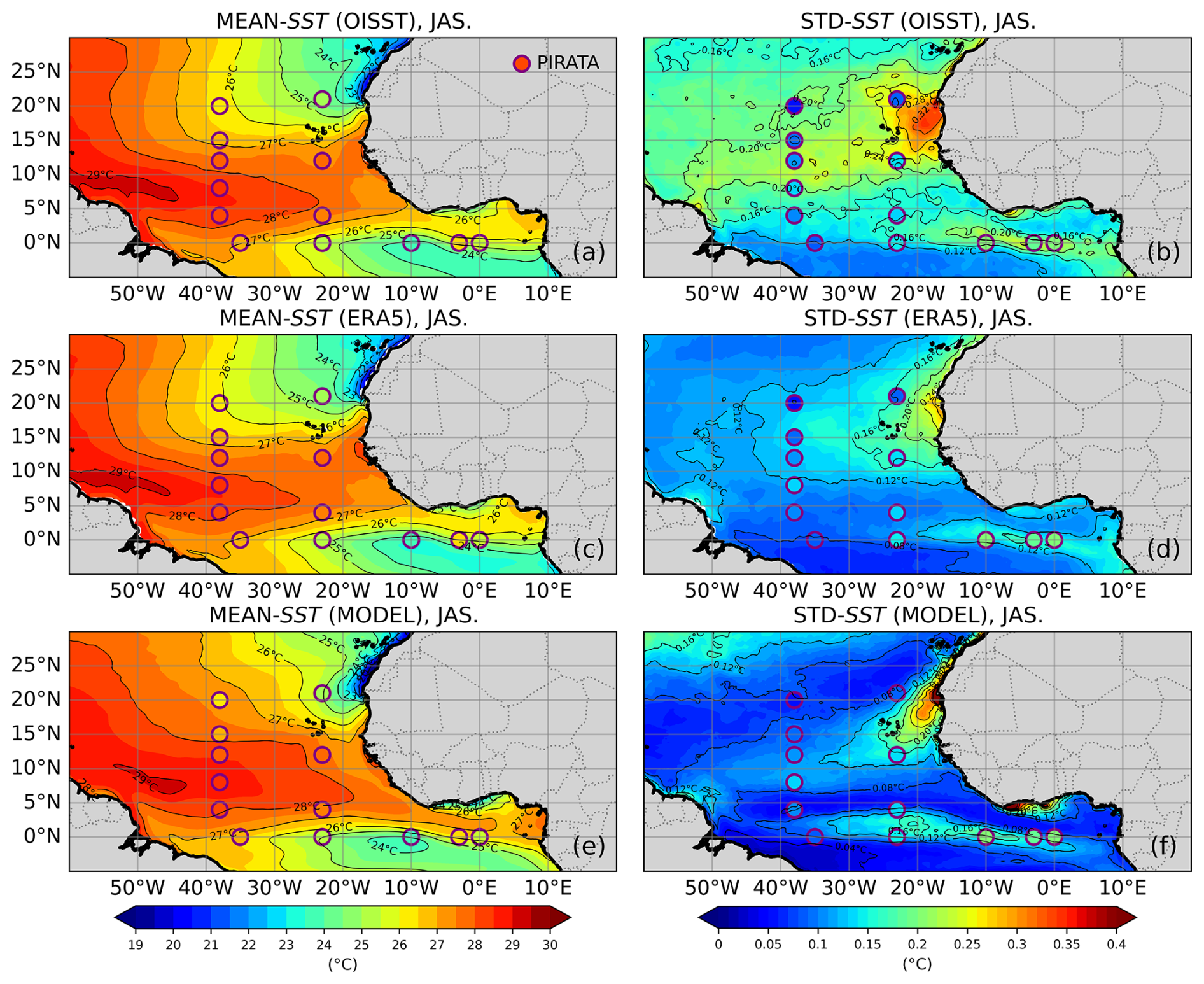
Figure 1 (a, c, e) Mean SST, and (b, d, f) standard deviation of SST anomalies for July–August–September (JAS) over the 2007–2021 period, from (a, b) OISST, (c, d) ERA5, and (e, f) the coupled model. The standard deviation is computed from anomalies band-pass filtered in the 2–10 d range. In each panel, estimates from the PIRATA mooring are indicated by circles.

The standard deviation of SST anomalies filtered in the 2–10 d band reveals substantial amplitude differences among the various products (Fig. 1b, d, and f). OISST exhibits larger synoptic variability than the other datasets, while ERA5 shows comparatively weaker variability at these time scales. Differences in synoptic SST variability among OISST, ERA5, and the coupled model likely arise from a combination of factors, including analysis methodology, spatial smoothing, and effective temporal sampling, as documented in previous intercomparisons of SST products (e.g. Huang et al., 2021a; Reynolds et al., 2007). Previous studies also have shown that ocean surface temperatures can be particularly sensitive to high-frequency atmospheric forcings, such as variations in wind speed, cloud cover and radiative fluxes, particularly at timescales of less than a week (Murray et al., 2000; Donlon et al., 2002).

To assess the realism of synoptic SST variability, we place particular emphasis on comparisons with in situ observations from PIRATA moorings, which provide SST measurements at a depth of approximately 1 m and are consistent with the vertical resolution and daily averaging of the coupled model. This comparison indicates that the coupled model reproduces the amplitude and spatial distribution of SST variability over the 2–10 d band better than ERA5 (Fig. 1d and f).

In particular, the coupled model accurately reproduces two regions of high synoptic variability in SST observed by PIRATA: a zonal band along the northern front of the Atlantic cold tongue, between 0–5° N, and a south-westerly band further north, between 10–20° N. These structures are also present in the other datasets, although their amplitude varies. The coupled model's ability to reproduce these observed configurations confirms its relevance for studying the response of the ocean surface to synoptic atmospheric variability, particularly AEWs, in the tropical Atlantic.

Figure 2 presents the SST climatology (from 2007 to 2021) and the standard deviation of SST anomalies filtered in the 2–10 d band for different datasets at 23° W–11.5° N, corresponding to the location of a PIRATA mooring in a region of high SST variability (Fig. 1f). The seasonal cycle of SST is broadly consistent across the different estimates (Fig. 2a). The model has a warm bias of about 1 °C relative to PIRATA from March to May, while biases during the rest of the year remain smaller than 0.5 °C. However, larger differences are observed in the amplitude of high-frequency variability in SST (Fig. 2b), which is consistent with the spatial patterns identified in Fig. 1b, d, and f. OISST exhibits significantly higher variability over a 2 to 10 d period than the other products, followed by ERA5, which shows intermediate variability and weak seasonal modulation. The coupled model, on the other hand, agrees well with PIRATA observations, reproducing both the amplitude and the seasonal cycle of synoptic SST variability, with a marked maximum during the boreal summer (JAS). This specific comparison supports the use of PIRATA observations as the primary reference for assessing high frequency SST variability and confirms the ability of the coupled model to represent this variability in the region.

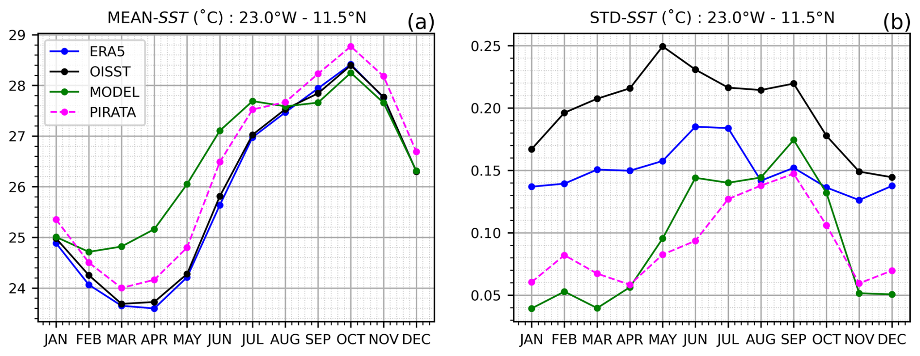
Figure 2 (a) Monthly climatology of SST, and (b) standard deviation of SST anomalies at 23° W–11.5° N over the 2007–2021 period of OISST (black), ERA5 (blue), the coupled model (green), and the 23° W–11.5° N PIRATA mooring (pink). Anomalies are band-pass filtered in the 2–10 d range prior to computing the standard deviation.

3.2 10 m winds

We now assess the ability of the model to reproduce surface wind conditions by comparing 10 m winds from the coupled model with those from ERA5, the ASCAT scatterometer, and in-situ PIRATA measurements. Figure 3 presents the mean 10 m wind (speed and direction) and the standard deviation of band-pass filtered anomalies in the 2–10 d range for the JAS period. On average, the different products show the convergence of the trade winds from the North–East and South–East towards the region of maximum SST (here >27 °C, Fig. 1), which appears to be a response of the winds to the SST anomalies (Sweet et al., 1981; Wallace et al., 1989). This pattern defines the ITCZ, located west of 30° W and around 8° N at this time of year. The ITCZ then tilts northward (between 10–15° N) in the eastern tropical Atlantic, following the SST maximum (Gill, 1980). South of the equator, the southeasterly trade winds cross the equator and are then deflected to the right by the Coriolis force, giving rise to south-westerly winds north of the equator. Laden with moisture, these winds bring the West African monsoon to the continent during the northern summer. These characteristics are very well reproduced by the coupled model, despite a slight positive bias (<0.5 m s⁻¹) compared to ASCAT. ERA5 winds are closer to PIRATA and ASCAT in the vicinity of the ITCZ and along the West African coast, while slightly weaker winds are found over other parts of the basin. Exhibiting a pattern similar to the 2–10 d SST variability (Fig. 1), the 10 m wind variability is pronounced along the West African coast and extends offshore. The largest amplitudes are found off Senegal and Mauritania, where the standard deviation reaches values of up to about 2 m s⁻¹, consistent with the strong synoptic modulation of the low-level flow in this region.

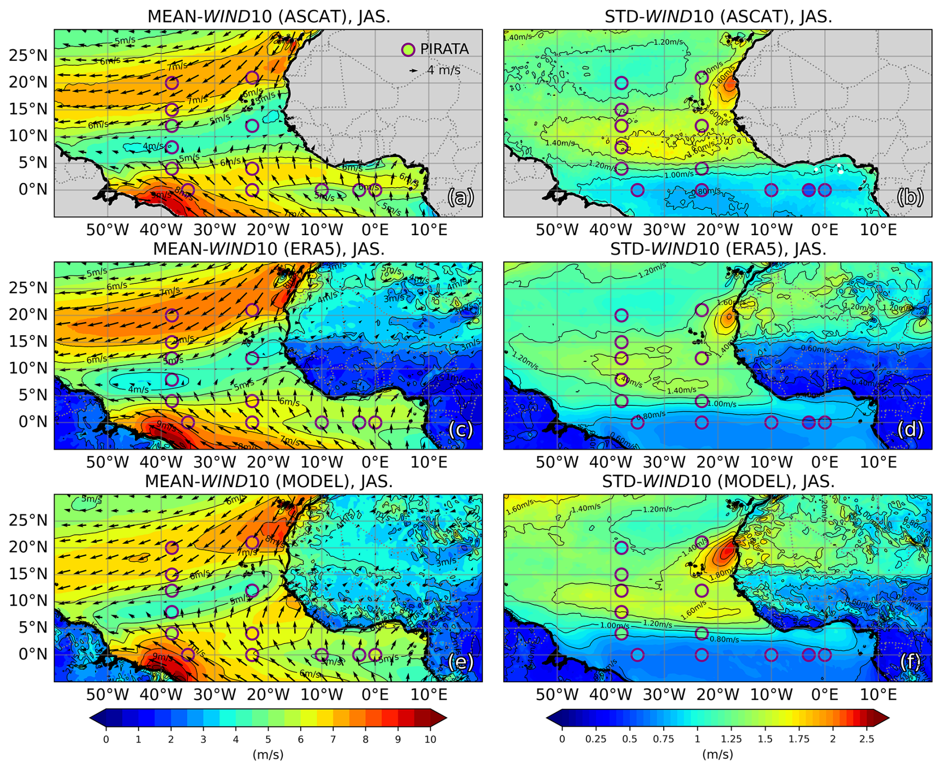
Figure 3 10 m wind speed for the months of July–August–September (a, c, e) and corresponding standard deviation (b, d, f) over the 2007–2021 period for (a, b) ASCAT, (c, d) ERA5 and (e, f) the coupled model. The standard deviation is computed from anomalies filtered in the 2–10 d band. In each panel, PIRATA mooring values are indicated by circles.

The monthly climatology of the 10 m wind and the corresponding standard deviation of anomalies in the 2–10 d frequency band are shown in Fig. 4 for the model, ERA5, ASCAT and the PIRATA mooring at 23° W–11.5° N. A clear seasonal cycle is evident in all datasets, with minimum wind speeds during boreal summer associated with the passage of the ITCZ, and maximum values in winter. The different products exhibit similar seasonal fluctuations, with mean wind speed differences generally smaller than 0.5 m s⁻¹. The 2–10 d variability of the wind at 10 m peaks in summer, consistent with enhanced AEW activity, and shows only minor differences among the datasets, typically below 0.2 m s⁻¹.

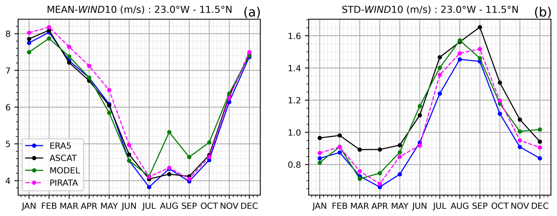
Figure 4 (a) Monthly climatology and (b) monthly standard deviation of the 10 m wind speed at 23° W–11.5° N over the 2007–2021 period for ASCAT (black), ERA5 (blue), the coupled model (green), and the 23° W–11.5° N PIRATA mooring. The standard deviation is computed from anomalies filtered in the 2–10 d band.

3.3 Vertical wind structure

In this region, wind variability on timescales of 2–10 d is largely driven by AEWs. However, this range is quite broad, and it is well known that there are actually two distinct regimes, which we will refer to as southern and northern AEWs, each characterized by different vertical structures, periods, and horizontal distributions (Diedhiou et al., 1998b, 1999; Felice et al., 1990; Viltard et al., 1997). The objective here is to assess whether the model can accurately capture both types of AEWs: those with periods of 3–5 d (hereafter AEWs_3–5 d) and those with periods of 6–9 d (hereafter AEWs_6–9 d).

Figure 5 presents a meridional section of the mean zonal wind (shown as contours) and the standard deviation of the meridional wind anomalies (shown as shading) for the ERA5 reanalysis and the coupled model. Meridional wind anomalies are band-pass filtered in the range of 2–10 d, as well as separately in the 3–5 and 6–9 d bands, and the results are zonally averaged between 25–15° W during the JAS period over 2001–2021. Overall, the coupled model reproduces large-scale vertical structures that are broadly consistent with those represented in ERA5. Although the previous sections show that ERA5 underestimates part of the synoptic variability, particularly near the surface, this comparison remains useful for assessing the consistency of the simulated large-scale circulation patterns. The model produces a stronger wind signal than ERA5, with differences around 1 m s⁻¹ for the mean zonal wind and about 1.25 m s⁻¹ for the standard deviation of the meridional wind. The African Easterly Jet is clearly distinguishable, with its core located near 600 hPa and 15° N, and wind speeds of 13 m s⁻¹ in ERA5 and 11 m s⁻¹ in the coupled model. At the level of the African Easterly Jet, two maxima of meridional wind variability are observed: around 15° N for AEWs_3–5 d and around 25° N for AEWs_6–9 d. A maximum of meridional wind variability at low altitude (around 900 hPa) is also observed between 16–18° N for AEWs_3–5 d. These features are consistent with two AEWs regimes described by Wu et al. (2013). Around 10° N, the West African westerly jet (WAWJ) is visible, with mean winds reaching 3 m s⁻¹ in ERA5 and about 5 m s⁻¹ in the coupled model. It extends from the surface to 800 hPa, and is known to supply moisture from the ocean to the West African rain system (Lamb, 1983; Grist and Nicholson, 2001; Liu et al., 2020). The 3–5 d filtered meridional wind variability highlights transient synoptic disturbances consistent with the typical synoptic variability associated with AEWs. However, interactions between AEWs and the WAWJ cannot be ruled out. AEW-related anomalies can locally and temporarily modulate low-level westerly winds, leading to apparent spatial overlap between the WAWJ region and the AEW signal in surface wind diagnostics. This AEW-WAWJ coupling and its influence on low-level convergence and moisture transport have been addressed in previous studies (e.g. Hsieh and Cook, 2007; Leroux and Hall, 2009). Nevertheless, we interpret Fig. 5e primarily as the surface footprint of AEWs_3–5 d.

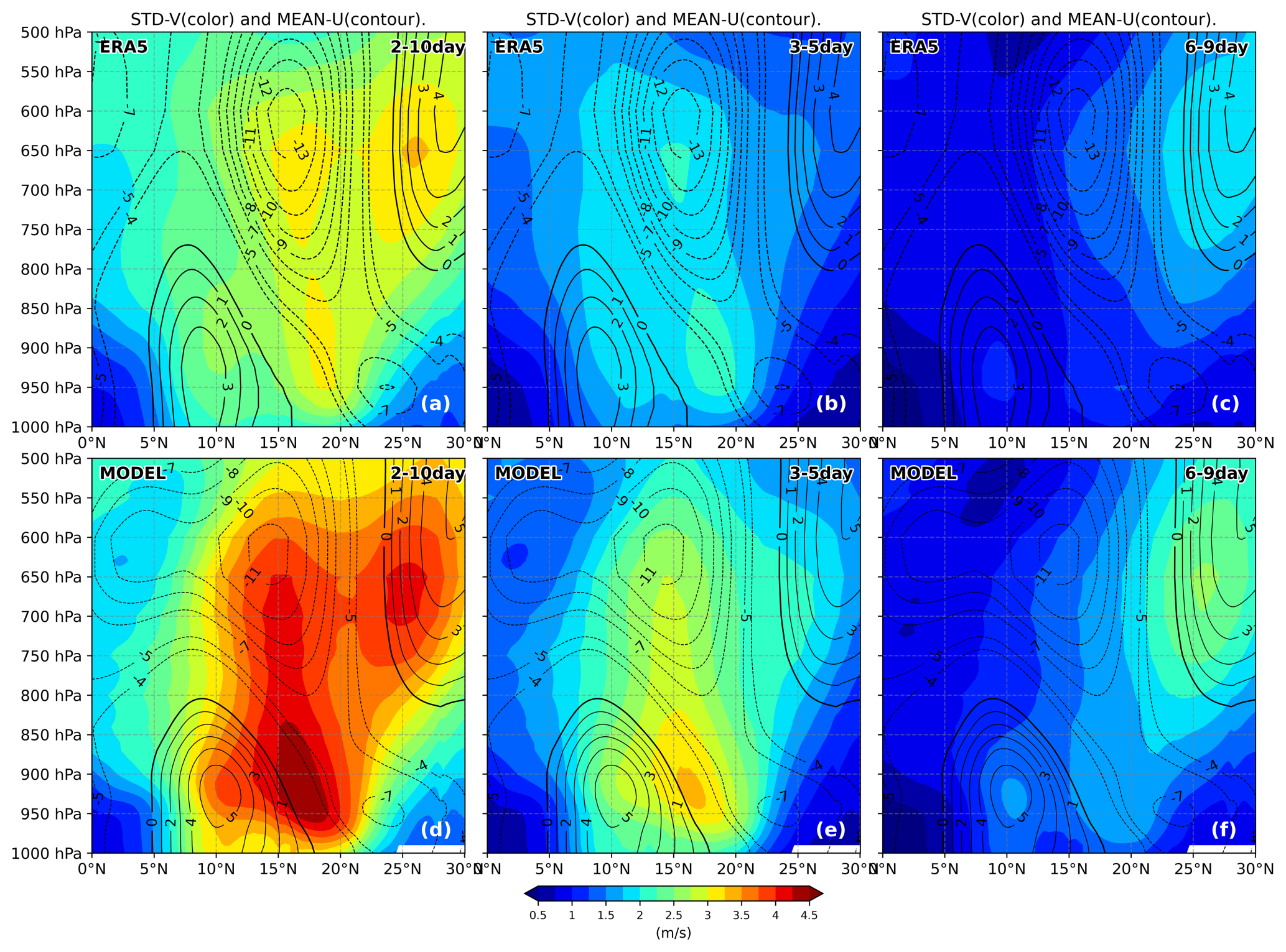
Figure 5 Latitudinal section of the standard deviation of meridional wind anomalies, longitudinally averaged between 25–15° W, during JAS over the 2001–2021 period for (a, b, c) ERA5 and (d, e, f) the coupled model. Anomalies are band-pass filtered in the 2–10 d (a, d), 3–5 d (b, e), and 6–9 d (c, f) ranges. Mean zonal winds are shown as contours to highlight the zonal jets.

Overall, this comparison between the coupled model and atmospheric and oceanic datasets suggests that the model provides a representation of the main characteristics of AEWs and SST variability. It also suggests that the 3–5 d band concentrates most of the surface wind variability, indicating that AEWs_3–5 d are expected to exert the strongest influence on surface processes and SST variability.

4 Ocean surface response to AEWs

4.1 An index representative of AEWs

The colocalization of high wind and SST variability bands near 10° N (Figs. 1 and 3), together with the peak variability observed during JAS, strongly suggests a link between AEWs and the high-frequency variability of SSTs. The influence of AEWs on the ocean surface of the TNA is assessed by projecting the anomalies of relevant physical fields onto an index designed to be representative of AEW activity. In many previous studies, this index has been derived from the characteristic fields at the heart of these disturbances, such as meridional wind, relative vorticity, or outgoing longwave radiation (OLR), and has been applied to atmospheric variables (Diedhiou et al., 2001; Fink and Reiner, 2003; Jiang et al., 2023; Kiladis et al., 2006). Given our focus on the impact of AEWs on SST, and the distinctive surface signature of AEWs (Fig. 5), we have selected a 10 m surface wind index corresponding to the mean meridional wind filtered over the 2–10 d period. The reference point for this index is set at the PIRATA mooring located at 23° W–11.5° N a region of enhanced synoptic variability, sufficiently offshore to avoid coastal effects (Fig. 6). This site is therefore representative of the region of high surface wind variability associated with AEWs. Note that sensitivity tests carried out with other index sites, notably the one located at 17.5° W–15° N proposed by Kiladis et al. (2006), indicate that, despite small variations in local amplitude and statistical significance of the regressions, the large-scale spatial structures and physical interpretation remain similar (not shown).

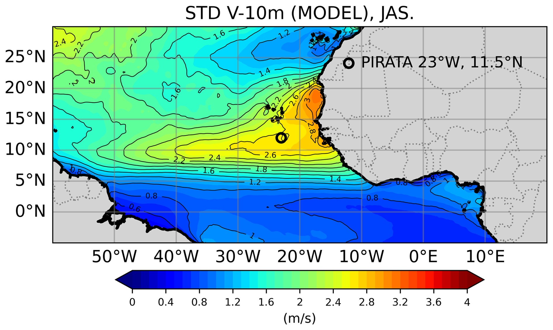
Figure 6 Standard deviation of the 10 m meridional wind anomalies (V-10m), band-pass filtered in the 2–10 d range, during the JAS period from 2001 to 2021 for the coupled model. The location of the PIRATA mooring at 23° W–11.5° N is indicated with a black circle. It lies within the area of maximum variability.

To illustrate the relationship between SST and the 10 m meridional wind at a single location (at 23° W–11.5° N), Fig. 7 shows their evolution during the boreal summer of 2001, together with the corresponding synoptic anomalies. This year was chosen as an illustrative example of the relationship between these two parameters. The 10 m meridional wind alternates between southward (negative) and northward (positive) directions, as the area is located within the ITCZ during this period, resulting in fluctuations ranging from −6–6 m s⁻¹. The high-frequency peaks, although generally offset by about 1–2 d, show a notable degree of correspondence, particularly in July, when strong southward wind bursts are often associated with surface cooling (Fig. 7b). The unfiltered time series (Fig. 7a) highlight the covariability at longer timescales, while the filtered signals (Fig. 7b) isolate the synoptic component. During the boreal summer, much of the variance in the meridional wind is concentrated at the synoptic scale, which explains the relatively small difference between the filtered and unfiltered wind signals. In contrast, SST incorporates atmospheric forcing over longer periods; bandpass filtering therefore eliminates a significant portion of low-frequency variability, resulting in more pronounced differences between filtered and unfiltered SST time series.

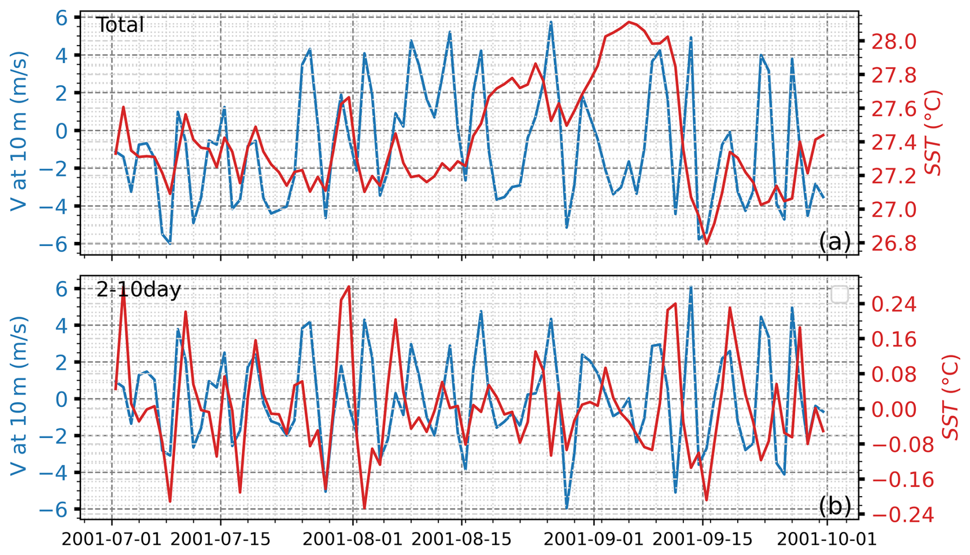
Figure 7 SST (in red) and 10 m meridional wind velocity (in blue) at 23° W–11.5° N during JAS 2001 for the coupled model: (a) non-filtered data, (b) band-pass filtered in the 2–10 d range.

At synoptic timescales, the SST response to wind forcing is intermittent, characterized by variable time lags of about 1–2 d and a non-linear, integrative behavior, so that a strong pointwise linear correspondence is not expected. Nevertheless, several intense southward wind events, particularly in July, are followed by surface cooling, illustrating the influence of synoptic wind variability on SST. Figure 7 is therefore intended as an illustrative example rather than a quantitative assessment of synoptic air-sea coupling, which is addressed in the following sections using regression analyses.

4.2 Signature of AEWs on the SST

To investigate the impact of AEWs on SST, we performed a lagged linear regression analysis using different model variables and the AEWs index, as defined in Sect. 4.1. The following results are subject to a Student's t test, and only the statistically significant local fields (>95 %) are shown.

Figure 8 shows the regression of the meridional wind at different time lags (in d), displaying the evolution of patterns typical of AEWs. Southwest–northeast oriented structures, with a meridional extent of 25–30° (about 3000 km) and a zonal extent of 15°, propagate from east to west. They originate from Central Africa with the lowest amplitude and spread towards West Africa. They reach a maximum amplitude of more than 4 m s⁻¹ over coastal regions at 15–20°, before gradually weakening as they propagate westward into the central basin. This spatial and temporal behavior closely resembles that of structures observed at higher altitudes (e.g. Hsieh and Cook, 2007; Thorncroft et al., 2008; Leroux and Hall, 2009).

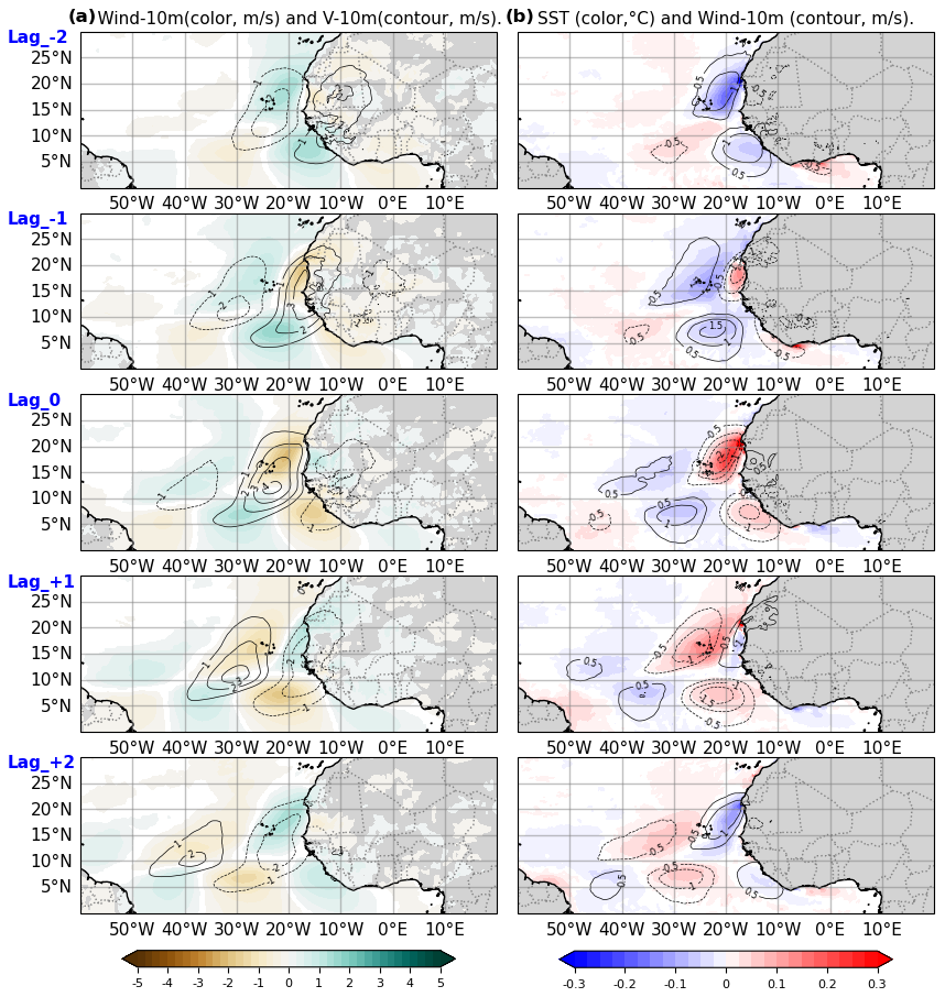
Figure 8 Lagged regression of atmospheric and oceanic variables onto the 2–10 d AEWs index, defined as the 10 m meridional wind anomaly at 23° W–11.5° N (with a positive index corresponding to a northward wind anomaly). Left panels show 10 m wind speed anomalies (color) and 10 m meridional wind anomalies (contours). Right panels show SST anomalies (color) and 10 m wind speed anomalies (contours). Regressions are presented at different time lags (in d) to capture the temporal evolution associated with AEWs passage. The AEWs index time series used here is illustrated in Fig. 7.

As they propagate westward, AEW structures associated with 2–10 d 10 m meridional wind anomalies exert opposite effects on the total surface wind field on either side of the Intertropical Convergence Zone (ITCZ). Specifically, a positive meridional wind anomaly leads to a weakening of the total wind speed north of the ITCZ and a strengthening of the wind south of it (Fig. 8a). The SST anomalies regressed on the AEW index exhibit coherent cooling and warming patterns that propagate westward in phase with AEW-related wind anomalies (Fig. 8b). Stronger surface winds are generally associated with negative SST anomalies, while weaker winds correspond to positive SST anomalies. The mean amplitude of the AEW-related SST response is on the order of ±0.3 °C. More pronounced local anomalies are observed during the most intense events, as identified by the sensitivity tests described in Sect. 2.3, with amplitudes that can exceed ±0.5 °C. AEWs thus play an important role in modulating SST variability in the tropical North Atlantic through surface wind forcing.

5 The ocean mixed layer heat balance

To better characterize the mechanisms through which AEWs modulate SST in the TNA, we analyze the heat budget of the oceanic mixed layer (Jouanno et al., 2011a). This approach is particularly well-suited for isolating and quantifying the physical processes that drive temperature changes in the surface layer, including air-sea heat exchanges, horizontal advection, and vertical diffusion. All terms of the heat budget are computed online in the coupled model. The temperature evolution in the surface layer, for a layer of thickness h, can be expressed as follows:

$$\begin{array}{ll}{\displaystyle }{\partial }_{t}T=& {\displaystyle }-\langle u{\partial }_{x}T{\rangle }_h-\langle v{\partial }_{y}T{\rangle }_h-\langle w{\partial }_{z}T{\rangle }_h+\langle D_t{\rangle }_h\\ {\displaystyle }& {\displaystyle }+{\displaystyle \frac{{\left(K_z{\partial }_{z}T\right)}_{z=-h}}{h}}+{\displaystyle \frac{Q_{\mathrm{s}}\left(\mathrm{1}-F_{-h}\right)+Q_{\text{ns}}}{{\mathit{\rho }}_{\mathrm{0}}{c}_{p}h}}\end{array}$$

Here, T represents temperature; u, v, and w correspond to the zonal, meridional, and vertical currents, respectively; 〈*〉_h, the vertical averaging over the surface layer of thickness h. D_t represents lateral diffusive processes, and K_z is the vertical diffusivity evaluated at the base of the surface layer. The terms Q_s and Q_ns correspond to the net shortwave and non-solar surface heat fluxes, respectively, Q_ns including net longwave radiation as well as sensible and latent heat fluxes. The constant ρ₀ is the reference seawater density, and c_p is the specific heat capacity of seawater. F_−h denotes the fraction of shortwave radiation that penetrates to depth h. In this study, h is set to 5 m to ensure that the integrated trends remain consistent with near-surface ocean conditions.

Overall, the equation expresses temperature evolution as the sum of contributions from horizontal and vertical advection, lateral and vertical diffusion, and atmospheric forcing through Q_s and Q_ns. Terms associated with oceanic processes (advection and diffusion) are grouped under T_OCEAN, while atmospheric terms are separated into non-solar surface fluxes (T_Q_ns) and the shortwave component (T_Q_s).

5.1 Oceanic processes vs. heat fluxes in AEW-induced SST evolution

As with SST, the different terms were time-filtered within the 2–10-day range prior to performing the regressions. Regressions were computed for the JAS period at time lags ranging from two days prior to two days after the AEW index, enabling us to track the evolution of each term during an AEW passage. For comparison, lagged regressions of 10 m wind speed, outgoing longwave radiation (OLR) and mixed layer depth are also superimposed. Note that OLR is used here as an indicator of convective activity associated with AEWs.

Figure 9 shows the regressions of the total temperature tendency and the different heat budget terms on the AEW index. As noted earlier, the impact of AEWs on SST is strongest in coastal regions, where their signature is most pronounced, and gradually weakens as they propagate offshore (Fig. 9a). At zero lag, the regression shows warming around 23° W–11.5° N, corresponding to a northward wind anomaly at the index location and a negative total wind speed anomaly. The evolution of SST associated with AEWs appears to result from multiple processes acting together. All of these processes contribute significantly to temperature changes, with none being negligible, and their effects are not perfectly in phase. Term T_Q_ns (Fig. 9b) exhibits patterns resembling the overall temperature tendency but opposite to the wind anomalies, which can be explained by the fact that increased wind speed enhances latent heat flux (not shown), leading to SST cooling. Although weaker, solar radiation also contributes to the overall trend, which is linked to the modulation of cloud cover (OLR, contours in Fig. 9c). For example, a cooling rate of −0.2 °C d⁻¹ for T_Q_s corresponds to an OLR minimum of −20 W m⁻², and vice versa. Interestingly, these contributions are out of phase with T_Q_ns, with the largest effects occurring north of 10° N, near the ITCZ during JAS.

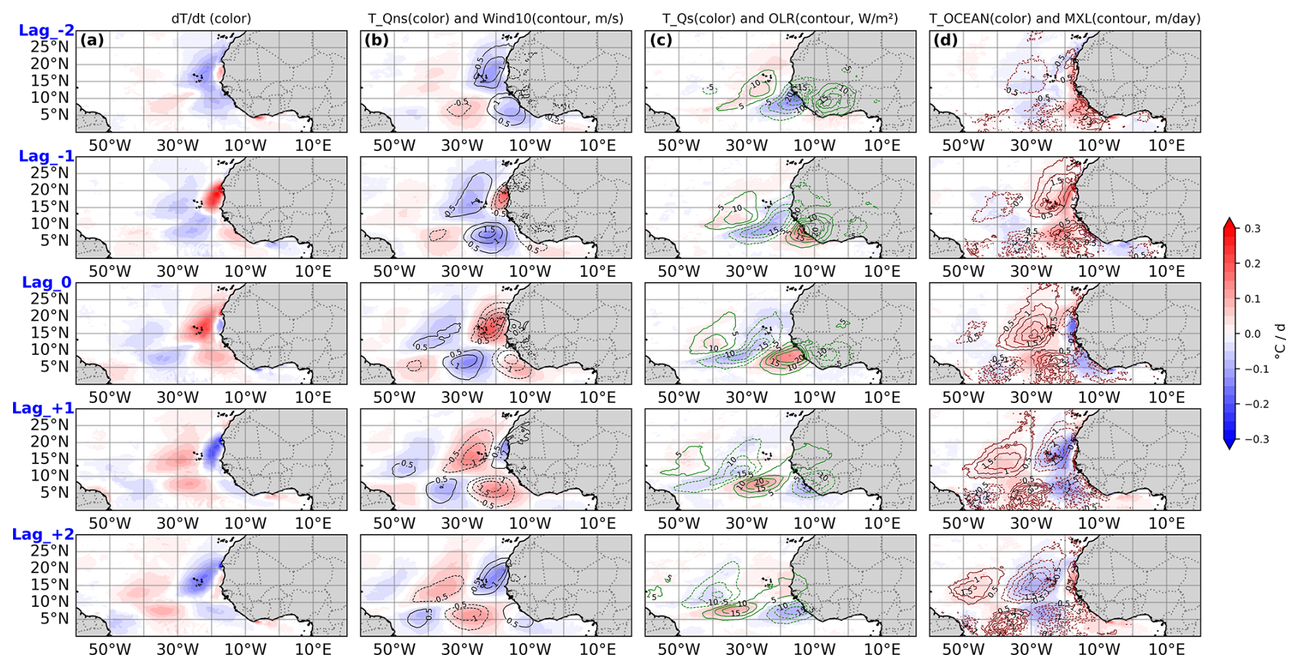
Figure 9 Lagged evolution of anomalies in the upper 5 m ocean heat budget terms, regressed onto the 2–10 d AEWs index. Panels show: (column a) mixed-layer temperature tendency ($\mathrm{d}T/\mathrm{d}t$), (b) contribution from non-solar surface heat fluxes (T_Q_ns, color) with 10 m wind speed anomalies overlaid (contours), (c) contribution from solar radiation (T_Q_s, color) with OLR anomalies (contours), and (d) oceanic processes (T_OCEAN, color) with mixed-layer depth (MXL) anomalies (contours). Regressions are presented at different time lags (in d) to capture the temporal evolution associated with AEWs passage.

The contribution of oceanic processes to SST modulation represents a key part of the ocean's response to AEWs (Fig. 9d). Note that thermal advection is negligible offshore and very weak near some coastal areas. Vertical mixing (vertical diffusion) primarily controls T_OCEAN (not shown). The observed cooling and warming patterns correspond, respectively, to positive (deepening) and negative (shallowing) mixed layer depth anomalies of approximately ±2 m.

The temporal evolution at different lags indicates that the cooling induced by T_OCEAN is associated with increasing wind speeds (Fig. 9b), and that the two signals (wind and T_OCEAN) are in phase quadrature. This indicates that the intensified winds associated with AEWs deepen the mixed layer, entraining cooler subsurface water to the surface and thereby cooling the SST. At zero lag, T_Q_ns cooling rates reach approximately −0.2 °C d⁻¹, while T_OCEAN (mainly vertical mixing, not shown) accounts for up to −0.15 °C d⁻¹, confirming that both mechanisms contribute with comparable magnitudes. This oceanic contribution refers to the T_OCEAN term; the predominance of vertical mixing is inferred from model diagnostics and is not explicitly displayed here. Thus, the SST response to AEWs results from a complex interplay between the effects of local wind speed on air-sea fluxes, the modulation of solar radiation by cloud cover, and the mixed layer deepening during phases of wind fluctuations.

Previous observational studies of the heat budget of the mixed layer, such as Foltz et al. (2003) and Hummels et al. (2014), have focused primarily on seasonal to interannual variability, rather than synoptic timescales. Therefore, to our knowledge, there is currently no direct observational reference documenting the decomposition of temperature trends in the mixed layer at synoptic time scales.

Nevertheless, these studies highlight the important role of vertical mixing in regulating surface temperature variability under the effect of increased wind forcing. In addition, the seasonal heat balance from this model has already been discussed in Gévaudan et al. (2021) and previously in a series of studies (Jouanno et al., 2011a, b), all of which emphasize the important role of vertical mixing in this balance. The synoptic results presented here are therefore consistent with previous seasonal assessments, while extending the analysis to higher frequency variability.

5.2 Dissociating the impact of AEWs in the 3–5 and 6–9 d bands

As discussed previously, AEWs occur over two distinct time scales, typically corresponding to the 3–5 and 6–9 d bands, which have different meridional distributions. Consequently, the regression results presented earlier may be biased toward the more dominant wave band. To determine whether similar processes occur for both wave types, we perform regression analyses of $\mathrm{d}T/\mathrm{d}t$ and its contributing terms using indices filtered separately for each band (Fig. 10). The results confirm that AEWs in the 3–5 d band have a significantly greater impact on SST compared to those in the 6–9 d band. This is consistent with the surface signature of AEWs_3–5 d between 5–25° N, as opposed to the higher-altitude and more northerly AEWs_6–9 d structures (Fig. 5).

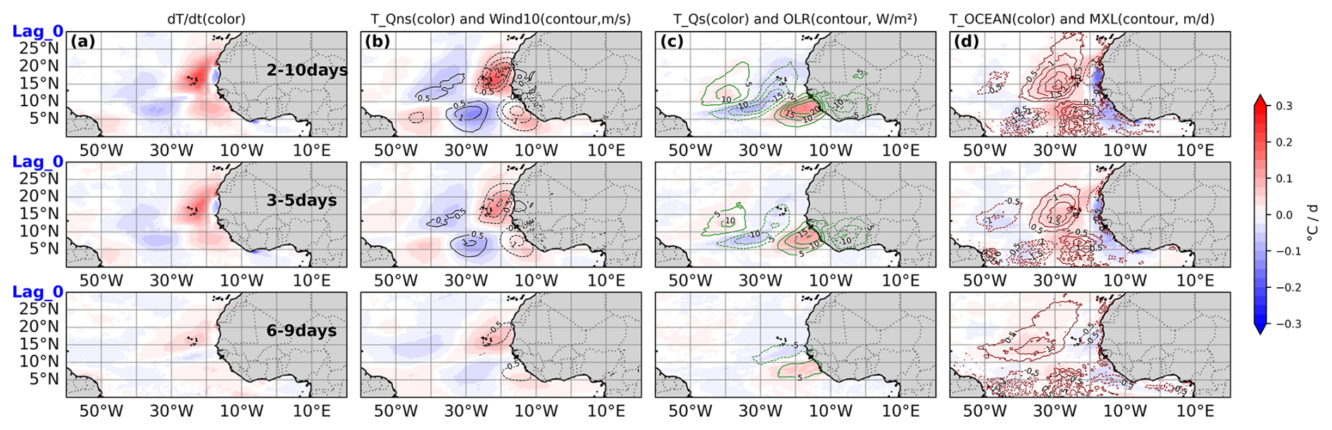
Figure 10 Same as Fig. 9, but shown at lag 0 only. Panels present anomalies in the surface layer temperature tendency ($\mathrm{d}T/\mathrm{d}t$) and its contributing terms for the 2–10 d (top panels), 3–5 d (middle panels), and 6–9 d bands (bottom panels).

As a result, 3–5 d waves more effectively force air-sea heat fluxes and mixed layer processes, leaving a clear imprint on SST. Although this behavior is physically expected given the respective wind structures, its quantitative expression in terms of SST response and contributions to the heat balance is not trivial a priori, due to the integrative and non-linear nature of the ocean mixed layer response. The comparison between the two frequency bands therefore clarifies the dynamic mechanisms by which AEWs influence the ocean surface. For both types of AEWs, the results indicate that the SST response arises from a combination of air-sea fluxes and vertical mixing, which contribute in comparable proportions, although the overall amplitude of the response is significantly weaker for the 6–9 d band.

6 Conclusions

A 21-year regional coupled simulation over the tropical Atlantic is used to investigate the influence of African Easterly Waves on SST in the TNA and to quantitatively assess the underlying processes. Although small biases in SST and wind are present, comparisons with reference satellite observations and atmospheric reanalysis datasets demonstrate that the simulation provides a robust framework and a solid tool for studying ocean–atmosphere interactions in the tropical Atlantic. The characteristics of AEWs, represented by westward-propagating meridional wind anomalies between 5–25° N, with a typical zonal wavelength of about 15°, are well captured by the simulation and show good agreement with observations and reanalysis datasets. In addition, the temporal separation into 3–5- and 6–9 d variability reveals distinct branches characterized by their latitude and vertical structure, in agreement with the literature.

This study highlights for the first time a robust and consistent AEW-related imprint on SST in the tropical Atlantic, with anomalies of approximately ±0.3 °C on average, increasing to approximately ±0.5 °C for stronger events. The combined effect of latent heat fluxes, shortwave radiation, and vertical mixing underscores the critical role of AEWs in shaping mixed-layer dynamics.

The signature of AEWs on SST is identified by regressing SST anomalies and temperature tendency terms onto filtered wind anomalies used as a representative AEW index onto SST fields, revealing a significant and consistent AEW-related imprint. A similar projection applied to the temperature tendency terms of the heat budget shows that AEW-related SST anomalies result from a combination of non-solar heat flux fluctuations (mainly latent) driven by surface winds, shortwave radiation variations linked to cloud cover changes, and modulation of ocean mixing associated with mixed-layer variability. The results also highlight a stronger SST response between 5–20° N from 3–5 d AEWs compared to 6–9 d AEWs, consistent with their more pronounced surface signal south of 20–25° N. While such methodologies have been applied to atmospheric fields, to our knowledge, this is the first time that this type of identification has been demonstrated for oceanic fields.

This quantitative assessment of the impact of African Easterly Waves (AEWs) on dynamic and thermodynamic heat fluxes is useful when compared to previous studies. Several studies have shown that the role of atmospheric wind and latent heat fluxes dominates variability from intraseasonal to interdecadal timescales (Foltz et al., 2003), while the role of mixing has mainly been identified as being enhancing in the upper thermocline within 2° N–2° S (Jouanno et al., 2011a) relative to off-equatorial regions (Hummels et al., 2014). However, turbulence remains the most challenging component to quantify and assess, and high-frequency phenomena can also contribute to local mixing outside the equatorial region (Foltz et al., 2020; Hummels et al., 2020). Although this mechanism is not explicitly diagnosed here, the mixing component may be partly consistent with the influence of near-inertial motions generated by AEW-related wind forcing, which have been shown to enhance upper-ocean mixing in previous studies over extensive regions of the eastern TNA (D'Asaro, 1985; Plueddemann and Farrar, 2006; Hummels et al., 2020). Further investigation is therefore required to quantify the role of near-inertial activity in the mixing contribution.

This raises questions about our methodology, which relies on regressing SST and heat-budget terms onto a wind-based AEW index. While this approach primarily captures synchronous responses, it may overlook effects that occur out of phase. Tests applying time lags from −2 to +2 d did not significantly change the results. This indicates that, unlike the more immediate effects of solar radiation and latent heat fluxes linked to cloud cover and wind fluctuations, the influence of near-inertial waves generated by AEW-related wind bursts and potentially propagating over several days may be underestimated. This could be addressed through additional numerical experiments, such as masking AEWs by nudging winds toward climatology, to better isolate oceanic processes and their influence on interannual timescales.

Beyond advancing process understanding, the findings of this paper are relevant for improving the representation of synoptic variability in coupled models, reducing persistent SST biases, and ultimately enhancing tropical cyclone prediction and seasonal climate forecasts.