Tide of the Time: Global tidal characteristics observed from in-situ measurements

Tide gauges have been critical sources for sea level research, enabling the development of tidal theory and an understanding of local variations that occur across the global oceans. Tides play important roles in a variety of oceanographic and geodetic applications, and characterizing their spatial variability is valuable for applications ranging from fishing to flood risk management. This manuscript presents the coastal characteristics of ocean tides based on 3591 high-frequency tide gauge observations from the recently updated Global Extreme Sea Level Analysis (GESLA) database. These characteristics range from tidal datums such as Mean High Water (MHW) and the Great Diurnal Range to metrics like the Age of the Tide, Form Factors, updated amplitude trend estimates, and new insights into the regional duration of high tides. Our analysis finds that 125 out of 237 long-time series show statistically significant trends in one or more constituents, from −1.47 to +1.80 mm yr⁻¹, while the duration of the high-water stand during spring tides is shown to vary from 1 to 14 h, for an inundation depth of 20 cm. It is anticipated that the results presented will be useful not only to tidal experts but also to a wide range of cross-disciplinary researchers and local communities, aiding their understanding of a vital component of the global Earth system.

1 Introduction

Tides are a persistent and dominant force shaping the coastal zone, shelf seas, and open ocean. They modulate storm surges and waves (Horsburgh and Wilson, 2007), influencing extreme sea levels, flooding, and erosion (Pugh and Woodworth, 2014), constrain navigation and port access (Akan et al., 2017), and govern vertical ecological zonation in intertidal environments (Stumpf and Haines, 1998). In the open ocean, tidal dissipation affects large-scale circulation and vertical mixing (Munk, 1966; Wunsch and Ferrari, 2004; Green et al., 2009). Across shelf seas, tides drive sediment dynamics (Simpson and Sharples, 2012), underpin tidal energy resources (Robins et al., 2015) and generate coherent turbulence (Smith et al., 1999; Talke et al., 2013), enhancing mixing and air–sea gas exchange (Talke et al., 2013; Zappa et al., 2007), with consequences for carbon dioxide uptake (Thomas et al., 2004) and hypoxia (Talke et al., 2009). Recent studies have shown that multi-year to decadal tidal cycles modulate the frequency of both extreme flood return levels and high-tide flooding (Enríquez et al., 2022; Thompson et al., 2021). In estuaries, interactions among tides, mixing, and river discharge regulate salinity intrusion (Jay, 1991; Geyer and MacCready, 2014), sediment transport, and system morphology, shaping mass, momentum, and energy budgets across the river–estuary–shelf continuum (Jay, 1991; Burchard et al., 2018). Tides also shape river plumes (Horner-Devine et al., 2009) and shelf sea fronts, influencing productivity and fisheries (Simpson and Hunter, 1974). Tidal datums underpin many national boundaries and historical geodetic systems (Shalowitz, 1964). Consequently, tides have significant scientific and practical implications.

Tides have been measured since the 17th century, and tide predictions based on the phases of the Moon and empirical knowledge were made much earlier. Cartwright (1999) discusses early understanding of the nature of ocean tides dating back to ancient civilizations, roughly 2000 BC, while Woodworth (2023) discusses the transformation in tidal science thanks to Newton. Systematic tide-gauge measurements have been collected for more than three centuries, providing one of the longest instrumental records in geosciences. Early tide gauges, installed in major European ports in the 17th and 18th centuries, used simple float or staff mechanisms to record water levels relative to fixed benchmarks. By the late 19th century, standardized stilling-well gauges enabled continuous, high-precision tidal observations, forming the foundation of national networks. The transition to automated digital systems in the late 20th century, which are based on pressure, acoustic, or radar technologies, expanded spatial coverage and improved temporal resolution, supporting modern sea-level research, operational forecasting, and coastal hazard assessment. Concepts such as “the high-water mark” and “ordinary high water” held legal significance but were often nebulous in definition, sometimes leading to disputes over property rights. More scientific measurement and analysis approaches were developed by Whewell (1830s) and William Thomson (1872), in particular, the method of harmonic analysis (more on this later). The increasing scientific rigour led to the introduction of concepts such as mean sea level, mean tidal range, and mean high water, which are rigorously defined and provide first-order statistics on how the ocean interacts with land, and how this varies regionally and globally.

The past 75 years has produced many variations on, and alternatives to, conventional harmonic analysis and tidal prediction, including the response method (Munk and Cartwright, 1966), developments on traditional harmonic analysis programs (Godin, 1972; Foreman, 1977; Pawlowicz et al., 2002; Leffler and Jay, 2009; Codiga, 2011), non-stationary analysis approaches (Jay and Flinchem, 1997; Matte et al., 2013; Pan et al., 2018; Lobo et al., 2024; Monahan et al., 2025), inclusion of derivative constraints (Doodson, 1951; Foreman and Henry, 1979), and other statistical and data processing innovations (e.g. Gan et al., 2021; Su and Jiang, 2023). Moreover, the advent of the digital age and the increasing commitment of many countries to open data have led to the increasing size and data coverage of international tide databases, including that of the World Ocean Circulation Experiment (WOCE) project in the 1990s, the University of Hawaii Sea Level Centre (UHSLC), and, more recently, the community-led Global Extreme Sea Level Analysis (GESLA) database (Woodworth et al., 2017; Haigh et al., 2022). Currently, the GESLA-4 database contains around 130 000 station years of data, spanning 6474 sites (the total unique data is approximately 20 %–30 % less, as many gauge data sets are duplicated). Despite these efforts, available data does not cover all parts of the global coastlines due to either a lack of public data sources or a lack of tide gauges.

This manuscript is intended to provide a synthesis of tidal characteristics from updated in-situ tide-gauge observations, by revisiting established tidal datums with new insights into tidal behaviour. By providing these insights, we aim to offer a coherent reference for tidal dynamics that demonstrates their importance along the coast. This synthesis is intended to support a wide variety of cross-disciplinary applications for both local and scientific communities. The up-to-date synthesis of the best available data and knowledge additionally supports both future modelling and analysis and to help identify knowledge and data gaps.

2 Data

The GESLA project was established to expand global access to hourly and higher-frequency sea-level records, assembling diverse datasets from a range of sources into a common, quality-controlled format to support research on extreme sea levels. The first release, GESLA-1 in 2009, included 21 197 years of data from 675 records and was used in studies of global sea-level extremes (e.g. Menéndez and Woodworth, 2010; Hunter et al., 2017; Marcos et al., 2015) and in the IPCC Fifth Assessment Report. To improve coverage and incorporate new observations, GESLA-2 was compiled in 2015–2016 (Woodworth et al., 2017), expanding the dataset to 39 151 years from 1355 records. GESLA-2 supported extensive research on extreme sea levels, tidal and nontidal interactions, flooding hazards, tidal variability, and model validation, and has contributed to the IPCC Special Report on the Ocean and the Cryosphere and the Sixth Assessment Report.

The third version, GESLA-3, released in 2021 (Haigh et al., 2022), represented a major upgrade: it nearly quadrupled the number of records and doubled the total observation years. GESLA-3 comprised 91 021 years of data from 5119 tide-gauge sites drawn from over 30 global data providers. GESLA-3 refined data processing, added additional metadata, applied uniform format standards, and adhered to FAIR data practices, making it more robust for future research. The most recent and fourth version, GESLA-4, released in 2025 (Haigh et al., 2022, updated), is a compilation of hourly and higher-frequency measurements from 45 agencies across 119 countries, totaling 127 623 station years of data from 6474 sites. The oldest records date back to the 19th and early 20th centuries, with the oldest gauge dating back to 1 January 1800 in Gorinchem, the Netherlands. However, the majority of records date back to the last 20–50 years.

3 Tidal analysis

Tide gauges have been a remarkable source of data for studying ocean tides. The standard technique for determining the astronomical tidal component of a tide gauge record is known as the harmonic method. This technique originated in the work of William Thomson (Lord Kelvin) and George Darwin in the 19th century, building on the insights of Pierre-Simon, Marquis de Laplace. It replaced the earlier non-harmonic methods, which were particularly computationally intensive for their time. Subsequent developments have made the harmonic method the most common technique used by present-day tidal researchers, although alternative approaches, such as various forms of the response method, have been used in some applications. A history of how these methods originated can be found in Cartwright (1999).

The harmonic method parametrises the tide as the sum of N harmonic terms as follows:

$$\begin{array}{}\text{(1)}& {\displaystyle }{\displaystyle }\text{Tide}=Z_{\mathrm{0}}+\sum _{i=\mathrm{1}}^N{f}_i{H}_i\cos \left({\mathit{\omega }}_{i}t+V_i+u_i-G_i\right),\end{array}$$

which is a function of time t. The H_i and G_i are the amplitude and phase lag, respectively, for a particular constituent i with angular frequency ω_i. The term V_i is the equilibrium argument at the origin of time, which thereby provides a connection to the relevant astronomical motions (e.g. Doodson, 1921). The “nodal corrections” f_i, u_i adjust a constituent's amplitude and phase for modulations induced by the 18.6-year motion of the Moon's node (and for some terms the 8.8-year motion of the Moon's argument of perigee); in principle these modulations could be handled directly by a more complete harmonic expansion involving a larger N (e.g. Foreman and Neufeld, 1991), but in practice this is rarely done and the f_i, u_i adjustments that stabilize the system by implicitly modelling the correlation between constituents (a form of regularization) are standard. Z₀ refers to the mean sea level. For more details, see Doodson and Warburg (1941), Parker (2007), Pugh and Woodworth (2014), Egbert and Ray (2017). Permitted values of angular frequency are combinations of six fundamental frequencies associated with the orbits of the Moon and Sun (Doodson, 1921). In practice, only the terms with the largest amplitudes in the “tidal potential” (the gravitational forcing that drives the tides) tend to result in the largest amplitudes in the real ocean. A few dozen terms are usually sufficient for parameterizing the tide in a one-year record to good accuracy; the default standard for NOAA tide prediction is N=37 (Parker, 2007). In nonlinear regimes, many more terms may be required (for example, NOAA uses 120 constituents at Anchorage, Alaska). Most analysts tend to use a set of N terms that work best for their region.

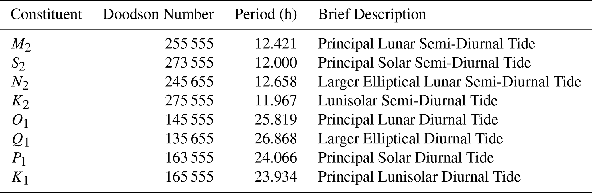
For historical reasons, each major term has a “name” which originated in the 19th-century work of Kelvin and Darwin. The largest term at most locations is M₂, being the principal semidiurnal component due to the Moon. Its period is half a lunar day. Similarly, S₂ is the principal semidiurnal component due to the Sun, with a period of half a solar day. The tide also has diurnal components; the largest at most locations are K₁ and O₁. The former stems from a combination of both lunar and solar forcings, while the latter is purely lunar. Terms with names such as M₄ and M₆ result primarily from frictional and other nonlinear hydrodynamical effects at coastal margins and shallow estuaries (Andersen et al., 2006), and have periods of $\mathrm{1}/\mathrm{4}$ and $\mathrm{1}/\mathrm{6}$ of a lunar day (the subscript denotes the approximate number of times a constituent repeats per day). Table 1 presents eight of the major components and their associated periods, while Parker (2007) provides a more comprehensive list.

Table 1 Major tidal constituents and their characteristics.

The dominant tidal constituents commonly found in most parts of the ocean are readily identified by power spectral density analysis, as in Fig. 1, which shows high power at similar frequencies in two gauges even though they are in different ocean regions. Particularly evident are peaks in the diurnal (daily) and semi-diurnal (twice daily) bands, corresponding to the primary astronomical forcings. The amplitudes and phase lags of each of these terms at a particular location are calculated by fits to a tide gauge record, generally using least-squares techniques. Once calculated, the set of H_i and G_i values (referred to as “harmonic constants”) can be used to calculate the tide far into the future (or past). In fact, the estimated harmonic constants depend strongly on the reference data used to estimate them, which can induce apparent variations in H_i and G_i when shifting the reference epochs. They may exhibit, seasonal and interannual variability (Devlin et al., 2014), primarily driven by meteorological factors, and can even change over decades or more, as discussed in Sect. 6. Variability can also be caused by inaccuracies in measured water levels or time (e.g. Zaron and Jay, 2014). Nevertheless, one can usually analyse a tide gauge record to arrive at a “best set” of such constants.

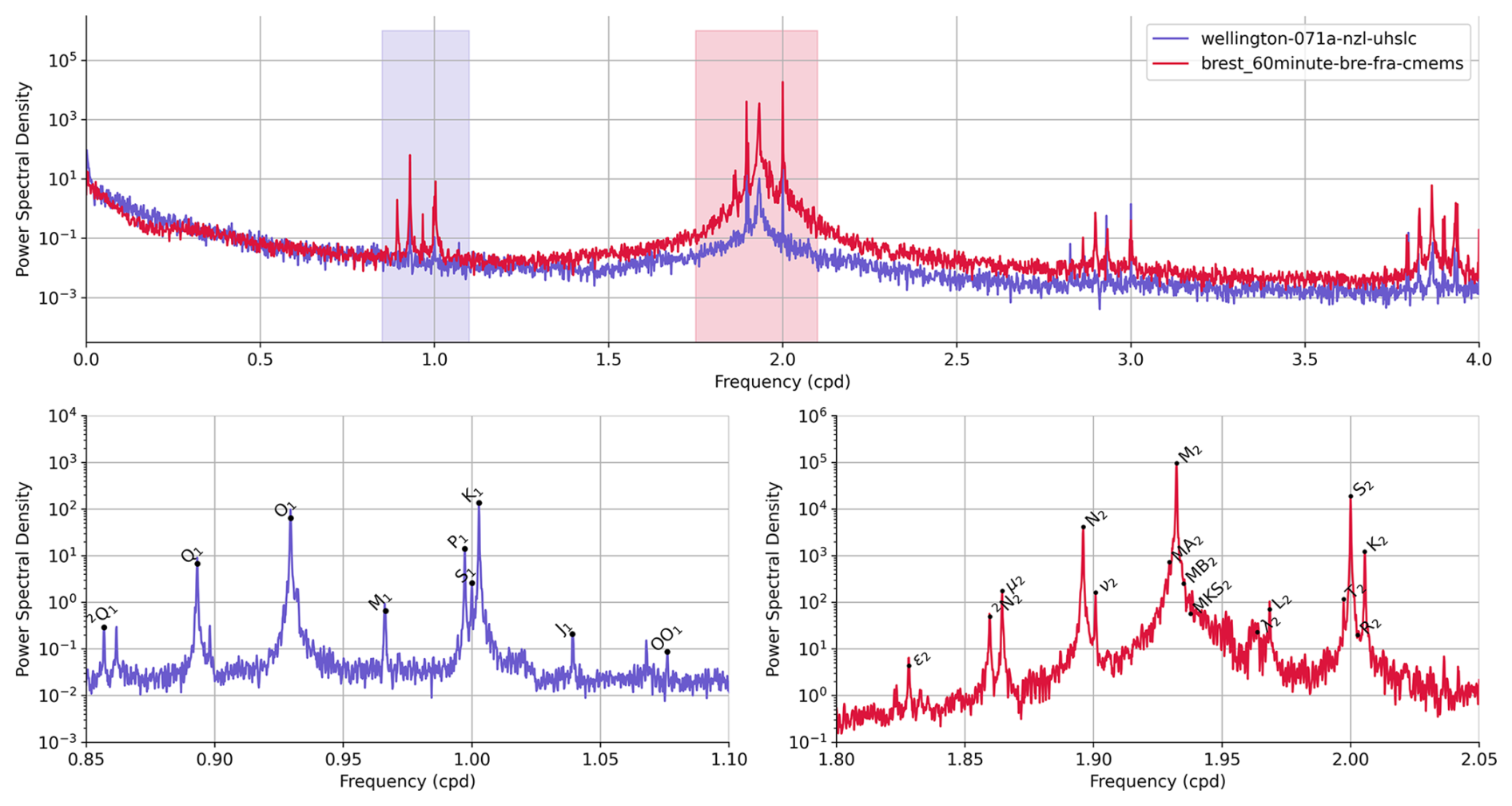
Figure 1 Spectral analysis of the Wellington (blue) and the Brest (red) tide gauge, as well as zoom-ins to the semi-diurnal and diurnal band of the Brest gauge, highlighting several tidal constituents.

In this context, the harmonic analysis approach was employed to create a database of 50 tidal constituents, known as TICON-4 (Hart-Davis et al., 2025), based on the GESLA-4 database, which is used to generate the results presented throughout the paper. For more information on TICON-4, see Hart-Davis et al. (2025). In this study, we reduced the TICON-4 to 3591 by removing data from rivers and lakes, as well as from regions such as the Baltic Sea and the Black Sea, which are characterized by negligible tides. The extensive GESLA-4 dataset contains several gauges along the Gulf of Mexico coast, which we observe are located within swamplands. For the analysis within this manuscript, these gauges are removed as they do not have significant tidal signals (amplitudes typically smaller than 2 mm), and they bias the mean statistics. Additionally, the estimation of tides is susceptible to timing changes or errors, which are attempted to be resolved within TICON-4 using an iterative procedure (see the user manual of Hart-Davis et al., 2025). Despite this effort, some errors may still occur and influence the findings (Pan et al., 2025; Thompson et al., 2025). To combat this, we utilize the uncertainty information from TICON-4 to remove any gauge that contains errors that exceed the signals from our analysis.

It is important to note that several additional methods exist for tidal analysis. These include the response method (Munk and Cartwright, 1966; Monahan et al., 2025), the wavelet-based approach (Lobo et al., 2024), and the species concordance method (George and Simon, 1984), as well as methods that modify the harmonic analysis approach (Matte et al., 2013; Pan et al., 2023). Within this manuscript, we rely solely on the harmonic method, due to it being the most widely used method for tidal analysis and the method employed in the TICON-4 dataset. However, a future study could assess the differences in tidal analysis approaches and the impacts this could have on tidal statistics or tidal predictions.

The reconstruction of the tidal sea surface heights can be performed by evaluating Eq. (1) at arbitrary past or future epochs. In general, prediction methods implicitly employ more harmonics than can be derived from measurements, especially if the original time series is short. Standard methods of “tidal inference” have been developed for this (Parker, 2007). A standard method of tidal inference is nodal corrections, i.e. f_i, u_i, introduced earlier. Another approach is given by the matrix formalism shown in Appendix A. This technique has been previously employed to compute tides in space geodesy (Kvas et al., 2019), and it encodes the long periodic variations of tidal phases and amplitudes of the so-called pivot tides (here: N=50), by implicitly estimating a larger number M of minor partial waves from the tide-generating potential. As with inference methods, the elements of the matrix are derived by assuming that the tide admittance varies only weakly with tidal frequency and is quasi-constant for tidal constituents (linear admittance). Here, we consider all minor waves to a threshold of 0.001 m² s⁻² from the HW95 tide-generating potential, which amounts to 148 spectral lines (Hartmann and Wenzel, 1994, 1995, see Appendix A).

Both tide-gauge measurements and tidal predictions can be used to characterize tidal regimes through various statistical properties and a number of standard “tidal datums,” such as mean low water (MLW) (a summary of these datums are presented in Table B1 and visualized in Fig. B1). Although most tidal datums are traditionally based on water-level measurements, usually over a complete nodal cycle, we here use tidal predictions based on the TICON-4 constants (as outlined in Appendix A). This allows us to include many tide gauges with a duration of less than 19 years, but always at least one year (a TICON-4 restriction to ensure the highest-accuracy constituents). It also removes from the computed datums any possible non-tidal oceanographic effects, although in most cases these are not expected to be noticeable. Our tidal predictions extend over 200 years, from 1900 to 2100, sampled every 15 min. For each time series, we identify tidal highs and lows as local extreme values. From the series of extreme values, we compute the overall highest and lowest astronomical tide (HAT and LAT), and the tidal range as the difference between successive highs and lows.

Additionally, the computed values include the mean high water (MHW) and mean higher high water (MHHW), which is the average of the higher high water of each two consecutive maxima (equivalently for low waters: MLW and MLLW). Together, these tide levels provide a comprehensive description of the tidal regime and the intertidal zone, which allows drawing connections to local biological and geological processes, e.g. the habitability for specific species or the boundary conditions of sedimentation processes. For example, knowledge of local tide levels is important for interpreting Sea Level Index Points related to a specific intertidal zone in sea level reconstruction (e.g. Hijma et al., 2015).

4 Tidal constituents

It is not uncommon to see tidal investigations focus on only the eight “major” constituents. The importance of these eight tides (listed in Table 1) is highlighted in Fig. 2, where the median variance explained for each constituent globally is presented. The principal semi-diurnal lunar tide, M₂, unsurprisingly explains the largest percentage of variance, 62.0 %, and is shown to be the constituent with the largest tidal amplitude for tide gauges throughout the global oceans.

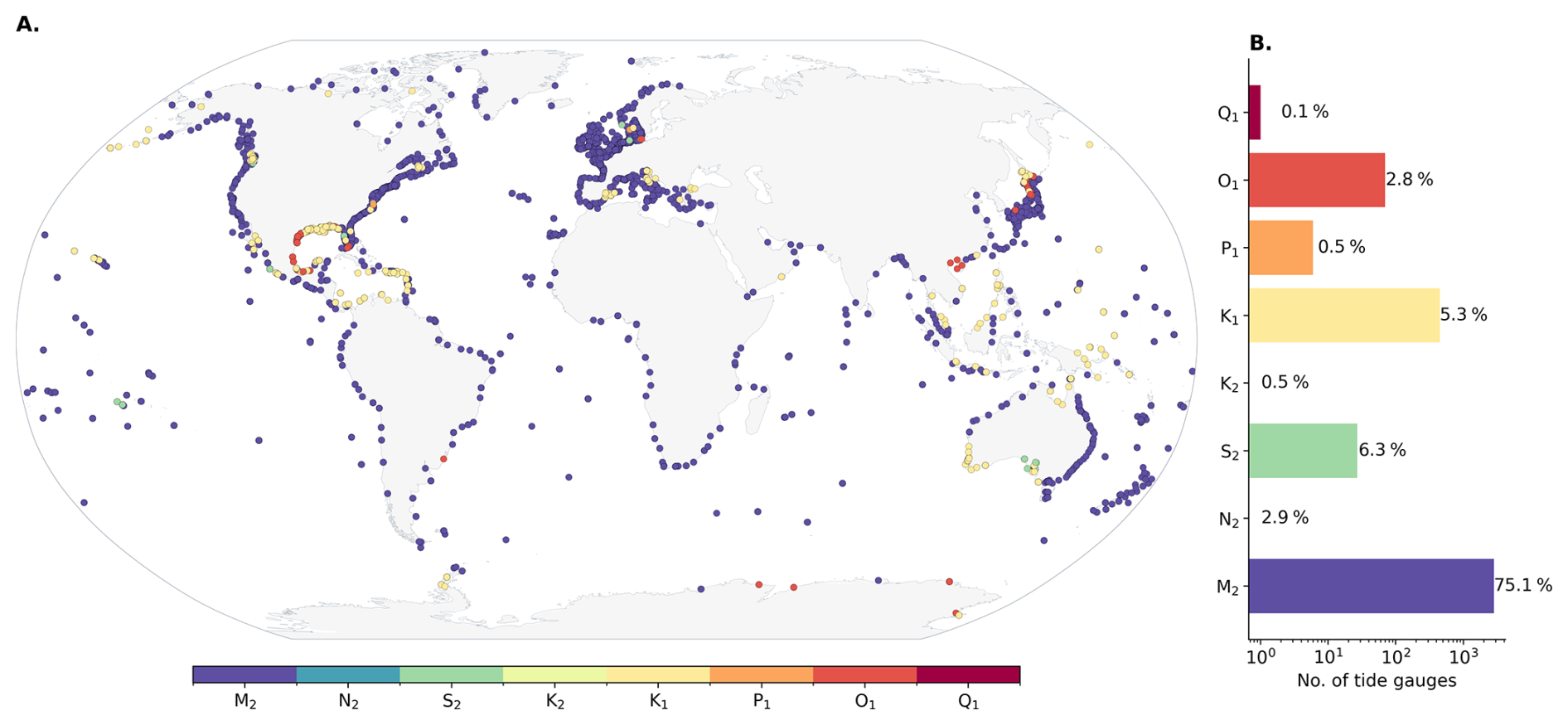
Figure 2 (A) The largest major constituent for each tide gauge as well as (B) the number of tide gauges where a constituent is the largest. The percentage numbers are the median explained percentage variance of each constituent.

The eight major tidal constituents (Table 1) explain a total of 74.8 % and are found to have larger tidal amplitudes compared to the remaining tidal constituents for 88.1 % of tide gauges globally. Despite the significant influence of the semi-diurnal components, there are known regions, such as the Gulf of Mexico and the southwest coast of Australia, that are dominated by the diurnal constituents. While our analysis focuses on coastal tide gauges, the derivation of tidal constituents can be influenced by nontidal processes, such as river dynamics (this is expanded upon in Sect. 7). To knowledgeable tidal enthusiasts, this is noted with the P1 tide being the largest. In our analysis, we determine 5 tide gauges where this occurs, but in all occasions these gauges are within lagoons or in protected coastlines, such as ports, where no significant tidal signal is observed, with tidal amplitudes not exceeding 5 mm in these locations.

Despite the importance of major tides, the remaining tidal constituents – the “minor” tides – are still of considerable importance (Egbert and Ray, 2017). Based on TICON-4, we calculate that the amplitude of at least one minor tide exceeds that of the major tides in 15.0 % of coastal tide gauges; when evaluating gauges within rivers only, this increases to 50.5 %. In Fig. 3C, the largest minor tide from each tide gauge is presented, with the cumulative counts presented in Fig. 3A. The ν₂, M₄, and μ₂ constituents are revealed as the most dominant minor tides, which are observable throughout the global coasts. The ν₂ and μ₂ being of such importance is particularly crucial, as studies by Hart-Davis et al. (2021) have discussed the challenges of estimating these constituents from satellite altimetry within global ocean tide models, due to signal-to-noise issues and perturbations from nonlinear effects. In many global models, these two constituents are accounted for in tidal prediction by inferring them via admittance approaches. The MA₂ and MB₂ are particularly important in higher latitudes along the Canadian coast (Fig. 3C), as these constituents are manifestations of the seasonal variability of the M₂ tide, which is caused by various factors, including sea ice cover (Ray, 2022).

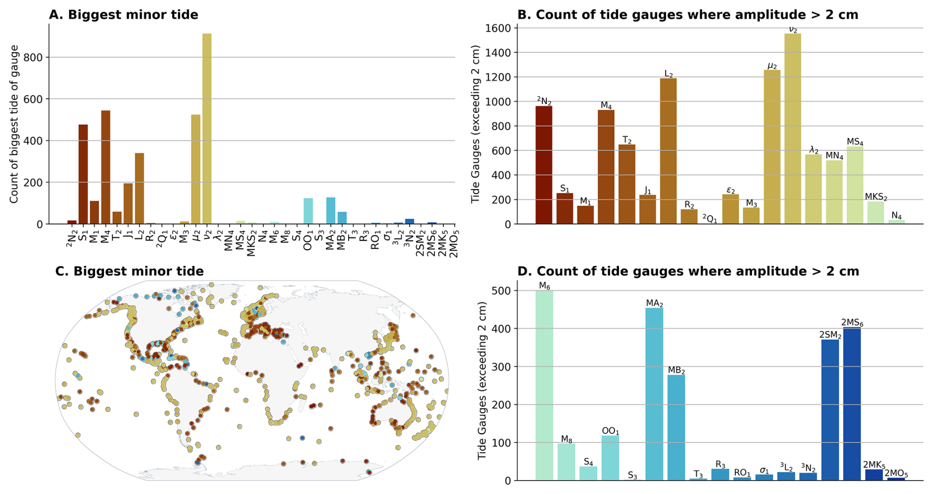
Figure 3 The largest minor tide and the number of gauges when a constituent exceeds a 2 cm amplitude.

Shallow water constituents form as a result of nonlinear interactions with major tidal constituents, causing asymmetry in the tidal waves and leading to their formation. The physical mechanisms underlying the appearance of nonlinear constituents are reviewed in detail by Le Provost (1991). The M₄ constituent, a fundamental harmonic of the major M₂, is known to reach large amplitudes in some shelf waters, exceeding 50 cm in the Bristol Channel, and it is identified in Fig. 3A as one of the largest minor constituents. Several shallow-water tides, such as the 2SM₂ and 2MS₆, exhibit amplitudes exceeding 2 cm at many tide gauges, highlighting not only the complexity of tides in local regions but also the value of tide gauges in resolving these tides. From a data-derived tide modelling standpoint, resolving these shallow water tides is rather challenging, with state-of-the-art models deriving only a handful of the largest of these constituents (Lyard et al., 2021).

Some recent efforts in the modelling community have begun work on the long-neglected third-degree tidal constituents (Woodworth, 2019; Ray, 2020; Sulzbach et al., 2022). These tides result from a small asymmetry in the tidal potential, and in the diurnal and semidiurnal bands they can be detected most readily only in long (>8-year) time series. Although observed amplitudes are typically relatively low, usually in the single millimeter range and rarely exceeding 1 cm, in TICON-4, we identify that the ³N₂ and ³L₂ constituents exceed 2 cm amplitudes at 20 tide gauges. The terdiurnal M₃ can be larger, exceeding 10 cm on some localized shelf resonances (Huthnance, 1980). Overall, a large number of the 33 constituents have amplitudes exceeding 2 cm across the numerous tide gauges (Fig. 3B and D), with 23 of these constituents exceeding this threshold for more than 100 tide gauges. This further emphasises the importance of minor tidal constituents and of accounting for their contributions to tidal predictions, both directly from observations and within global tide models.

The long-period tides, with periods ranging from 1 week to 18.6 years, are not included in our analysis in Fig. 3, allowing emphasis to be placed on the daily and sub-daily bands; however, their exclusion does not diminish their importance. These constituents (Sa, Ssa, Mm, Mf, Mt, etc.) are produced by various motions of the Sun and Moon that, in essence, modulate the forcing for the Earth's permanent tide. They are generally only a few cm or smaller. At many coastal gauges, MSf is inflated by nonlinear effects (its frequency equals the difference between S₂ and M₂ frequencies). The Sa constituent, however, is a “meteorological tide,” driven by seasonal climatic effects associated primarily with the sun's annually varying declination. Owing to this strong forcing, the observed Sa is usually the largest of the long-period constituents (on average, about 7.6 cm); see Fig. 6C below. The semiannual Ssa is also primarily meteorological, but it also has a significant gravitationally driven part (e.g. Ray et al., 2021). See also Ponte and Schindelegger (2024) for a more extensive discussion of these two long-period constituents as seen at coastal tide gauges.

5 Tidal characteristics

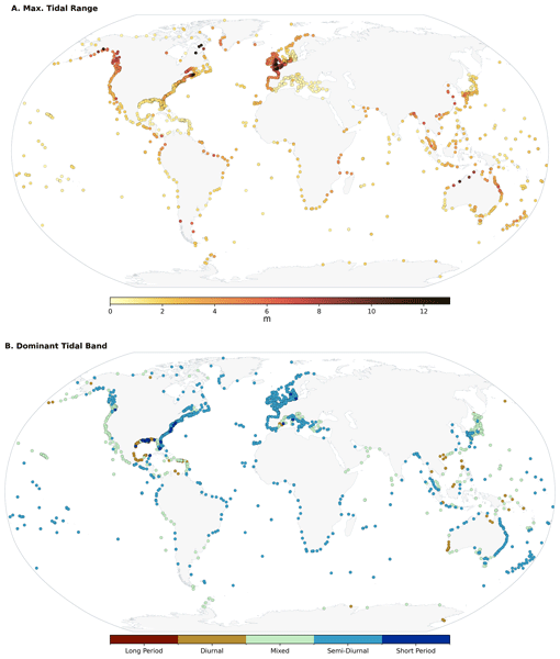
Along large stretches of the world's coastlines, tides play a crucial role in coastal flooding events, either amplifying or dampening the effects of high-water events commonly caused by storm surges. The contribution of tides to coastal flooding largely depends on the tidal amplitude, or tidal range, which is defined as the height difference between successive low and high tides. Figure 4A displays the maximum tidal range. Tidal ranges differ greatly across global coastlines, from only a few cm in semi-enclosed seas such as the Mediterranean, the Baltic, and the Caribbean, to exceeding 10 m in macrotidal areas such as the Bay of Fundy, the English and Bristol Channels, the Patagonian Shelf, and northern Australia.

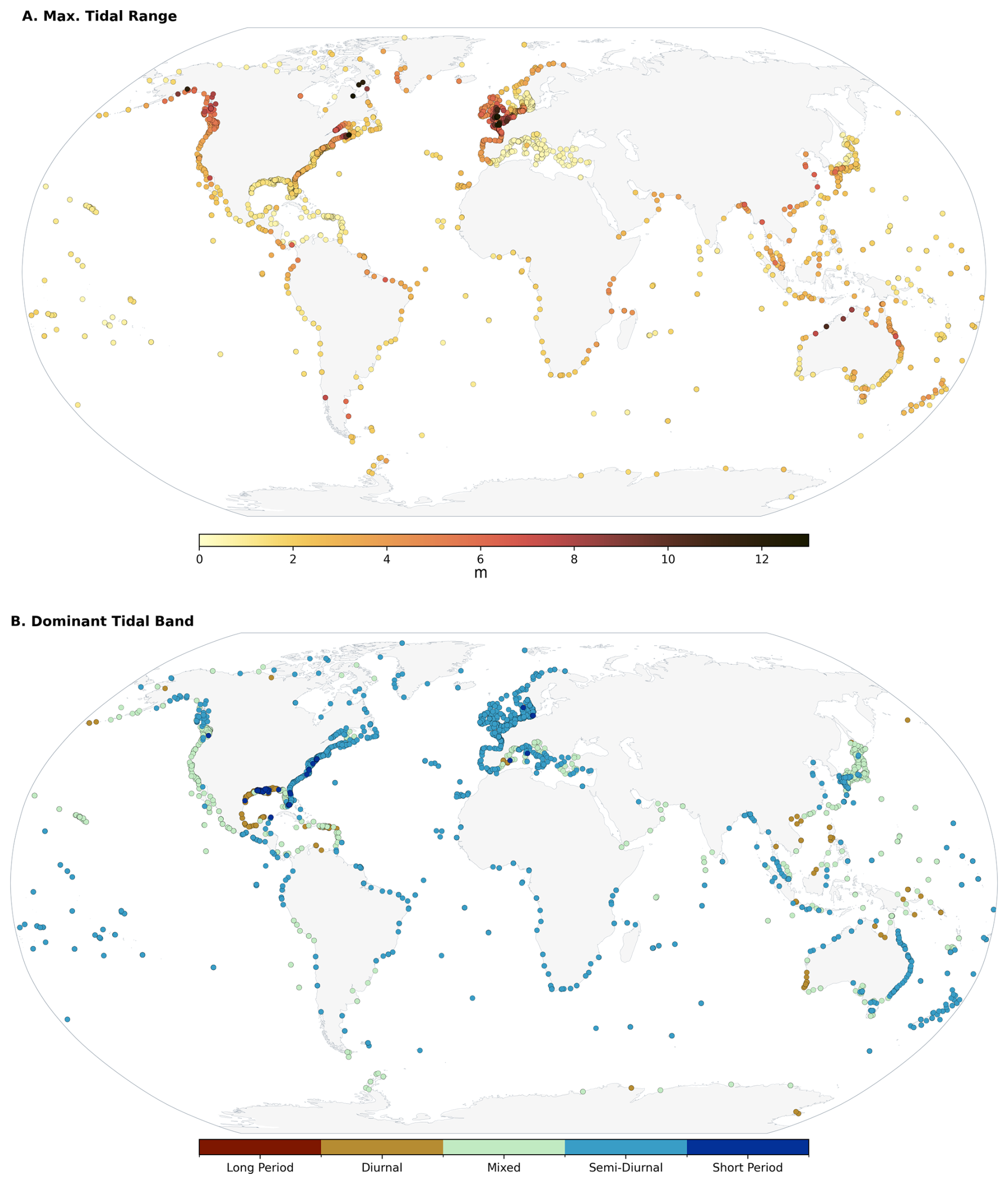
Figure 4 The tidal range and dominant tidal band for each tide gauge in GESLA-4. In Fig. B2, examples are shown of tide gauges in each tidal band.

Naturally, the global distribution of HAT, MHW, and MHHW (Fig. 5) is quite comparable to the maximum tidal range. A slightly altered pattern is displayed in Fig. 5D, which shows MHHW-MHW, i.e. the average height difference of two consecutive high waters. Higher values are obtained for mixed tidal regimes with considerable amplitudes. Tide gauges are strongly influenced by diurnal and semi-diurnal tidal processes due to the forcing produced by the Moon and the Sun. However, depending on the tide gauge's position and location and the region's oceanographic characteristics, the relative contributions of semidiurnal and diurnal tides vary. Typically, tidal frequencies are categorized into different tidal regimes: long-period tides (lasting longer than 24 h), diurnal tides, mixed tides, semi-diurnal tides, and short-period tides (with periods shorter than 12 h). Several measures provide insights into which frequency band is most energetic. For example, the sum of tidal constituent amplitudes within each respective tidal band provides an approximation for which band contributes most to high and low water (Fig. 4B). When the sum of the diurnal and semidiurnal amplitudes is within 50 % of each other, water levels follow a “mixed” tidal regime with a pronounced inequality in the roughly twice-daily high and low tides.

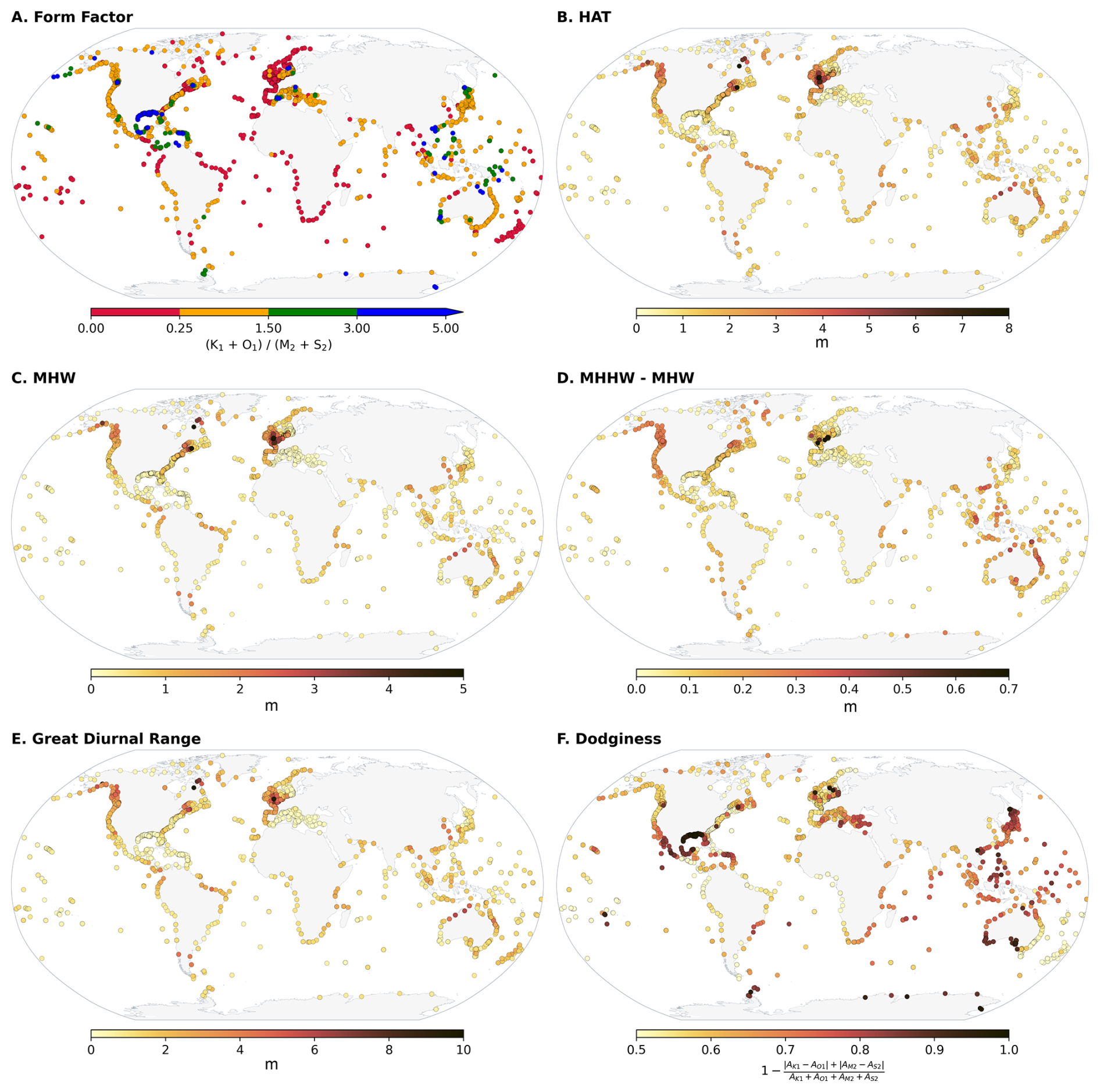
Figure 5 Form Factor, Highest Astronomical Tide (HAT), Mean High Water (MHW), Mean Higher High Water (MHHW), Great Diurnal Range, and Dodginess derived from each tide gauge.

An additional measure that describes the relative contributions of diurnal and semidiurnal forcing is the tidal Form Factor (Fig. 5A). The Form Factor (FF) is the ratio of the two major diurnal constituents (O₁+K₁) to the two largest semidiurnal constituents (M₂+S₂). For FF values lower than 0.25, tides are considered semi-diurnally dominant; for values between 0.25–1.5, tides are considered mixed semi-diurnal; for values between 1.5–3, tides are mixed diurnal; and for values exceeding 3, tides are considered diurnally dominant.

Complementary to FF, we next introduce a “dodginess” parameter that describes the extent to which the apparent amplitude of the local tide varies over a lunar cycle. A significant reduction in this apparent amplitude can occur if the dominant partial tides (frequencies f₁ and f₂) of the respective tidal regime have nearly equal magnitudes. In this case, a tidal beat is created, with the beat frequency $(f_{\mathrm{2}}-f_{\mathrm{1}})/\mathrm{2}$ modulating the amplitude. Often, the constituents at play are M₂ and S₂, as in the case of Port Adelaide situated in the Gulf Saint Vincent in South Australia, which is famous for its “dodgy” tidal regime that tends to completely decay on a fortnightly period (e.g. De Ruyter, 2025). Since a “dodgy” behavior is also possible in diurnal regimes, dominated by K₁ and O₁ (e.g. New Orleans), or mixed tidal regimes (e.g. the South coast of Borneo), we define the parameter “dodginess” as:

$$\begin{array}{}\text{(2)}& {\displaystyle }{\displaystyle }\text{Dodginess}=\mathrm{1}-{\displaystyle \frac{|H_{K_{\mathrm{1}}}-H_{O_{\mathrm{1}}}|+|H_{M_{\mathrm{2}}}-H_{S_{\mathrm{2}}}|}{H_{K_{\mathrm{1}}}+H_{O_{\mathrm{1}}}+H_{M_{\mathrm{2}}}+H_{S_{\mathrm{2}}}}}\end{array}$$

Thus, a value of 1 quantifies a very dodgy tidal regime, while 0 signifies non-dodgy tides. While the parameter does not perfectly capture all possible conditions that produce dodgy tides, it provides a robust metric for estimating the abundance of tidal beating in the world's oceans, which is clearly dominated by the four utilised tides (Fig. 2). Extended dodgy tidal regimes are indicated, e.g. for the Antarctic Coast, the Gulf of Mexico, South Australia, the Gulf of California and the adjacent Mexican West Coast, and parts of the Indonesian Archipelago (Fig. 5F and B3). Further, local resonances cause concentrated dodgy tides, e.g. in the Gulf of Carpentaria and the Gulf of Gabes in Tunisia. The latter represents a curious exception to the generally microtidal Mediterranean Sea with a tidal range of up to 2 m (Sammari et al., 2006). The vast majority of stations are dominated by tidal frequencies within the semi-diurnal range, with a geographical pattern similar to that of the largest major constituents, as shown in Fig. 2 above. Despite this, there are regions driven by diurnal constituents, particularly the Gulf of Mexico and the southwestern coast of Australia. Long-period tidal constituents are typically smaller than those of the higher frequency constituents. In regions such as the Baltic Sea or Black Sea (which are excluded from our analysis), where the tidal range is considered negligible, these long-period constituents are often the dominant signal.

In the remainder of this section, we present a global analysis of several further statistics that help understand tidal dynamics, providing insights useful for a variety of biogeophysical studies, ranging from compound flooding mitigation to ecosystem functioning. In Fig. 6A and B, the age of tide and the age of diurnal tide are presented. The age of the tide is an old, but still scientifically useful, term for the lag between the new or full Moon and the maximum spring tidal ranges. It arises from the ocean tide being unable to respond instantly to the tidal potential forcing but having to adapt to other forces, for example, friction and to large-scale resonances of ocean basins, that contribute to its dynamics (Garrett and Munk, 1971; Webb, 1973) (The large-scale character of this parameter can be seen better in Fig. B3).

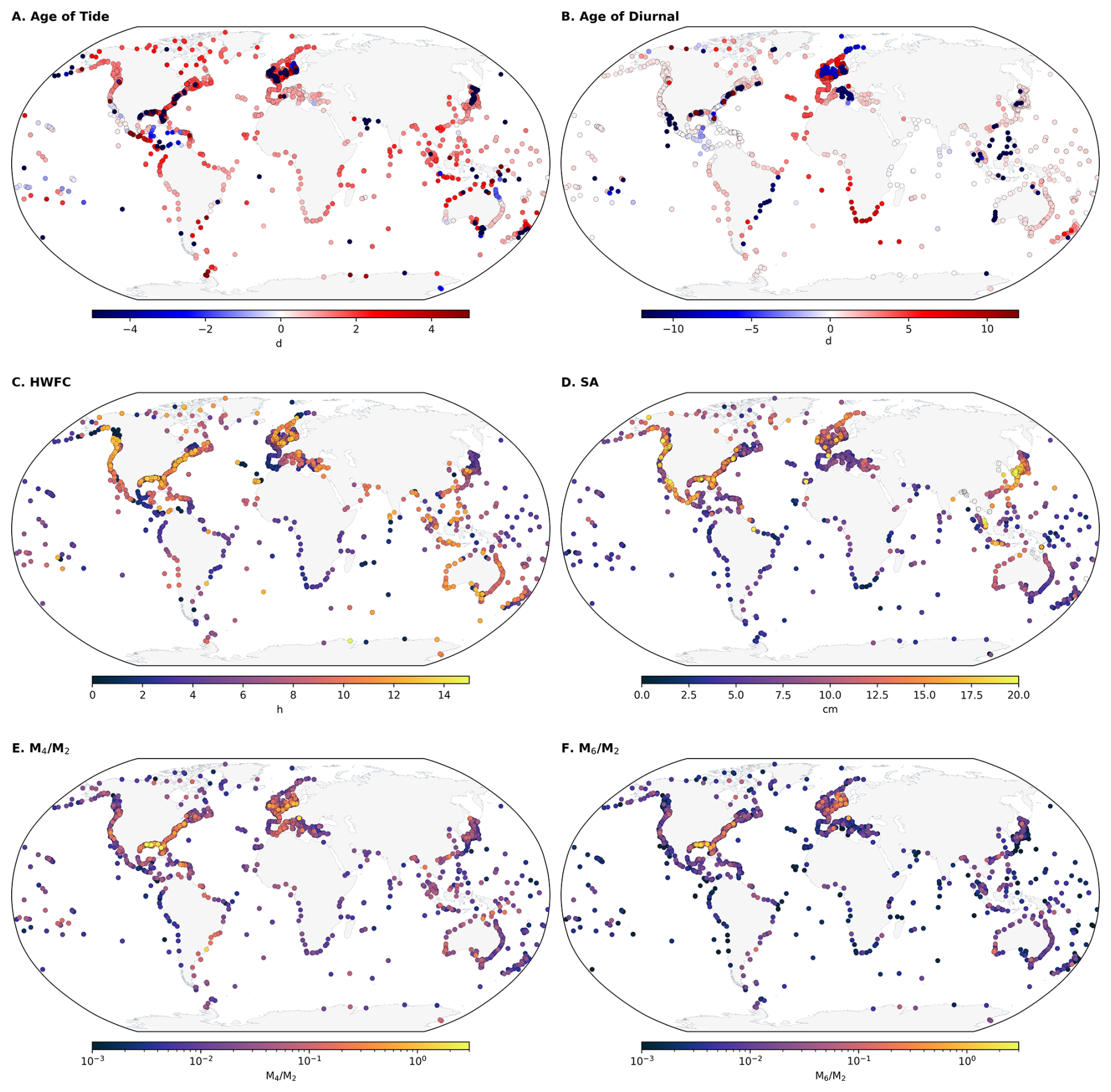
Figure 6 Age of Tide, Age of Diurnal tide, HWFC, Solar Annual (Sa) constituent, ratio of $M_{\mathrm{4}}/M_{\mathrm{2}}$, and ratio of $M_{\mathrm{6}}/M_{\mathrm{2}}$. A selection of these results is shown for the FES2022 model in Fig. B3.

The age of the semidiurnal tide at any one location is given by:

$$\begin{array}{}\text{(3)}& {\displaystyle }{\displaystyle }\text{Age of semidiurnal tide}=(G_{S_{\mathrm{2}}}-G_{M_{\mathrm{2}}})/(S_{S_{\mathrm{2}}}-S_{M_{\mathrm{2}}})\end{array}$$

where $G_{S_{\mathrm{2}}}$ and $G_{M_{\mathrm{2}}}$ are the Greenwich phase lags of the S₂ and M₂ constituents and $S_{S_{\mathrm{2}}}$ and $S_{M_{\mathrm{2}}}$ are their speeds. Alternatively, local phase lags, usually denoted by the Greek symbol κ, can be used for this calculation, where $\mathit{\kappa }=G+nL$, n being the species (2 in this case) and L the longitude east of Greenwich. $S_{S_{\mathrm{2}}}$ and $S_{M_{\mathrm{2}}}$ denote the speeds in degrees per solar hour of S₂ and M₂ (30 and 28.984° h⁻¹, respectively). This lag (or age) typically has a positive value of several hours, though it varies by location. For example, it has a value of 18 h in New York and 8 h in San Francisco, but it is actually negative in Honolulu (Pugh and Woodworth, 2014). Liverpool's value is approximately 2 d, which is about the global average. In other words, the solar tides on average lag behind the solar tidal forces by a larger amount than the lunar tides lag behind the lunar forces (Doodson and Warburg, 1941). Previous maps of the age of the semidiurnal tide can be found in El-Sabh et al. (1987), Gil and De Toro (2005). Overall, the average positive age of the tide is a consequence of tidal dissipation. More concretely, one would expect larger tidal amplitudes only after the occurrence of a full Moon, since the full Moon is the cause for large tidal forces and, thus, amplitudes. Therefore, at a first glance, regions with a negative age of the tide, e.g. the Coral Sea (Webb, 1973), seem to contradict causality. However, this can be a consequence of the oceans' resonant nature, in which tidal energy is permanently redistributed, leading to a spatially and temporally localized concentration by interference that leaves causality untouched.

Similarly, an age for the diurnal tide can be computed, which is the interval in hours between the maximum declination of the Moon and the time of high water of the following (diurnal) spring tide (Doodson and Warburg, 1941). In harmonic terms, it can be represented by:

$$\begin{array}{}\text{(4)}& {\displaystyle }{\displaystyle }\text{Age of diurnal tide}={\displaystyle \frac{G_{K_{\mathrm{1}}}-G_{O_{\mathrm{1}}}}{S_{K_{\mathrm{1}}}-S_{O_{\mathrm{1}}}}}.\end{array}$$

where $G_{K_{\mathrm{1}}}$ and $G_{O_{\mathrm{1}}}$ are the Greenwich phase lags of the K₁ and O₁ constituents and $S_{K_{\mathrm{1}}}$ and $S_{O_{\mathrm{1}}}$ are their speeds. Previous maps of the world coastline for this quantity have been presented by El-Sabh and Murty (1989); values vary considerably spatially, with the largest (approximately 57 h) in the Atlantic and the smallest (approximately 4 h) in the Indian Ocean.

The lunitidal interval is the time between the transit of the Moon and the next high water at a particular location. It varies over the spring-neap cycle, with its average over the cycle called the Mean High Water Interval (MHWI) or “corrected establishment”. Its value near the time of full and new Moon is called High Water Full and Change (HWFC) or “vulgar establishment”. HWFC is larger than MHWI by about half an hour if the age of the tide is about 2 d, as is the case for many locations around the world. These quantities seem somewhat archaic nowadays, but in the days of sailing ships, captains would have been intimately familiar with HWFC values for each coastline they operated along. For example, Captain James Cook was able to compile short tables of tidal range and HWFC at locations he visited during his voyages of discovery (Woodworth and Rowe, 2018). In practice, one has to be careful with the term “establishment”, HWFC itself being referred to as “establishment” by Lubbock (1831), and subsequently as “vulgar” or “common establishment” by Whewell (1833). Cartwright (1999) gives a history of how Lubbock and Whewell came to use these terms. For present purposes, we have taken it to be HWFC as shown in Doodson and Warburg (1941) and Appendix A of Woodworth and Rowe (2018).

In Sect. 3, we briefly mentioned some nonlinear constituents, which are typically generated in shallow water as the progression of a tidal wave is modified by bottom friction, coastline geometry, and river dynamics. Locally, weather-induced extreme water levels may interact with the tidal signal. Increased water depth during a storm surge modifies the tidal phase speed, such that it arrives before the predicted tide (Horsburgh and Wilson, 2007).

Additionally, frictional interactions between the tidal and surge currents extract energy from both waves (Familkhalili et al., 2020). Thus, tide-surge interaction modifies both the magnitude of the sea level extremes and the timing of the peak, with extremes occurring preferentially during the rising tide (e.g. Horsburgh and Wilson, 2007; Idier et al., 2012). These interactions are more remarkable in areas with large tidal ranges and over wide continental shelves. In regions dominated by the semi-diurnal tidal constituents, one can frequently investigate the ratios of the amplitudes of M₄ and M₆ tides with respect to M₂, which gives insight into whether a gauge or location is influenced by tidal asymmetry. In Fig. 6E and F, these ratios are presented, with higher values indicating a stronger influence on nonlinear effects. However, this approach is only representative when the amplitude of M₂ is significant.

Contrasting these findings with those of directly measured shallow water constituents, such as those observed in Fig. B4, we can isolate regions especially influenced by shallow water constituents: the North Sea, Gulf of Alaska, the Patagonian shelf, several locations in South East Asia, and the northwestern Australian coastline. Within the North Sea, these nonlinear effects have been well-studied and modelled (Pingree et al., 1984), and are caused by the interactions of large tidal waves with the shallow bathymetry in the region. Results in the Gulf of Mexico also indicate larger nonlinear influences from the ratios shown in Fig. 6E and F, but contain a relatively smaller tidal range and less influence from the semi-diurnal tidal constituents.

6 Tidal duration

The duration of each high-water and low-water period depends on its magnitude and shape, both of which vary depending on a constantly shifting superposition of sine waves caused by the major and minor constituents and their phases (Talke, 2025). Thus, two tides with the same peak water level may spend a different amount of time within 1 or 20 cm of the peak, due to variations in shape. Globally, we evaluate the top thirty high tides in a year of tidal predictions to derive the median duration of these peaks within particular thresholds. In Fig. 7, only records with minimal river influence and tidal ranges greater than 15 cm are considered (see Talke, 2025, for additional discussion of the Methods). Regions with small, diurnal tides such as the Gulf of Mexico, exhibit spring high-tides of long durations, even for a small exceedance of 1 cm (Fig. 7). By contrast, semidiurnal regions with large tidal amplitudes, such as the North Sea, the west coast of Norway, and the east coast of Brazil, exhibit much shorter durations near their peak high tide (Fig. 7). Regions with large, mixed high tides, such as the Gulf of Alaska, are also marked by relatively short high-water stands. As tides become more diurnal in the western Aleutian Islands (Fig. 5), the duration near the peak increases. Large durations near the peak are also observed in the Mediterranean, at islands in the Pacific Ocean, in the Arctic Ocean, and other locations with small amplitude tides. Around Australia, the diurnally dominant southwest experiences much longer high-water stands than the semi-diurnally dominant northwest, with the mixed-tides east coast somewhere in between. An order-of-magnitude variation in timescales is observed in Southeast Asia, particularly around the Japanese coast of the Sea of Japan (see Fig. B5 for more details).

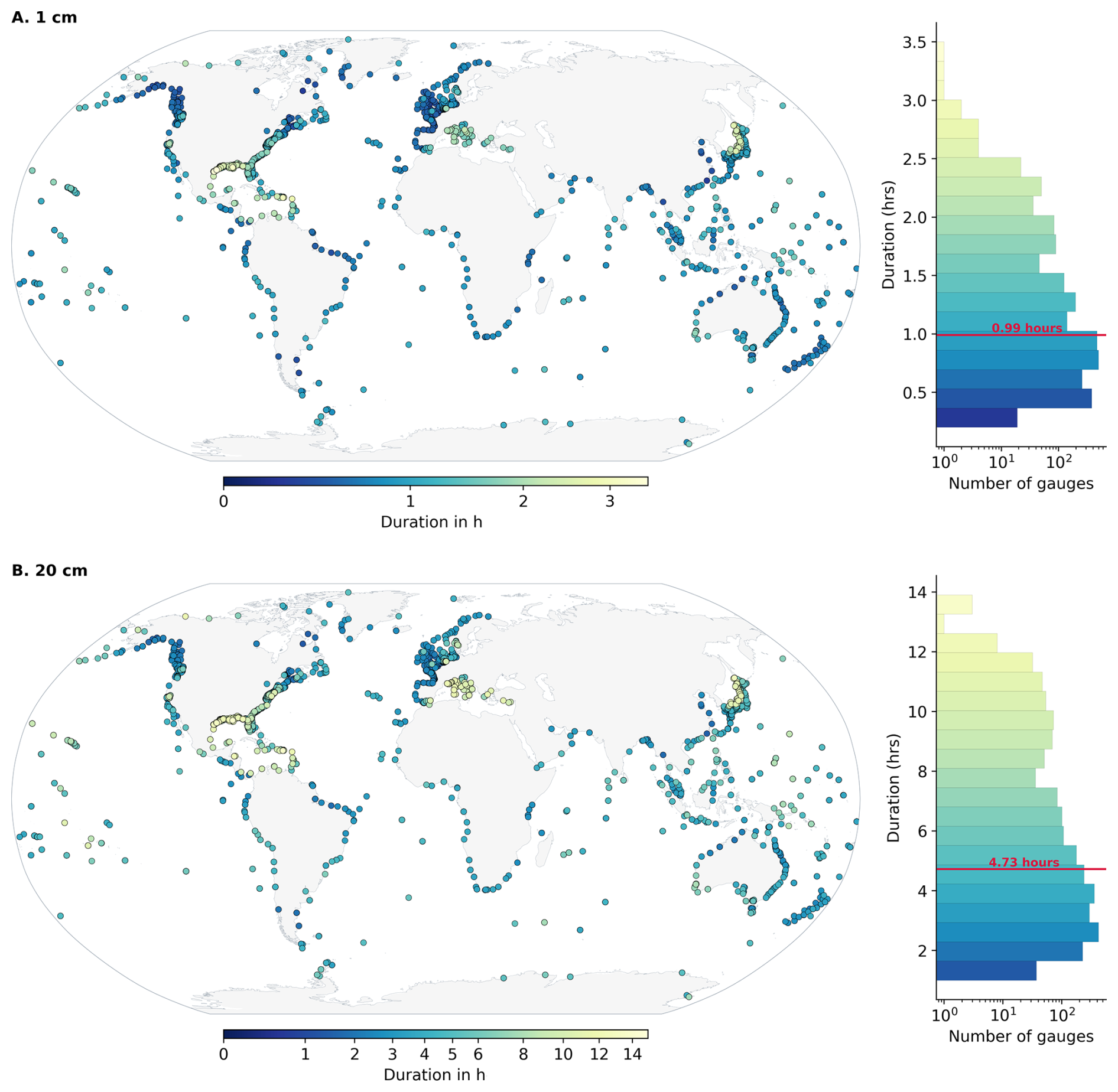
Figure 7 Water level duration within 1 cm (A) and 20 cm (B) thresholds from high tide. Some region plots are shown in Figs. B5 and B6. For (A) and (B), respectively, a histogram is presented to represent the distribution of durations across all tide gauges, with the red line indicating the mean duration.

Globally, the coastal tides evaluated stay within 1 cm of their peak from 0.2 to 3.5 h, with a mean of 1.0 h. The time spent within 20 cm of the peak varies from 1 to 14 h, with a mean of 4.7 h. The distribution of these durations within the selected thresholds is shown in Fig. 7, which demonstrates that despite these mean values (demonstrated in a line within the histogram), there is a strong variation in the duration hours spread globally. The duration near the peak matters for multiple reasons; for example, in regions subject to long high-water stands, waves may erode vulnerable shorelines for longer periods during storms. Additionally, tidal properties interact with storm surge to produce a composite wave; generally speaking, the longer the high-water stand, the longer the ensuing high-water period during a storm may be, given equal meteorological forcing. Ecological processes are often critically dependent on time out of water (emersion time) or time inundated. We note that the duration of mean tides, neap tides, and low-water periods may differ from the patterns shown in Fig. 7, and that some variability in tide duration (generally <10 %) will occur even between spring tides of the same magnitude, at a given location (Talke, 2025). This occurs because the mix of diurnal and semidiurnal tidal forcing, along with their phases, continually shifts. As shown in Talke (2025), the high or low water period that results can usually be represented as a sine wave with an amplitude and a period that is somewhere in between the main tidal bands. The resulting duration for a given inundation depth is directly proportional to this period.

A simple trigonometric identity explains that the duration of a tide near its peak (t_d) depends on the inundation depths, the amplitude of the tide above the mean water level (A), and the effective period of the sine wave that best represents each high water stand (see Talke, 2025 for a derivation):

$$\begin{array}{}\text{(5)}& {\displaystyle }{\displaystyle }{t}_{\mathrm{d}}={\displaystyle \frac{T}{\mathit{\pi }}}{\cos }^{-\mathrm{1}}\left(\mathrm{1}-{\displaystyle \frac{s}{A}}\right)\end{array}$$

For most locations, the amplitude of the high water stand (A) is driven primarily by the sum of the diurnal and semidiurnal band wave, with a correction for their relative phase; as tide amplitudes and relative phases vary over the synodic and tropical spring-neap cycles, the ratio $\frac{s}{A}$ (and thus duration) will correspondingly shift. Additionally, and perhaps surprisingly, the period T that best describes an individual high-water stand is typically neither semi-diurnal (12–13 h) nor diurnal (24–25 h), unless one band clearly dominates. Instead, as shown both empirically and theoretically by Talke (2025), the period T used in Eq. (5) is a composite of both tidal bands, but usually biased towards the semidiurnal frequency. For example, the superposition of a 0.64 m semidiurnal wave (12.4 h period) with a 0.46 m diurnal wave (24.8 h period, relative phase =0) will result in a composite wave with a period of 15 h (Talke, 2025). The duration of some high-water stands (<10 %) are not easily fit by a sinusoidal wave, particularly if amplitudes are small and the timing of diurnal and semidiurnal waves are significantly out of phase; moreover, the influence of quarter-diurnal constituents and other bands in shallow water remains to be elucidated (Talke, 2025). The variability of high-water stands between spring and neap tides and due to seasonal and longer-time scale variability remains to be elucidated, as does the duration of low-water time periods. Nonetheless, as shown here, significant global variability in the typical duration of a spring-high water period exists, driven by fundamental differences in the relative phases and amplitudes of the diurnal and semidiurnal constituent bands.

The superposition of a tide and surge wave can result in a composite sine wave, similar to what happens when a diurnal and semidiurnal wave are added, provided their peaks are not significantly phase shifted, and the surge can be approximated near its peak by a sine wave (see e.g. Familkhalili et al., 2020). Under these conditions, Eq. (5) can approximate the duration of the storm-tide above a threshold, and provide insights into the processes driving flood duration. As with tidal bands, theory and empirical analysis suggest that the resulting storm-tide amplitude A depends on the individual amplitudes and relative phases of the tide and storm surge. Additionally, the period T of the storm tide wave used in Eq. (5) is a composite of the two frequencies, but biased towards the smaller period wave (see Talke, 2025). Additional non-linearities related to phase speed and frictional non-linearities may additionally affect this analysis, and more work is warranted to empirically assess storm-tide durations.

The effects of relative sea-level rise on future tidal flood duration for the USA are explored by Talke (2025), with results suggesting that the time-scale to transition from a zero to two-hour high-tide flood varies from 1 to nearly 100 years. Future research can build on the results shown here to evaluate how tide-induced flooding events could evolve as a result of local sea-level changes, tidal trends, and other forcing factors, including wind and river flow.

7 Tidal changes

It is well understood that tidal characteristics have changed over long geological time scales, driven by tectonic processes (which alter the size, depth, and shape of the ocean which in turn impacts tidal propagation and resonance) and changes in Earth's rotation (tidal friction gradually slows Earth's rotation, lengthening the day and modifying the tidal frequencies and their resonance with ocean basins). However, over much shorter time periods of the last few hundred years, and perhaps because of the reliability of tide predictions, casual observers often assume that tidal constituents are stationary, because planetary orbital motions are stable and predictable. Nonetheless, it has been observed that tidal levels in many locations change considerably due to non-astronomical factors over seasonal, decadal, and secular time scales (Doodson, 1924). In their comprehensive review, Haigh et al. (2020) synthesise global evidence that tides are changing due to non-astronomical factors, documenting widespread regional trends in tidal amplitudes and constituent behaviour across the 19th to early 21st centuries (see also the review of Talke and Jay, 2020). They identify six principal local-scale drivers (such as bathymetric change, river discharge, and anthropogenic alteration) and eight broader regional/global mechanisms (including sea-level rise, ice-sheet collapse, and ocean stratification) that influence tidal variability. While attribution is challenging because coastal tidal signals reflect the integrated effects of local, regional, and ocean-basin-scale influences, modelling studies reviewed indicate that future sea-level rise and changes in coastal morphology will continue to alter tidal regimes, with significant implications for coastal hazard assessment, ecosystem change, and infrastructure design.

To evaluate tidal changes observed from tide gauges, we calculated yearly amplitudes of the M₂ and S₂ tidal constituents and derived a trend relative to the TICON-4 amplitude estimations. Yearly amplitude trends were estimated by fitting an ordinary least squares linear regression to the annual amplitude values, after excluding values outside one standard deviation from the median. To account for any potential temporal autocorrelation in the tide gauges, we utilized Newey-West Heteroscedasticity (Newey and West, 1987) and autocorrelation-consistent standard errors. The trend was quantified as the mean annual change in the fitted values. The uncertainty was estimated as the mean width of the 95 % observation confidence interval from the adjusted regression predictions. In the provided dataset, the trend and the uncertainty for each constituent are provided. However, in Fig. 8, the trends are only shown when the trend exceeds the uncertainty value, with the gauge marked with a small white dot when this is not the case.

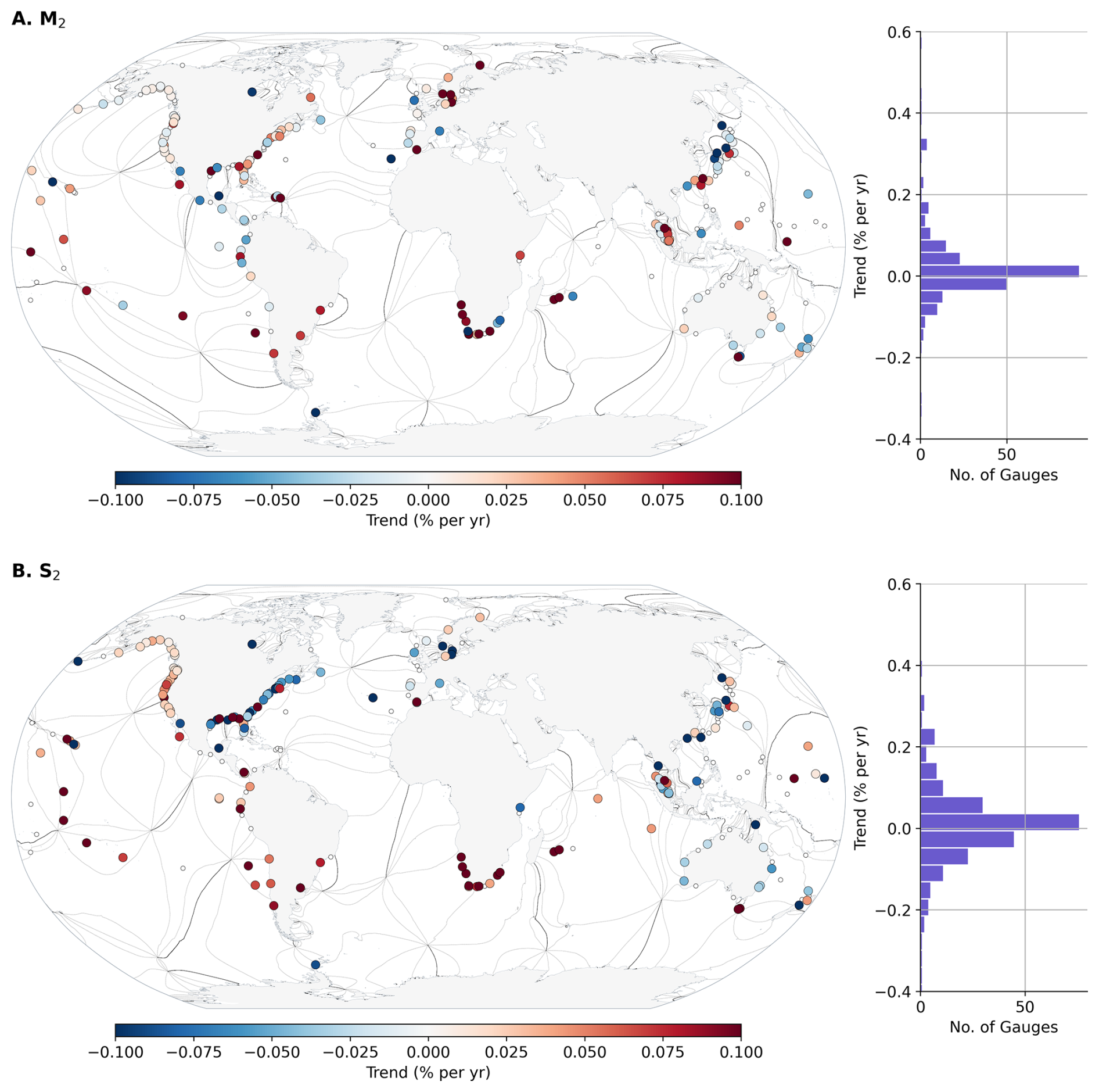
Figure 8 M₂ and S₂ amplitude percentage trend derived from UHSLC research quality tide gauges with at least 30 years of observations. The black contour lines are the phase lag of the respective constituents obtained from FES2022.

This analysis focuses solely on gauges with more than thirty years of observations from the UHSLC research-quality (UHSLC-RQ) database, resulting in a total of 237 tide gauges. The use of one data source also prevents any duplicated tide gauges being used, which could bias any mean or median statistics presented below. The thirty-year threshold is selected to minimize any correlation with possible non-equilibrium nodal modulations that are known to occur at some gauges (Feng et al., 2015). The results are shown in Fig. 8.

Our analysis found that for both constituents, 52 % and 53 % of tide gauges showed a statistically significant (defined as when the amplitude trend exceeds the estimated uncertainty) trend for the M₂ and S₂ tide, respectively. For the M₂ tide, the trends are positive in 58 % of the tide gauges, with a mean absolute trend of 0.19±0.11 mm yr⁻¹ and ranging from −1.47 to 1.80 mm yr⁻¹. For the S₂ tide, the trends are positive in 54 % of tide gauges, with mean trending being 0.10±0.05 mm yr⁻¹, ranging between −1.17–0.98 mm yr⁻¹.

Tidal trends can be observed in both constituents, with their directions varying regionally. It is expected that the observed trends between M₂ and S₂ would be different due to their different astronomical forcings: roughly 15 % of S₂ is radiational (Arbic, 2005). Of the 237 gauges, 62.4 % of tide gauges exhibit consistent trend directions between the M₂ and S₂ amplitudes. In several regions, such as South Africa and the east and western coasts of America, these trends are largely coherent or consistent, but it can be observed that certain tide gauges do not conform to the trends expressed by nearby gauges, e.g. in the Gulf of Mexico and Japanese tide gauges.

Anomalous trends can result from a variety of factors, ranging from malfunctioning instrumentation to measurements nominally correct but somehow affected by localized tidal effects unrepresentative of the surrounding sea (Woodworth, 2010). Measurement errors, such as elevations corrupted by biofouling or silt buildup, can build up slowly enough to impact amplitudes and/or phases over months or even years (depending on gauge maintenance), and they can thus affect estimated trends. Similarly, environmental changes such as the daily heating and cooling of the gauge can affect some constituents if not properly accounted for (e.g. acoustic gauges are known to be sensitive to environmental temperatures affecting sound speed; Hunter, 2003); these kinds of errors tend to turn up when instrumentation changes and can thus induce small errors over long periods.

Other anomalous tidal trends reflect correct physical measurements but of a localized nature. A prime and common example is a change in tide following harbor renovations or following nearby dredging for navigational purposes. In fact, one of the largest amplitude trends in North America (of 1.6 mm yr⁻¹) occurs at Wilmington, North Carolina (Flick et al., 2003) and is likely the result of dredging in the Cape Fear River (Familkhalili and Talke, 2016). Such river effects are not easily eliminated from our data, since so many tide gauges have historically been located in or very near rivers because of their obvious importance to navigation. Tide gauges impacted by tectonic or other vertical land motions can be especially problematic for determining sea-level trends, but they usually have little impact on tidal trends. More common and more problematic, however, is any horizontal relocation of the gauge, even over short distances. For example, Ray and Talke (2019) discuss the tide gauge at Portsmouth, New Hampshire, which has a favorably long time series (beginning in 1926) but is spoiled by repeated relocations at different spots around Seavey Island (in the Piscataque River between Maine and New Hampshire), subsequently moved in 2003 farther downstream; these repeated relocations, some of them unreported, hamper any attempt at trend estimation.

These challenges in deriving tidal trends, which, as shown here, are of very small magnitudes, are not limited to tide gauges, as efforts to derive such trends from satellite altimetry are also susceptible to a large number of different errors, some of them very difficult to mitigate (see Ray and Schindelegger, 2025, for more information).

For the S₂ tide, clear region-specific changes in the tides can be observed, particularly positive trends on the west coast of America of 0.07±0.02 mm yr⁻¹, with negative trends of on average $-\mathrm{0.08}\pm \mathrm{0.03}$ mm yr⁻¹ are observed on the eastern coast, which agrees with the earlier findings (Jay, 2009; Ray, 2009; Woodworth, 2010). Our analysis shows that tide gauges in Southern Africa exhibit the largest variations in tidal amplitudes across both the M₂ and S₂ tides (Fig. 8) of 0.39±0.25 mm yr⁻¹ and 0.30±0.16 mm yr⁻¹ respectively, particularly for long-term gauges located in harbours or estuaries (the Knysna tide gauge, located in an estuary in South Africa, exhibits the largest calculated M₂ trend, 1.80±0.2 mm yr⁻¹),, where tidal statistics measurements are susceptible to local changes dredging, land reclamation, and other geometric changes (Haigh et al., 2020; Talke and Jay, 2020).

8 A note on river tides

Tides in rivers, deltas, and estuaries are greatly influenced by river flow, geometry, and shallow water effects (e.g. Le Provost, 1991; Kästner et al., 2019; Hoitink and Jay, 2016). The complex nonlinear interactions between tides, river flow, and shallow-water topography mean that using the harmonic method may be insufficient to provide in-depth characterizations of tidal characteristics within rivers. Multiple methods have been developed to characterize river-tide interactions, such as the response-based RTide approach (Monahan et al., 2025), a modified harmonic analysis approach that includes non-stationary effects (NSTIDE; Matte et al., 2013) and the continuous wavelet transform method (CWT_Multi; Lobo et al., 2024). However, a global dataset of river tide gauges is currently unavailable within GESLA-4, though river and deltaic systems within some countries (such as the US, the Netherlands, and Germany) are reasonably well-covered. An effort to characterize river tides globally, similar to this effort, would clearly be of high value to the community, especially considering the importance of these systems to communities (Hart-Davis et al., 2026a; Beemster et al., 2026). Our synthesis motivates such an effort, but is beyond the scope of this current work.

9 Concluding remarks

This manuscript provides a global analysis of tidal characteristics based on tide gauge observations. We revisited established methods such as tidal range and form factors, which, thanks to the extended efforts of GESLA-4, have been applied to additional regions along global coasts. Additionally, we have provided updated perspectives on tidal changes across the coasts as well as for the first time, a global assessment of the duration of high-water periods. The latter statistic provides a new perspective on the potential of compound flooding across the ocean, and can be particularly useful for coastal management efforts. The insights we provide highlight the importance of the continued efforts to maintain these high-quality datasets for tidal research. Beyond ocean tides, the maintenance of these tide gauge records is critical for detecting and understanding changes in sea level, both in the context of sea level rise as well as for extremes such as flooding events (Haigh et al., 2022).

Throughout the figures of this manuscript, it is evident that there are significant gaps in the global coastal coverage, particularly in the global South. While some of this may be due to governmental restrictions, a significant portion of the issue stems from the lack of capacity and finances to not only deploy but also maintain tide gauges. Cost-effective initiatives are starting to grow (Mydlarz et al., 2024), and making these widely available could assist in helping to fill the gaps in the observing system. Additionally, it is clear from the available observations that a knowledge gap exists in the characterization of river tides. This is largely due to the lack of a harmonized dataset of river measurements, such as GESLA-4, and to the challenge of presenting non-stationary tidal statistics in such a global analysis. Conducting such an analysis on river tide characteristics would certainly be a highly valuable resource for the community.

Although satellite observations provide suitable coverage of ocean tides, it is essential to emphasize that tidal research relies on tide gauge observations to continue our understanding of tidal variability across the global oceans. They complement altimetry by providing invaluable “ground truth”, by allowing assessments of long-term changes, and by revealing fine-scale details of the tidal spectrum.

Further gaps are evident in the polar coastal oceans, largely due to the challenges of maintaining measurement equipment in these regions, which are characterized by harsh environments and remoteness. Global navigation satellite systems (GNSS) reflectometry is a new evolving technology for measuring sea level which has a huge potential in polar regions (Larson et al., 2013). The strengths are mainly that the infrastructure consisting of the GNSS and coastal continuously operating reference stations (CORS) may be re-used as a remote sensing technique. No additional equipment mounted in the water is required, which is especially beneficial in harsh environments. Efforts are ongoing to explore the incorporation of GNSS reflectometry in tidal research, particularly in the polar regions (Tabibi et al., 2020), which will help provide further coverage in the future.

Ocean bottom pressure sensors are important sources of in-situ measurements of tidal characteristics in the global oceans (Ray, 2013), providing greater coverage, including in higher latitudes (Hart-Davis et al., 2024). However, globally available datasets of GNSS-R and ocean bottom pressure sensors applicable for such an analysis, as presented in this study from GESLA-4, do not currently exist. As these measurements continue to be collected, a public archive of these data will be useful for further investigating ocean tides on a global scale. Finally, there are still a large number of sea level records available around the world in paper-based format (Talke and Jay, 2013; Talke et al., 2013; Pouvreau, 2008; Bradshaw et al., 2015; Latapy et al., 2023). Finding and digitising these records, however, remains a difficult and time-consuming endeavor.

Appendix A:  

To construct the admittance matrix used for tidal inference, we assume a linear admittance based on several pivot tides from TICON-4. We exclude tides that have a significant radiational component (e.g. S₁, S₂, R₃, …) as pivot tides. Admittance is separately applied for degree-3 tides contained in TICON-4 (³N₂, ³L₂, M₃) which implicitly estimate 9 tides from Hartmann and Wenzel (1995), increasing the total number of tides to M=159 (Fig. A1) Further, the tide-raising forces are explicitly corrected for the FCN-resonance that disturbs the tide-raising forces for the K₁ tidal group. Based on the admittance matrix, tidal heights are computed according to the formula

$$\begin{array}{ll}{\displaystyle }\text{Tide}=& {\displaystyle }\sum _{i=\mathrm{1}}^N\left(\sum _{j=\mathrm{1}}^M{A}_{ij}\cos [{\mathit{\omega }}_{j}t+V_j]\right)H_i\cos \left(G_i\right)\\ \text{(A1)}& {\displaystyle }& {\displaystyle }+\sum _{i=\mathrm{1}}^N\left(\sum _{j=\mathrm{1}}^M{A}_{ij}\sin [{\mathit{\omega }}_{j}t+V_j]\right)H_i\sin \left(G_i\right).\end{array}$$

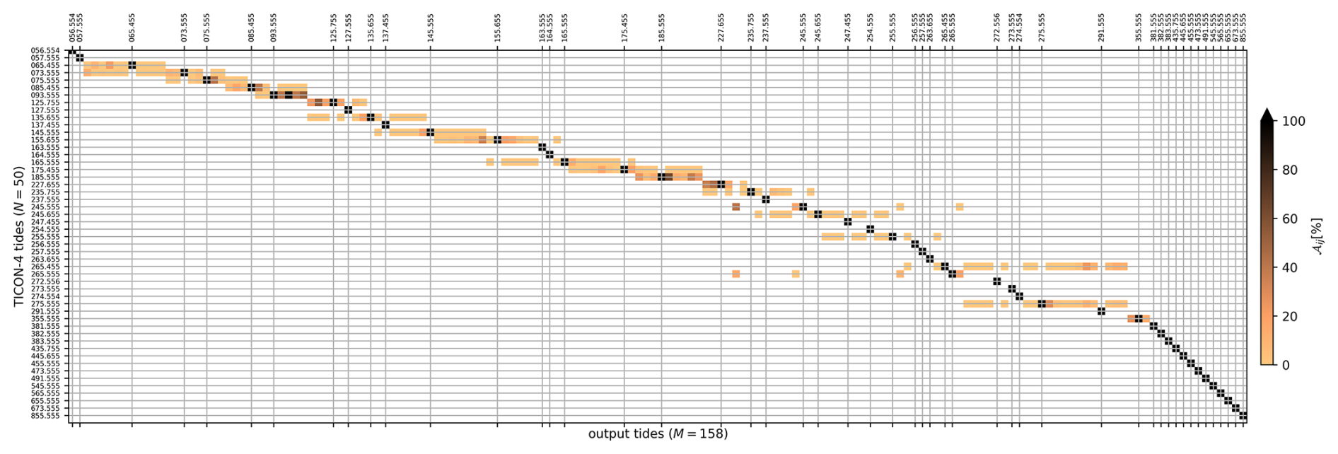
Figure A1 Admittance matrix employed within this study in %. The section describing degree-3 admittance (red) is marked out. Radiationally-contaminated tides and shallow-water tides are disallowed as pivot tides (e.g. S₁: 165.55 and M₄: 455.555). TICON-4 tides are labeled with their Doodson codes on the input and output sides of the matrix.

A numerical advantage of this formula is that the computation of the sum over j is independent of the respective tidal constituents, i.e. it has to be only computed once for all tide gauges. Furthermore, the construction A_ij can be easily tailored to the desired level of accuracy, ranging from using a unit matrix to lowering the threshold to an arbitrarily low level. Additional information, including examples of admittance matrices for satellite gravimetry and software for computation, can be obtained from https://www.tugraz.at/institute/ifg/downloads/ocean-tides, last access: 6 May 2026.

To evaluate this approach with a more commonly used method, we compared tidal heights predicted from the perth5 software (Ray, 2025, https://codeberg.org/rray/perth5, last access: 6 May 2026) and present differences between them for the large tide observed at the Brest tide gauge; see Fig. A2. The total variance difference between these two approaches is 1.91 cm² (median difference of 1.22 cm), a small fraction of the signal variance at Brest, which is approximately 25 000 cm².

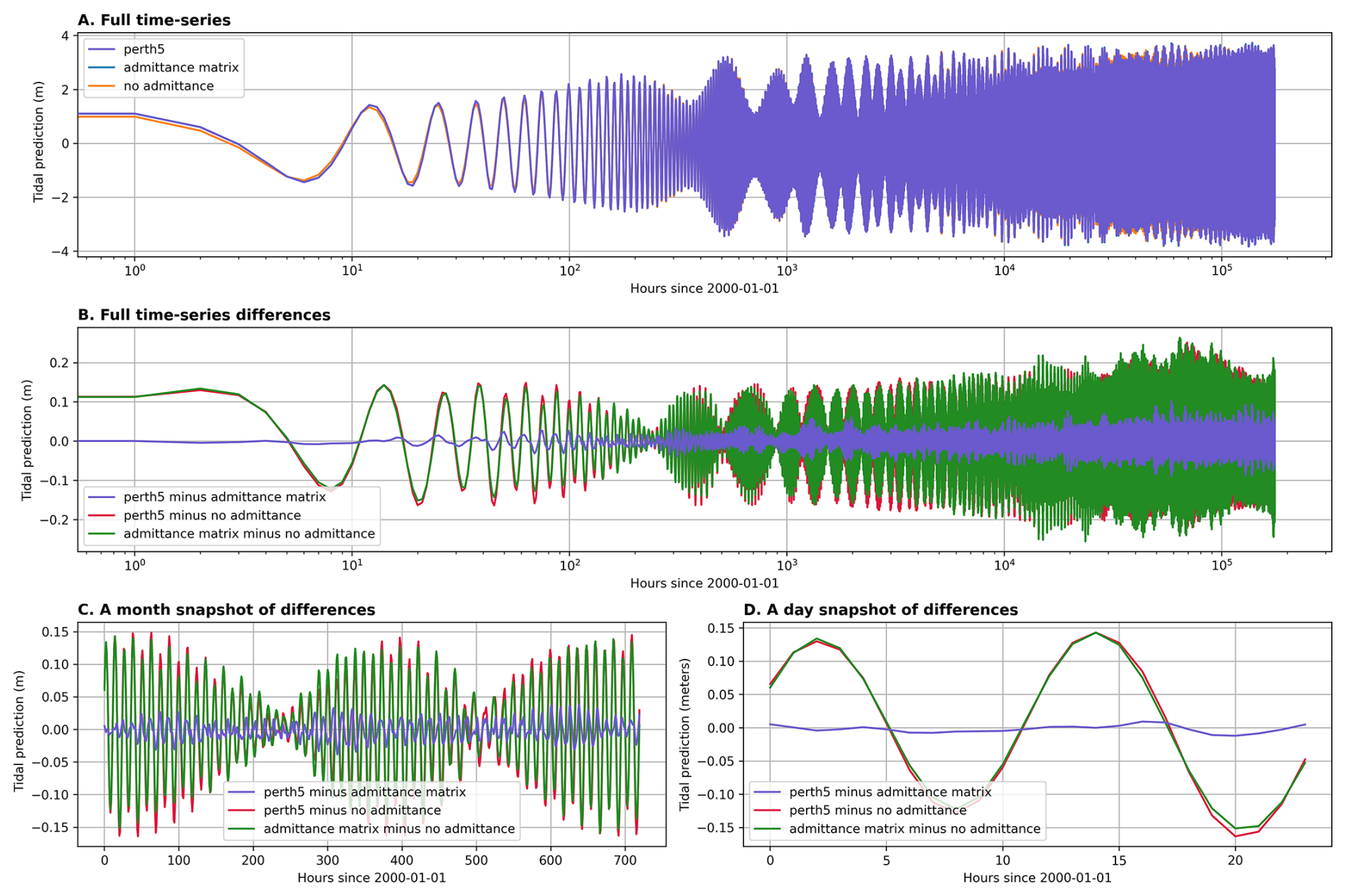
Figure A2 Comparison of tidal predictions made by the methods presented in Appendix A with and without admittance, and the perth5.f software. (A) presents a 20-year prediction by the three methods, with differences between the methods across the full time-series (B) as well as a month (C) and day (D) snapshot also shown.

Appendix B:  

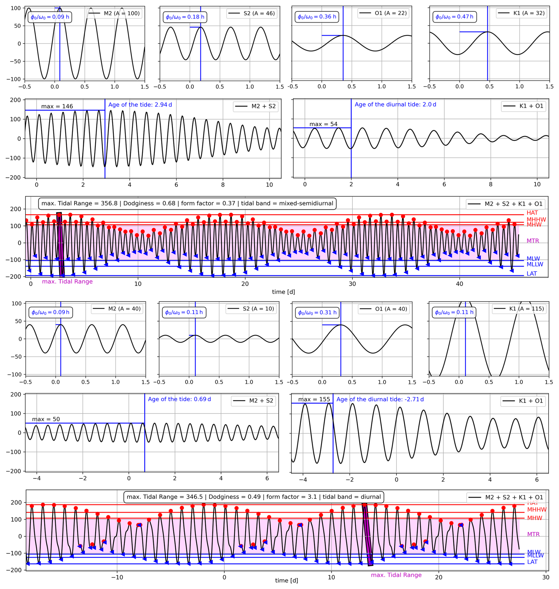
Figure B1 Top: Sea surface height time series for four major tides (M₂, S₂, K₁, O₁) with the local phase shift ϕ₀ indicated. The amplitude ratio between M₂ and S₂ (100:46), as well as the ratio between K₁ and O₁ (32:22), approximates the respective ratios in the TGP. Second Row: Resulting semidiurnal (M₂+S₂) and diurnal (K₁+O₁) time series indicating the age of the tide, i.e. the maximum constructive interference after t=0, where diurnal and semidiurnal forcing are maximum. Third row: Tidal time series as a consequence of all 4 tides with maxima (red) and minima (blue) indicated. Additionally, the tidal datums and some tidal characteristics introduced in the text, e.g. the maximum and mean tidal ranges (purple), are indicated. The lower half of the figure shows the same information for a diurnal tidal regime, dominated by K₁, exhibiting a negative age of the diurnal tide. Heights are given in arbitrary units.

Table B1 A summary of the statistics presented in this manuscript. Additional information on these characteristics can be found in Doodson and Warburg (1941), Pugh and Woodworth (2014).

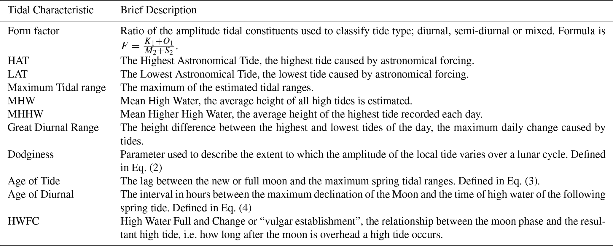
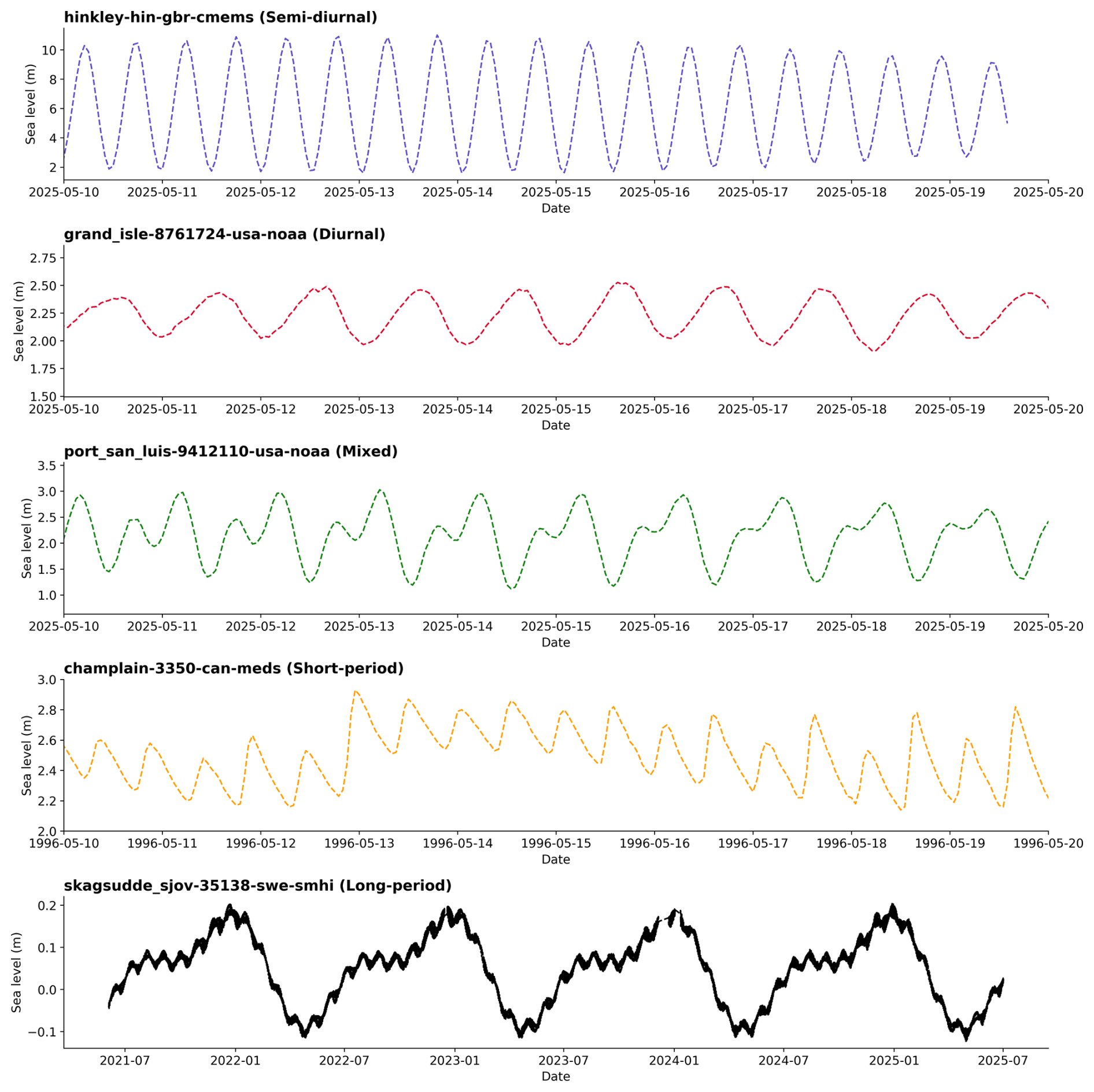
Figure B2 Time series of tide gauge data within each tidal band, as discussed in Fig. 4. For the long-period example, non-tidal variability has been removed to highlight only the tidal contributions.

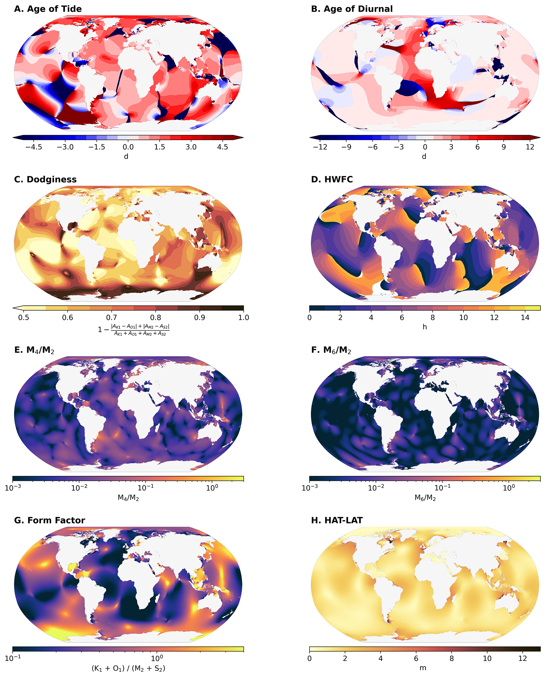
Figure B3 For comparisons to the results seen in the tide gauges, model results derived using FES2022 Lyard et al. (2021, updated).

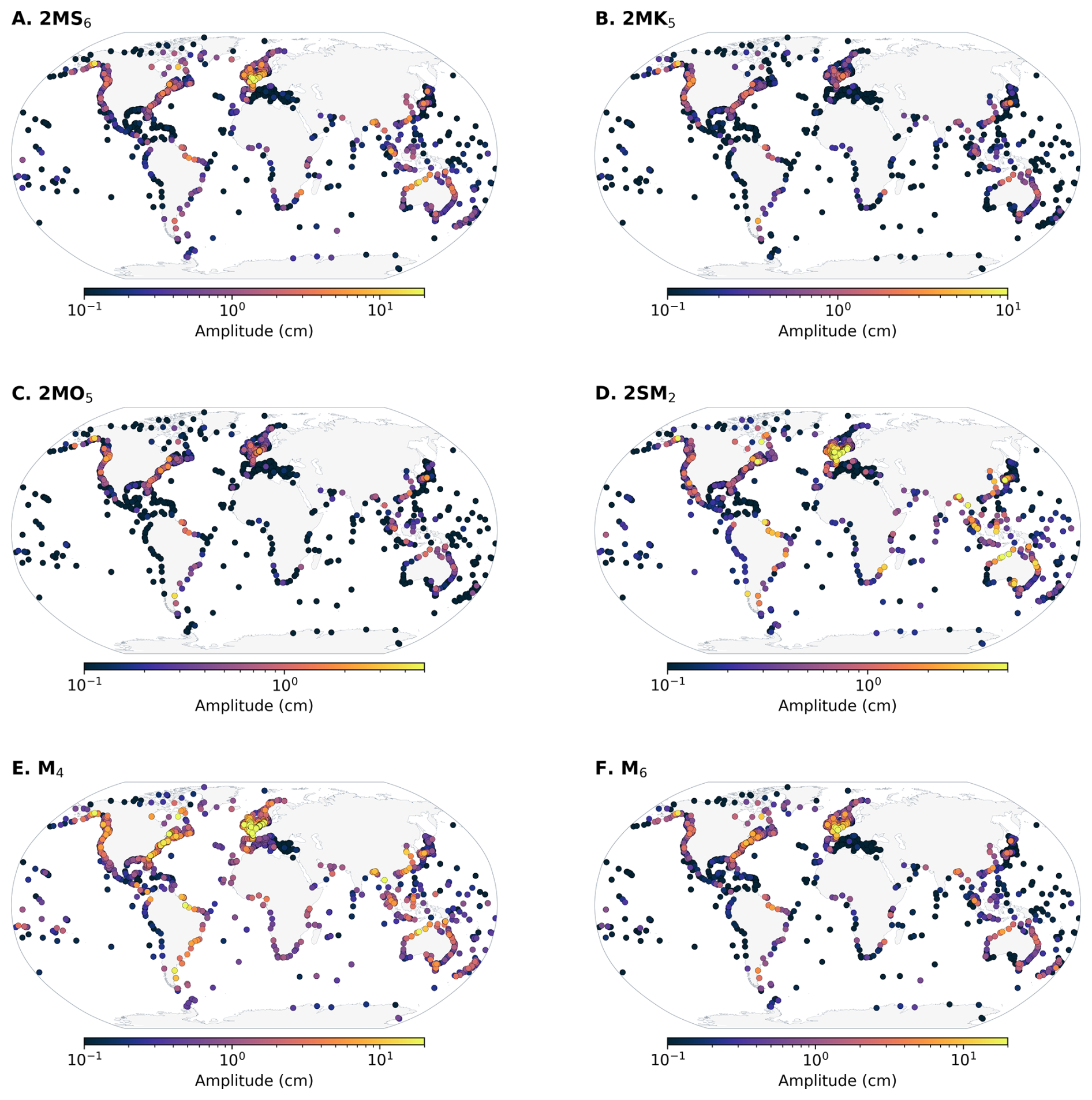
Figure B4 Shallow water tidal constituents taken from TICON-4.

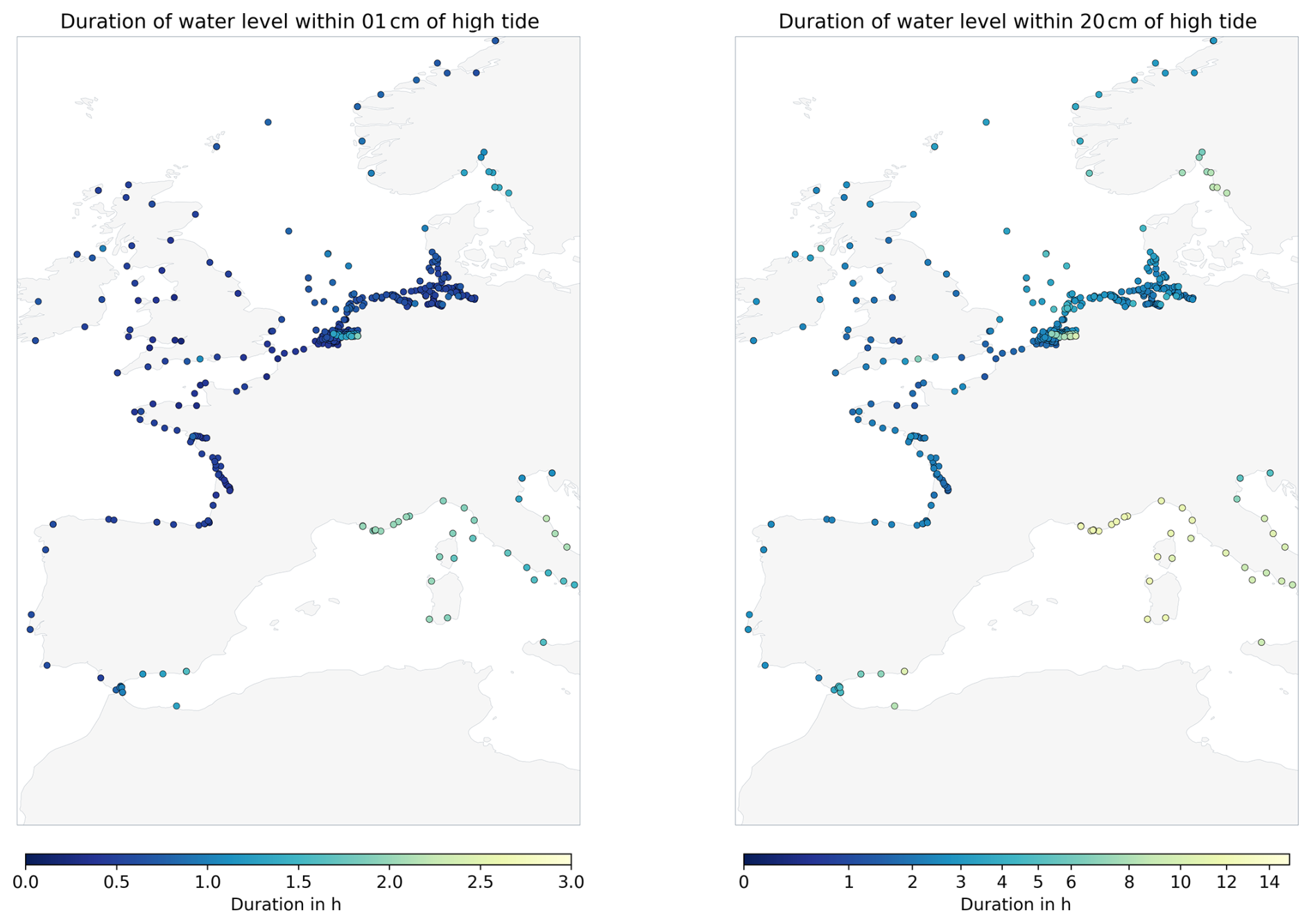
Figure B5 European coastal subset of the flood timing extent.

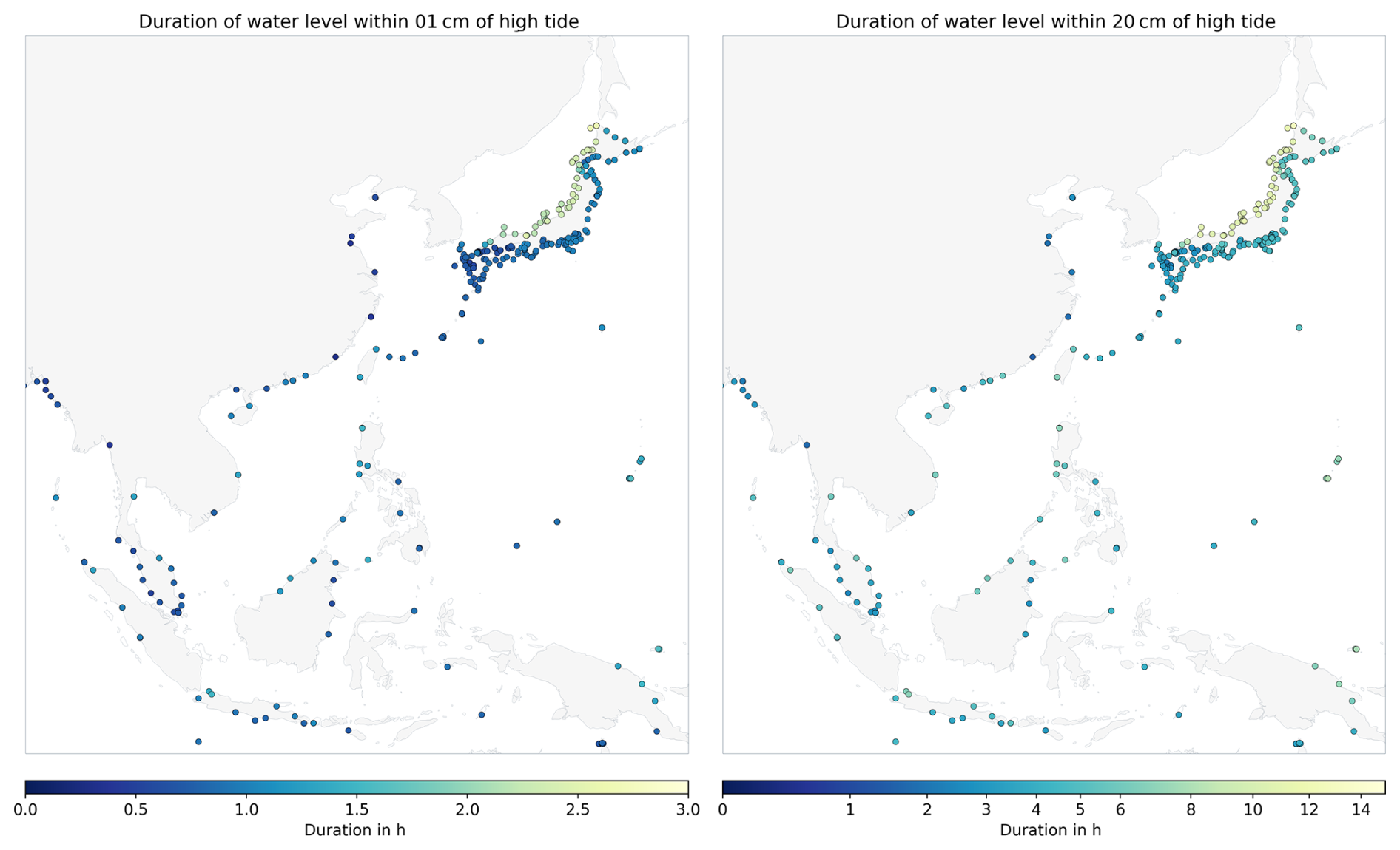
Figure B6 South-east Asian subset of the flood timing extent.