Ocean salinity across space-time scales: from water cycle indicator to dynamical driver

Ocean salinity plays a complementary role in the climate system: it integrates changes in the global water cycle while also helping drive ocean circulation through its control on seawater density. Salinity has long been viewed as the ocean's “rain gauge”, a largely passive recorder of surface evaporation, precipitation, and runoff. Yet salinity also shapes the currents and mixing that redistribute heat and freshwater, raising a central question: when does salinity mainly record climate forcing, and when does it actively influence climate dynamics? This review synthesizes two decades of satellite and in situ observations within a regime-dependent framework in which salinity's function is set by the competition among freshwater forcing, advection, and mixing timescales. At basin scales (> 1000 km) over decades, salinity tracks water-cycle change through pattern amplification, with fresh regions freshening and salty regions becoming saltier. At regional to mesoscale (∼ 10–500 km) and seasonal-to-interannual timescales, salinity traces circulation pathways; subsurface anomalies often reflect subduction and ventilation histories from years earlier. At submesoscales (O(10 km)) and synoptic timescales (hours to days), salinity becomes dynamically active, sharpening density fronts, modulating stratification, and altering mixing in ways that feed back on its own transport and air–sea exchange. Understanding ocean climate response requires resolving regime boundaries where these balances shift. The critical observational gap is global sea-surface salinity at O(10 km), where salinity transitions from passive tracer to active driver yet current satellite products cannot resolve this scale. Observations at regime boundaries would show how water-cycle intensification and ocean circulation changes interact, improving projections of climate change, ocean heat storage and distribution, and ecosystem dynamics at regional and global scales.

1 Introduction

Ocean salinity occupies a unique position at the nexus of the global water cycle and ocean circulation. As the integrated expression of surface freshwater fluxes (evaporation, precipitation, river discharge, and ice melt), salinity has long been viewed as the ocean's natural rain gauge, faithfully recording the changes in Earth's hydrological cycle (Dickson et al., 1988; Curry et al., 2003; Boyer et al., 2005; Durack and Wijffels, 2010; Helm et al., 2010; Skliris et al., 2014; Vinogradova and Ponte, 2017; Cheng et al., 2020; Yu et al., 2020). Yet through its fundamental role in setting seawater density alongside temperature, salinity also actively shapes ocean stratification, convection and mixing, and governs large-scale circulation (Talley, 2008; Mignot and Frankignoul, 2010; Schanze et al., 2010; Kolodziejczyk and Gaillard, 2013). This dual character of being both passive recorder and active driver raises a fundamental question: under what conditions does salinity reflect climate forcing, and when does it shape climate dynamics? This review synthesizes how observational advances over the past two decades have revealed that the answer depends critically on spatial and temporal scale, with salinity's role emerging from the competition among forcing, advection, and mixing processes.

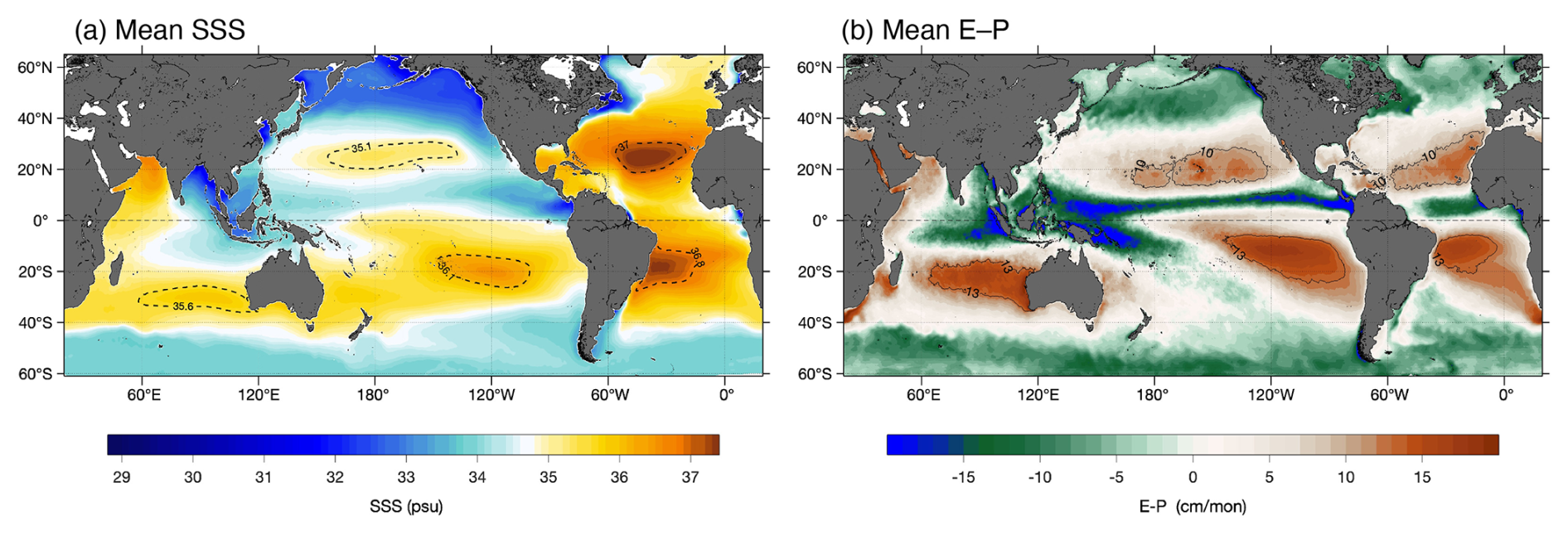
Figure 1 Time-mean fields. (a) sea surface salinity (SSS) and (b) evaporation minus precipitation (E−P) averaged over 2012–2022. SSS is from OISSS monthly 0.25° product (Melnichenko, 2023), E from OAFlux monthly 0.25° analysis (Yu, 2019), and P from GPCP Monthly 0.5° v3.2 (Huffman et al., 2023). Adapted from Yu (2023).

The traditional “rain gauge” perspective treated salinity as a passive consequence of atmospheric forcing in which net precipitation regions freshened, net evaporation regions became more saline, and water cycle processes left their signature on surface and subsurface patterns (Warren, 1983; Schmitt, 2008). This framework enabled insights into global water balance (Baumgartner and Reichel, 1975) and paleoclimate reconstruction (Rohling and Bigg, 1998). The apparent correspondence between ocean salinity and evaporation-minus-precipitation (E−P) motivated attempts to infer water cycle variations from salinity observations (Gordon and Giulivi, 2008; Yu, 2011; Terray et al., 2012; Durack et al., 2012; Skliris et al., 2016; Vinogradova and Ponte, 2017; Fournier et al., 2023). Implicit in this framework was a largely one-way causality in which atmospheric forcing determined salinity, and salinity served primarily as a marker of forcing variability, with limited consideration of feedbacks through ocean circulation.

This passive view neglects a fundamental reality: salinity anomalies do not remain where they are forced. They are advected by ocean currents, modified by mixing, and, through their impact on density, feed back on the circulation that transports them. High-latitude freshening can inhibit deep convection, weaken the meridional overturning circulation, and alter basin-scale heat transport (Rahmstorf, 1995; Barreiro et al., 2008; Holliday et al., 2020), while tropical freshening strengthens near-surface stratification, reduces vertical mixing, and modifies upper-ocean thermal structure (Lukas and Lindstrom, 1991; Maes et al., 2002; Mignot et al., 2012; Camara et al., 2015). In evaporative subtropics, persistent E−P excess combined with Ekman convergence maintains subtropical salinity maxima (Qu et al., 2013; Gordon et al., 2015; Bingham et al., 2019; Aubone et al., 2021); subduction of these waters ventilates mode waters and shallow overturning cells, exporting surface freshwater anomalies to the interior and equatorward (Qu et al., 2016; Yu et al., 2018; Zika et al., 2018). At submesoscales, salinity becomes equally important as temperature in driving density gradients, shaping stratification and mediating vertical exchange near surface (Rudnick and Ferrari, 1999; Timmermans and Winsor, 2013; Jaeger and Mahadevan, 2018; Coadou-Chaventon et al., 2024; Yu, 2026). Unlike temperature, salinity variations lack strong restoring feedbacks, as freshwater fluxes force salinity anomalies but do not rapidly relax them, making salinity variations both more persistent and more strongly shaped by advection and mixing than their temperature counterparts (Yu, 2011; Vinogradova and Ponte, 2013; Lyu et al., 2025). The competition among forcing, advection, and mixing timescales determines whether salinity behaves primarily as a rain gauge recording atmospheric forcing, a passive tracer marking circulation pathways, or a dynamical driver actively modifying ocean stratification and currents.

Over the past two decades, observational advances have transformed our ability to characterize salinity's scale-dependent roles systematically. The Argo program, with thousands of autonomous profiling floats sampling temperature and salinity in the upper 2000 m, provides near-real-time monitoring of subsurface variability (Roemmich and Gilson, 2009; Riser et al., 2016), while historical ship-based compilations provide century-long context for sea surface salinity changes (Bingham et al., 2002; Boyer et al., 2005; Ishii et al., 2006; Good et al., 2013; Friedman et al., 2017). In parallel, satellite salinity missions, including ESA's Soil Moisture and Ocean Salinity (SMOS) (2009–present) (Reul et al., 2012), NASA's Aquarius (2011–2015) (Lagerloef et al., 2013), NASA's Soil Moisture Active Passive (SMAP) (2015-present) (Entekhabi et al., 2010), and the Chinese Ocean Salinity Mission (COSM) (2024–present) (Zhang et al., 2018) have provided continuous, near-global sea surface salinity (SSS) that resolves mesoscale features, tracks seasonal to interannual variability, and reveals the surface imprint of water cycle forcing (Vinogradova et al., 2019; Reul et al., 2020; Boutin et al., 2021). The emerging autonomous uncrewed surface vehicles (Saildrones, Wave Gliders, etc) in recent years have extended high-resolution salinity sampling to regions undersampled by Argo and ships, capturing submesoscale to mesoscale variability along extended trajectories (Patterson et al., 2025). Together, in situ and satellite salinity observations capture the spatial structure linking evaporation-precipitation patterns to surface salinity (Fig. 1). The large-scale correspondence between E−P and SSS, evident in the subtropical salinity maxima and tropical fresh pools, confirms the fundamental water balance relationship while revealing important regional departures driven by circulation and mixing. These observations, together with satellite measurements of terrestrial water storage from GRACE and GRACE FO (Tapley et al., 2004) and river discharge from SWOT (Morrow et al., 2019), form a global water cycle observing framework spanning the land-ocean-atmosphere continuum (Vinogradova et al., 2025).

These observations reveal salinity's scale-dependent dynamics and climate feedbacks. At basin scales, the amplification of mean patterns (fresh regions freshening, salty regions salinifying) confirms water cycle intensification (Durack and Wijffels, 2010; Helm et al., 2010; Durack et al., 2012; Skliris et al., 2016; Cheng et al., 2020; Yu et al., 2021), extending to semi-enclosed basins where evaporative loss drives coordinated salinity and bottom pressure changes (Lehmann et al., 2022; Liu et al., 2025). Basin-scale synchronization between subtropical maxima and tropical minima demonstrates coupling through circulation rather than local forcing alone (Hasson et al., 2018; Yu, 2023), while subsurface extremes reveal ventilation pathways throughout the water column (Skliris et al., 2014; Zika et al., 2015). Beyond recording water cycle change, salinity drives critical climate feedbacks: upper-ocean stratification changes modulate heat uptake and surface warming (Zika et al., 2018; Liu et al., 2023; Vogt et al., 2025), near-surface salinity anomalies predict continental precipitation (Li et al., 2016; Rathore et al., 2021), barrier layers intensify tropical cyclones (Balaguru et al., 2020), and high-latitude freshening weakens the Atlantic meridional overturning circulation (Caesar et al., 2018), with ecosystem and biogeochemical consequences across all scales (Fournier et al., 2023; Röthig et al., 2023).

Understanding these feedbacks matters for climate prediction and projection. Inadequate representation of salinity feedbacks could bias regional climate projections, while salinity's potential for nonlinear responses (Rahmstorf et al., 2005; Weijer et al., 2019) raises questions about model's capability to capture climate trajectories. Conversely, salinity observations may provide predictive information for seasonal-decadal forecasting (Qu et al., 2014; Zhu et al., 2014; Hackert et al., 2020). Quantifying salinity's scale-dependent roles has direct consequences for interpreting observed climate variations, constraining model biases, and projecting regional climate change.

This review synthesizes two decades of observations into a regime-dependent framework for ocean salinity behavior. Section 2 reviews the observational foundation from satellites, Argo, and historical archives that enables systematic characterization of salinity variability. Section 3 examines where and when salinity records water-cycle change: basin-scale and multi-decadal patterns where forcing dominates, mesoscale and seasonal-to-interannual redistribution where circulation shapes pathways, and submesoscale and synoptic dynamics where salinity actively shapes mixing and stratification. Section 4 develops a unifying framework showing how competition among forcing, advection, and mixing timescales determines these regime transitions, with implications for predictability and future projections. Section 5 identifies observational priorities at regime boundaries, particularly sustained global sea-surface salinity at O(10 km) resolution, to constrain how water-cycle intensification couples with circulation change under warming.

2 Observational foundations: resolving scale-dependent salinity dynamics

Observing salinity's scale-dependent dynamics requires capturing the spatial and temporal scales where forcing, advection, and mixing compete. Basin-scale patterns demand decadal stability and global coverage to detect water cycle trends. Mesoscale circulation pathways require spatial continuity to resolve how anomalies propagate and organize. Submesoscale dynamics require high-frequency temporal sampling to capture processes modifying stratification and mixing. No single observing platform spans basin-to-submesoscale spatial resolution (1000 to 1 km) while maintaining decadal-to-synoptic temporal coverage (decades to hours), necessitating integration across complementary systems designed for specific scale regimes.

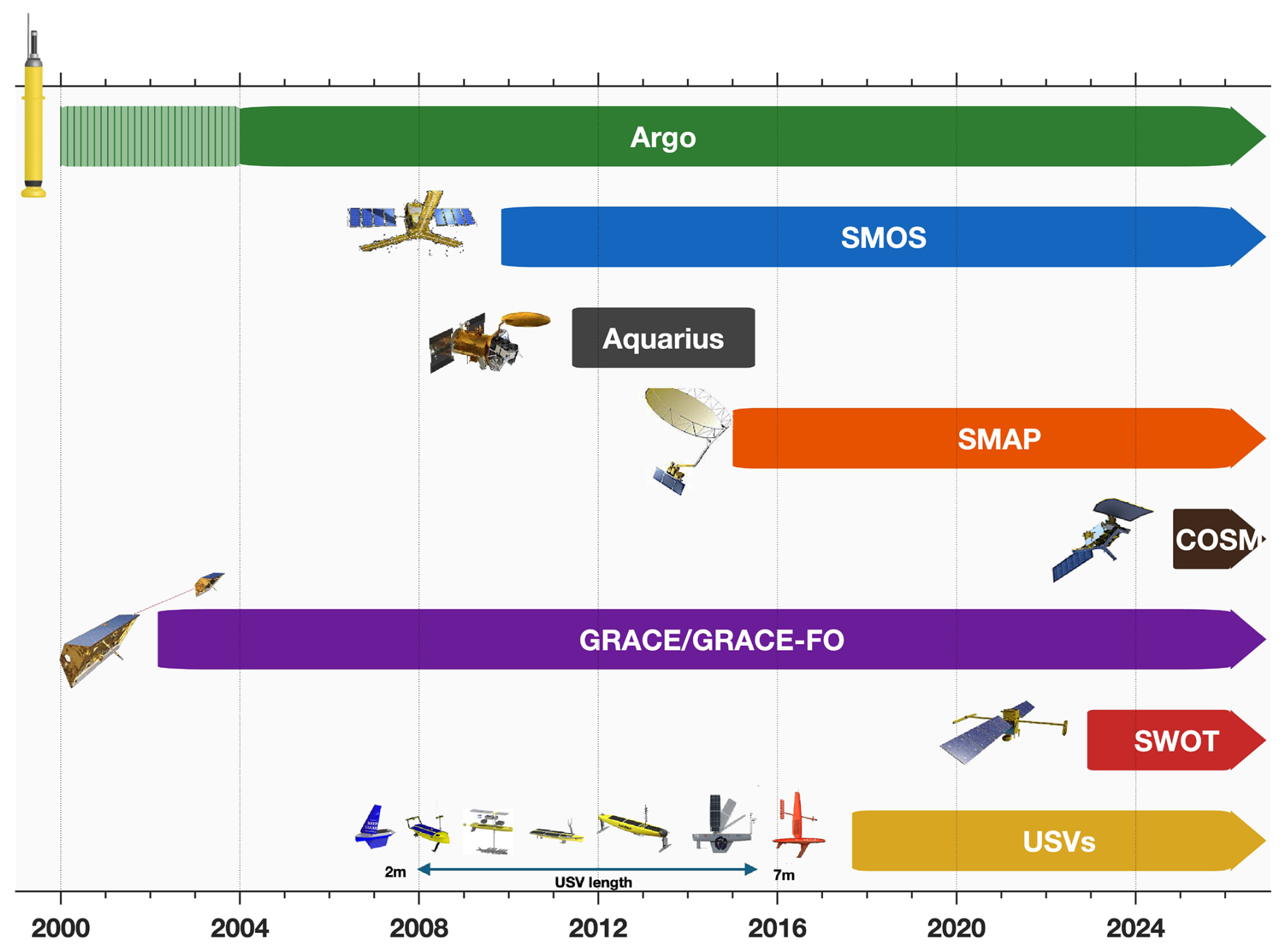
Figure 2 Timeline of major ocean observing systems for water cycle research (2000–2025). The Argo profiling float array (hatched: pilot phase 2000–2004; solid: near-global coverage 2004–present) provides continuous subsurface temperature and salinity measurements to 2000 m depth. Satellite missions SMOS (2009–present), Aquarius (2011–2015), SMAP (2015–present), and COSM (2024–present) measure sea surface salinity from L-band radiometry at ∼ 40–60 km resolution. GRACE/GRACE-FO (2002–present) constrains basin-integrated ocean mass changes that reflect $E-P-R$ (evaporation minus precipitation minus runoff) net fluxes. SWOT (2022–present) observes sea surface height at submesoscale (∼ 15 km) resolution and monitors terrestrial surface water storage and river discharge. Uncrewed surface vehicles (USVs; 2017–present) capture submesoscale (1–10 km) surface variability in temperature and salinity. These complementary systems span spatial scales from submesoscale to basin and enable integrated characterization of ocean salinity variability and water cycle fluxes. Mission images courtesy of NASA/ESA/NOAA; USVs image from Patterson et al. (2025).

Three observational advances since 2000 have enabled this integration (Fig. 2). The Argo array provides quasi-synoptic three-dimensional sampling of the upper 2000 m with approximately 3° spacing and 10 d repeat cycles (Roemmich and Gilson, 2009; Riser et al., 2016). Satellite L-band radiometry missions (SMOS, Aquarius, SMAP, COSM) deliver continuous surface salinity fields at approximately 100 km spatial and weekly temporal resolution (Boutin et al., 2018; Vinogradova et al., 2019; Reul et al., 2020). Autonomous surface vehicles and gliders resolve submesoscale variability through intensive targeted deployments achieving kilometer spatial and hourly temporal sampling (Patterson et al., 2025). GRACE/GRACE-FO and SWOT provide basin-integrated ocean mass variations and terrestrial water storage changes that constrain regional freshwater budgets (Tapley et al., 2004; Morrow et al., 2019; Vinogradova et al., 2025).

These systems address distinct observational requirements across scale regimes. Argo vertical profiles distinguish atmospheric forcing from ocean circulation. Forcing-driven anomalies remain confined to the mixed layer, while circulation-driven anomalies extend along isopycnals or track subsurface density structure. Isopycnal analysis isolates water-mass changes from vertical displacement of the density field (Bindoff and McDougall, 1994), enabling attribution of surface salinity trends to water cycle changes rather than circulation shifts (Qu et al., 2016; Zika et al., 2018). Satellite L-band radiometers (SMOS, Aquarius, SMAP) resolve the horizontal spatial coherence that sparse in situ profiling cannot capture, revealing mesoscale fronts, eddy-driven stirring, and major river plumes as organized circulation features rather than isolated point anomalies (Grodsky et al., 2012; Lee et al., 2012; Reul et al., 2014; Yu, 2015; Fournier et al., 2016, 2017; Melnichenko et al., 2017). Combined with altimetric geostrophic currents, satellite-derived winds, and E−P fields, satellite SSS enables regional freshwater budgets that partition surface salinity tendencies into local atmospheric forcing versus remote ocean advection (Vinogradova and Ponte, 2013; Dong et al., 2014; Yu, 2023). Autonomous platforms capture submesoscale features at their native scales, including rainfall-generated fresh lenses, sharp frontal salinity gradients, and barrier layers evolving at kilometers and hours (Drushka et al., 2019). Glider profiling and SWOT sea surface height observations reveal whether submesoscale salinity features remain surface-trapped or couple vertically to interior dynamics (Morrow et al., 2019; du Plessis et al., 2022).

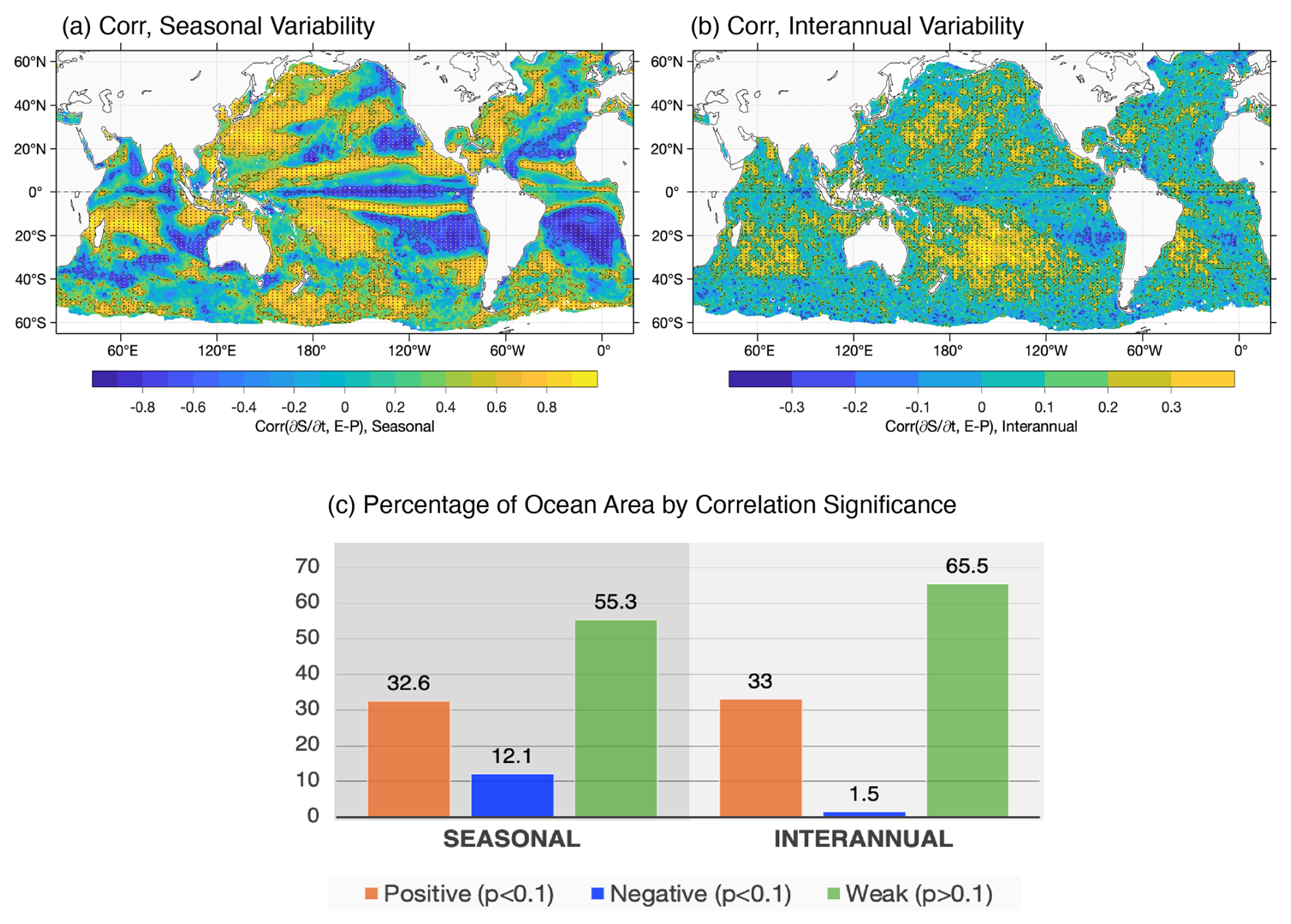
Figure 3 Correlation between E−P and $\partial S/\partial$t at seasonal and interannual timescales (2012–2022). Spatial distribution of correlation coefficients for (a) seasonal variability (demeaned) and (b) interannual variability (detrended and deseasonalized). Stippling indicates regions where correlations are statistically significant (p < 0.1). (c) Percentage of ocean area showing statistically significant positive (p < 0.1, orange), significant negative (p < 0.1, blue), and weak non-significant (p > 0.1, green) correlations. Significant positive correlations occupy 33 % of ocean area at both timescales; weak correlations dominate (55 % seasonal, 66 % interannual). Correlation thresholds for significance (p < 0.1) are 0.50 for seasonal and 0.14 for interannual variability, the latter reflecting limited degrees of freedom in the 11-year analysis period. E from OAFlux monthly 0.25° analysis (Yu, 2019), P from GPCP Monthly 0.5° v3.2 (Huffman et al., 2023), mixed layer depth h from the Argo monthly 1° gridded product (Roemmich and Gilson, 2009), and SSS from OISSS monthly 0.25° product (Melnichenko, 2023), all interpolated to a common 0.25° grid. Adapted from Yu (2023).

Observational coverage remains fundamentally asymmetric across scale regimes. Basin-scale salinity patterns and multi-decadal trends are well constrained by Argo subsurface sampling and satellite surface coverage combined, enabling robust detection of pattern amplification and separation of externally forced trends from internal climate variability. Mesoscale surface salinity structure benefits from satellite spatial continuity but lacks corresponding subsurface resolution; reconstructing three-dimensional circulation pathways and quantifying subduction rates requires vertical sampling substantially denser than Argo's nominal 3° spacing. Submesoscale salinity features evolving at kilometer spatial scales and synoptic temporal scales are systematically undersampled by all sustained observing systems, captured only during intensive field campaigns with autonomous platforms. It is also worth noting that Argo sampling is generally limited to 60° S–65° N, with sparse coverage in the Arctic Ocean and in areas with seasonal ice cover. Because the mixed layer depth h derived from Argo is a key variable in computing the freshwater forcing term FWF = $S_{\mathrm{0}}(E-P)/h$ (see Eq. 1), the analyses presented in Sect. 3 are necessarily confined to regions where Argo provides sufficient coverage to estimate h reliably; the Arctic Ocean is therefore excluded. This observational asymmetry reflects fundamental technological and resource constraints rather than design limitations: simultaneous achievement of global basin coverage, mesoscale spatial resolution, and submesoscale temporal resolution exceeds current observing system capacity. Section 3 examines salinity behavior across these observationally defined regimes.

3 Where salinity indicates water-cycle changes: timescale-dependent forcing control

Salinity acts as a water-cycle indicator when ocean processes integrate freshwater forcing faster than they redistribute it. The governing equation for mixed-layer salinity evolution is:

$$\begin{array}{}\text{(1)}& \begin{array}{r}{\displaystyle \frac{\partial S}{\partial t}}=\underset{\text{horizontal\hspace{0.17em}\hspace{0.17em}advection}}{\underbrace{-{\mathit{u}}_{\mathrm{h}}\cdot \left({\mathrm{\nabla }}_{\mathrm{h}}S\right)}}\underset{\text{vertical\hspace{0.17em}\hspace{0.17em}advection}}{\underbrace{-w{\displaystyle \frac{\partial S}{\partial z}}}}+\underset{\text{horizontal\hspace{0.17em}\hspace{0.17em}mixing}}{\underbrace{{\mathrm{\nabla }}_{\mathrm{h}}\cdot \left(K_{\mathrm{h}}{\mathrm{\nabla }}_{\mathrm{h}}S\right)}}\\ +\underset{\text{vertical\hspace{0.17em}\hspace{0.17em}mixing}}{\underbrace{{\displaystyle \frac{\partial }{\partial z}}\left(K_{\mathrm{v}}{\displaystyle \frac{\partial S}{\partial z}}\right)}}+\underset{\text{surface\hspace{0.17em}\hspace{0.17em}freshwater\hspace{0.17em}\hspace{0.17em}forcing\hspace{0.17em}\hspace{0.17em}(FWF)}}{\underbrace{{\displaystyle \frac{S_{\mathrm{0}}}{h}}(E-P-R)}}\end{array}\end{array}$$

where u_h and w are horizontal and vertical velocities, K_h and K_v are mixing coefficients, and $S_{\mathrm{0}}/h(E-P-R)$ denotes the effect of evaporation (E), precipitation (P), and runoff (R) on mixed-layer salinity. The terms on the right-hand-side represent horizontal advection, vertical advection, horizontal mixing, vertical mixing, and surface freshwater forcing (FWF), respectively. The rain gauge approximation emerges when advection and mixing terms become small relative to forcing, reducing Eq. (1) to $\partial S/\partial t\approx S_{\mathrm{0}}/h(E-P-R)$. Whether this holds depends critically on timescale: at what temporal scales does forcing accumulate faster than circulation redistributes it? Figure 3 addresses this question at seasonal and interannual timescales by correlating observed $\partial S/\partial t$ with E−P at each ocean location, showing forcing controls salinity tendency across approximately 30 % of ocean area.

3.1  Seasonal-interannual forcing dominance

Before examining the spatial patterns, it is useful to clarify how variability is defined at each timescale. Seasonal variability is isolated by removing the time-mean from monthly fields (demeaned). Interannual variability refers to year-to-year variations on timescales of 1–7 years, obtained by removing both the long-term trend and mean seasonal cycle from monthly-mean fields (detrended and deseasonalized). Figure 3 shows where forcing controls salinity variability versus where ocean circulation redistributes it. Forcing-dominated regions exhibit statistically significant positive correlations (r > 0.50 seasonal, r > 0.14 interannual; p < 0.1) between salinity tendency and local E−P. Circulation-dominated regions show weak, non-significant correlations (p > 0.1), indicating advection and mixing redistribute freshwater before forcing signatures accumulate. Significant negative correlations (r < −0.50 seasonal, r < −0.14 interannual; p < 0.1) occur where circulation processes oppose surface forcing. With an 11-year record (2012–2022), the degrees of freedom for interannual statistics are limited, and the significance threshold of r > 0.14 (p < 0.1) reflects this. The broad spatial patterns of interannual correlation are nonetheless consistent with results from longer records (Vinogradova and Ponte, 2017; Yu, 2023), supporting the robustness of the patterns shown.

Forcing-dominated regions (33 % of ocean area) concentrate in subtropical gyre interiors (20–40° N/S), semi-enclosed seas, and monsoon regions. Subtropical gyres maintain strong correlations (r = 0.6–0.7) at seasonal timescales and moderate correlations (r = 0.3–0.5) at interannual timescales, where weak advection (1–3 cm s⁻¹) (Yu, 2023) allows E−P signals to accumulate. Semi-enclosed seas exhibit strongest forcing control (r > 0.7 seasonal) because geometric constraints limit advective escape. Mediterranean evaporation (∼ 10 cm month⁻¹; Fig. 1b) creates 0.3–0.5 psu seasonal amplitude correlating at r = 0.85 with E−P (Skliris et al., 2018). Monsoon regions show timescale-dependent behavior: Bay of Bengal exhibits strong seasonal correlation (r  = 0.5–0.7) but weak interannual correlation (not significant). Monsoon precipitation (∼ 22 cm month⁻¹ during June–September; Rao and Sivakumar, 2003) creates 2–4 psu freshening on 3-month timescales shorter than lateral spreading timescales (6–9 months), enabling local accumulation. At interannual timescales, ENSO-driven current anomalies introduce variance comparable to precipitation anomalies, degrading correlation (Delcroix and Hénin, 1991; Hasson et al., 2014).

Circulation-dominated regions (55 %–66 %) include western boundary currents, equatorial upwelling zones, and subpolar gyres. Western boundary currents exhibit weak correlation because strong advection redistributes freshwater faster than forcing accumulates (Hogg and Johns, 1995). Correlation degrades from subtropical gyre interiors toward western boundaries where Gulf Stream and Kuroshio advection dominates. Equatorial upwelling zones exhibit significant negative correlation (r = −0.4 to −0.6 seasonal; 5 %–10 % of ocean area) where upwelling brings high-salinity subsurface water to the surface during precipitation seasons, notably in eastern equatorial Pacific (Maes et al., 2014). Subpolar gyres and Southern Ocean show weak correlation despite large precipitation because strong currents, deep winter mixing (200–800 m) (de Boyer Montégut et al., 2004), and energetic mesoscale eddies redistribute freshwater (Müller et al., 2019) before forcing signatures accumulate.

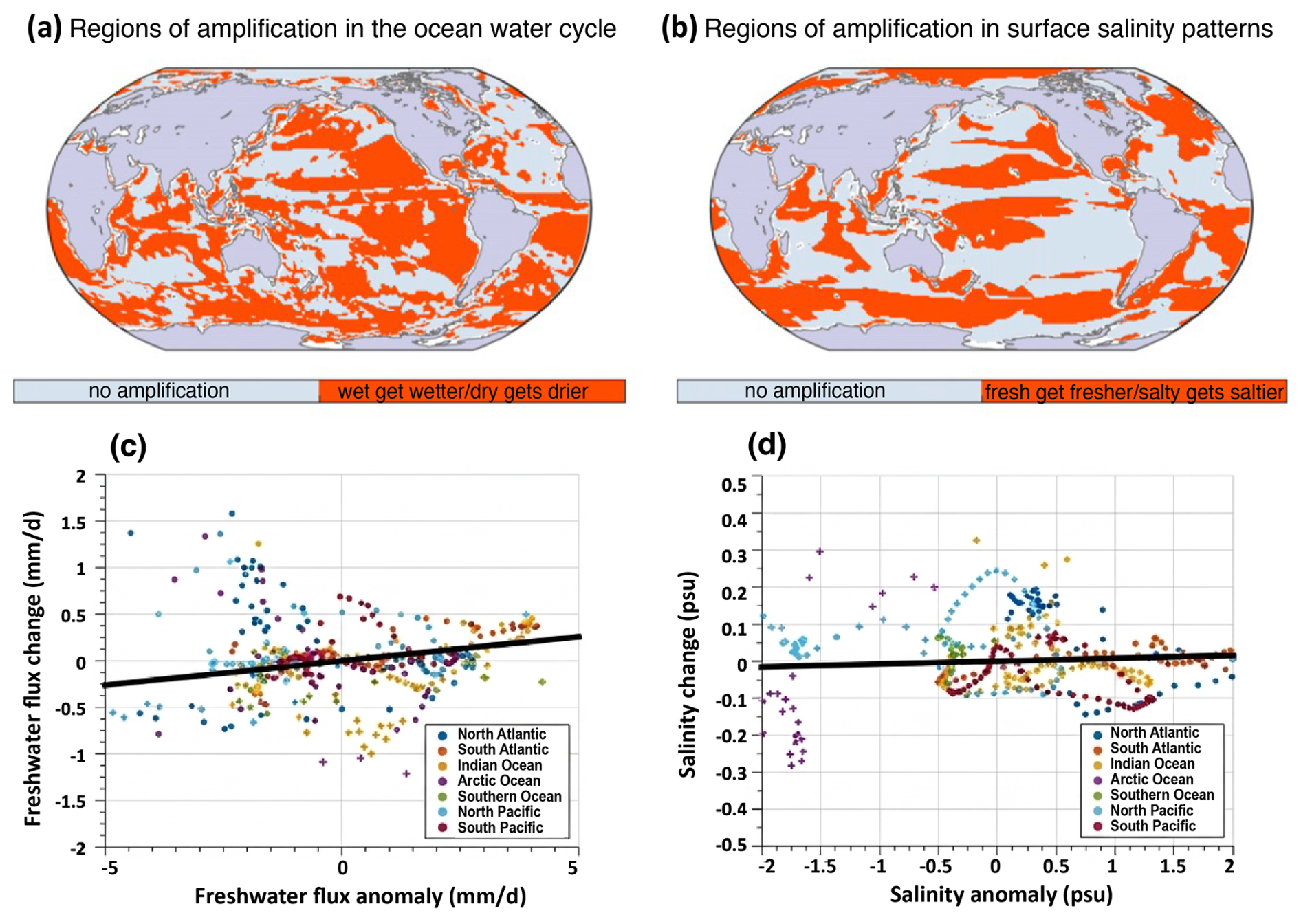
Figure 4 Pattern amplification in ocean water cycle versus surface salinity over 1993–2010. (a, b) Regions where climatological patterns amplified (orange: wet regions got wetter and dry regions got drier for freshwater flux; fresh regions got fresher and salty regions got saltier for salinity) versus weakened (gray). (c, d) Strength of pattern amplification: x-axis shows anomalies (relative to global average) in zonal ocean basin averages of climatological mean freshwater flux (c) or surface salinity (d); y-axis shows corresponding 1993–2010 changes. Colors denote ocean basins. Black line shows linear regression; slope gives total pattern amplification. Ocean water cycle amplified by 5 % globally (c), but surface salinity patterns amplified by less than 1 % globally (d). Adapted from Vinogradova and Ponte (2017).

3.2 Weak salinity pattern amplification at decadal timescales

Natural decadal variability operates on timescales comparable to 10–30 year analysis periods, complicating the detection of forced salinity signals. Decadal-scale trends reveal contrasting behavior between atmospheric forcing and ocean salinity response. Analysis of 1993–2010 shows the ocean water cycle (E−P) pattern amplified by approximately 5 %, with spatial correlation r≈ 0.5 between climatological E−P and observed trends (Vinogradova and Ponte, 2017), matching Clausius–Clapeyron expectations for atmospheric moisture response to warming (Held and Soden, 2006). Surface salinity patterns, however, amplified by less than 1 % globally, with near-zero spatial correlation between climatological patterns and observed trends (Fig. 4). Ocean basins show scattered responses: some amplify climatological patterns while others reverse them. This weak salinity pattern amplification, despite coherent atmospheric forcing, indicates that ocean processes operating on decadal timescales prevent surface salinity from tracking atmospheric forcing coherently.

Regional analysis reveals the physical basis for weak global pattern amplification. Pacific basin-average salinity decreased over 1970–2002, exceeding internal variability estimates and showing detectable anthropogenic influence, while Atlantic basin-average trends remained within internal variability range (Terray et al., 2012). This basin-scale contrast reflects differences in how circulation and natural variability compete with forcing accumulation. North Atlantic salinity over 1993–2012 exhibits large multiyear variability driven by NAO modulation of the North Atlantic Current, with circulation-driven anomalies dominating over surface freshwater forcing (Stendardo et al., 2016). Strong western boundary currents and active decadal modes redistribute North Atlantic freshwater on timescales comparable to 10–20 year forcing accumulation. The Pacific shows clearer forced trends during 2005–2015 (basin-average 2.2 × 10⁻³ psu yr⁻¹) following earlier freshening in 1994–2005 (Li et al., 2020), suggesting forced signals can emerge where circulation redistribution operates more slowly.

Salinity budgets quantify the circulation-forcing competition. Pacific upper 200 m analysis for 2005–2015 shows surface freshwater flux and ocean advection produce opposite effects, each with magnitudes approximately twice the net salinity tendency (Li et al., 2020). This opposing relationship indicates active redistribution rather than passive forcing integration. Where precipitation dominates, advection exports excess freshwater; where evaporation dominates, advection imports freshwater from elsewhere. Horizontal advection and diffusion control subtropical redistribution while vertical diffusion and entrainment control tropical and high-latitude redistribution (Lyu et al., 2025), creating regionally varying pathways that prevent globally coherent response to coherent forcing. Despite these complications, salinity exhibits higher signal-to-noise ratios than atmospheric variables such as precipitation or E−P, because salinity integrates high-variance atmospheric forcing over time while spreading anomalies spatially. As a result, detecting anthropogenic influence in SSS requires fewer than three ensemble members for SSS versus substantially more for precipitation or E−P (Terray et al., 2012).

The Interdecadal Pacific Oscillation shift from positive to negative phase around 1998–1999 contributes approximately 30 % of Pacific salinity variance, exceeding 60 % in equatorial regions (Vinogradova and Ponte, 2017). NAO variability similarly drives North Atlantic salinity through circulation changes independent of local forcing (Stendardo et al., 2016). At decadal timescales, forcing accumulation, circulation redistribution, and natural variability all operate on comparable timescales, preventing any single process from dominating. The result is coherent atmospheric forcing (+5 % pattern amplification) producing weak salinity response (< 1 % pattern amplification), showing that 10–30 year periods are insufficient for forcing signals to overwhelm circulation redistribution and natural variability. Basin differences arise where local conditions favor one process. Pacific shows partial forcing dominance where redistribution is slower, Atlantic shows variability dominance where energetic currents operate faster. Longer integration periods are required for forcing to accumulate decisively beyond redistribution timescales, as examined in Sect. 3.3 for multi-decadal scales.

3.3 Multi-decadal pattern emergence

Over multi-decadal timescales (50+ years), the influence of freshwater forcing on ocean salinity becomes clearly detectable, although these patterns remain obscure at shorter timescales (Figs. 3 and 4). Spatial correlation between 1950–2000 salinity trends and climatological SSS patterns reaches r = 0.7–0.8, indicating fresh regions systematically freshened while salty regions salinified over 50+ year periods (Durack and Wijffels, 2010; Durack et al., 2012). This pattern correlation contrasts sharply with near-zero values at decadal timescales (Fig. 4b and d), showing that forcing accumulation over 50+ years produces spatially coherent salinity response despite circulation redistribution. The 145-year record of ocean salinity measurements, obtained from HMS Challenger and SMS Gazelle expeditions (1870s) through modern observations, demonstrates that pattern amplification has been detectable since the early industrial era, but with marked acceleration. Rates increased from ∼ 0.166 $\mathrm{g}{\mathrm{kg}}^{-\mathrm{1}}{\mathrm{century}}^{-\mathrm{1}}$ (1870s–1950s) to ∼ 0.306 $\mathrm{g}{\mathrm{kg}}^{-\mathrm{1}}{\mathrm{century}}^{-\mathrm{1}}$ (1950s–2010s), a 54 ± 10 % acceleration (Gould and Cunningham, 2021). Spatial correlation between regional salinity changes across these periods (r=0.64) indicates persistent forcing-driven patterns since the 1870s, though with non-linear intensification. Recent decades show further acceleration, with post-1991 rates nearly doubling those of 1960–1990 (Cheng et al., 2020; Douville and Cheng, 2024).

Regional patterns of E−P show quantitatively consistent amplification across independent analyses at 4 % °C⁻¹–8 % °C⁻¹ (Durack and Wijffels, 2010; Helm et al., 2010; Skliris et al., 2016), in line with Clausius–Clapeyron predictions for atmospheric moisture response to warming (Held and Soden, 2006). Tropical and subpolar fresh regions (climatological P > E) freshened 0.2–0.4 psu over 1950–2000, while subtropical salinity maxima (climatological E > P regions) increased 0.1–0.3 psu (Curry et al., 2003; Durack and Wijffels, 2010). However, pattern amplification exhibits marked asymmetry: freshening in low-salinity regions proves far more robust across ocean basins with consistent spatial patterns and strong emergence from natural variability, whereas salinification in subtropical gyres displays greater sensitivity to region definition and weaker signal-to-noise ratios (Cheng et al., 2020; Douville and Cheng, 2024). The Mediterranean Sea and Baltic Sea provide particularly clear evidence where geometric constraints can enhance forcing signals. In the Mediterranean, salinification (0.10–0.15 psu) has been linked to 10 %–15 % evaporation increases (Skliris et al., 2018), while in the Baltic, freshening (0.10–0.20 psu) is consistent with increased precipitation and runoff (Meier et al., 2006; Lehmann et al., 2022).

Attribution studies identify the different physical processes driving the observed pattern amplification. Observed multi-decadal patterns have less than 5 % probability of arising from internal variability alone when major climate modes are removed, with approximately two-thirds of variance attributable to external forcing (Pierce et al., 2012; Terray et al., 2012). CMIP5 simulations show the emergence of anthropogenic influence. Historical runs incorporating all forcings reproduce observed spatial patterns and amplification magnitude, whereas natural-forcing-only simulations show no significant trends (Cheng et al., 2020). Mechanistic decomposition using ocean model experiments reveals three contributing processes (Zika et al., 2018): direct surface freshwater flux changes from water cycle intensification, ice mass loss contributions (relatively minor), and ocean warming effects on stratification. Ocean warming proves particularly important because warming-induced stratification inhibits vertical mixing, effectively preserving and amplifying surface salinity patterns. Warming explains approximately half of surface salinity pattern changes from 1957–2016, with water cycle intensification of 3.6 % °C⁻¹ ± 2.1 % °C⁻¹ accounting for the remainder. These changes exceed 2σ natural variability (> 95 % confidence) (Zika et al., 2018), showing human influence on ocean salinity patterns since 1960 (Pierce et al., 2012; Terray et al., 2012).

Table 1 Fundamental timescales governing salinity evolution.

The physical mechanisms enabling multi-decadal pattern emergence operate through timescale separation and stratification enhancement rather than circulation suppression. Surface E−P anomalies create near-surface salinity changes that subsequently subduct along isopycnals into low-latitude subsurface layers via subtropical gyre ventilation (Durack et al., 2012), advect poleward and downward through intermediate water formation driving broad 300–2000 m freshening (Helm et al., 2010), and interact with ocean warming to enhance high-latitude stratification and reduce vertical mixing that would otherwise erode surface salinity contrasts (Zika et al., 2018). At multi-decadal scales, circulation contributions remain important (Jarugula et al., 2025). The Atlantic-Pacific salinity contrast increased 5.9 ± 0.6 % over 1965–2020, yet direct $E-P-R$ forcing explains less than half this change, with the remainder from circulation adjustments including thermocline heaving, cross-basin moisture transport, and gyre intensification (Singh et al., 2016; Friedman et al., 2017; Zika et al., 2021; Lu et al., 2024). What distinguishes multi-decadal from shorter timescales is not that circulation stops, but that forcing accumulates over 50+ years while basin-scale redistribution operates on 5–20 year timescales. Because forcing persists much longer than redistribution and mixing processes, it can build up a coherent signal despite ongoing circulation. Forcing controls only 30 % of ocean area at seasonal-interannual scales (Fig. 3) and produces less than 1 % pattern amplification at decadal scales (Fig. 4), but generates strong pattern correlations (r = 0.7–0.8) and 54 % acceleration post-1950s at multi-decadal scales. This progression shows that forcing fingerprints emerge when forcing timescales far exceed redistribution timescales, consistent with the rain gauge paradigm over sufficiently long periods and revealing ocean warming as a critical amplifying mechanism.

4 When circulation controls salinity: timescale competition and regime transitions

Section 3 documented a striking timescale dependence in how salinity responds to freshwater forcing. Forcing controls salinity tendency across ∼ 30 % of ocean area at seasonal-interannual timescales (Fig. 3), yet produces < 1 % pattern amplification at decadal scales despite 5 % atmospheric forcing amplification (Fig. 4). At multi-decadal scales, however, forcing fingerprints emerge with strong spatial pattern correlations (r = 0.7–0.8). What physical mechanisms explain these regime transitions?

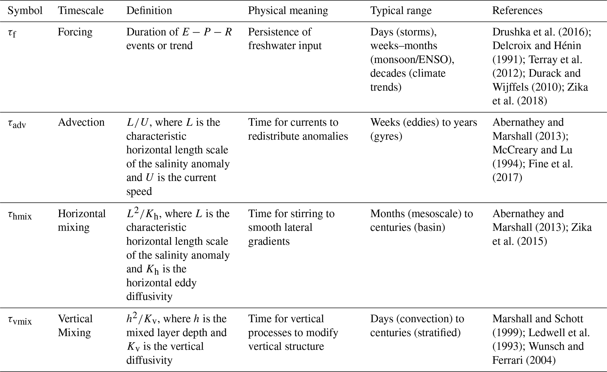
The question is not whether forcing or circulation “controls” salinity, since both always operate. Rather, we ask: Does the spatial distribution of salinity anomalies match the spatial distribution of forcing, or does it trace the pathways by which circulation redistributes remotely forced anomalies? The answer lies in competition among four characteristic timescales governing Eq. (1). Table 1 defines these timescales: the forcing timescale τ_f measures how fast freshwater fluxes change, the advection timescale ${\mathit{\tau }}_{\text{adv}}=L/U$ measures how fast currents redistribute anomalies, the horizontal mixing timescale ${\mathit{\tau }}_{\text{hmix}}=L^{\mathrm{2}}/K_{\mathrm{h}}$ measures how fast stirring erodes gradients, and the vertical mixing timescale ${\mathit{\tau }}_{\text{vmix}}=h^{\mathrm{2}}/K_{\mathrm{v}}$ measures how fast vertical processes modify stratification.

Three primary competitions emerge from these timescales. First, τ_f versus τ_adv determines whether forcing accumulates coherently (rain gauge) or anomalies transport far from formation regions (passive tracer). Second, τ_vmix versus τ_adv controls whether subsurface waters preserve formation-era memory or respond to contemporary forcing. Third, convergence of all four timescales at submesoscales creates a dynamical regime where salinity actively shapes density structure. The horizontal mixing timescale τ_hmix (decades to centuries for basin scales) is typically much longer than τ_f, τ_adv, and τ_vmix, so while it determines whether anomalies maintain coherence during transport, it rarely competes directly except at submesoscales where all timescales converge.

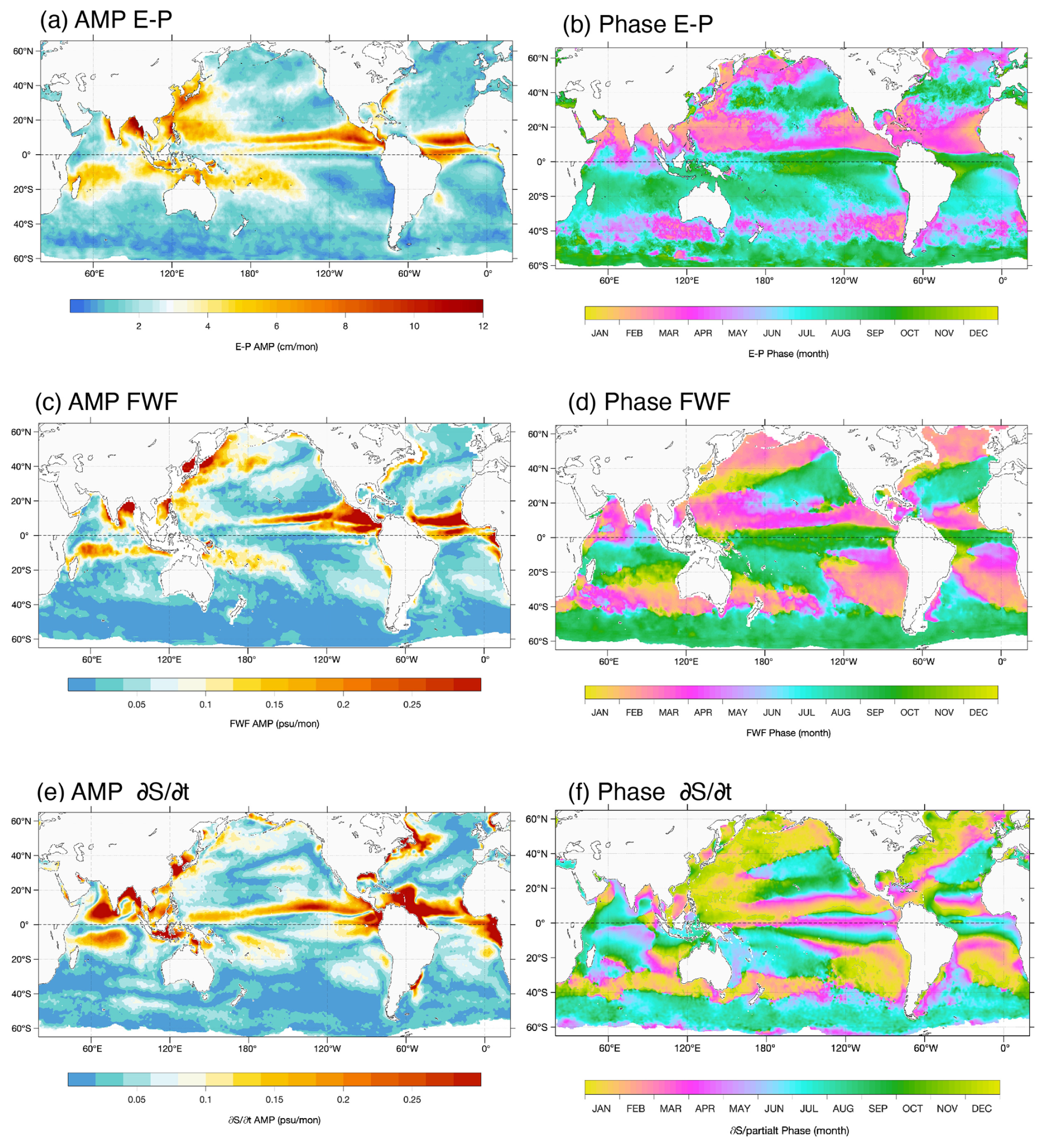
Figure 5 Amplitude-phase asymmetry in seasonal salinity variability demonstrates forcing sets variance amplitude but circulation determines spatial-temporal distribution. Harmonic analysis of (a, b) atmospheric freshwater forcing E−P, (c, d) freshwater flux FWF = $S_{\mathrm{0}}(E-P)/h$, and (e, f) observed salinity tendency $\partial S/\partial t$ from satellites (2010–2020). Left panels show seasonal amplitude; right panels show phase (month of annual maximum). E is from OAFlux monthly 0.25° analysis (Yu, 2019), P from GPCP Monthly 0.5° v3.2 (Huffman et al., 2023), mixed layer depth h from the Argo monthly 1° gridded product (Roemmich and Gilson, 2009), and SSS from OISSS monthly 0.25° product (Melnichenko, 2023). All datasets are interpolated to a common 0.25° grid. Salinity tendency $\partial S/\partial t$ in panels (e, f) is computed as the temporal derivative of monthly-mean SSS, and harmonic analysis is then applied to all monthly-mean fields. Adapted from Yu (2023).

4.1 Amplitude-phase separation and horizontal pathways

4.1.1 Amplitudes agree, phases differ

Figure 5 reveals a fundamental separation in how salinity responds to freshwater forcing. Seasonal amplitude patterns are strikingly coherent across atmospheric forcing E−P (Fig. 5a), mixed-layer forcing FWF = $S_{\mathrm{o}}(E-P)/h$ (Fig. 5c), and observed salinity tendency $\partial S/\partial t$ (Fig. 5e), with amplitudes exceeding 0.2 psu per month in tropical convergence zones and 0,1 psu per month in subtropical net evaporation maxima. This amplitude coherence indicates that forcing magnitude controls salinity variance.

However, phase maps tell a different story. Across most ocean regions, $\partial S/\partial t$ phase (Fig. 5f) leads E−P phase (Fig. 5b) by 1–3 months. The eastern tropical Pacific exemplifies this behavior. Local E−P reaches maximum in March-April when the ITCZ migrates southward (Fig. 5b), yet $\partial S/\partial t$ peaks earlier in January-March. Similarly, $\partial S/\partial t$ in the subtropical North Pacific leads E−P by approximately 2 months. This phase lead is stronger evidence for circulation control than a lag would be. A phase lag might indicate slow local response to forcing, but a phase lead requires non-local processes. Salinity cannot respond to local forcing before that forcing occurs. The phase lead indicates that salinity changes reflect ocean processes, either through advection of anomalies from upstream regions where forcing peaked earlier in the seasonal cycle, or upwelling of subsurface water with different seasonal history, or remote forcing effects transported by circulation. Forcing creates the variance, but circulation determines when and where that variance manifests.

The progressive phase shift from $E-P\to \mathrm{FWF}\to \partial S/\partial t$ in Fig. 5b, d, and f quantifies how ocean processes successively alter salinity timing. The E−P to FWF phase shift reflects mixed-layer depth modulation, where deeper winter mixed layers dilute the same freshwater flux over larger volumes. The FWF to $\partial S/\partial t$ phase shift isolates pure circulation effects operating through horizontal advection, vertical exchanges, and mixing. Subtropical gyre interiors where all three phases align represent forcing-dominated regimes. Upwelling zones, boundary currents, and monsoon regions showing large phase differences between FWF and $\partial S/\partial t$ represent circulation-dominated regimes where advection competes directly with forcing accumulation.

4.1.2 Multi-decadal versus seasonal regimes

The timescale framework from Table 1 explains why forcing control strengthens from seasonal to multi-decadal timescales. At seasonal-interannual timescales, τ_f (seasonal forcing persistence, ∼ 3–12 months; ENSO, ∼ 2–5 years) proves comparable to τ_adv for surface redistribution (mesoscale eddies, ∼ weeks to months; gyre-scale transport, ∼ months to years). When ${\mathit{\tau }}_{\mathrm{f}}/{\mathit{\tau }}_{\text{adv}}\mathrm{1}$, forcing creates variance but advection redistributes it before coherent spatial patterns emerge. Figure 3 shows this regime where temporal correlation between $\partial S/\partial t$ and E−P remains weak (< 0.4) across 70 % of ocean area. The forcing signal exists but advection scrambles it spatially and temporally, as shown by the phase differences in Fig. 5.

At multi-decadal timescales, the ratio shifts. Forcing accumulates over τ_f ∼ 50–100 years while basin-scale redistribution through gyre circulation, subtropical cells, and meridional overturning operates on τ_adv ∼ 5–20 years (McCreary and Lu, 1994; Gu and Philander, 1997; Qu et al., 2013; Fine et al., 2017). This gives ${\mathit{\tau }}_{\mathrm{f}}/{\mathit{\tau }}_{\text{adv}}\approx$ 5–10. When forcing persists much longer than redistribution timescales, circulation repeatedly samples the same forcing pattern. Subtropical gyre water recirculates within the high-evaporation subtropical band every 5–10 years, experiencing persistent E > P forcing with each circulation cycle. Over 50–100 years, this repeated exposure to the same forcing regime accumulates coherent basin-scale salinity trends that spatially match the forcing pattern. The spatial correlation emerges not because circulation stops redistributing anomalies, but because circulation pathways remain within forcing regimes long enough for forcing to accumulate systematically. The spatial pattern correlation between multi-decadal salinity trends and climatological E−P reaches r = 0.7–0.8 (Durack and Wijffels, 2010; Skliris et al., 2016; Cheng et al., 2020). Fresh regions systematically freshen, salty regions systematically salinify. Circulation still redistributes anomalies actively, but forcing accumulates persistently, imposing its spatial fingerprint.

Figure 4 captures the critical transition at decadal timescales (10–30 years), where ${\mathit{\tau }}_{\mathrm{f}}/{\mathit{\tau }}_{\text{adv}}\approx$ 1–2. Atmospheric forcing amplifies coherently (5 % pattern intensification) but ocean salinity responds incoherently (< 1 % pattern amplification). This asymmetric response reflects the fact that forcing and redistribution operate on comparable timescales. Basin-scale adjustment processes including gyre spinup, thermocline heaving, and ENSO-driven reorganization all operate over 5–20 years (Anderson and Gill, 1975; Lysne and Deser, 2002; Cessi and Otheguy, 2003; McPhaden et al., 2006), meaning τ_adv and τ_f are comparable at decadal scales and neither process dominates. The atmosphere intensifies its hydrological cycle, but ocean circulation redistributes anomalies as soon as forcing creates patterns.

Table 2 River plume spatial progression as analog of open-ocean timescale regimes.

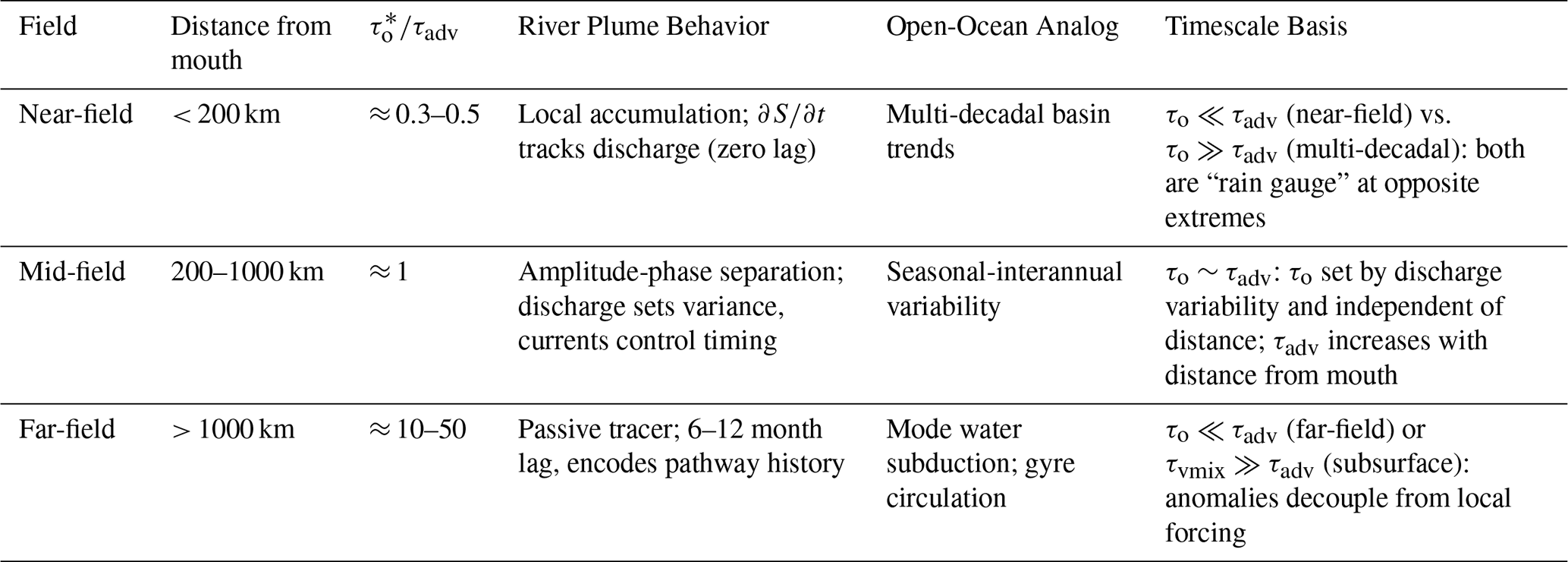
^∗ τ_o denotes the river outflow variability timescale, determined by discharge variability and ranging from days (flood events) to months (seasonal cycle) depending on the river system and the type of forcing considered. Unlike τ_adv, which increases with distance from the river mouth, τ_o is independent of distance from the mouth.

The progression from 30 % spatial control (seasonal, ${\mathit{\tau }}_{\mathrm{f}}/{\mathit{\tau }}_{\text{adv}}\mathrm{1}$) through < 1 % pattern amplification (decadal, ${\mathit{\tau }}_{\mathrm{f}}/{\mathit{\tau }}_{\text{adv}}\approx$ 1–2) to r = 0.7–0.8 pattern correlation (multi-decadal, ${\mathit{\tau }}_{\mathrm{f}}/{\mathit{\tau }}_{\text{adv}}\approx$ 5–10) quantifies how the ratio ${\mathit{\tau }}_{\mathrm{f}}/{\mathit{\tau }}_{\text{adv}}$ controls whether forcing or circulation dominates salinity evolution. The ocean-atmosphere system operates identically at all timescales, but forcing accumulation becomes progressively more effective at longer integration periods because circulation can only redistribute anomalies over finite timescales while forcing persists continuously.

4.1.3 River plumes as extreme cases

River plumes illustrate the full spectrum of ${\mathit{\tau }}_{\mathrm{o}}/{\mathit{\tau }}_{\text{adv}}$ regimes within a single system and clarify how the “amplitudes agree, phases differ” behavior in Sect. 4.1.1 emerges from the competition between local forcing and redistribution. In the river plume context, the relevant forcing timescale is the river outflow variability timescale, denoted τ_o to distinguish it from the atmospheric freshwater fluxes (E−P) timescale τ_f used in previous sections. For large systems such as the Amazon, τ_o can range from days (individual flood events) to months (seasonal discharge cycle), while plume evolution spans from near-field accumulation (days) through mid-field redistribution (weeks) to far-field dispersal (months to years) (Grodsky et al., 2014; Horner-Devine et al., 2015; Reul et al., 2014; Fournier et al., 2023; Olivier et al., 2024). Unlike τ_adv, which increases with distance from the mouth as currents take progressively longer to redistribute anomalies, τ_o is determined by the river and is independent of distance. So a single plume spans ${\mathit{\tau }}_{\mathrm{f}}/{\mathit{\tau }}_{\text{adv}}$ < 1, ≈ 1, and > 1 as an observable horizontal gradient, with the spatial extent of each regime varying depending on the discharge timescale considered. This spatial progression produces regime transitions analogous to the seasonal–multi-decadal progression in Sect. 4.1.2, but with τ_adv varying in space rather than τ_o varying in time. Table 2 compares these river plume regimes with their open-ocean analogues.

The near-field (< 200 km from river mouth) shows a forcing-dominated regime with ${\mathit{\tau }}_{\mathrm{o}}/{\mathit{\tau }}_{\text{adv}}\approx$ 0.3–0.5, where τ_o ranges from days to weeks depending on the discharge event, while boundary-current export requires weeks (τ_adv ∼ 2–3 weeks). Here redistribution is too slow to compete with local accumulation regardless of whether τ_o is days or weeks, so salinity tracks discharge with minimal phase lag (Fig. 5 – style phase alignment). To leading order, a simple volume-averaged salt balance gives $\partial S/\partial t\approx -S_{\mathrm{0}}Q/\left(hA\right)$, where Q is the river freshwater volume flux into the control region (m³ s⁻¹), A is the horizontal area over which that freshwater is distributed, and h is the effective plume thickness (so V=hA). Equivalently, defining an area-normalized runoff flux $R\equiv Q/A$ (m s⁻¹) yields $\partial S/\partial t\approx -S_{\mathrm{0}}R/h$ (Horner-Devine et al., 2015), making explicit that the tendency scales with freshwater input per unit mixed-layer volume. In this “forcing dominance by slow removal” limit, advection is present but subdominant in the tendency budget and does not set the phase, contrasting with the multi-decadal forcing dominance in Sect. 4.1.2, where forcing wins by persisting longer than redistribution.

The mid-field (200–1000 km) marks the transition where τ_o∼τ_adv. Here τ_o remains set by discharge variability as before, but τ_adv has increased with distance to the point where it is now comparable to τ_o, producing amplitude-phase separation. What changes with distance is therefore τ_adv, not τ_o. Discharge still largely sets the magnitude of salinity variance, but timing increasingly reflects redistribution by boundary currents, eddies, and rings, so salinity can retain discharge-like amplitudes while exhibiting phase shifts and reduced coherence with contemporaneous forcing (Fournier et al., 2017; Olivier et al., 2024). This mirrors Fig. 5, where forcing imprints variance, but circulation determines when that variance appears at a given location.

The far-field (> 1000 km) exhibits passive-tracer behavior with ${\mathit{\tau }}_{\mathrm{o}}/{\mathit{\tau }}_{\text{adv}}\approx$ 10–50, where τ_o, ranging from weekly to monthly discharge fluctuations, becomes fast compared to 6–12 month transit times. In this regime, present-day salinity no longer tracks contemporaneous discharge timing; it primarily encodes water-mass age, pathway, and the integrated history of earlier forcing that has been advected and mixed. The Amazon plume detected in the Caribbean ∼ 2000 km from the river mouth exemplifies this through lagged discharge–salinity relationships and ring-mediated transport (Hellweger and Gordon, 2002; Salisbury et al., 2011).

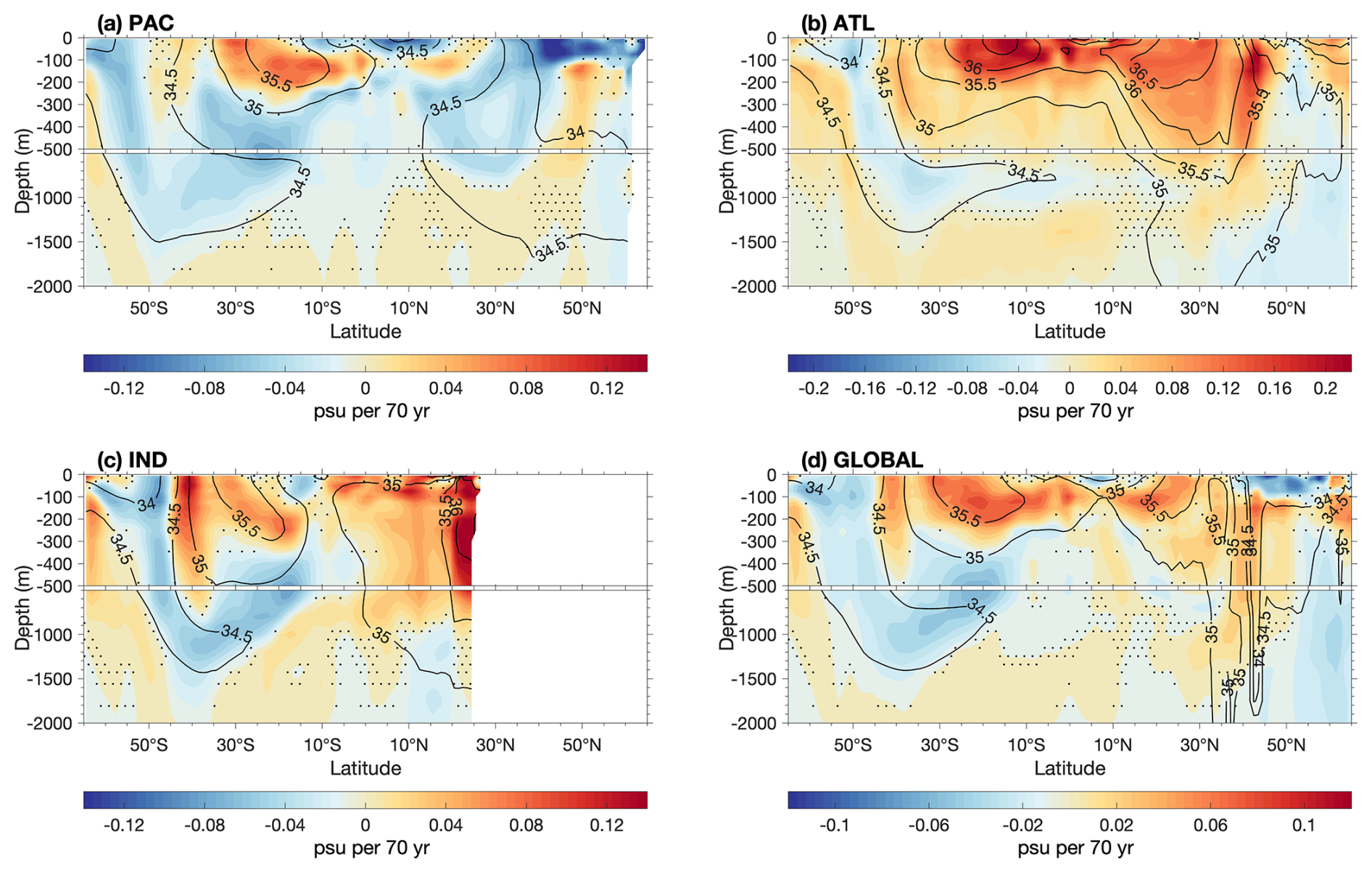
Figure 6 Subsurface salinity trends reveal circulation memory through surface-subsurface asymmetry. Zonally-averaged linear trends (1950–2019) in the upper 2000 m for (a) Pacific, (b) Atlantic, (c) Indian, and (d) global ocean. Black contours show climatological mean salinity (psu); colors show trends (psu per 70 years); stippling indicates trends not significant at 90 % confidence. y-axis scale changes at 500 m depth. In subtropical gyres (20–40° N/S), maximum trends occur at subsurface mode-water depths (100–500 m), vertically offset from surface forcing. Data from EN4 analysis (Good et al., 2013).

Pathway coherence depends on ${\mathit{\tau }}_{\mathrm{o}}/{\mathit{\tau }}_{\text{hmix}}$, where ${\mathit{\tau }}_{\text{hmix}}=L^{\mathrm{2}}/K_{\mathrm{h}}$, with L being the spatial scale of the plume (∼ 1500 km for the Amazon plume) and K_h the horizontal eddy diffusivity, determines survival against lateral stirring. For the Amazon plume extending ∼ 1500 km, τ_hmix ∼ 70 years far exceeds τ_adv ∼ 6 months, allowing coherent transport. Satellite SSS and multisensor plume mapping highlight this coherence while also showing that mesoscale stirring and ring interactions redistribute freshwater laterally without immediately erasing the large-scale signal (Reul et al., 2014; Fournier et al., 2017). Subtropical-to-tropical cells show similar persistence, where τ_adv∼ 3–5 years ≪τ_hmix ∼ centuries preserves formation signatures during equatorward transit (McCreary and Lu, 1994; Qu et al., 2013).

4.2 Surface-subsurface differences and vertical pathways

Section 4.1 examined how horizontal advection competes with forcing to create spatial and temporal patterns. The vertical dimension introduces a fundamentally different competition between vertical mixing timescale τ_vmix and horizontal advection timescale τ_adv. At the surface where τ_vmix is short (days for wind mixing, weeks for convection) (Kraus and Turner, 1967; Niiler, 1975; Marshall and Schott, 1999), salinity responds quasi-instantaneously to $E-P-R$ forcing. Below the mixed layer where stratification suppresses vertical exchange, τ_vmix increases dramatically (decades to centuries for diffusive mixing through the permanent pycnocline) (Ledwell et al., 1993; Wunsch and Ferrari, 2004), while τ_adv remains moderate (years for subtropical cells, decades for gyre circulation) (Fernandez et al., 2015). This reversal in timescale ratios creates a vertical regime boundary where salinity transitions from recording contemporary forcing to preserving formation-era conditions.

4.2.1 Surface-subsurface differences in observed trends

Figure 6 reveals systematic vertical structure in multi-decadal salinity trends that cannot be explained by local forcing. In subtropical gyres (20–40° N/S) across all ocean basins, maximum trends occur at subsurface mode-water depths (100–500 m), vertically offset from the surface where E−P forcing acts (Durack and Wijffels, 2010; Cheng et al., 2020). The Pacific (Fig. 6a) shows subsurface trend maxima of 0.08–0.1 psu per 70 years centered at 200–300 m depth near 30° N and 30° S, with negative trends present across the upper water column in the tropics with no clear surface intensification, consistent with the competing effects of freshening and subduction in this region. The Atlantic (Fig. 6b) shows strong positive trends exceeding 0.16 psu per 70 years in the South Atlantic subtropical gyre. In the 30–10° S band, the maximum trend is concentrated in the upper 100 m, with the signal of subduction manifesting as a spatial displacement of the trend maximum poleward and downward from the surface forcing region, consistent with subduction along sloping isopycnals, rather than as a simple vertical intensification below the surface. The Indian Ocean (Fig. 6c) shows a comparable vertical structure despite different surface forcing patterns.

This surface-subsurface difference indicates that observed trends reflect subduction of surface-formed anomalies along isopycnal pathways rather than in situ response to local forcing. If trends resulted from direct forcing response throughout the water column, maximum trends would occur at the surface where E−P forcing is strongest and decrease monotonically with depth as the forcing signal diffuses downward. Instead, the spatial displacement of trend maxima away from the surface forcing region indicates that surface anomalies are actively transported to depth along sloping isopycnals faster than vertical mixing can homogenize them (McCreary and Lu, 1994; Qu et al., 2013; Fine et al., 2017). The subsurface ocean thus preserves a multi-decadal memory of surface forcing history, with trend magnitude and depth distribution reflecting the integrated history of surface forcing variations and subduction pathways. It is worth noting that subduction pathways follow density surfaces rather than depth intervals, so the signal of subduction in depth coordinates naturally appears as a spatial displacement rather than a clean vertical offset. In addition, depth-coordinate representations include two distinct signals: salinity changes along isopycnals due to subduction and water-mass transformation, and apparent salinity changes due to isopycnal heaving driven by thermal expansion and density field changes over the 1950–2019 period. Separating these two contributions requires working in isopycnal coordinates, where the heaving effect can be explicitly removed (Bindoff and McDougall, 1994), An isopycnal representation would therefore more directly illustrate the subduction pathways, though converting the EAN4 product to isopycnal coordinates over the 1950–2019 period requires careful treatment of the concurrently changing density field, and is left for future work.

4.2.2 Timescale competition: τ_vmix versus τ_adv

The surface-subsurface differences arise from competing vertical mixing and horizontal advection timescales. At the surface, τ_vmix ∼ days to weeks (set by wind-driven turbulence and convective overturning) proves much shorter than τ_adv ∼ weeks to months (set by mesoscale eddies and boundary currents redistributing surface anomalies horizontally) (Niiler, 1975; Marshall and Schott, 1999; Abernathey and Marshall, 2013). This gives ${\mathit{\tau }}_{\text{vmix}}/{\mathit{\tau }}_{\text{adv}}\ll \mathrm{1}$, allowing forcing signals to mix vertically through the mixed layer before horizontal advection can redistribute them laterally.

Below the seasonal thermocline, the ratio reverses. Stratification suppresses vertical exchange, increasing τ_vmix to decades or centuries for diffusive mixing across the permanent pycnocline (Ledwell et al., 1993; Wunsch and Ferrari, 2004). Meanwhile, τ_adv for horizontal transport along isopycnals remains moderate at years to decades for subtropical cells (McCreary and Lu, 1994; Johnson and McPhaden, 1999) and decades for gyre-scale circulation (Qu et al., 2013; Fernandez et al., 2015; Fine et al., 2017). This gives ${\mathit{\tau }}_{\text{vmix}}/{\mathit{\tau }}_{\text{adv}}\gg \mathrm{1}$ in the permanent thermocline, meaning horizontal advection redistributes anomalies along density surfaces much faster than vertical mixing can erase them. Water parcels retain their formation-region salinity signatures for years to decades as they travel along isopycnal pathways, creating the subsurface “memory” visible in Fig. 6.

The regime boundary occurs where τ_vmix ∼ τ_adv, typically near the base of the winter mixed layer (50–200 m depth depending on latitude and basin). Above this depth, vertical processes dominate and salinity reflects contemporary forcing (Kraus and Turner, 1967; Niiler, 1975). Below this depth, horizontal advection along isopycnals dominates and salinity reflects formation-era conditions from years to decades earlier (McCreary and Lu, 1994; Johnson and McPhaden, 1999). The exact depth of this transition varies seasonally (deepening in winter when convection penetrates deeper) and geographically (deeper in subtropical mode water formation regions where vigorous winter convection creates thick homogeneous layers) (Hanawa and Talley, 2001; de Boyer Montégut et al., 2004).

4.2.3 Subduction and subsurface memory

Subduction physically accomplishes the τ_vmix≫τ_adv regime described in Sect. 4.2.2 through a seasonal cycle of ventilation and capping. Each winter, convection homogenizes surface waters, creating mixed layers whose salinity reflects integrated winter forcing. When spring arrives and the ocean restratifies, a seasonal thermocline reforms above these winter-formed waters, sealing them from further surface contact. These capped layers then spread horizontally along constant density surfaces into the ocean interior (Hanawa and Talley, 2001).

In the North Atlantic, high evaporation creates surface salinity maxima that subduct to form Subtropical Underwater (STUW), a subsurface salinity maximum at 100–200 m depth 20–40° N. The strong salinification trends (0.16–0.2 psu per 70 years) in this layer is visible in Fig. 6b, reflecting both intensifying surface evaporation and poleward shifts in ventilation regions (Yu et al., 2018; Liu et al., 2019). The South Pacific operates similarly through subtropical mode water formation, producing the subsurface maximum at 200–300 m in Fig. 6a. In both cases, the interior accumulates a long-term forcing signal while the surface experiences continual seasonal cycling (Marshall et al., 1993; Qiu and Huang, 1995).

The persistence timescale follows from weak vertical exchange across the permanent thermocline. With diapycnal diffusivity K_v ∼ 10⁻⁵ m² s⁻¹ and thermocline thickness h ∼ 200–300 m, vertical mixing operates on ${\mathit{\tau }}_{\text{vmix}}=h^{\mathrm{2}}/K_{\mathrm{v}}$ ∼ 50–100 years (Ledwell et al., 1993). Horizontal transport covers basin scales in τ_adv ∼ 5–10 years. The ratio ${\mathit{\tau }}_{\text{vmix}}/{\mathit{\tau }}_{\text{adv}}$ ∼ 10 means water parcels travel thousands of kilometers before vertical exchange significantly modifies their properties. The seasonal thermocline acts as a barrier, with rapid surface mixing (days) above and slow diffusion below.

This mechanism breaks down where stratification weakens. In subpolar regions, vigorous winter convection erodes the permanent thermocline, reducing the vertical barrier. Near the equator, strong upwelling and tropical instability waves enhance mixing to K_v ∼ 10⁻⁴ m² s⁻¹, reducing τ_vmix to 5–10 years. When τ_vmix ∼ τ_adv, vertical exchange modifies properties during transit. In the tropical regions, strong upwelling and enhanced mixing reduce the vertical barrier between surface and subsurface waters, so that surface freshwater anomalies are more readily communicated downward and the trend structure tends to be more uniform with depth rather than showing the clear subsurface maximum characteristic of subtropical subduction (Fig. 6a and d).

4.3 Submesoscale transition: when all timescales converge

Section 4.1 and 4.2 described regimes in which controlling timescales are cleanly ordered, so salinity behaves primarily as a recorder. When τ_f≫τ_adv, salinity integrates persistent freshwater forcing and large-scale patterns resemble the forcing patterns (rain gauge behavior). When τ_f≪τ_adv or τ_vmix≫τ_adv, salinity is exported and preserved along pathways, mapping circulation and formation histories (passive tracer behavior).

At submesoscales O(1–10 km) this ordering breaks down because the relevant processes operate on comparable hours-to-days timescales. Mixed-layer instabilities, frontogenesis, and surface forcing all evolve fast enough that no single process sets salinity before the others act (Boccaletti et al., 2007; Thomas and Ferrari, 2008; McWilliams, 2016). Salinity cannot simply integrate forcing because forcing varies on the same timescale as advection redistributes anomalies. It cannot passively inherit upstream properties because the upstream field is itself rapidly rearranged. Instead, salinity often becomes dynamically consequential by sharpening horizontal buoyancy gradients and thereby strengthening ageostrophic secondary circulations. These circulations can drive vertical velocities w ∼ O(10–100 m d⁻¹), ventilating the upper pycnocline far more efficiently than mesoscale stirring at w ∼ O(1 m d⁻¹) (Mahadevan and Tandon, 2006; McWilliams, 2016).

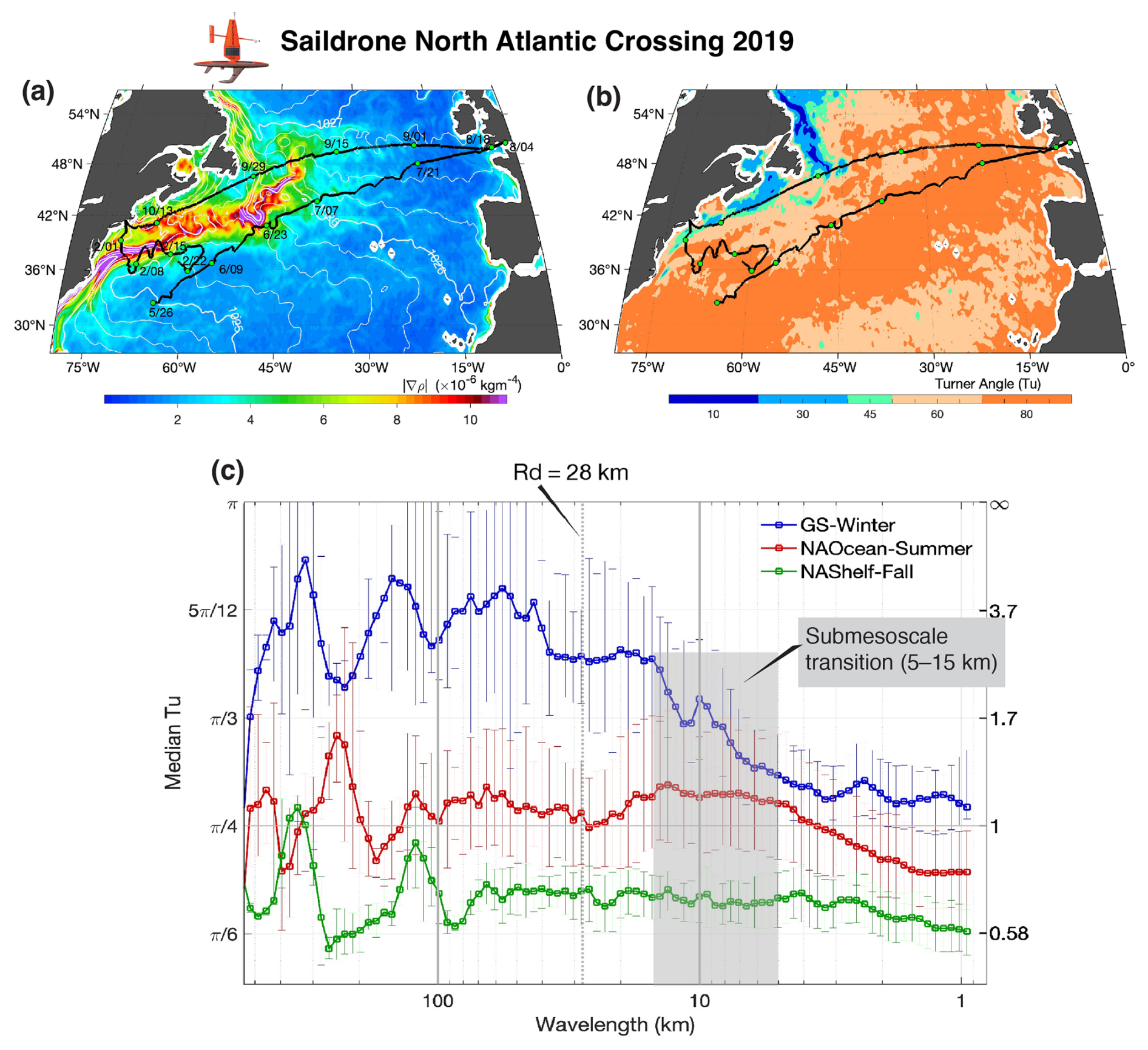
Figure 7 Thermohaline regime transition at submesoscales. (a) Sea surface density gradient magnitude and (b) Turner angle (Tu) from satellite observations with 2019 North Atlantic Saildrone tracks overlaid (black lines). Tu less than 45° (blue) indicates salinity-dominated density; Tu greater than 45° (orange) indicates temperature-dominated density. (c) Median Turner angle (left axis) and density ratio Rρ (right axis) versus wavelength computed from Saildrone measurements for three regimes: Gulf Stream winter (blue), open ocean summer (red), and continental shelf fall (green). Dashed line marks deformation radius (R_d = 28 km); gray shading indicates submesoscale transition zone (5–15 km); horizontal line marks $\mathit{Tu}=\mathit{\pi }/\mathrm{4}$ threshold. All regimes shift from temperature-dominated (Tu > $\mathit{\pi }/\mathrm{4}$) at mesoscales toward equal or salinity-dominated density gradients (Tu $\mathit{\pi }/\mathrm{4}$) at submesoscales, though the transitions is more pronounced in the open ocean summer and continental shelf fall regimes than in the Gulf Stream winter where Tu approaches but does not clearly cross $\mathit{\pi }/\mathrm{4}$. Transition sharpness varies with background conditions. Adapted from Yu (2026).

High-resolution Saildrone observations during a 2019 North Atlantic crossing reveal this thermohaline control shift (Fig. 7). At mesoscales exceeding 100 km, density gradients in the Gulf Stream and open ocean are predominantly temperature-controlled with Turner angle Tu > $\mathit{\pi }/\mathrm{4}$ and density ratio Rρ > 1, where the density ratio $R\mathit{\rho }=\mathit{\alpha }\mathrm{\Delta }T/\mathit{\beta }\mathrm{\Delta }S$ and Turner angle Tu = arctan(Rρ) together quantify the relative contributions of temperature and salinity to density, with ΔT and ΔS being temperature and salinity differences over equal distances of 350 m along the Saildrone track, α and β being the thermal expansion and haline contraction coefficients, respectively. The continental shelf, however, shows salinity already contributing significantly at these larger scales due to freshwater inputs and coastal fronts. Near 10 km Tu approaches or drops below $\mathit{\pi }/\mathrm{4}$ and Rρ approaches or falls below 1 in all three regimes, indicating a shift toward equal or salinity-dominated density gradients, though the transition is more pronounced in the open ocean and continental shelf regimes. In the Gulf Stream winter regime, Tu approaches $\mathit{\pi }/\mathrm{4}$ but does not clearly cross below it, consistent with a transition toward equal T-S contribution rather than full salinity dominance (Yu, 2026). The transition clusters near the first baroclinic deformation radius (R_d = 28 km), consistent with submesoscale dynamics emerging as the flow approaches the breakdown of purely geostrophic adjustment (McWilliams, 2016).

The sharpness of this transition is regime-dependent. In the Gulf Stream where thermal wind balance strongly dominates, Tu drops abruptly from greater than $\mathrm{5}\mathit{\pi }/\mathrm{12}$ to less than $\mathit{\pi }/\mathrm{4}$ over just 10–20 km. On the continental shelf where salinity already plays a larger role, the transition spreads over 50+ km. This regime dependence emphasizes that 10 km marks where local nondimensional ratios (Rossby number, frontogenetic sharpening versus damping, mixing versus advection) cross order unity, not a fixed geometric constant (Callies and Ferrari, 2013; McWilliams, 2016).

4.3.1 Why 10 km? Geometric and dynamical convergence

Three physical constraints converge near 10 km at mid-latitudes. First, the first baroclinic Rossby deformation radius R_d = $NH/f$ (where N is buoyancy frequency, H is ocean depth, and f is Coriolis parameter) equals approximately 10–30 km, setting the scale below which ageostrophic motions and vertical exchange intensify (McWilliams, 2016). Second, frontogenesis compresses buoyancy gradients into narrow widths approximately $U/f$ (∼ 1–10 km for typical upper-ocean velocities U ∼ 0.1–0.5 m s⁻¹ and Coriolis parameter f ∼ 5 × 10⁻⁵ s⁻¹), where strain overwhelms diffusive smoothing (Thomas and Ferrari, 2008). Third, the advective timescale $L/U$ ∼ 10 h to 1 d at 10 km becomes comparable to the diurnal and storm forcing timescales, which modulate stratification on the same window (Mahadevan et al., 2010).

This geometric convergence produces timescale convergence. At 10 km submesoscales, ${\mathit{\tau }}_{\text{adv}}=L/U$ ∼ 1–10 d, ${\mathit{\tau }}_{\text{hmix}}=L^{\mathrm{2}}/K_{\mathrm{h}}$ ∼ days to weeks (for submesoscale stirring with K_h ∼ 10–100 m² s⁻¹), ${\mathit{\tau }}_{\text{vmix}}=h^{\mathrm{2}}/K_{\mathrm{v}}$ ∼ hours to days (for active mixing with surface layer thickness h ∼ 20–50 m and enhanced K_v ∼ 10⁻³–10⁻² m² s⁻¹), and τ_f ∼ hours to days (storm passage, diurnal heating). When τ_f ∼ τ_adv ∼ τ_hmix ∼ τ_vmix, all processes compete equally. Salinity evolution becomes the joint outcome of forcing, stirring, and vertical exchange operating simultaneously rather than a hierarchy where one process dominates (Boccaletti et al., 2007; Thomas and Ferrari, 2008). This is fundamentally different from the regime separation in Sect. 4.1 and 4.2 where one timescale dominated, and salinity could be understood through that dominance.

4.3.2 Differential damping: why salinity fronts persist

Salinity achieves comparable importance to temperature in density gradients at 10 km submesoscales even in regions where temperature strongly dominates at mesoscales. The mechanism lies in differential damping of fronts. Frontogenesis sharpens both temperature and salinity gradients through strain and confluence, but only temperature fronts experience strong negative feedback from surface heat fluxes. Net surface heat fluxes, including radiative, sensible, and latent heat flux components, preferentially warm colder patches because of their lower SST, creating differential heating that erodes horizontal temperature gradients over days to weeks (Taylor and Ferrari, 2010; Mahadevan et al., 2010). Strong diurnal cycling and episodic mixing at fronts enhance this damping. The result is thermal restoring that continuously weakens temperature fronts even as frontogenesis sharpens them.

Freshwater forcing provides no comparable damping mechanism. Precipitation does not preferentially target fresh patches, and evaporation depends on atmospheric state (wind speed, humidity, air temperature) rather than on salinity itself. Salinity fronts therefore persist and sharpen through frontogenesis without the radiative damping that weakens temperature fronts (McWilliams, 2016; Jaeger and Mahadevan, 2018). In regions where temperature and salinity are positively correlated, such as the boundary between warm salty subtropical and cool fresh subpolar waters, latent heat flux damping of the temperature contrast can additionally act to strengthen the salinity gradient, providing a positive feedback that further amplified fronts relative to temperature fronts. Over the days-to-weeks timescales of submesoscale evolution (τ_adv ∼ 1–10 d, τ_hmix ∼ days to weeks), this differential damping allows salinity variance to accumulate while temperature variance degrades.

At scales below R_d where ageostrophic dynamics become strong, this differential damping shifts the thermohaline balance from temperature-dominated (Tu > $\mathit{\pi }/\mathrm{4}$, Rρ > 1) at mesoscales to equal contribution (Tu ∼ $\mathit{\pi }/\mathrm{4}$) at submesoscales (Ruddick, 1983; Rudnick and Ferrari, 1999). Equal contribution is not merely shared control but a dynamical transition: mesoscale fronts are typically thermally controlled and remain tightly coupled to the atmosphere because surface heat fluxes relax SST contrasts on O(days) timescales, limiting sustained thermal front sharpening (Taylor and Ferrari, 2010; Hausmann et al., 2017). By contrast, when submesoscale density fronts include a comparable haline contribution, the salinity component lacks an equally fast, state-dependent restoring and can therefore support sharper buoyancy gradients and stronger ageostrophic secondary circulations than temperature alone could maintain (Thomas and Ferrari, 2008; Klein and Lapeyre, 2009; McWilliams, 2016). It is worth noting that this intensification is not unbounded: as salinity gradients grow relative to temperature gradients in an initially T-dominated front, the horizontal SST gradient weakens, which ultimately reduces the frontogenetic forcing itself. Nevertheless, while the front evolves toward equal temperature-salinity contribution, ageostrophic secondary circulations can remain active. The locally generated vertical velocities at these fronts commonly reach O(10–100 m d⁻¹), approximately an order of magnitude greater than typical mesoscale vertical exchange (Balwada et al., 2018). These motions are largely confined to the upper pycnocline, where ageostrophic circulations are active, and can enhance nutrient supply, promote tracer subduction and carbon export, and contribute to mixed layer restratification. This mechanism operates most effectively in regions with strong near-surface salinity gradients such as river plume boundaries, marginal ice zones, and other freshwater-forced regimes influenced by precipitation and sea-ice melt (Mahadevan and Tandon, 2006; Boccaletti et al., 2007; Horner-Devine et al., 2015; Drushka et al., 2019; Kozlov et al., 2020; Swart et al., 2020; Coadou-Chaventon et al., 2024).

Table 3 Salinity regimes from timescale ratios.

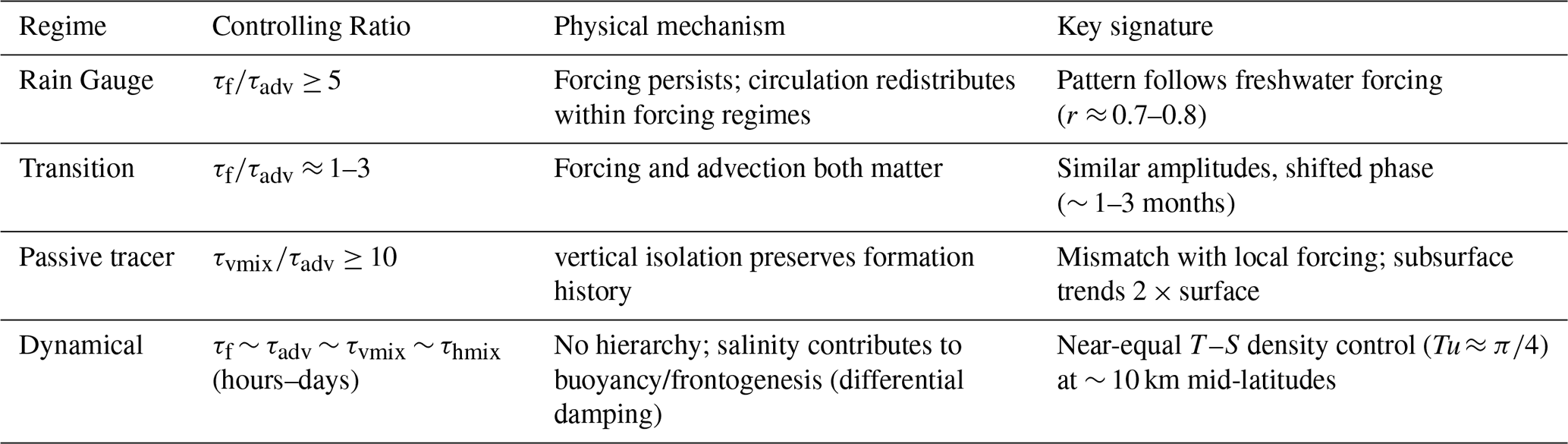
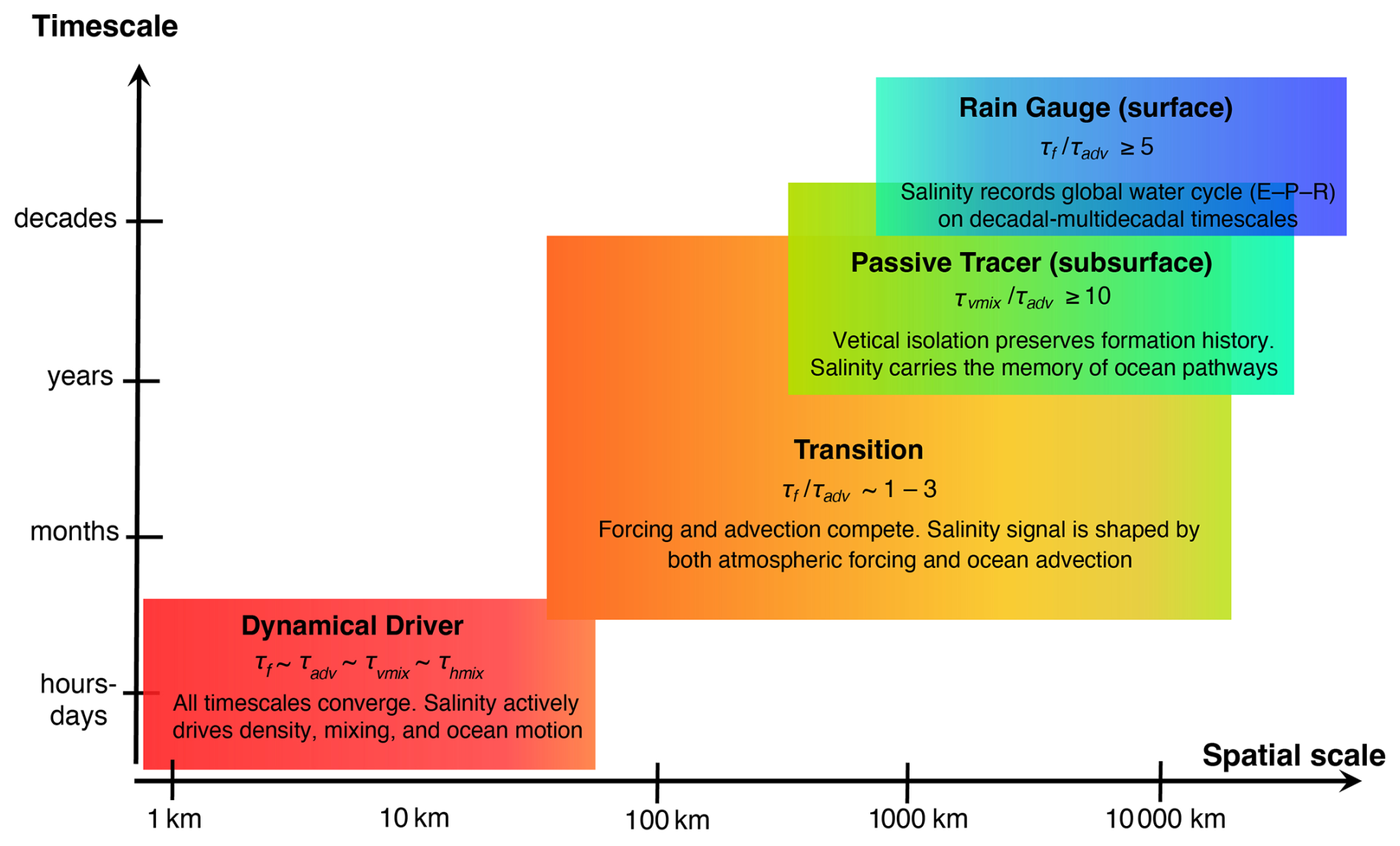
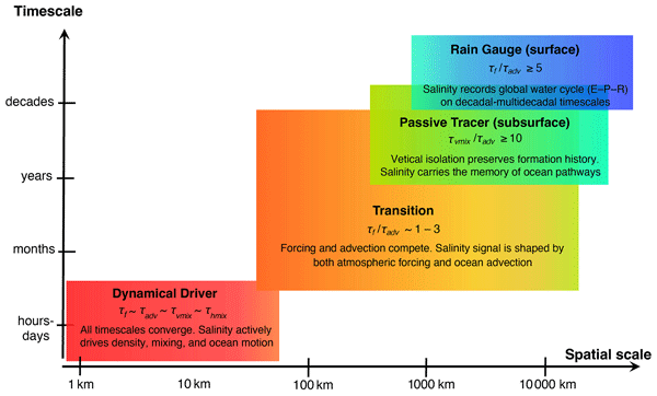
Figure 8 Salinity regime diagram. Four regimes from timescale competition (Table 3). Rain gauge (surface, cyan-blue): ${\mathit{\tau }}_{\mathrm{f}}/{\mathit{\tau }}_{\text{adv}}\ge$ 5, forcing persists, pattern tracks E−P at basin-decadal scales. Passive tracer (subsurface, yellow-green): ${\mathit{\tau }}_{\text{vmix}}/{\mathit{\tau }}_{\text{adv}}\ge$ 10, vertical isolation preserves formation history in mode waters. Transition (orange-yellow): ${\mathit{\tau }}_{\mathrm{f}}/{\mathit{\tau }}_{\text{adv}}\sim$ 1–3, forcing and advection compete, producing amplitude coherence with phase offsets over seasonal-decadal timescales. Dynamical (red): all timescales converge, and salinity actively drives density, mixing, and ocean motion. Gradient shading shows gradual boundaries. Rain gauge and passive tracer coexist at decadal-basin scales as surface and subsurface regimes, respectively. Diagram is schematic; boundaries vary with local conditions.

4.4 Synthesis: timescale ratios as regime boundaries

Across Sect. 4.1–4.3, the same message keeps resurfacing: salinity behavior does not depend on absolute spatial or temporal scales (10 km versus 100 km, or days versus years); what matters is how forcing, advection, and mixing timescales are fast or slow relative to each other. In practice, three comparisons decide how to read a salinity signal. First, does freshwater forcing change slowly enough for anomalies to accumulate where they are made (${\mathit{\tau }}_{\mathrm{f}}/{\mathit{\tau }}_{\text{adv}}$)? Second, once salinity anomalies subducted below the mixed layer, are they erased by vertical exchange or preserved as water-mass properties (${\mathit{\tau }}_{\text{vmix}}/{\mathit{\tau }}_{\text{adv}}$)? Third, are we in a regime where the process hierarchy collapses because everything happens on similar timescales? Table 3 summarizes these boundaries and what they look like in data. The four regimes are synthesized in Fig. 8 as a conceptual diagram organized by these timescale ratios, with gradient shading reflecting the gradual nature of transitions that depend on local conditions rather than fixed spatial or temporal thresholds.

The rain-gauge and passive-tracer limits are two ends of the same spectrum, but their physical basis is worth making explicit. This framework also makes the “rain gauge vs. passive tracer” behavior easier to interpret. In the rain-gauge limit, ${\mathit{\tau }}_{\mathrm{f}}/{\mathit{\tau }}_{\text{adv}}\gg$ 1, forcing persists over a spatial domain large enough that circulation recirculates water through the same forcing regio repeatedly before anomalies can escape. The rain-gauge limit therefore involves both a temporal and a spatial dimension: forcing must not only persist long enough relative to advection, but must also be spatially coherent over the circulation domain. In subtropical gyres, for example, recirculating water repeatedly samples the same evaporative forcing region, so the relevant forcing is the spatially integrated E−P over the gyre rather than the local instantaneous flux. This spatial integration amplifies the forcing signal relative to what would be expected from local E−P alone, which helps explain why subtropical salinity maxima are so robust and persistent. In the passive-tracer limit, ${\mathit{\tau }}_{\mathrm{f}}/{\mathit{\tau }}_{\text{adv}}\ll$ 1, anomalies are displaced from their formation region in both space and time. Laterally, water parcels are advected far from where they were forced before forcing changes significantly, so present-day salinity at a given location reflects conditions from a distant upstream source rather than local E−P. Vertically, once anomalies subduct below the mixed layer, they are insulated from further surface contact by the permanent thermocline and preserved along isopycnal pathways for years to decades (${\mathit{\tau }}_{\text{vmix}}/{\mathit{\tau }}_{\text{adv}}\gg$ 1). Spatial displacement between formation and observation regions is therefore the diagnostic signature of passive-tracer behavior, just as spatial coherence between salinity patterns and E−P is the signature of rain-gauge behavior.

The submesoscale case is not just another point on the same continuum; it is where the interpretation changes. When the timescales converge, salinity cannot be treated as a record of forcing or a record of upstream conditions because both are evolving on the same hours-to-days window. Through differential damping (Sect. 4.3.2), salinity contributes comparably to density and enables vertical velocities O(10–100 m d⁻¹) that ventilate the upper pycnocline, an order of magnitude stronger than mesoscale processes.

Two aspects of the regime diagram remain least well constrained. The ${\mathit{\tau }}_{\mathrm{f}}/{\mathit{\tau }}_{\text{adv}}$ ∼ O(1) transition on decadal scales, where substantial forcing amplification produces a muted salinity pattern response, still lacks a clean mechanistic attribution, as gyre adjustment, coupled variability, and changes in ventilation geometry are all plausible contributors. Additionally, although the dynamical submesoscale regime is increasingly better observed, it remains poorly represented in many climate models; how salinity-driven submesoscale overturning feeds back onto basin-scale stratification and biogeochemistry is still an open question.

5 Synthesis and Outlook

This review shows that salinity's role is set by competition among three processes: freshwater forcing, advection by ocean currents, and mixing across gradients. Sections 3 and 4 show that their balance shifts systematically with scale. At submeso–mesoscales, salinity is dynamically active because it controls density, regulates stratification, and feeds back on mixing. At seasonal–interannual scales, local forcing explains salinity evolution over only ∼ 30 % of the ocean surface; across the remaining ∼ 70 %, advection and mixing reshape anomalies before local forcing can dominate. At decadal scales, forcing control remains weak as many regions sit in transition. At multi-decadal scales, the forced imprint emerges as long-term salinity trend patterns correlate strongly (r≈ 0.7–0.8) with the climatological mean, yielding pattern amplification in which where fresh regions freshen and salty regions become saltier.

Observations over the past two decades enabled this framework. The next step is observing the scales where the balance flips. Regime boundaries are expressed through fronts, filaments, and freshwater lenses that set stratification and mixing yet are smoothed by today's SSS resolution at 40–50 km. Without resolving these features, we map large-scale patterns but miss the mechanisms creating persistence, export, and vertical penetration. The most consequential gap is therefore specific thus: sustained, global SSS at O(10 km) resolution, sampled frequently enough to track feature evolution and distinguish when salinity acts as a proxy for surface freshwater forcing, a tracer of pathways, or a driver of dynamics.

5.1 What the scale-dependent framework clarifies

The timescale competition framework clarifies three aspects of how salinity relates to forcing, circulation, and predictability.

Why spatial mismatch is informative. Interpreting salinity as a water-cycle indicator often focuses on whether it maps onto $E-P-R$. The seasonal–interannual result (forcing-dominated behavior over ∼ 30 % of area; Fig. 3) has been interpreted as evidence that salinity is unreliable across most of the ocean. But that interpretation assumes the only purpose of salinity is to mirror forcing. Sections 3 and 4 show that mismatch provides information. Where salinity departs from local forcing, water parcels have been transported or mixed before forcing accumulates locally. Those departures reveal quantities not directly observable, such as transit times, source regions, and coherence of pathways. Examples include thermocline salinity correlating with subtropical surface conditions from several years earlier, subsurface salinity maxima recording the last surface contact of a water mass, and river plume far-fields whose phase lags trace boundary-current routes. The “70 % mismatch” is signal, not noise.

Why salinity prediction depends on ocean state representation, not just atmospheric forcing. Salinity is a conservative variable in the sense that, unlike temperature, it lacks a direct negative feedback with the atmosphere: evaporation and precipitation are no controlled by the salinity state itself, so salinity anomalies are not restored toward a reference value the way SST anomalies are through surface heat fluxes. Indirect feedbacks can exist, such as a warm SST anomaly driving excess evaporation and creating a positive salinity anomaly in subtropical regions, or precipitation responses to SST further modulating salinity in the tropics. These coupling are generally secondary to the direct atmospheric restoring that acts on temperature, but they are not negligible and can reinforce salinity anomalies in some setting. This asymmetry creates memory. A model can predict rainfall anomalies correctly yet still miss salinity because the salinity at any location reflects both local forcing and the water arriving from upstream (Fig. 5). If the model misrepresents ocean currents or mixing, it delivers the wrong water to that location even when atmospheric forcing is correct. Conversely, salinity can be predictable even when rainfall is not, because water arriving today may have been formed years earlier in a distant region. This matters for practical prediction, as seasonal forecast systems can show good performance in precipitation and SST yet fail in salinity because their circulation state, pathway geometry, or mixing parameterizations are biased. Salinity forecast accuracy is therefore a coupled test: it requires both accurate forcing and ocean transport and mixing representations.

Why different studies reach different conclusions about forcing control. Basin-scale studies emphasizing robust pattern amplification and regional studies emphasizing advection and mixing are not disagreeing about physics; they examine different regime boundaries. At O(1000 km) and multi-decadal scales, forcing evolves slowly enough that circulation and mixing redistribute anomalies repeatedly and forced patterns emerge. At O(100 km) and seasonal scales, water travels large distances while forcing is evolving; local $E-P-R$ competes directly with supply from upstream. Both are correct within their domains. The distinction is not only temporal but also spatial. At basin scales, circulation redistributes anomalies within the same broad forcing regime, so the spatial pattern of salinity trends eventually reflects the spatial pattern of forcing. At regional scales, water can cross regime boundaries during transit, carrying properties formed under different forcing conditions into regions with very different local $E-P-R$.

5.2 Resolving Regime Boundaries with O(10 km) Satellite SSS

Current satellite SSS products have an effective resolution of roughly 40–50 km (Vinogradova et al., 2019; Reul et al., 2020). That scale is sufficient to map basin-scale patterns and many forced signals, but it smooths the features that often set the balance between forcing, advection, and mixing. The result is a persistent observational gap at O(10 km), the range in which salinity often transitions from a largely passive indicator of freshwater fluxes to an active dynamical driver that shapes density, stratification, and vertical exchange.

The importance of O(10 km) is dynamical, not simply a matter of detail. At these scales, three controls converge (McWilliams, 2016). First, horizontal density gradients become steep enough to drive ageostrophic secondary circulations and vertical motions of order 10–100 m d⁻¹, directly coupling lateral structure to vertical exchange. Second, salinity contrasts between adjacent water masses become large enough that salinity can rival temperature in setting density. A 0.5 psu difference can produce a density effect comparable to 2 °C, so neglecting salinity in the density budget becomes dynamically consequential. Third, freshwater-driven stratification reaches an intermediate regime where it is strong enough to inhibit routine wind mixing yet weak enough that storms can episodically overcome it. The fate of freshwater anomalies, whether they persist, mix downward, or are exported laterally, is therefore decided on storm timescales by the pre-existing frontal and stratification structure. Beyond controlling whether anomalies mix downward or are exported laterally, submesoscale processes do not merely influence but also modulate the intensity of surface salinity signals themselves. Submesoscale restratification following a mixing event can trap freshwater near the surface, amplifying surface salinity anomalies rather than diluting them. This feedback between submesoscale dynamics and near-surface stratification means that O(10 km) processes do not merely redistribute existing signals but can actively intensify them, with implications for the amplitude of surface salinity variability observed from satellites.

These controls are strongly nonlinear, and this is why coarse resolution is limiting. At 40–50 km, fronts, filaments, and freshwater lenses are blended into smooth gradients that do not represent either the sharp structures where buoyancy suppresses mixing or the well-mixed interiors where winds dominate. The relevant physics depends on the sharpness and vertical structure of the gradients, not on their spatial average. Storm response depends on the initial state. A sharp halocline at 10–20 m can resist deepening and instead sharpen under shear, whereas a more gradual stratification profile allows mixing to deepen the mixed layer and entrain freshwater from below. Freshwater over saltwater creates stratification inhibiting mixing; less mixing allows more freshwater to accumulate, strengthening stratification further (Drushka et al., 2016). This positive feedback operates only when gradients are sharp. Doubling the gradient does not double the stratification effect but can shift the regime from mixing-dominated to stratification-dominated.

A sustained O(10 km) SSS observing capability (Colliander et al., 2024) would turn these ambiguities into testable mechanisms. By tracking individual fronts and lenses through forcing events, it would quantify whether salinity stratification typically resists storm mixing or is routinely eroded, whether frontal structures sharpen through instabilities or broaden through wind stirring, and where and when the salinity contribution to density exceeds that of temperature. This is also the scale at which we can determine how much salinity variance, and therefore buoyancy variance, is currently unresolved. If the missing fraction is small, today's products and coarse models may be adequate for many climate diagnostics. If it is substantial in key regions or seasons, then parameterized submesoscale processes are not a detail but a leading source of uncertainty in regional stratification, mixing, and coupled feedbacks.

This capability matters most where freshwater forcing and gradients are strongest. River-influenced shelves and boundary currents, tropical convergence zones with patchy rainfall, western boundary current extensions with intense fronts, and marginal ice zones where freshwater and heat fluxes interact all experience large freshwater fluxes per unit area where salinity anomalies are strongest and gradients are sharpest. In these settings, O(10 km) SSS would resolve the nearshore-to-offshore transition from forcing-dominated plume cores to circulation-dominated export pathways, enabling quantitative estimates of export fractions, pathway timescales, and seasonal regime switching that current observations often describe only qualitatively. Improving to O(10 km) is not simply higher resolution but direct access to the mechanisms that control persistence, export, and vertical penetration of freshwater anomalies.

5.3 Vertical Exchange and High-Latitude Regime Shifts

Horizontal resolution addresses only part of the regime-boundary problem. Two additional observational gaps determine whether salinity anomalies remain surface-confined or become climate-relevant interior signals. Both involve transitions where competing processes cross critical thresholds, and both remain poorly constrained because current observing systems capture mean states rather than the events that drive transitions.

The first gap concerns mechanisms of vertical penetration. Subsurface salinity maxima at 100–200 m depth record surface forcing from years earlier (Fig. 6), demonstrating that anomalies can penetrate and persist. Yet penetration depends on a buoyancy competition. Wintertime cooling removes buoyancy and destabilizes the water column, while freshwater input adds buoyancy and stabilizes it. Where haline stratification is weak, as in North Atlantic subtropical mode waters, cooling deepens mixed layers through hundreds of meters and subducts surface anomalies. Where haline stratification is strong, as in the North Pacific, cooling cannot erode the fresh cap and surface anomalies remain shallow or are exported laterally. Adjacent regions with similar atmospheric forcing show markedly different penetration depths, indicating that pre-existing subsurface structure and event timing matter as much as seasonal-mean forcing (Yeager and Large, 2007).

The critical unknown is whether penetration occurs through gradual seasonal deepening or through episodic storms whose mechanical energy briefly overwhelms stratification (Dohan and Davis, 2011; Whitt and Taylor, 2017). If penetration is episodic, then a few intense storms per winter disproportionately set subduction and subsurface pathway memory. If gradual, then cumulative seasonal forcing sets penetration depth. The distinction matters for projections because climate models parameterize vertical mixing differently for gradual versus episodic processes, and future warming may strengthen haline stratification faster than it weakens thermal stratification. Testing these mechanisms requires high-frequency time series capturing individual storm responses with co-located measurements of winds, buoyancy fluxes, and vertical structure across the seasonal cycle.

The second gap concerns high-latitude regime transitions. Arctic and subpolar seas switch between long stratified periods when freshwater accumulates near the surface and brief convective episodes when mixing homogenizes hundreds of meters within days (Marshall and Schott, 1999). This switching controls whether freshwater anomalies influence deep water formation and overturning or remain surface properties. Arctic freshwater content varies by 10 000 km³ over decades, potentially affecting Atlantic overturning, but attribution requires understanding whether freshwater remains near-surface or penetrates to depth (Proshutinsky et al., 2009). Current observations are biased toward ice-free summer periods when stratification is strongest, missing winter convective events that may determine whether surface anomalies ventilate or remain trapped. Year-round sampling through under-ice platforms, moorings, and autonomous vehicles would capture regime shifts and test whether high-latitude regions are approaching thresholds where convective mixing weakens or freshwater trapping strengthens under continued warming.

These gaps highlight that resolving regime boundaries requires observing not just finer spatial scales but also the temporal variability that drives transitions between states. The processes controlling vertical penetration operate on storm timescales; the processes controlling high-latitude freshwater pathways operate on seasonal cycles that include winter conditions that remain systematically undersampled.

5.4 Model Uncertainties at Regime Boundaries

Climate model ensembles reproduce basin-scale pattern amplification yet diverge sharply in regional projections at the regime boundaries emphasized in this review. Tropical differences trace to how models represent shallow overturning and the efficiency of exporting subtropical anomalies into the equatorial band (Wang et al., 2023). Barrier layer changes depend on how models balance precipitation increases against wind-driven mixing (Pang et al., 2023; Vogt et al., 2025). High-latitude outcomes depend on whether models trigger or suppress episodic convection and how they handle ice-ocean freshwater exchange (Haine et al., 2023). These divergences concentrate where observations are currently sparse or averaged over the critical scales.

Reducing projection uncertainty requires constraining regime-boundary physics rather than perfecting basin-mean trends. O(10 km) SSS observations would constrain front-resolving buoyancy structure at the surface, while coordinated vertical observing would constrain penetration mechanisms and high-latitude switching. Together, these would enable model evaluation to move beyond climatology to process-based metrics including phase lags between forcing and salinity response, depth and strength of subsurface salinity maxima, persistence statistics of freshwater lenses, and the contribution of salinity to density at fronts.

One path forward involves state-aware parameterizations. Rather than applying uniform mixing rules tied mainly to grid spacing, models could diagnose when a grid cell is front-like with strong gradients, lens-like with strong near-surface stratification, or quiescent with weak gradients, and adjust subgrid physics accordingly (Fox-Kemper et al., 2008). This approach would encode the framework's core insight that different balances apply in different regimes.

5.5 Broader implications

The scale- and regime-dependent framework developed here extends beyond salinity. Salinity is conservative enough to preserve formation history as water parcels move, changing primarily through boundary freshwater fluxes and mixing rather than continuous air–sea exchange. This conservation makes salinity an effective tracer of pathways and memory, and it explains why the same framework applies naturally to other quasi-conservative tracers such as nutrients, dissolved gases, and isotopes (Talley, 2008). Water-cycle monitoring benefits from complementary constraints on the same forcing. At large scales and long timescales, freshwater fluxes alter both ocean mass through ocean bottom pressure and sea level and salt concentration through salinity (Liu et al., 2025). Where advection is slow relative to forcing accumulation, these constraints reinforce each other and can be used to evaluate and refine $E-P-R$ products. Where advection is fast, both mass and salinity become mixed signals of forcing and circulation, and their joint interpretation becomes regime aware rather than purely local. Observing strategies that combine gravimetry, altimetry, and high-resolution SSS offer a practical route to separating water-cycle change from redistribution by circulation, provided the key regime boundaries are resolved.

Coupled feedbacks operate through stratification. Freshwater input strengthens stratification and suppresses vertical exchange; reduced exchange can trap heat and biogeochemical properties near the surface, further modifying density structure and mixing. This feedback is inherently coupled because temperature and salinity jointly set density, density regulates mixing, and mixing sets the evolution of both fields (Zika et al., 2018; Liu et al., 2023). At basin scales the coupling can appear weak because different forcings dominate the mean budgets, but at fronts and freshwater lenses it becomes decisive on day-to-week timescales, precisely where nonlinearities are strongest. O(10 km) salinity observations target the scales where coupling is most active and where small errors in stratification and mixing can propagate upscale through biases in heat uptake, ventilation, and tracer transport.

Physical-biological connections are similarly conditioned by regime boundaries, particularly by the persistence of physical structures relative to ecosystem response times. Barrier layers and freshwater lenses create stratified surface habitats that persist for days to weeks, long enough for phytoplankton to respond but potentially too brief for higher trophic levels. Subsurface pathways transport nutrients and other tracers on multi-year routes, creating predictability only if mixing does not erase source signatures. In both cases, ecosystem predictability relates to how coherent pathways are and how fast mixing acts relative to transport. Advancing these connections involves observations that resolve the transition regimes where pathway coherence breaks down, where stratification and mixing flip between states, and where biological variability can be linked mechanistically to the evolving physical environment.

6 Concluding perspective

Over the past two decades, observations have turned salinity from a descriptive field into a physically interpretable signal. The organizing principle is competition among forcing, advection, and mixing timescales: where forcing evolves slowly relative to circulation and mixing, salinity records water-cycle change; where these timescales converge, salinity either reveals circulation pathways or actively shapes stratification and mixing. This framework explains why different studies reach different conclusions about forcing control by showing they examine different physical regimes.

The path forward is observation-driven model improvement. Resolving regime boundaries through O(10 km) SSS, event-resolving vertical time series, and year-round high-latitude sampling would distinguish among mechanisms and enable models to represent physics as state dependent rather than spatially uniform. The questions this unlocks extend beyond salinity itself: how water-cycle intensification couples with circulation change, where stratification feedbacks amplify or dampen climate responses, and how regime transitions cascade through biogeochemical cycles.

Salinity's value lies in its bridging role across climate subsystems. It connects freshwater forcing to circulation pathways and to stratification-controlled exchange, revealing how the ocean stores, transports, and transforms water-cycle anomalies and how those transformations feed back on heat uptake, interior renewal, and ecosystems. Understanding salinity across scales provides a direct route to understanding ocean climate response.