Obtaining accurate, high-frequency and long-term seawater pH data by using coupled lab-on-chip and optode sensing technologies

The marine science community requires accurate, cost-effective, and reliable pH sensors capable of long-term, stable operations in-situ from coastal to deep-sea environments. Spectrophotometric pH sensors, based on lab-on-chip (LOC) technology, offer measurement frequencies of every 10 min and provide good performance (pH difference 0.02 RMSE) relative to validation samples with long-term use. However, for applications where higher-frequency measurements are important, this maximum sample rate may be limiting, in addition to the power requirements needed to operate the sensor.

In contrast, commercially available pH optodes (PyroScience GmbH) are relatively inexpensive, consume little power and are contained within a comparatively small form-factor package, but with intense use the pH sensitive membrane can photo-oxidise, causing signal drift. The combination of LOC and optode technologies, however, can be used to provide long-term, high-frequency and high-stability in-situ pH data, but protocols to correct for sensor drift need to be developed and evaluated.

To examine sensor drift and develop protocols to account for it, we suspended two LOC pH sensors with two pH optodes at 0.5 m depth from a floating pontoon within a harbour in Southampton, UK for six months (June–December 2023). This is a highly dynamic tidal environment with substantial biofouling. The optode (AquapHOx-L-pH, PyroScience GmbH) and an independent pH sensor (Deep SeapHOx V2, Sea-Bird Scientific) measured at a high frequency (e.g., ≤ 5 min) alongside a LOC pH sensor measuring at a lower frequency (e.g., ≤ 2 h). Triplicate lab validated co-samples were collected each week, in addition to dedicated sensors monitoring the temperature, salinity, dissolved oxygen and tidal height. We find good agreement, i.e., mean ΔpH = $-\mathrm{0.022}\pm \mathrm{0.023}$ between the SeapHOx and LOC sensors (3182 data points in common), in addition to individual performances of 0.02 RMSE relative to validation samples. As expected, we found significant signal drift (e.g., generally ≤ 0.012 pH d⁻¹) and pH offsets (e.g., 0.1–0.2) with the optodes after intensive use in a high biofouling environment. However, by coupling LOC pH data to high frequency optode data, we corrected the optode signal drift/offset and achieved a similar field performance (∼ 0.02 RMSE relative to validation samples) as the SeapHOx sensor even when using ultra-low LOC pH sensor measurement frequencies (e.g., several days to weeks per LOC measurement). Overall, this work provides the oceanographic community with guidelines on how to achieve accurate, rapid, and long-term pH measurements, while also balancing power requirements, by combining two complementary pH sensing technologies.

1 Introduction

Anthropogenic carbon dioxide (CO₂) emissions are acidifying the global oceans. If emissions are not curtailed, surface seawater pH may fall by an additional 0.3, a doubling of acidity over the 21st century, by the year 2100 (Kwiatkowski et al., 2020). On a more granular level there are several processes (e.g., photosynthesis/respiration, calcification, tidal mixing, and microbial activity) that respond to even small pH fluctuations on much shorter temporal scales. Fast pH measurements can be useful in several settings e.g., dynamic estuarine and coastal regions or on ship underway systems which can experience rapid changes in the composition of the surface and near-surface seawater (Zheng et al., 2025; Aßmann et al., 2011). Furthermore, short-term anthropogenic perturbations such as runoff, upwelling and localised CO₂ emissions can create rapid pH changes (Schaap et al., 2021; Monk et al., 2021). High-frequency pH sensors can detect these transient signals that discrete sampling would otherwise miss, which highlights the need for accurate, rapid, and autonomous seawater pH sensors. Current observational targets for monitoring ocean acidification have been proposed by the Global Ocean Acidification Observing Network (GOA-ON) framework, which defines approximate uncertainty thresholds of 0.02 for weather quality data and 0.003 for climate quality data (Newton et al., 2015). These benchmarks provide a useful reference point for evaluating sensor performance.

The most accurate measurements of pH are made in a laboratory. While glass pH electrodes have been widely used for many decades, their accuracy (≥ 0.1) is limited due to junction potential drift (Dickson, 1993). Instead, the preferred method for accurate pH determination is done using a spectrophotometer (Dickson, 1993), which until recently was exclusively performed in a laboratory on land or on a ship. Seawater pH can also be determined with high accuracy indirectly by calculating pH as a function of parameters that define the carbonate system (Dickson et al., 2007). These parameters, in addition to pH, are the concentration of dissolved inorganic carbon, total alkalinity (Dickson, 1981), and the fugacity of CO₂, which is typically determined from measurements of the gas phase (Wanninkhof and Thoning, 1993). There has been significant effort within the oceanographic community to develop accurate and reliable sensors capable of undertaking these measurements in-situ and autonomously at sea.

In the past two decades, two types of technologies have been introduced that are both capable of measuring pH with high accuracy: spectrophotometric techniques and ion-sensitive field effect transistors (ISFET). The spectrophotometric technique has been implemented on a few technologies capable of autonomous in-situ deployment. The SAMI-pH sensor (Sunburst Sensors) operates on a spectrophotometric reagent-based method and offers fast (response time 3 min), low offsets (±0.003 relative to validation samples), and stable (drift <0.001 pH month⁻¹) measurements, but is only operable to depths of 600 m (http://sunburstsensors.com/products/oceanographic-ph-sensor.html, last access: 29 August 2025). A lab-on-chip (LOC) pH sensor, developed at the National Oceanography Centre (NOC, Southampton, UK), implements a spectrophotometric assay with a miniaturised fluidic manifold, valves, pumps, and electronics in a portable device (Aßmann et al., 2011; Liu et al., 2006; Martz et al., 2003). LOC pH sensors can make highly accurate measurements (uncertainty <0.01 at pH 8.0) for several months at sea (Mowlem et al., 2021; Rérolle et al., 2014). They are also capable of operating at 6000 m (Yin et al., 2021). While they consume little reagent (ca. 3 µL) and produce little waste (ca. 2 mL) per sample (Yin et al., 2021), management of reagent/waste volumes and power consumption can limit measurement frequency during long deployments. This LOC pH sensor has recently become commercially available (https://www.clearwatersensors.com/ph-sensor.html, last access: 29 August 2025). Conversely, pH ISFETs, which have been used on commercially available instruments such as the SeaFET and SeapHOx (Sea-Bird Scientific) for over ten years, are the most used instruments for oceanographic pH measurements. ISFETs were first adapted for pH measurements in the deep sea over twenty years ago (Shitashima et al., 2002). Their use in oceanography greatly expanded after rigorous evaluation of the DuraFET (Honeywell) pH ISFET sensor (Martz et al., 2010). The Nernstian response of the DuraFET to changes in seawater salinity and pH, in addition to best practices, were later established (Bresnahan et al., 2014). This technology has been implemented in the SeaFET instrument for measurements of pH alone, and in the SeapHOx instrument, which is capable of measuring pH, dissolved oxygen, conductivity, temperature, and depth, with a modified version operating to depths of up to 2000 m (Johnson et al., 2016). The manufacturer reported instrument offsets relative to validation samples is ±0.05 with a precision of 0.004 (https://www.seabird.com/, last access: 29 August 2025). The performance can be further improved for months-long deployments by modifying the instrument with a reservoir of TRIS buffer and an additional pump to allow self-calibration (Bresnahan et al., 2021). Nonetheless, the ISFET-based pH sensors are known to have long-term electrode signal drift and require long conditioning times within the sensing environment, e.g., 1–2 d periods from the manufacturer, whereas others recommend longer ≥5 d conditioning periods (Saba et al., 2019; Bresnahan et al., 2014). The conditioning time is dependent on the reference electrode configuration e.g., the Deep SeapHOx V2 only has an external Ag/AgCl reference electrode whereas the shallow-water SeapHOx and SeaFET units utilise an external Ag/AgCl reference electrode in addition to an internal Ag/AgCl (gelled electrolyte) reference electrode. As a result, the Deep SeapHOx V2 sensor (used in the present study) requires a longer conditioning time in the sensing environment and the salinity correction to the pH data becomes quite important.

Two practical limitations to the more widespread use of these sensors are their size and power consumption. The commercial versions of the LOC pH sensor, with a cartridge of reagents, are cylinders 56 cm long and 16 cm in diameter. Power consumption is 1.8 W during measurement (e.g., ∼ 1000 Joules of energy per sample) and 6 mA in sleep mode in between measurements. The SeapHOx is 559 mm × 129 mm × 283 mm (Sea-Bird Scientific). Power consumption during measurement is smaller, at a maximum of 0.4 W. Both instruments have been equipped on autonomous platforms, but the volume that these instruments require, and the power that they consume, limits the space and power available for other instruments on the platform (Takeshita et al., 2021; Saba et al., 2019; Hammermeister et al., 2025). In comparison, the pH ISFET instrumentation on an Argo profiling float uses a reported 19.7 J sample⁻¹ (Bittig et al., 2019).

Newly available pH optode sensors (e.g., AquapHOx-L-pH; PyroScience GmbH) have recently begun to be explored for oceanographic applications (Wirth et al., 2024; Staudinger et al., 2019, 2018; Fritzsche et al., 2018; Monk et al., 2021). While these sensors are prone to signal drift (manufacturer reported drift <0.005 pH d⁻¹) as a result from deterioration of the pH sensitive coating, they can provide rapid (<1 min per measurement) pH data. The sensor has an internal rechargeable battery, and the manufacturer suggests it can operate for 2 months sampling every 10 s (https://www.pyroscience.com/en/products/all-meters/aquaphox-l-ph, last access: 29 August 2025). The physical size of the sensor is small (37.5 cm long and 6.3 cm in diameter) allowing for easy integration onto autonomous vehicles, and they can be procured with both shallow (100 m) and deep-sea (4000 m depth rated) housings. Furthermore, provided there is access to the sensor, the consumable pH caps are easily changed, and the calibration procedure is straightforward enough that it can be carried out in the field. Recent work has provided guidelines for the oceanographic community regarding the calibration of the optode-based pH sensors with implications for field test data, but it indicates that the sensor is best suited for short-term (i.e., weeks to months) deployments where drift is less of a problem (Wirth et al., 2024). Nonetheless, these small optode-based sensors have the capacity to be a powerful tool for oceanographic research, but protocols need to be developed to improve their long-term accuracy.

In this paper, we demonstrate the efficacy of a combined system featuring both a LOC spectrophotometric pH sensor and an optode. We demonstrate the ability of this combined sensor package to provide accurate, rapid, and long-term pH data against an independent pH sensor (SeapHOx) during a 6-month shallow field test. We also provide a data analysis method to correct for signal drift and offset, in addition to discussing the balance between power and accuracy of the combined system during a long-term field deployment. The assessment undertaken offers guidelines for the oceanographic community on how to obtain accurate, rapid, and long-term seawater pH data.

2 Materials and Procedures

2.1 Field test site and pH sensor setup

To demonstrate the sensor combination, we deployed sensors at a shallow test facility within a harbour at the NOC in Southampton, UK (50°53^′33.8496 N, −1°23^′40.7148 E) from late-June until mid-December 2023. The NOC is located at the head of Southampton Water, a tidal estuary site that is characterised by mixing between the marine waters of the English Channel and two principal chalk freshwater rivers (the River Itchen and the River Hamble). The quay is a busy port area that can have multiple commercial and research ships enter/exit each day. Three pH sensors (described below) were suspended at fixed points from a floating pontoon to a fixed depth of ca. 0.5 m below the seawater surface. A pressure (depth) sensor (EXO2 multi-parameter sonde; YSI) was suspended from a fixed point that did not rise/fall with the pontoon.

The relevant pH sensor specifications are provided in Table 1. The LOC sensor, manufactured at the NOC (Yin et al., 2021), is rated for deep-sea use and was powered by an external rechargeable lead-acid battery that was stored inside a waterproof box above the location where the sensor was secured to the pontoon. The battery was swapped at regular intervals (i.e., every four days). The reported accuracy and resolution of the LOC sensors are < ±0.009 and <0.001, respectively (https://www.clearwatersensors.com/ph-sensor.html, last access: 29 August 2025). The shallow-rated optode sensor (AquapHOx-L-pH; PyroScience GmbH) has an internal rechargeable Li-ion battery. The reported accuracy and resolution from the manufacturer are ±0.050 and 0.003, respectively (https://www.pyroscience.com/en/products/all-sensors/phcap-pk8t-sub, last access: 3 September 2025). The SeapHOx sensor (Deep SeapHOx V2; Sea-Bird Scientific) is rated for deep-sea applications and is powered by internal non-rechargeable batteries (https://www.seabird.com/deep-seaphox-v2-ocean-ct-d-ph-do-sensor/product-downloads?id=60762467726, last access: 29 August 2025). Specifically, this sensor consists of two parts: (1) a pH sensor and (2) a conductivity-temperature-depth and dissolved oxygen (CTD-DO) sensor. These are physically connected using a support clamp and the relevant CTD-DO data feed into the pH sensor calculation. The reported accuracy and resolution from the manufacturer are ±0.050 and 0.004, respectively.

Table 1 Sensor dimensions, weight (in air), depth rating, accuracy, resolution, drift, and cost indication.

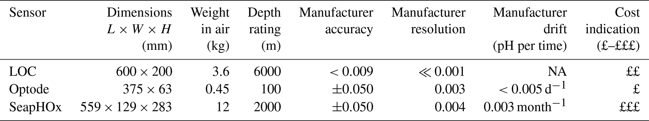
NA – not available.

The sensor dimensions reported in Table 1 are of the exterior housing to give an indication of the overall footprint that is relevant to physical integration onto vehicles/platforms, but the optode and SeapHOx were operated as fully autonomous systems whereas the LOC sensor utilised an external power supply. The optode sensor was deployed side-by-side with the LOC sensor by simply attaching the optode to the exterior housing of the LOC sensor (refer to Fig. 1a). Cable zip ties were used to achieve this and never failed in our tests, but a more robust attachment could easily be constructed. The two combined LOC + optode sensors and the SeapHOx sensor were spaced ca. 0.5 m apart from each other.

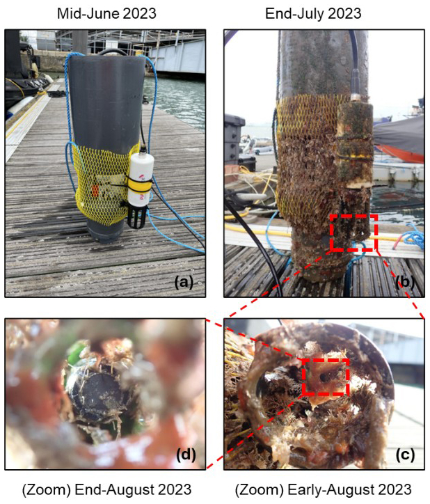
Figure 1 Pictures taken during phase 1 showing (a) clean combined optode + LOC sensor package at start of deployment in mid-June 2023 for reference, (b) combined optode + LOC sensor package at the end of July 2023 with significant bioaccumulation, (c) close-up on optode external protective cage in early-August 2023, and (d) zoom-in on pH cap protective cage showing the pH-sensitive optode surface at the end of August 2023.

2.2 Data analysis

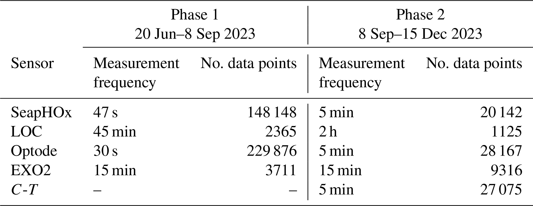
To test the impact of measurement frequency on the resulting pH data, the sample rates of the pH sensors (i.e., SeapHOx, LOC, and optode) were changed halfway through the field trial (refer to Table 2). During phase 1 (20 June–8 September 2023) the SeapHOx and optode sensors were deployed with rapid <1 min measurement frequencies, whereas the LOC sensor had a significantly lower measurement frequency of every 45 min. During phase 2 (8 September–15 December 2023) the measurement frequencies of the SeapHOx and optode sensors were lowered to sample every 5 min, and the LOC sensor was lowered to measure every 2 h. A YSI EXO2 multi-parameter sonde was utilised to obtain tidal height data every 15 min throughout the entire study. An independent C-T (conductivity and temperature) sensor (microCAT C-T, Sea-Bird Scientific), deployed during phase 2, measured every 5 min and provided a back-up in case of failure of the CTD-DO portion of the SeapHOx sensor.

Table 2 Deployment dates (phase 1 and phase 2), measurement frequencies, and number of data points collected for each sensor.

The raw data from the LOC pH sensor was post-processed as described previously (Yin et al., 2021) using in-situ salinity and temperature data from an independent C-T sensor. The raw data from the optode pH sensor was also post-processed for salinity and temperature from an independent C-T sensor using a Microsoft Excel-based calculator provided by the manufacturer (PyroScience, Münevver Nehir-Pellengahr, personal communication, 28 May 2025). Lastly, the SeapHOx sensor output processed pH values using the on-board salinity and temperature measured from its CTD. Therefore, all pH data presented here has been adjusted to account for the known salinity and temperature at the time of measurement. The pH values are reported on the total proton scale (pH_T), and no signal averaging was done to any data within the present study.

2.3 Sensor calibration

The LOC sensor, manufactured in 2022, is a calibration-free method wherein during the manufacturing process a one-off correction to the optical system is applied to account for the wavelength non-specificity of the LEDs (Yin et al., 2021). The optode sensor was calibrated following the manufacturer's recommended procedure prior to deployment. Specifically, a fresh optode pH cap (PHCAP-PK8T-SUB, PyroScience GmbH) was soaked in the manufacturer-provided buffer reagents for an hour before following the calibration guide on the software. This was a two-point buffer (pH 2 and pH 11) calibration and was done once before phase 1 and once before phase 2 when a new optode pH cap was installed. The SeapHOx sensor was calibrated in September 2021 by the manufacturer. The pressure (depth) sensor was re-zeroed on land prior to deployment. The combined conductivity and temperature sensor (microCAT C-T; Sea-Bird Scientific) was calibrated in July 2017 by the manufacturer.

2.4 Lab pH validation process

To validate the results from the pH sensors, triplicate discrete seawater co-samples (n=44, i.e., 132 samples total) were manually collected in 60 mL polypropylene syringes (Terumo Eccentric Luer-tip 3-part syringe) adjacent to the sensor inlets and measured in a lab immediately following collection using a previously outlined procedure (Yin et al., 2021). The discrete samples were not poisoned, the time between co-sampling and lab measurements was ≤10 min (i.e., the harbour was directly accessible from the NOC), and the time of the discrete sample was noted upon collection (i.e., the collection time was used for comparison to sensor data). Each triplicate discrete sample was copiously flushed through a 10 cm water jacketed glass optical cell, where the temperature was maintained at 20 °C, and 5 µL injections of 4 mM purified meta-Cresol Purple (mCP) was added to ca. 8 mL of sample on a Cary 60 UV-vis (Agilent Technologies) spectrophotometer. The average of each triplicate co-sample was taken. The mean and standard deviation of the difference between replicate co-samples was 0.007±0.008. The total uncertainty of the spectrophotometric measurement procedure used in this study was calculated to be 0.005, which includes individual uncertainties for the temperature, absorbance, baseline correction, deuterium lamp, and the calculation of pH from spectrophotometric data (Carter et al., 2013; Yin et al., 2021). The salinity of each discrete sample was also measured using a commercial conductivity meter (WTW Cond 3110) and probe (WTW TetraCon 325).

2.5 Sensor maintenance

Routine maintenance was carried out when sensors were retrieved for data download and as needed. LOC: The sample inlet filter for the LOC sensor was changed every week during the initial three months (phase 1) but remained unchanged during the final three months (phase 2). The sample inlet filter was left unchanged during phase 2 to assess if biofouling impacted the pH signal. The LOC sensor waste bag was emptied at opportunistic times throughout the study. Power was supplied to the LOC pH sensor via a rechargeable lead-acid battery, which was swapped out with a fresh battery at regular intervals (i.e., every four days) to avoid disruption to data collection. During week 10, the LOC pH sensor was flushed for 5–10 min each with a sequence of solutions (i – 10 % Decon-90 cleaning solution, ii – ultrapure water, and iii – filtered seawater) to clean the microfluidic channels as a result of the significant biofouling encountered. Optode: The rechargeable internal battery charge level was checked during data transfer (and opportunistically recharged). A copper mesh fabric was installed around the outer protection cage of the optode sensor at the beginning of August to help minimise the significant bioaccumulation observed and was subsequently removed near the beginning of Phase 2 (mid-September) due to the deployment of a second optode pH sensor which was equipped with an anti-fouling copper mesh guard. The spent optode cap from phase 1 was replaced with a freshly lab-calibrated optode cap for phase 2 following the manufacturer's guidance. SeapHOx: Prior to deployment the SeapHOx sensor wet cap was filled with seawater from the test site for one week to condition the sensor. The small pinhole on the attached CTD-DO half was regularly cleaned of accumulated biomass during phase 2 to prevent air buildup within the sensor. The sensor was equipped with anti-fouling technology utilising a flow-path to extend deployment durations in high-fouling environments. The on-board batteries for both the components of the SeapHOx sensor (i.e., pH and CTD-DO) were replaced on 13 November 2023, and the sensor housing was cleaned during this process. EXO2: The internal D-cell batteries of the pressure (depth) sensor were replaced at regular (monthly) intervals. Minimal fouling was observed on this sensor due to its deeper deployment depth. C-T: No maintenance was carried out on the microCAT C-T sensor after deployment.

3 Results and Discussion

3.1 Sensor performance: phase 1

The manufacturer of the optode pH sensor claim that the battery can last between 2 to 6 months with a measurement interval between 10 to 60 s, respectively. In our testing, the optode sensor's battery was never depleted even during periods of high measurement frequency. When data was downloaded from the sensor the internal Li-ion battery did trickle charge, but this never lasted longer than 10 min. For reference, the manufacturer indicates that the sensor can be fully recharged in 2 h.

The combined LOC + optode pH sensor package (Fig. 1a) provided near continuous data collection over the first three-month period (phase 1). Phase 1 occurred during the warmer summer months (i.e., the surface water temperature was relatively constant around 20 °C) and, due to the fixed 0.5 m deployment depth, we observed significant bioaccumulation on the sensors. Pictures taken during July and August show the challenging biofouling environment the pH sensors operated in (refer to Fig. 1b–d highlighting biofouling on the optode sensor). A deeper look at the chemical and physical drivers that affected the seawater pH during this study is provided in Sect. S1 in the Supplement.

During phase 1 of the study the optode measured at a high frequency, every 30 s, whereas the LOC measured at a low frequency every 45 min. An overview of the phase 1 optode and LOC pH sensor data, alongside discrete lab validated co-samples, are provided in Fig. 2. The LOC data showed good agreement with the discrete lab validated co-samples throughout phase 1, with an average offset relative to discrete lab validated co-samples of $-\mathrm{0.012}\pm \mathrm{0.014}$ (n=15). Similar data quality has been observed from the LOC pH sensor in the past from the same deployment site (Yin et al., 2021). The optode sensor showed relatively good agreement with discrete co-samples within the first month, i.e., 0.024 ± 0.014 (n=10), but thereafter its signal continuously drifted away from the LOC and discrete co-sample pH values until the end of phase 1. Signal drift of 0.002 d⁻¹ and offsets of e.g., 0.1 to 0.4 have been reported previously for optode-based pH sensors deployed in the field (Delaigue et al., 2025; Wirth et al., 2024).

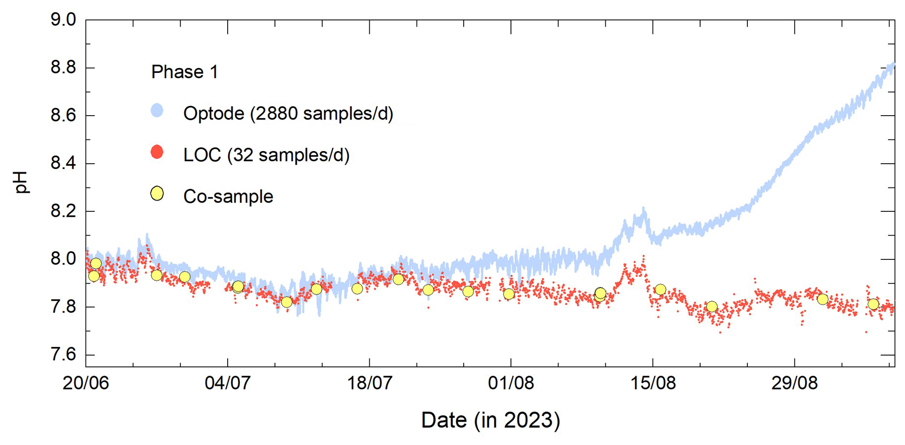
Figure 2 Overlay of optode (light blue filled circles), LOC (red filled circles), and discrete lab validated co-sample (yellow filled circles) pH data during phase 1.

It should be noted that we intentionally let the optode signal drift away from the LOC reported values (rather than recalibrate or replace the sensing foil) to examine the impact on measurement performance (i.e., baseline vs. response drift). Interestingly, even with a drifting baseline signal, when zoomed in the optode still follows features that are seen with the LOC sensor (Sect. S2 in the Supplement). There are largely two factors at play that could cause this significant signal drift. Firstly, the high measurement frequency employed could photo-oxidise the pH sensitive coating causing rapid deterioration of the pH cap coating. These pH caps are a consumable component of the sensor device and are easily calibrated and replaced when worn. If the device can be retrieved and replenished with a freshly calibrated pH cap (as done in the present study), this can mitigate this issue, but this represents a problem when deployed in remote locations or on moving platforms. Secondly, the significant biofouling environment encountered could disrupt the long-term quality of the data. We are unable to confidently identify which of these has a greater effect but acknowledge that both factors were at play.

3.2 Sensor performance: phase 2

At the end of phase 1 the optode was cleaned and a new freshly calibrated pH cap was installed. The sensor was then re-deployed for phase 2 of the study. Phase 2 occurred during the end of 2023 where the surface water temperature decreased from ca. 20 to ca. 8 °C. As a result, there was less bioaccumulation on the sensors during this period. Furthermore, the measurement frequency was reduced to every 5 min for the optode and 2 h for the LOC sensor. The measurement frequency was reduced during phase 2 to examine the effect of sample frequency on the drift of the optode (e.g., via photodegradation) and to conserve battery during the colder months of the deployment. An overview of the phase 2 optode and LOC pH sensor data, alongside discrete lab validated co-samples, are provided in Fig. 3. Interestingly, from nearly the start we observed a signal offset between the optode and the LOC data. This offset is prevalent throughout the majority of phase 2. Recent work has shown that using a three-point buffer calibration (in lieu of a two-point buffer calibration) can be beneficial in reducing signal offsets and improving absolute accuracy for optode-based pH sensors in laboratory settings, but for field deployments discrete co-samples are required to maintain this level of sensor performance (Wirth et al., 2024). The LOC pH data showed good agreement with the discrete lab validated co-samples, displaying a difference of $-\mathrm{0.024}\pm \mathrm{0.011}$ (n=10). While the mean bias (pH offset) has doubled from −0.012 to −0.024 relative to discrete samples, this could be a result of the significant biofouling encountered and the fact that during phase 2 the LOC sample inlet filter was left unchanged (whereas during phase 1 it was replaced every 1–2 weeks). Furthermore, the reduced measurement frequency within phase 2 does not appear to show the same rate of significant signal drifting as encountered towards the end of phase 1. This could be a result of the colder temperatures experienced in phase 2 where the temperature decreased gradually from ca. 20 to ca. 8 °C or an outcome of the lower measurement frequency. As in Phase 1, optode sensor pH sensitivity/response appeared to be comparable to that of the LOC sensor despite the signal offset between them. Based on this observation we propose that periodic signal correction (e.g., using LOC sensor measurements) could restore and maintain the quality of the high frequency optode sensor signal during long deployments. A correction method that leverages the low-frequency, stable LOC pH sensor data is described below.

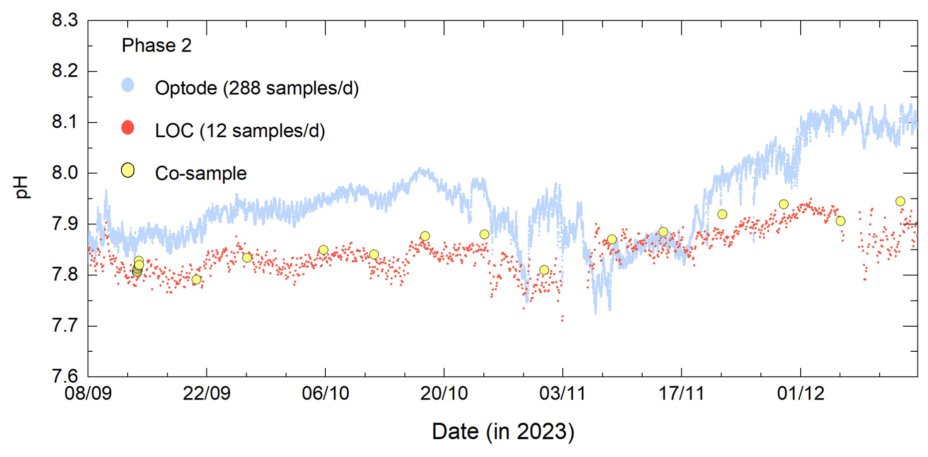
Figure 3 Overlay of optode (light blue filled circles), LOC (red filled circles), and discrete lab validated co-sample (yellow filled circles) pH data during phase 2.

3.3 Optode correction method

Linear corrections to post-deployment data have been previously utilised for oceanographic pH (Wimart-Rousseau et al., 2024; Hemming et al., 2017; Takeshita et al., 2021) and dissolved oxygen (Miller et al., 2024; Gerin et al., 2024) data. In principle, the correction method applied should take a conservative approach by aiming to remove known sources of irregularity (e.g., drifts or offsets) while preserving real variability in the sensor data. To accomplish this, our methodology leverages a LOC-based pH sensor which can sample at a low frequency to conserve battery, while operating a pH optode device that may be prone to drifting/offsets, but which can sample at a much higher frequency to resolve fast pH changes. A linear rate correction was obtained by fitting a line to two LOC data points over a specified interval in time (e.g., every 1 week, every 1 d, every 1 h) and then adding the residuals from the high frequency optode data onto this gradient. In effect, this adjusts the gradient of the optode dataset to match that from the LOC dataset while preserving the high-frequency fluctuations from the original optode data. The choice of LOC measurement interval was adjusted in this study to determine the impact of the choice of interval on the remaining error of the corrected optode data. We evaluated several alternative correction methods e.g., offset correction, moving average smoothing, multi-point line fitting, etc. that can be seen in Sect. S3 in the Supplement. While these methods produced comparable results in some cases, the method described here provides the most favourable balance between correction performance, simplicity of implementation and a reduced LOC sampling frequency.

A brief mathematical expression of the correction process follows. A line was fitted between two LOC data points collected with the correction interval between then. This is expressed in Eq. (1):

$$\begin{array}{}\text{(1)}& {\mathrm{pH}}_{\mathrm{LOC}}^{\mathrm{Fit}}\left(t_{\mathrm{i}}\right)=m_{\mathrm{LOC}}\left(t_{\mathrm{i}}-t_{\mathrm{LOC}\mathrm{1}}\right)+b_{\mathrm{LOC}}\end{array}$$

where m_LOC is the slope of the LOC data, t_LOC1 is the start of the interval (based on the first LOC data point), b_LOC is the intercept of the LOC data fit to time, and t_i is the time of the individual sample to be corrected. It is worth noting here that this simple two-point line fit is used to mimic physically changing the LOC measurement frequency. For example, during phase 2 when a 2 h measurement frequency was used, if the fitting correction interval was set to 24 h, this would imply there are 12 points within that period yet only two of them are used in the line fit (i.e., the first and last data points).

A linear regression was also done to extract the best fit line from the raw optode data within the same correction interval (but in this case all the optode data was used) and is expressed in Eq. (2):

$$\begin{array}{}\text{(2)}& {\mathrm{pH}}_{\mathrm{Optode}}^{\mathrm{Fit}}\left(t_{\mathrm{i}}\right)=m_{\mathrm{Optode}}\left(t_{\mathrm{i}}-t_{\mathrm{LOC}\mathrm{1}}\right)+b_{\mathrm{Optode}}\end{array}$$

where m_Optode is the slope of the raw optode data, t_LOC is the start of the interval (based on the first LOC data point), and b_Optode is the intercept of the optode data.

Next, the residuals (r) from the optode dataset are computed. These are the deviations of the raw optode data points from its own linear trend. The residuals are expressed in Eq. (3) as:

$$\begin{array}{}\text{(3)}& r_{\mathrm{Optode}}\left(t_{\mathrm{i}}\right)={\mathrm{pH}}_{\mathrm{Optode}}\left(t_{\mathrm{i}}\right)-{\mathrm{pH}}_{\mathrm{Optode}}^{\mathrm{Fit}}\left(t_{\mathrm{i}}\right)\end{array}$$

where pH_Optode(t_i) is the original raw optode data point and ${\mathrm{pH}}_{\mathrm{Optode}}^{\mathrm{Fit}}\left(t_{\mathrm{i}}\right)$ is expressed as above in Eq. (2).

Therefore, the corrected pH (pH_Corrected) can be mathematically defined in Eq. (4), wherein the linear fit from the LOC data is added to the computed residual signal from the optode data.

$$\begin{array}{}\text{(4)}& {\mathrm{pH}}_{\mathrm{Corrected}}={\mathrm{pH}}_{\mathrm{LOC}}^{\mathrm{Fit}}\left(t_{\mathrm{i}}\right)+r_{\mathrm{Optode}}\left(t_{\mathrm{i}}\right)\end{array}$$

The expanded, final form of the fitting method can be mathematically expressed as below in Eq. (5).

$$\begin{array}{}\text{(5)}& \begin{array}{rl}{\mathrm{pH}}_{\mathrm{Corrected}}& ={\mathrm{pH}}_{\mathrm{Optode}}\left(t_{\mathrm{i}}\right)+\left(m_{\mathrm{LOC}}-m_{\mathrm{Optode}}\right)\\ & \cdot \left(t_{\mathrm{i}}-t_{\mathrm{LOC}\mathrm{1}}\right)+b_{\mathrm{LOC}}-b_{\mathrm{Optode}}\end{array}\end{array}$$

This approach maintains the low-frequency trends of the LOC while also including the high frequency features of the optode, and as a result was the chosen method used for data correction.

Figure 4 shows an example of this correction process, applied during one 24 h correction interval. The LOC data are shown as the unfilled red circles and the two LOC data points used in the linear fit are exemplified by two filled red circles at the start/end of the window. There are 33 LOC data points within this 24 h window but only the two filled red circles are used to generate the linear fit to the LOC data (illustrated as the solid red line). Again, the LOC linear fit sets the gradient to which the optode data will be corrected. Next, the light blue circles are the raw optode data, and for reference, there are 2898 optode data points within this same 24 h window. The solid black line is the linear fit to the entire set of this optode data. Finally, the corrected optode data, using Eq. (5), are shown as the dark blue circles. In this instance, the offset that the entire raw optode data exhibited was corrected. Three discrete co-sample data points are also overlaid as filled yellow circles. We can see that the corrected optode data are in much better agreement with these discrete samples. Therefore, a 24 h correction interval (i.e., a LOC data point once per day) was sufficient to improve the optode sensor data to be in agreement with LOC pH data and discrete co-samples. Overall, this shows the power of simply using a single LOC data point once per day to mitigate any signal drift/offset in the optode dataset.

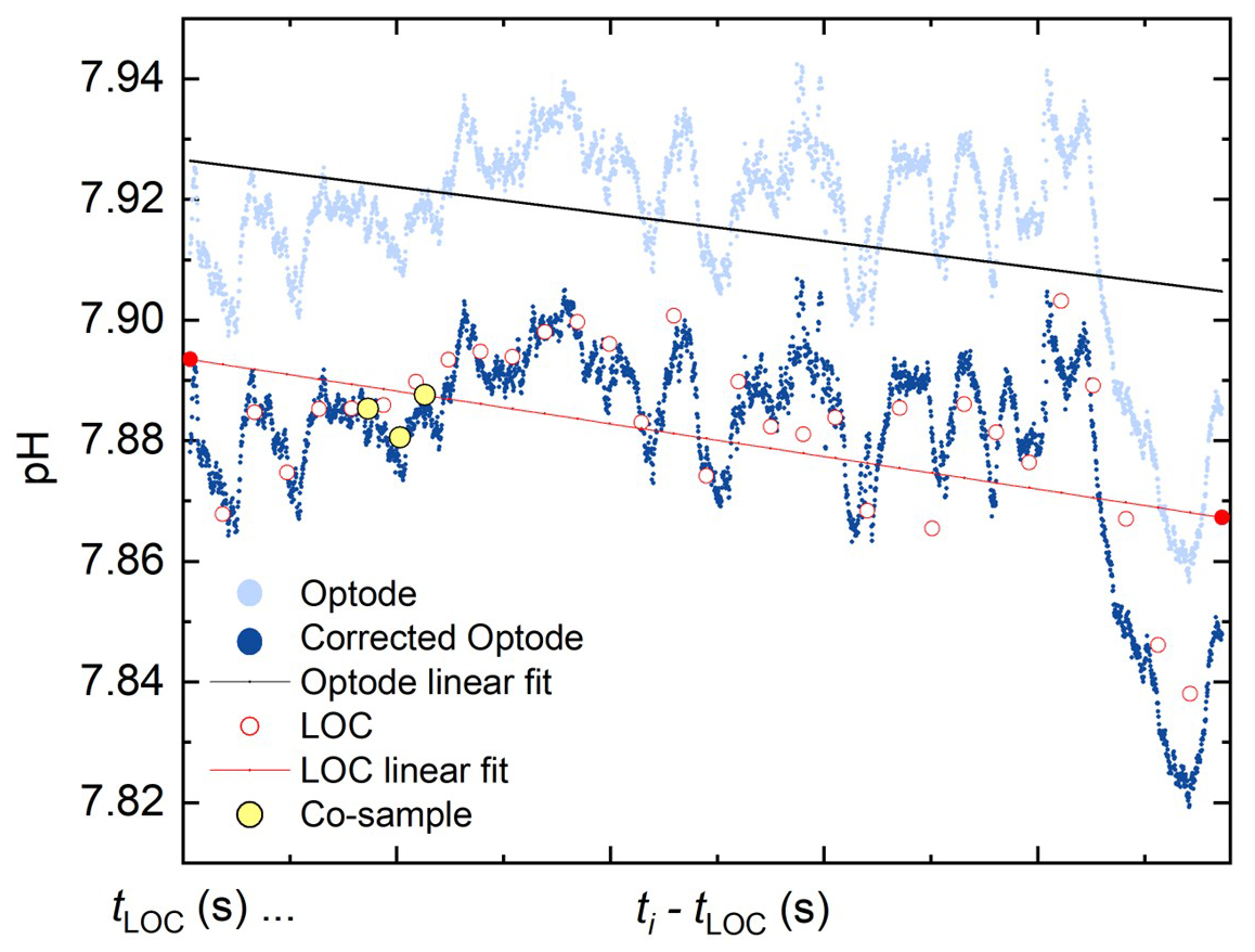
Figure 4 Exemplar data from early July 2023 showing a 24 h period used to illustrate the correction method applied to the optode dataset. Overlaid are the raw optode data (light blue circles), corrected optode data (dark blue circles), linear fit to raw optode data (solid black line), LOC data (unfilled red circles), linear fit to LOC data (solid red line), and discrete co-samples (filled yellow circles). Note: the two filled red circles are the start and end LOC data points used in the LOC linear fit.

While the example in Fig. 4 uses a 24 h correction interval, we repeated the analysis for several different correction intervals to evaluate the effect of the interval on the agreement between corrected optode data and lab-validated samples. The data in Table 3 report the results of the corrected optode pH sensor relative to discrete lab validated co-samples. Specifically, sensor performance in the present work is evaluated using three statistical metrics relative to the independent discrete co-sample reference measurements, i.e., the mean error ($\stackrel{\mathrm{‾}}{x}\mathrm{\Delta }$pH), the standard deviation of the error (1σ±ΔpH), and the root mean square error (RMSE ΔpH). The mean error (i.e., $\stackrel{\mathrm{‾}}{x}$) represents systematic bias (offset) relative to the reference measurements, while the standard deviation (1σ) reflects the spread of residual differences and therefore the measurement precision. The RMSE incorporates both the systematic bias and the random variability and therefore provides a combined estimate of total measurement error. As can be seen the performance improved with more frequent correction intervals (i.e., higher LOC measurement frequencies). A correction every four weeks was sufficient to dramatically improve the performance of the entire set of uncorrected raw data from a difference of +0.111 ± 0.172 (n=44) to +0.021 ± 0.034 (n=44), which is within the reported specification of the SeapHOx pH sensor. A correction every 1-week further improved the difference to −0.007 ± 0.024 (n=44), but improvements largely plateaued at higher LOC measurement frequencies e.g., a correction every 24 h produced a difference of $-\mathrm{0.011}\pm \mathrm{0.017}$ (n=44). Effectively, the performance of the optode sensor approached the performance of the LOC sensor itself as the correction interval approached the maximum sampling rate of the LOC pH sensor (i.e., in this instance every LOC data point is used to correct optode data; this is reported in Table 3 as All data).

Table 3 Performance of the optode sensor, relative to discrete lab-validated co-samples, is reported as the mean sensor error ($\stackrel{\mathrm{‾}}{x}\mathrm{\Delta }$pH), standard deviation of the error (1σ±ΔpH), and the root mean square error (RMSE ΔpH). The number of samples (n) for determining these metrics were n=44 for all correction intervals.

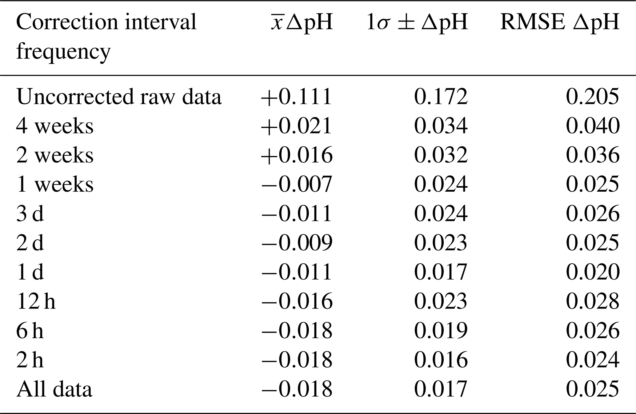
It is worth noting here that there is a local minimum observed in $\stackrel{\mathrm{‾}}{x}\mathrm{\Delta }$pH at the 2 d point and in 1σΔpH at the 1 d point. There are two possible explanations for this behaviour. Firstly, the starting point for the correction was always done from the very first LOC data point, and subsequently the fitting windows all spanned according to that single starting point. To account for this, we examined the dataset using a range of different starting points and determined it has a relatively small impact on the overall result (Sect. S3 in the Supplement). Secondly, the two-point fitting method applied to the LOC data is subject to effects in the form of which data points are used within the line fit. For example, (referring to Fig. 4) simply moving the LOC fit from the last data point (33rd data point) to the previous data point (32nd data point), would produce a significantly different gradient (note: this is not the case with the raw optode data wherein the entire dataset within the fitting window is taken into account with its linear fit). The latter point is likely to have a large impact on the resulting output, and therefore the occurrence of a small local minimum is likely an artefact of the fitting process itself. Furthermore, the decreasing trend in $\stackrel{\mathrm{‾}}{x}$ with higher correction frequencies will pass through zero difference offset (relative to discrete co-samples) as the optode data are being corrected by the LOC dataset which is itself at a negative offset relative to the reference dataset. Therefore, $\stackrel{\mathrm{‾}}{x}=\mathrm{0}$ does not necessarily mean that at that point it is the most accurate point, as the sensor performance is evaluated across three collective metrics (i.e., $\stackrel{\mathrm{‾}}{x}$, 1σ, and RMSE) relative to validation samples.

3.4 Validation of corrected optode data

The correction method described above was applied to the optode data collected during phases 1 and 2 and compared to pH measurements from an independent sensor (SeapHOx). The full 6-month corrected optode dataset with a 24 h correction interval (i.e., a LOC data point collected once per day) is provided in Fig. 5 alongside the independent pH sensor (SeapHOx; light green unfilled circles) and the LOC pH sensor (red filled circles) measurements. The SeapHOx pH sensor was also deployed measuring at a high frequency in phase 1 (i.e., 47 s) and lowered to match that of the optode in phase 2 (i.e., 5 min). There were four large gaps within the SeapHOx dataset. Three gaps in data from 21 to 27 July, 2 to 9 August, and 15 to 30 August 2023 were due to stagnant seawater buildup within the sensor, a likely result of biofouling clogging the flow path, which has been reported previously (Bresnahan et al., 2021). This caused the resulting pH data to be unusable, and it has been removed from the series. The fourth gap from 18 October to 15 November 2023 was due to a spent internal battery within the SeapHOx sensor. Figure 5 illustrates the effectiveness of the correction method described here to correct the high-frequency data of the optode sensor bringing them to a better agreement with the discrete co-samples and the independent seawater pH sensor (SeapHOx) deployed alongside (discussed in further detail below).

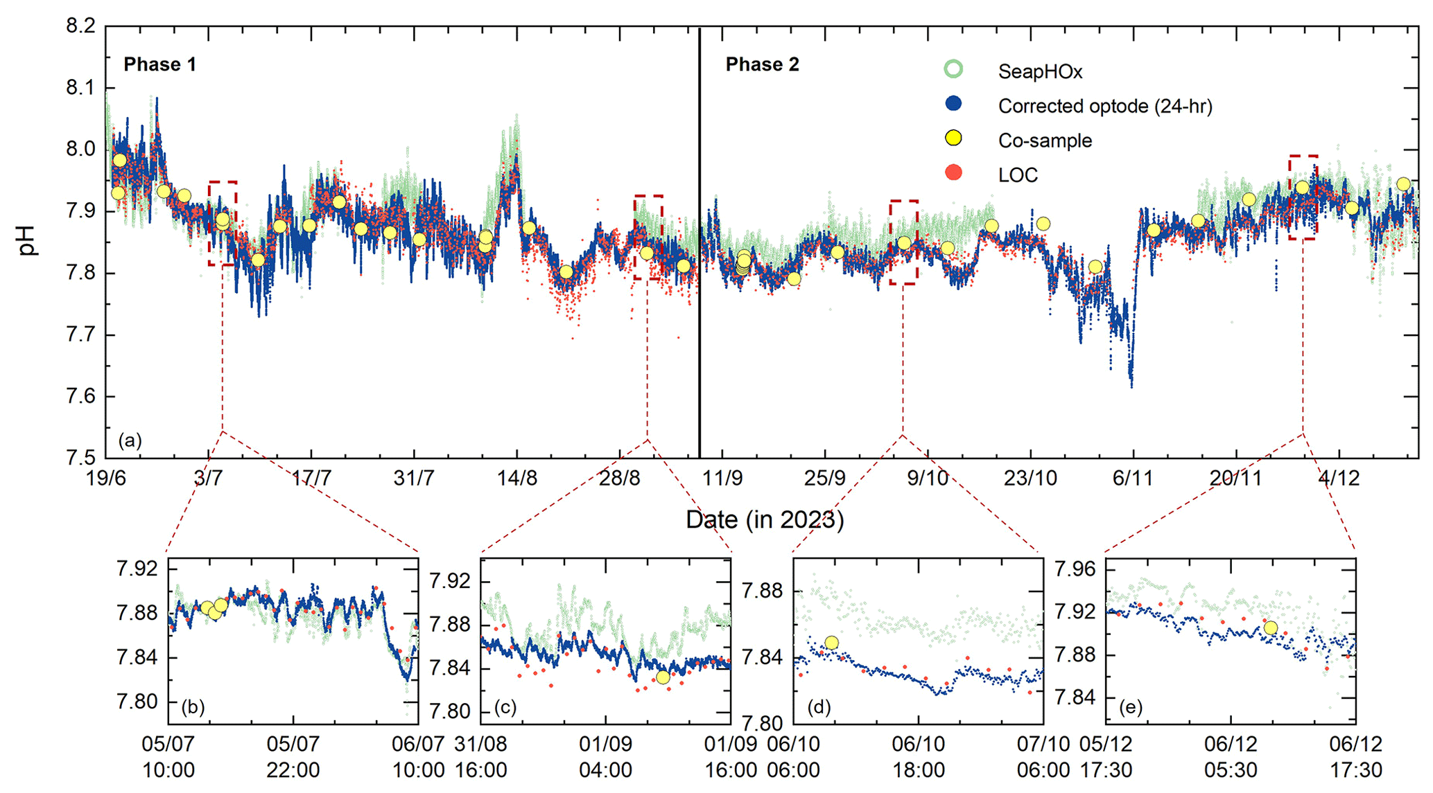
Figure 5 Top panel (a) shows the entire 6-month optode series with 24 h corrected (dark blue filled circles) data with both SeapHOx (sage green unfilled circles) and LOC pH data (red filled circles) overlaid for comparison. Lab validated co-samples are provided for reference (yellow filled circles). Bottom panels (b) through (e) show four zoomed in snapshots within the larger overlaid dataset.

The data plots in the bottom panel of Fig. 5b–e show snapshots of a few exemplar data comparisons between the corrected optode, LOC and SeapHOx sensor data, in addition to lab validated co-samples. At the start of the deployment in late-June (Fig. 5b) we find the corrected optode data and SeapHOx data agreed well with each other (i.e., for this period we calculated a pH difference of +0.003 ± 0.010; 2880 data points in common), are both resolving high-frequency pH fluctuations, and showed good agreement with the three overlaid discrete co-sample data points (i.e., difference of −0.003 for the SeapHOx and a difference of −0.005 for the corrected optode). Around early-September (Fig. 5c) the optode pH values were lower than the SeapHOx pH measurements (i.e., for this period we calculated a pH difference of $-\mathrm{0.024}\pm \mathrm{0.014}$; 2880 data points in common). Nonetheless, both sensors showed relatively good agreement with the discrete co-sample data point (i.e., difference of +0.020 for the SeapHOx and a difference of +0.007 for the corrected optode) despite the significant fouling encountered across the sensors and the fact that at this point the optode sensor was drifting away from the discrete lab-validated samples (refer to Fig. 2). In early-October (Fig. 5d) the offset between the two datasets was still present (i.e., for this period we calculated a pH difference of $-\mathrm{0.028}\pm \mathrm{0.006}$; 287 data points in common), although this is reflective of the LOC pH values used to correct the optode data, which was lower relative to the SeapHOx measurements. A new optode pH cap was installed a month prior to this point, yet it quickly drifted to a relatively constant offset (refer to Fig. 3), but the correction method accounted for this bringing the data in better agreement to the SeapHOx data. The sensors exhibited an offset from the discrete co-sample data point of +0.030 (SeapHOx) and −0.006 (corrected optode). As can be seen the range of pH values was smaller for the optode dataset, which is potentially a result of having a longer response time <60 s (to get 90 % of the signal) due to it being an optical measurement (Wirth et al., 2024; Fritzsche et al., 2018) compared to the SeapHOx response time of ca. 16 s via an electrochemical measurement (Bagshaw et al., 2021). This form of signal smoothing/averaging from optode-based measurements has been noted previously (Fritzsche et al., 2018). As previously mentioned, the manufacturer reported resolution of the optode is 0.003 whereas the SeapHOx has a reported resolution of 0.004. Lastly, in early-December (Fig. 5e) the datasets tracked each other well (i.e., for this period we calculated a pH difference of $-\mathrm{0.012}\pm \mathrm{0.012}$; 287 data points in common) and were in relatively good agreement with the lab validated co-sample (i.e., difference of +0.020 for the SeapHOx and a difference of +0.002 for the corrected optode).

Applying this correction method to our field data, demonstrated that an infrequent, two-point linear correction was sufficient to correct high frequency optode pH data even when compromised by significant signal drifts/offsets. To further support this, Fig. 6 shows the difference (residuals) between the pH measurements from each of the three sensors and the seawater pH obtained from discrete co-samples collected throughout the study. The measurement frequencies for the optode and SeapHOx sensors were sufficiently rapid enough that there was always a measurement taken within ≤1 min of the discrete co-sample collection time. However, due to the lower measurement frequency of the LOC pH sensor, data points collected within ≤30 min were used when comparing LOC data relative to the discrete co-sample data.

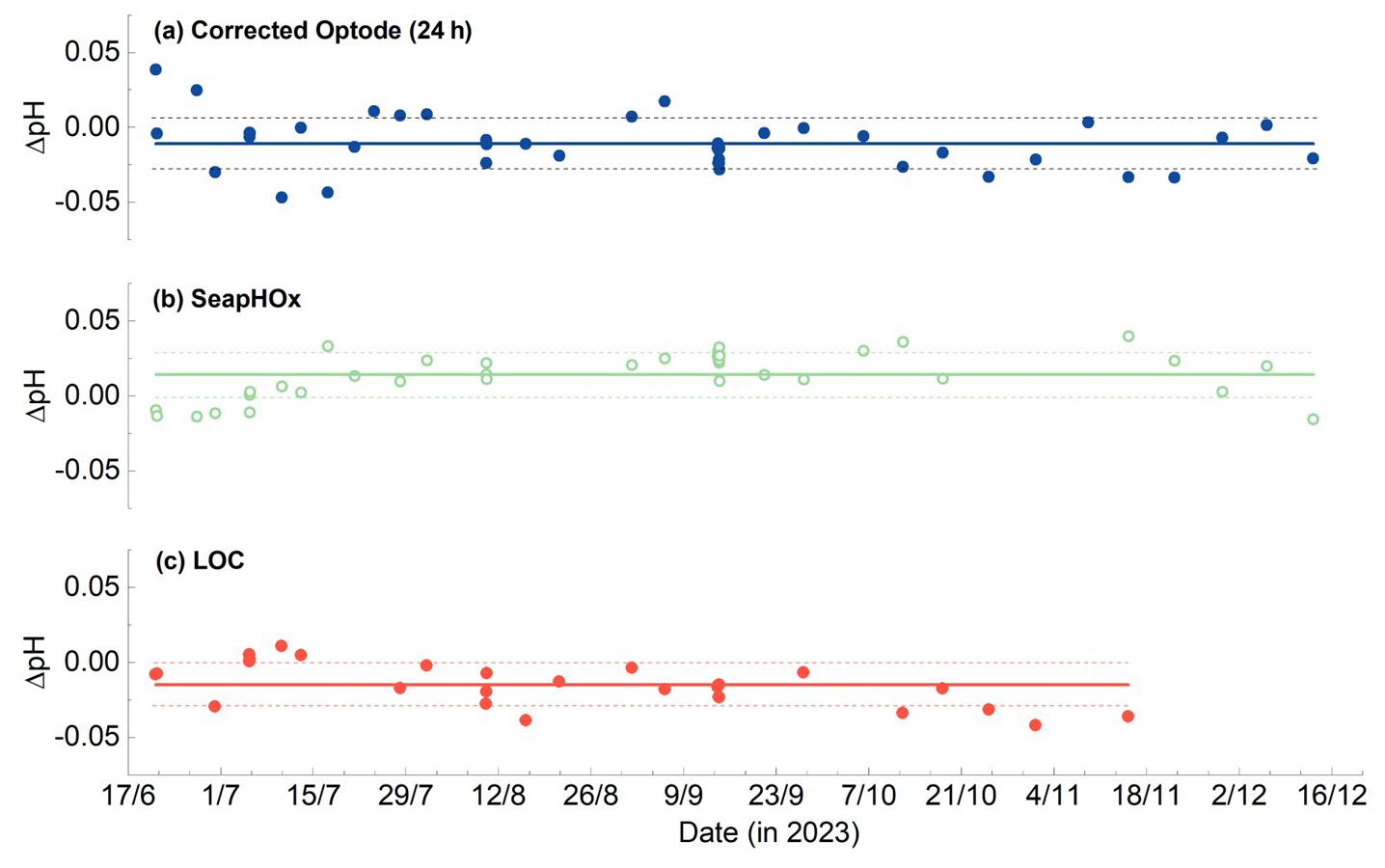
Figure 6 Performance of the three main seawater pH sensor technologies examined as a function of time throughout the deployment. Data are differences (error) relative to discrete lab validated co-samples. The average differences are displayed as solid lines and standard deviations are dashed lines.

The corrected optode data in Fig. 6a collectively suggest a field-obtained performance of $-\mathrm{0.011}\pm \mathrm{0.017}$ (n=44), relative to lab validated co-samples, where the solid line represents the mean error and the dashed lines represent the standard deviation of the error. This performance is comparable to previous reports in the field: +0.027 ± 0.017 (Wirth et al., 2024), $-\mathrm{0.027}\pm \mathrm{0.059}$ (Fritzsche et al., 2018), and others report absolute deviations in the field ranging from 0.019 to 0.051 (Staudinger et al., 2018). Furthermore, when the correction is done with our second LOC dataset (Sect. S5 in the Supplement) the results are similar e.g., a difference of $-\mathrm{0.021}\pm \mathrm{0.025}$ (n=44) is obtained relative to lab validated co-samples. The SeapHOx data (Fig. 6b) appeared at slightly higher pH values relative to the validation samples, and we calculated a difference of +0.014 ± 0.015 (n=38), which is well within the manufacturer reported limits (i.e., ±0.050). The performance of the SeapHOx sensor from our trial was comparable to previous reports in the field utilising ISFET-based pH sensors: <0.025 (Miller et al., 2018), 0.000 ± 0.019 (n=383) (Johnson et al., 2016), +0.007 ± 0.028 (n=26) (Yin et al., 2021), and others report standard deviations between 0.011 and 0.036 (Gonski et al., 2018). The LOC data in Fig. 6c appeared at slightly lower pH values relative to the validation samples, and we calculated a difference of −0.015 ± 0.014 (n=28), which is comparable to +0.003 ± 0.022 (n = 47) with previous work at the same test site (Yin et al., 2021) and other recent fieldwork reporting a difference of +0.001 ± 0.015 (n = 65) between a LOC pH sensor and discrete co-sample data (Nehir et al., 2022). An in-depth comparison of the LOC and SeapHOx pH sensor performance is provided in Sect. S4 in the Supplement. A detailed analysis of the performance of the second optode pH sensor is provided in Sect. S5 in the Supplement. It is worth noting that the SeapHOx pH sensor performance in the field from our work was well within the manufacturer reported limits of ±0.050. Furthermore, the field measured performance of the LOC pH sensor was close to achieving its manufacturer reported performance of <0.009. Therefore, this 6-month shallow water field study has demonstrated that it is feasible to achieve these manufacturer-reported performances.

3.5 Deployment considerations

As previously mentioned, the LOC + optode dual system can provide rapid pH data with low pH offsets (∼ 0.02) relative to validation samples by leveraging low-frequency LOC data to correct drifting/offset high-frequency optode data. To help understand this, a plot of combined sensor performance versus battery charge for a 6-month deployment is provided in Fig. 7, which shows the pH difference relative to lab validated co-samples. Each LOC measurement required ca. 0.15 A (at 12 V) and takes approximately 10 min to complete. Therefore, each measurement used 25 mAh. As can be seen, a correction interval every four weeks (i.e., filled purple circle) substantially improved the pH offset (relative to discrete co-samples) of the raw (uncorrected – filled pink circle) optode pH sensor data, which is approaching the manufacturer reported performance of a SeapHOx-based pH sensor (the dashed red lines indicate ±0.050), and this measurement frequency required only a small amount of power (ca. 150 mAh for 6 months of measurements). The performance can be further improved by taking a LOC measurement once per week (e.g., filled green circle) and requires ca. 600 mAh for 6 months of operation. The improvements in performance largely plateau after this correction interval. Beyond this, more frequent measurements did not give significant enhancements (relative to discrete samples) in comparison to the charge required. For example, the filled black circle (Fig. 7) represents a 1 d correction interval and requires ca. 4500 mAh whereas the filled blue circle represents a correction every 1 h and requires 107 600 mAh for 6 months. Overall, we find that a single in-situ LOC measurement every 1–7 d is sufficient to provide minimal offsets (∼ 0.02 relative to validation samples) and rapid pH data with this combined sensor package. Operating the LOC pH sensor at these low measurement frequencies is advantageous as it reduces reagent consumption, waste generation and power consumption, which taken together would also lower the sensor service intervals. This will, however, still be dictated by the specific deployment conditions and requirements.

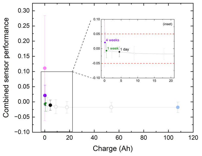
Figure 7 Plot of combined LOC-optode sensor package performance (relative to lab validation samples) as a function of charge required (by the LOC). The colour- filled circle symbols are highlighted to illustrate five distinct points (i.e., uncorrected, 1 month, 1 week, 1 d, and 1 h correction intervals). An inset provides a clearer zoomed-in region, and the dashed red lines indicate ±0.05 for visual purposes.

The above demonstrates that the optode sensor was markedly improved to provide comparable performance to a SeapHOx sensor (i.e., ∼ 0.02) by means of a simple and infrequent in-situ correction. Using the combined pH sensor package showcased here, the operator can select the LOC sensor measurement frequency needed to correct optode data for a particular application. If more charge is available, then a more frequent correction interval can be used or equally this can be reduced to conserve charge with a known impact on performance. A commercial deep-sea rated battery the physical size of the LOC sensor itself can provide 50 Ah of charge (https://subctech.com/ocean-power/basic-batteries/, last access: 29 August 2025), which is sufficient to power the LOC pH sensor for a 6-month deployment measuring every 3 h. Furthermore, the small form-factor of the optode pH sensor is advantageous for incorporation onto a range of autonomous vehicles. In fact, the optode pH sensor is small enough to fit inside the standard reagent housing of the LOC pH sensor itself. The LOC + optode sensor system provided complementary strengths of low/stable pH offsets (LOC) and rapid (optode) data collection. Furthermore, having two sensor technologies enhances data robustness, provides flexibility in expanding modular observational networks, and removes the reliance on a single commercial platform that can be vulnerable to supply/servicing issues. For a long-term (>6 months) deployment, the low measurement frequencies from the LOC pH sensor needed to correct optode data required small reagent volumes (e.g., ∼ 40 µL of reagent consumed and ∼ 25 mL total waste volume if sampling once every 4 weeks over a 1-year deployment) thus permitting space to incorporate the optode within the standard reagent housing. Future work will look at developing an integration protocol for this combined sensor package and establish communication procedures that could allow this data correction to be done in-situ.

4 Conclusions

Overall, this work has demonstrated a combined pH sensor system capable of providing comparable performance (i.e., ∼ 0.02) to an independent reference pH sensor, rapid (<1 min measurement⁻¹), and long-term (6-month) seawater pH data. This was accomplished by leveraging pH data obtained from a LOC pH sensor measuring at low frequencies to correct signal drift/offset from an optode-based pH sensor measuring at a very high frequency. During a six-month shallow water deployment in a high biofouling environment, we observed significant signal drift and offsets in the optode pH sensor, whereas the LOC and SeapHOx sensors returned comparable performances (∼ 0.02) relative to discrete co-samples. To improve the optode data, a linear rate correction method was demonstrated, and we found that even if the LOC sensor had sampled with measurement frequencies of several days to several weeks, it was sufficient to significantly improve the performance of the high-frequency optode data (e.g., a LOC data point once every week gave a difference of $-\mathrm{0.007}\pm \mathrm{0.024}$ (n=44) relative to lab validated co-samples for the corrected optode dataset). More frequent corrections improved performance but only slightly (i.e., the performance approached that of the LOC sensor used to correct the optode data). For deployment on long-term platforms such as moorings, an optimum balance can be identified between performance and battery capacity for the intended deployment. The corrected optode measurements achieved RMSE values on the order of ∼ 0.02 relative to discrete co-samples, thus meeting the GOA-ON weather-quality observational target, which is sufficient for resolving short-term variability in coastal carbonate chemistry while minimising reagent consumption and operational complexity.