Analytical approaches for wave energy dissipation induced by wave-generated turbulence and random wave-breaking

This paper is dedicated to investigate the dissipation effects of wave-generated turbulence reacting on ocean waves and to estimate the energy loss due to wave-breaking theoretically. An analytical dissipation source function induced by wave-generated turbulence in the water was proposed through the equilibrium solutions of a second-order turbulence closure model between the wave shear instability generations and the turbulent kinetic energy (TKE) dissipations under the well-founded structural equilibrium closure assumptions. And an improved postbreaking spectrum expression, based on the breaking wave statistical method, was presented to depict more explicitly the intermittent wave-breaking events. Comparisons of the TKE dissipation rates indicate that the model results agree well with the laboratory observations which were directly generated by the waves themselves, but for mechanical and wind waves, dispersions suggest the presence of other dynamic processes. The modeled attenuation coefficients of the breaking spectrum correspond to the decreasing tendency measured from the lake experiment, which yields valuable insights of the physics of dominant breaking, but the statistical approach is less well-suited for simulating the rapid transient regime of wave breaking as well as for the higher frequency in the equilibrium range. Evaluations for more complex situations will be addressed in the future series of papers.

1 Introduction

The third generation ocean wave models, which integrate the dynamical equations that describe the evolution of a wave field, have been widely used in scientific studies and practical applications. Though input mechanisms, in particular bulk transfer of energy action and momentum to waves, and other source terms are not well established either, the least understood aspect of the physics of wave model is the dissipation terms (Donelan and Yuan, 1994; Young and Babanin, 2006; Babanin, 2011). The dissipation source (sink) terms induced by wave-generated turbulence and random wave-breaking are the subject of the present paper. There are a number of dissipation mechanisms studied previously through either experimental or analytical (or both) approaches, and they have advanced very significantly over the past decades. However, there remains a notable gap in mechanism research pertaining to varied parameterizations and applications in wave models.

Concerning to the wave-breaking dissipation, the most mathematically well-advanced and most frequently utilized whitecap model is that of Hasselmann (1974) which involves the whitecaps are weak-in-the-mean and the dissipation is a linear function of the spectrum, and its parameterization has been proposed and further extended in various WAM-Cycle models by Komen et al. (1984), WAMDI G. (1988), Bidlot et al. (2005), Bidlot (2012), etc. Following the quasi-saturated ideas of Phillips (1985) and numerical modeling framework of Alves and Banner (2003), Ardhuin et al. (2009b, 2010), Filipot and Ardhuin (2012) presented an improved wave-breaking dissipation parameterization as the sum of the saturation-based term and a cumulative breaking term, while the latter represents the smoothing of the surface by big breakers that wipe out smaller waves. The probability model due to wave breaking was proposed by Longuet-Higgins (1969), Yuan et al. (1986) and Hua and Yuan (1992). This kind of wave-breaking dissipation source function was derived from the breaking wave statistics, in which the power of the normalized integral wave steepness parameter is $\mathrm{1}/\mathrm{2}$ and less than that of whitecap model. So the probability model gives lower dissipation value for the high sea state condition (Yuan et al., 1993), and has been applied in the LAGFD (Laboratory of Geophysical Fluid Dynamics)-WAM wave model and MASNUM (Key Laboratory of MArine Science and NUmerical Modeling) wave model (Yuan et al., 1991; Yang et al., 2005). Though conceptually attractive, its practical parameterization fitted to the whitecap model is deprived of its own discretionary estimates of the dissipation rate. Based on the random phase spectral action density balance equation for wavenumber-direction spectra and evolved from earlier WW1 and WW2 (WAVEWATCH I & II) model packages (Tolman, 1991, 1992), the comprehensive source terms were incorporated and employed in WW3 ((WAVEWATCH III) wave model by Tolman and Chalikov (1996), Chalikov and Belevich (1993), Chalikov (1995) , Tolman (2002), etc. Young and Babanin (2006) summarized series of previous experimental attempts to obtain an experimental spectral dissipation function, and based on direct estimates of wave energy loss due to dominant breaking through their comprehensive measurement records at Lake George, they proposed a new spectral dissipation source term due to wave breaking. This experimental parameterization was improved and employed in WW3 (WAVEWATCH III) wave model (Babanin et al., 2007, 2010; Babanin, 2009; Rogers et al., 2012; Liu et al., 2019; WW3DG, 2019). The quantitative match is dubious between the latter applications and the former experimental estimates, despite only a single field record was analyzed but verified approximately by turbulent kinetic energy (TKE) dissipation rates which were retrieved from synchronously ADV measured turbulence spectra (Young and Babanin, 2006). In addition, the physical meaning of wave-breaking dissipation rate (time derivative of wave energy spectrum), as stated in previous studies, remains fuzzy and vague because the wave-breaking process is not continuous but very short and intermittent, which stimulate us to propose an improved analytical postbreaking spectrum expression, from the point of view of the probability theory, for practical implementation. This constitutes one of our primary focal points of this study.

Polnikov (1994, 2005, 2010) and Polnikov and Tkalich (2006) argued that the mechanism of wave energy dissipation is completely conditioned by the interaction between wave motions and the turbulence of the upper water layer, and the latter is generated by a great number of physical processes, including different kinds of hydrodynamic instabilities of mechanical motions near the interface. They solved Reynolds' equation where the Reynolds' stress was expanded into a series with respect to velocity components and their spatial derivatives. The Prandtl mixing-length hypothesis was used to close the turbulent terms in these series. Their physical treatment is attractive, but the theory needs further development (Young and Babanin, 2006), even though it was further constructed by means of the phenomenological similarity method and spectrally justified in the frame of the proposed eddy viscosity model (Polnikov, 2012). Tolman and Chalikov (1996) also suggested a turbulent dissipation analogy for tunable closure modeling. For dominant low-frequency dissipation, if wave motion and turbulence are not correlated, their interaction can be accounted for by introducing an effective, although weak, turbulent viscosity coefficient in the oceanic boundary layer. But for poorly understood high-frequency dissipation, a diagnostic high-frequency dissipation was defined and designed to result in a consistent source term balance. And the total dissipation source term was defined as a linear combination of the above high and low frequency constituents. Their separation parameterization for the dissipation term is physically meaningful and the heuristic arguments have been employed in WW3 ST2 package and widely applied in many practical numerical models. In fact, during the past two decades, a series of studies concerned with mechanisms of nonbreaking wave-generated turbulence and its mixing effects on upper ocean layers have been achieved significantly and their conclusions have been confirmed more exhaustively by experiments. The theoretical wave-generated turbulence theory can be established by two different but relatively consistent approaches: the first approach involves the use of a parameterization form similar to the classical Prandtl mixing-length theory, and the second approach involves the use of the equilibrium solutions of a high-deterministic second-order turbulence closure model between the wave motion shear instability generations and the TKE dissipations (Baumert et al., 2005), then the analytical mixing coefficients were proposed to elaborate the dominant mixing intensity induced by wave-generated turbulence in the upper ocean (Yuan et al., 1999; Yuan et al., 2013). Qualitative and quantitative validations by field measurements and improvements of wave-current coupled modelling indicate the key mixing role in the formation of upper mixed layers (Qiao et al., 2004, 2010; Xia et al., 2004, 2006; Shu et al., 2011; Shi et al., 2016, 2019; Yu et al., 2020; Zhuang et al., 2020, 2021, 2022; Yang et al., 2003, 2004, 2019, 2022). But how the reaction of wave-generated turbulence on ocean waves was disregarded in their studies, which is still lack and needs to investigate further. Babanin (2006), Babanin and Haus (2009), Dai et al. (2010) tested and confirmed the nonbreaking wave-generated turbulence through mechanically generated laboratory wave experiments. Babanin and Chalikov (2012) also presented that the vorticity and turbulence usually occur in vicinity of wave crests and then spread over upwind slope and downward through a numerical wave-turbulence model. Based on their experimental approximations, a parameterization of swell dissipation rate was proposed, verified through altimeter observation data and employed in WW3 ST6 package (Babanin, 2011, 2012; Young et al., 2013; Zieger et al., 2015; WW3DG, 2019). In fact, an analytical parameterization for wave energy dissipation can be effectively deduced through the equilibrium solutions of wave-generated turbulence, which will be described in detail and implemented in numerical experiments below. It constitutes the other focal point of this study to illustrate the important role of dissipation induced by wave-generated turbulence, which is definitely the feedback of imparting of wave shear instability generations on turbulence.

There are also a number of other dissipation mechanisms which are certainly not negligible in the wave system. Prominent negative input source term for swell was introduced by Chalikov and Belevich (1993), Chalikov (1995), Tolman and Chalikov (1996), Tolman (2002) and Chalikov and Babanin (2019) where the phase velocity of waves is larger than the wind velocity, which means that the dynamic pressure of the wind on the forward face of the wave component exceeds the pressure on the backward face and waves accelerate wind, resulting in the momentum and energy fluxes from the waves to the wind. Based on the direct measurements of turbulent air-sea fluxes obtained during several sea expeditions, Grachev and Fairall (2001) verified that long ocean waves (swell) traveling faster than local wind and in the same direction cause upward momentum transport, implying a negative drag coefficient. A weak damping of swells was also introduced by Janssen (2004), who proposed an asymptotic linearization of the small effects of air turbulent eddies. Ardhuin et al. (2009a, 2010), Collard et al. (2009) proposed a nonlinear swell dissipation parameterization, which is related to a laminar-to-turbulent transition of the oscillatory boundary layer over swells, using the spaceborne SAR observed swell fields from the European Space Agency's (ESA) ENVISAT satellite. Interaction of ocean waves and upper ocean turbulence, while the latter is induced by Stokes drift shears, accounts for a significant fraction of the energy losses of the wave field (McWilliams et al., 1997; Teixeira and Belcher, 2002; Ardhuin and Jenkins, 2006; Guo and Shen, 2013, 2014). Evaluations indicated it is much weaker than other dissipations (Ardhuin et al., 2010), despite this its formula is employed in WW3 ST4 package. Model results showed that its effects significantly improve simulations of turbulence characteristics and upper ocean thermal structure (Huang and Qiao, 2010; Huang et al., 2011). Sea bottom-wave interactions and ice-wave interactions have been studied in great detail, which are out of scope of present study and not discussed here.

The objectives of this paper are to explore the dissipation effects of wave-generated turbulence reacting on ocean waves, and to investigate the role of wave-breaking dissipation via an improved postbreaking spectrum expression based on the breaking wave statistical method. The remainder of this paper is organized as follows: Sect. 2 describes the analytical approaches for wave energy dissipation induced by wave-generated turbulence and by random wave-breaking, introduces scale detection comparing to wind input and provides verifications with laboratory observations or comprehensive measurements; Sect. 3 presents application implementations on simple duration-limited growth and decay experiments; Sect. 4 addresses discussions and issues which need complex insights, and some conclusions and suggestions for future research are summarized in Sect. 5.

2 Model derivation and verification

2.1 The analytical approach for wave energy dissipation induced by wave-generated turbulence

In the usual notation, let $x_i,i=\mathrm{1},\mathrm{2},\mathrm{3}$ be rectangular co-ordinates (The list of symbols is provided in Appendix D). Let $u_{\mathrm{SM}i},i=\mathrm{1},\mathrm{2},\mathrm{3}$ denote the wave velocities; $T_{\mathrm{SM}},s_{\mathrm{SM}},p_{\mathrm{SM}},{\mathit{\rho }}_{\mathrm{SM}}$ the perturbations of temperature, salinity, pressure and density induced by ocean waves. More comprehensive governing equations for wave motion were derived in Yuan et al. (2012) and Yang et al. (2022) under the assumption that turbulence timescale is much shorter than wave period, and the unit volume wave energy balance equation can be obtained in tensor expression as follows (see Appendix A):

$$\begin{array}{}\text{(1)}& \begin{array}{l}\frac{\partial }{\partial t}{〈\frac{{\mathit{\rho }}_{\mathrm{0}}{u}_{\mathrm{SM}i}^{\mathrm{2}}}{\mathrm{2}}+\frac{g^{\mathrm{2}}{\mathit{\rho }}_{\mathrm{SM}}^{\mathrm{2}}}{\mathrm{2}{\mathit{\rho }}_{\mathrm{0}}{\widehat{N}}_{\mathrm{3}}^{\mathrm{2}}}〉}_{\mathrm{SM}}+{〈\left({\widehat{U}}_j+u_{\mathrm{SM}j}\right)\frac{\partial }{\partial x_j}\left(\frac{{\mathit{\rho }}_{\mathrm{0}}{u}_{\mathrm{SM}i}^{\mathrm{2}}}{\mathrm{2}}+\frac{g^{\mathrm{2}}{\mathit{\rho }}_{\mathrm{SM}}^{\mathrm{2}}}{\mathrm{2}{\mathit{\rho }}_{\mathrm{0}}{\widehat{N}}_{\mathrm{3}}^{\mathrm{2}}}\right)〉}_{\mathrm{SM}}+\frac{\partial }{\partial x_i}{〈p_{\mathrm{SM}}{u}_{\mathrm{SM}i}〉}_{\mathrm{SM}}\\ =\left(-{\mathit{\rho }}_{\mathrm{0}}{〈u_{\mathrm{SM}i}{u}_{\mathrm{SM}j}〉}_{\mathrm{SM}}\frac{\partial {\widehat{U}}_i}{\partial x_j}+g{〈{\mathit{\rho }}_{\mathrm{SM}}{u}_{\mathrm{SM}\mathit{\alpha }}〉}_{\mathrm{SM}}\frac{{\widehat{N}}_{\mathit{\alpha }}^{\mathrm{2}}}{{\widehat{N}}_{\mathrm{3}}^{\mathrm{2}}}\right)+\frac{g^{\mathrm{2}}}{{\mathit{\rho }}_{\mathrm{0}}{\widehat{N}}_{\mathrm{3}}^{\mathrm{2}}}{〈{\mathit{\rho }}_{\mathrm{SM}}{Q}_{{\mathit{\rho }}_{\mathrm{SM}}}〉}_{\mathrm{SM}}\\ +\left\{\begin{array}{l}\frac{\partial }{\partial x_j}{〈\left({\mathit{\nu }}_{\mathrm{0}}+\frac{k^{\mathrm{2}}}{{\mathit{\pi }}^{\mathrm{2}}\mathit{\epsilon }}\right)\frac{\partial }{\partial x_j}\left(\frac{{\mathit{\rho }}_{\mathrm{0}}{u}_{\mathrm{SM}i}^{\mathrm{2}}}{\mathrm{2}}\right)〉}_{\mathrm{SM}}+\frac{\partial }{\partial x_j}{〈\left(K_{\mathrm{0}}+\frac{\mathrm{1}}{{\mathit{\sigma }}_{\mathrm{0}}}\frac{k^{\mathrm{2}}}{{\mathit{\pi }}^{\mathrm{2}}\mathit{\epsilon }}\right)\frac{\partial }{\partial x_j}\left(\frac{g^{\mathrm{2}}{\mathit{\rho }}_{\mathrm{SM}}^{\mathrm{2}}}{\mathrm{2}{\mathit{\rho }}_{\mathrm{0}}{\widehat{N}}_{\mathrm{3}}^{\mathrm{2}}}\right)〉}_{\mathrm{SM}}\\ -{〈{\mathit{\rho }}_{\mathrm{0}}\left({\mathit{\nu }}_{\mathrm{0}}+\frac{k^{\mathrm{2}}}{{\mathit{\pi }}^{\mathrm{2}}\mathit{\epsilon }}\right){\left(\frac{\partial u_{\mathrm{SM}i}}{\partial x_j}\right)}^{\mathrm{2}}〉}_{\mathrm{SM}}-{〈\frac{g^{\mathrm{2}}}{{\mathit{\rho }}_{\mathrm{0}}{\widehat{N}}_{\mathrm{3}}^{\mathrm{2}}}\left(K_{\mathrm{0}}+\frac{\mathrm{1}}{{\mathit{\sigma }}_{\mathrm{0}}}\frac{k^{\mathrm{2}}}{{\mathit{\pi }}^{\mathrm{2}}\mathit{\epsilon }}\right){\left(\frac{\partial {\mathit{\rho }}_{\mathrm{SM}}}{\partial x_j}\right)}^{\mathrm{2}}〉}_{\mathrm{SM}}\end{array}\right\}\end{array}\end{array}$$

where ${\widehat{U}}_i,i=\mathrm{1},\mathrm{2},\mathrm{3};\widehat{T},\widehat{s},\widehat{p},\widehat{\mathit{\rho }}$ denote the background current components and ρ₀ is the basin mean water density; ${\mathit{\nu }}_{\mathrm{0}},K_{\mathrm{0}},D_{\mathrm{0}}$ the molecular viscosity, thermal and diffusion coefficients; ${\widehat{N}}_i^{\mathrm{2}}=-g\frac{\partial }{\partial x_i}\left(\frac{\widehat{\mathit{\rho }}}{{\mathit{\rho }}_{\mathrm{0}}}\right),i=\mathrm{1},\mathrm{2},\mathrm{3}$ the Brunt–Väisälä frequency components; ${\mathit{\sigma }}_{\mathrm{0}}=\frac{\mathrm{1}}{\mathrm{2}}$ the Prandtl number; k,ε the kinetic energy and its dissipation rate of ocean turbulence, which is generated by shear instability of background current (Mellor and Yamada, 1982), Stokes drift (Ardhuin and Jenkins, 2006; Ardhuin et al., 2010; Huang and Qiao, 2010) but mainly generated by ocean waves in the upper layers (Yuan et al., 1999, 2013; Qiao et al., 2004; Yang et al. , 2003, 2004; Babanin, 2006; Babanin and Haus, 2009; Dai et al., 2010; Zhuang et al., 2022). $\frac{{\mathit{\rho }}_{\mathrm{0}}{u}_{\mathrm{SM}i}^{\mathrm{2}}}{\mathrm{2}},\frac{g^{\mathrm{2}}{\mathit{\rho }}_{\mathrm{SM}}^{\mathrm{2}}}{\mathrm{2}{\mathit{\rho }}_{\mathrm{0}}{\widehat{N}}_{\mathrm{3}}^{\mathrm{2}}}$ denote the kinetic and potential wave energy and 〈⋅〉_SM denotes the Reynolds average on the wave motion. Hereafter, other symbols have their usual meaning. The first term on the left-hand side of Eq. (1) is related to the local mechanical energy variation and the second and third ones denote the energy flux transferred by ocean waves and background currents. The first and second terms on the right-hand side of Eq. (1) are related to the modulation by larger scale motions through shear instability generations. The third term is related to the energy input through thermal radiation, the fourth and fifth ones are related to the modulation by smaller scale motions through ocean mixing and the last two terms are related to the energy loss rate due to internal viscosity. It should be noted that three types of gravity ocean waves, which consist of surface waves, internal waves and inertial waves, follow the same governing Eq. (1). Here in this study only the former is concerned, so the fifth term on the right-hand side of Eq. (1) is the energy dissipation induced by ocean turbulence (Dissipation induced by molecular viscosity is insignificant and not considered here).

As stated above, ocean wave-generated turbulence plays a dominant role in the upper layers, the energy loss from ocean waves needs to be studied further. The unit volume energy dissipation mainly induced by wave-generated turbulence can be expressed as

$$\begin{array}{}\text{(2)}& -{〈{\mathit{\rho }}_{\mathrm{0}}{\displaystyle \frac{k^{\mathrm{2}}}{{\mathit{\pi }}^{\mathrm{2}}\mathit{\epsilon }}}{\left({\displaystyle \frac{\partial u_{\mathrm{SM}i}}{\partial x_j}}\right)}^{\mathrm{2}}〉}_{\mathrm{SM}}=-{\mathit{\rho }}_{\mathrm{0}}{\mathit{\alpha }}_{\mathrm{wt}}{〈{\displaystyle \frac{{\stackrel{\mathrm{‾}}{k}}^{\mathrm{2}}}{{\mathit{\pi }}^{\mathrm{2}}\stackrel{\mathrm{‾}}{\mathit{\epsilon }}}}〉}_{\mathrm{SM}}{〈{\left({\displaystyle \frac{\partial u_{\mathrm{SM}i}}{\partial x_j}}\right)}^{\mathrm{2}}〉}_{\mathrm{SM}}\end{array}$$

where the symbol overbar “−” denotes the turbulent equilibrium variables, ${〈\frac{{\stackrel{\mathrm{‾}}{k}}^{\mathrm{2}}}{{\mathit{\pi }}^{\mathrm{2}}\stackrel{\mathrm{‾}}{\mathit{\epsilon }}}〉}_{\mathrm{SM}}$ is the so-called wave-generated turbulent mixing coefficient which was widely used in coupling numerical models. α_wt is an undetermined constant here, which implies the quasi-equilibrium level of wave-generated turbulence. Then the total energy dissipation for vertical water column per unit area can be written as

$$\begin{array}{}\text{(3)}& \begin{array}{rl}& -\underset{-\widehat{H}}{\overset{\mathrm{0}}{\int }}{〈{\mathit{\rho }}_{\mathrm{0}}{\displaystyle \frac{k^{\mathrm{2}}}{{\mathit{\pi }}^{\mathrm{2}}\mathit{\epsilon }}}{\left({\displaystyle \frac{\partial u_{\mathrm{SM}i}}{\partial x_j}}\right)}^{\mathrm{2}}〉}_{\mathrm{SM}}\mathrm{d}{x}_{\mathrm{3}}\\ & =-{\mathit{\rho }}_{\mathrm{0}}{\mathit{\alpha }}_{\mathrm{wt}}\underset{-\widehat{H}}{\overset{\mathrm{0}}{\int }}{〈{\displaystyle \frac{{\stackrel{\mathrm{‾}}{k}}^{\mathrm{2}}}{{\mathit{\pi }}^{\mathrm{2}}\stackrel{\mathrm{‾}}{\mathit{\epsilon }}}}〉}_{\mathrm{SM}}{〈{\left({\displaystyle \frac{\partial u_{\mathrm{SM}i}}{\partial x_j}}\right)}^{\mathrm{2}}〉}_{\mathrm{SM}}\mathrm{d}{x}_{\mathrm{3}}\end{array}\end{array}$$

where $\widehat{H}$ denotes the water depth.

In the statistical wave theory, the wave field is regarded as weakly-in-the-mean nonlinear processes and the chief linear components are used widely for further detection (Komen et al., 1994). Below we try to derive the total energy dissipation expressed by wavenumber spectrum through the classical linear wave solutions, i.e.,

$$\begin{array}{}\text{(4)}& {\displaystyle }{u}_{\mathrm{SM}\mathrm{1}}=\int \underset{\mathit{k}}{\int }{\displaystyle \frac{\mathit{\omega }{k}_{\mathrm{1}}}{K}}A{\displaystyle \frac{\cosh K(\widehat{H}+x_{\mathrm{3}})}{\sinh K\widehat{H}}}\exp \left\{i\left(\mathit{k}\cdot \mathit{r}-\mathit{\omega }t\right)\right\}\mathrm{d}\mathit{k}\text{(5)}& {\displaystyle }{u}_{\mathrm{SM}\mathrm{2}}=\int \underset{\mathit{k}}{\int }{\displaystyle \frac{\mathit{\omega }{k}_{\mathrm{2}}}{K}}A{\displaystyle \frac{\cosh K(\widehat{H}+x_{\mathrm{3}})}{\sinh K\widehat{H}}}\exp \left\{i\left(\mathit{k}\cdot \mathit{r}-\mathit{\omega }t\right)\right\}\mathrm{d}\mathit{k}\text{(6)}& {\displaystyle }{u}_{\mathrm{SM}\mathrm{3}}=\int \underset{\mathit{k}}{\int }-\mathit{\omega }iA{\displaystyle \frac{\sinh K(\widehat{H}+x_{\mathrm{3}})}{\sinh K\widehat{H}}}\exp \left\{i\left(\mathit{k}\cdot \mathit{r}-\mathit{\omega }t\right)\right\}\mathrm{d}\mathit{k}\end{array}$$

where the wavenumber vector $\mathit{k}=\left(k_{\mathrm{1}},k_{\mathrm{2}}\right)$ with $K=\sqrt{k_{\mathrm{1}}^{\mathrm{2}}+k_{\mathrm{2}}^{\mathrm{2}}}$, $\mathit{r}=\left(x_{\mathrm{1}},x_{\mathrm{2}}\right)$. ω denotes the radian frequency, and A, the wave amplitude.

For a spatially homogeneous and temporally stationary wave field, the product ${〈\frac{\partial u_{\mathrm{SM}\mathrm{1}}}{\partial x_{\mathrm{1}}}\frac{\partial u_{\mathrm{SM}\mathrm{1}}}{\partial x_{\mathrm{1}}}〉}_{\mathrm{SM}}$ is simplified as

$$\begin{array}{}\text{(7)}& \begin{array}{l}{〈\frac{\partial u_{\mathrm{SM}\mathrm{1}}}{\partial x_{\mathrm{1}}}\frac{\partial u_{\mathrm{SM}\mathrm{1}}}{\partial x_{\mathrm{1}}}〉}_{\mathrm{SM}}=\\ \int \underset{\mathit{k}}{\int }Re\left\{\begin{array}{l}\int \underset{{\mathit{k}}^{\prime }}{\int }\mathit{\omega }{\mathit{\omega }}^{\prime }\frac{k_{\mathrm{1}}^{\mathrm{2}}}{K}\frac{k_{\mathrm{1}}^{{}^{\prime }\mathrm{2}}}{K^{\prime }}\frac{\cosh K(\widehat{H}+x_{\mathrm{3}})}{\sinh K\widehat{H}}\frac{\cosh K^{\prime }(\widehat{H}+x_{\mathrm{3}})}{\sinh K^{\prime }\widehat{H}}\\ 〈A{A}^{*}\exp \left\{i\left[(k_{\mathit{\alpha }}-k_{\mathit{\alpha }}^{\prime })x_{\mathit{\alpha }}-(\mathit{\omega }-{\mathit{\omega }}^{\prime })t\right]\right\}〉\mathrm{d}{k}_{\mathrm{1}}^{\prime }\mathrm{d}{k}_{\mathrm{2}}^{\prime }\end{array}\right\}\mathrm{d}{k}_{\mathrm{1}}\mathrm{d}{k}_{\mathrm{2}}\\ =\int \underset{\mathit{k}}{\int }Re\left\{\begin{array}{l}\int \underset{{\mathit{k}}^{\prime }}{\int }\mathit{\omega }{\mathit{\omega }}^{\prime }\frac{k_{\mathrm{1}}^{\mathrm{2}}}{K}\frac{k_{\mathrm{1}}^{{}^{\prime }\mathrm{2}}}{K^{\prime }}\frac{\cosh K(\widehat{H}+x_{\mathrm{3}})}{\sinh K\widehat{H}}\frac{\cosh K^{\prime }(\widehat{H}+x_{\mathrm{3}})}{\sinh K^{\prime }\widehat{H}}\\ \mathit{\delta }(\mathit{k}-{\mathit{k}}^{\prime })E(k_{\mathrm{1}},k_{\mathrm{2}})\mathrm{d}{k}_{\mathrm{1}}^{\prime }\mathrm{d}{k}_{\mathrm{2}}^{\prime }\end{array}\right\}\mathrm{d}{k}_{\mathrm{1}}\mathrm{d}{k}_{\mathrm{2}}\\ =\int \underset{\mathit{k}}{\int }{\mathit{\omega }}^{\mathrm{2}}\frac{k_{\mathrm{1}}^{\mathrm{4}}}{K^{\mathrm{2}}}\frac{{\cosh }^{\mathrm{2}}K(\widehat{H}+x_{\mathrm{3}})}{{\sinh }^{\mathrm{2}}K\widehat{H}}E(k_{\mathrm{1}},k_{\mathrm{2}})\mathrm{d}{k}_{\mathrm{1}}\mathrm{d}{k}_{\mathrm{2}}\end{array}\end{array}$$

where δ(⋅) denotes the Dirac function and E(k₁,k₂), the wavenumber spectrum (Kinsman, 2012).

Correspondingly, after some similar manipulations and summing over all product terms, we obtain

$$\begin{array}{}\text{(8)}& \begin{array}{rl}{〈{\displaystyle \frac{\partial u_{\mathrm{SM}i}}{\partial x_j}}{\displaystyle \frac{\partial u_{\mathrm{SM}i}}{\partial x_j}}〉}_{\mathrm{SM}}& =\int \underset{\mathit{k}}{\int }\mathrm{2}{\mathit{\omega }}^{\mathrm{2}}{K}^{\mathrm{2}}{\displaystyle \frac{\cosh \mathrm{2}K(\widehat{H}+x_{\mathrm{3}})}{{\sinh }^{\mathrm{2}}K\widehat{H}}}\\ & E(k_{\mathrm{1}},k_{\mathrm{2}})\mathrm{d}{k}_{\mathrm{1}}\mathrm{d}{k}_{\mathrm{2}}\end{array}\end{array}$$

Hence,

$$\begin{array}{}\text{(9)}& \begin{array}{l}-\underset{-\widehat{H}}{\overset{\mathrm{0}}{\int }}{〈{\mathit{\rho }}_{\mathrm{0}}\frac{k^{\mathrm{2}}}{{\mathit{\pi }}^{\mathrm{2}}\mathit{\epsilon }}{\left(\frac{\partial u_{\mathrm{SM}i}}{\partial x_j}\right)}^{\mathrm{2}}〉}_{\mathrm{SM}}\mathrm{d}{x}_{\mathrm{3}}=-{\mathit{\rho }}_{\mathrm{0}}g\int \underset{\mathit{k}}{\int }\mathrm{2}{\mathit{\alpha }}_{\mathrm{wt}}\frac{{\mathit{\omega }}^{\mathrm{2}}{K}^{\mathrm{2}}}{g}\\ \left[\underset{-\widehat{H}}{\overset{\mathrm{0}}{\int }}{〈\frac{{\stackrel{\mathrm{‾}}{k}}^{\mathrm{2}}}{{\mathit{\pi }}^{\mathrm{2}}\stackrel{\mathrm{‾}}{\mathit{\epsilon }}}〉}_{\mathrm{SM}}\frac{\cosh \mathrm{2}K(\widehat{H}+x_{\mathrm{3}})}{{\sinh }^{\mathrm{2}}K\widehat{H}}\mathrm{d}{x}_{\mathrm{3}}\right]E(k_{\mathrm{1}},k_{\mathrm{2}})\mathrm{d}{k}_{\mathrm{1}}\mathrm{d}{k}_{\mathrm{2}}\\ =-{\mathit{\rho }}_{\mathrm{0}}g\int \underset{\mathit{k}}{\int }\mathrm{2}{\mathit{\alpha }}_{\mathrm{wt}}\frac{{\mathit{\omega }}^{\mathrm{2}}{K}^{\mathrm{2}}}{g}\left\{\frac{\int \underset{\mathit{k}}{\int }{\mathit{\omega }}^{\mathrm{2}}{K}^{\mathrm{2}}\left[\underset{-\widehat{H}}{\overset{\mathrm{0}}{\int }}{〈\frac{{\stackrel{\mathrm{‾}}{k}}^{\mathrm{2}}}{{\mathit{\pi }}^{\mathrm{2}}\stackrel{\mathrm{‾}}{\mathit{\epsilon }}}〉}_{\mathrm{SM}}\frac{\cosh \mathrm{2}K(\widehat{H}+x_{\mathrm{3}})}{{\sinh }^{\mathrm{2}}K\widehat{H}}\mathrm{d}{x}_{\mathrm{3}}\right]E(k_{\mathrm{1}},k_{\mathrm{2}})\mathrm{d}{k}_{\mathrm{1}}\mathrm{d}{k}_{\mathrm{2}}}{\int \underset{\mathit{k}}{\int }{\mathit{\omega }}^{\mathrm{2}}{K}^{\mathrm{2}}E(k_{\mathrm{1}},k_{\mathrm{2}})\mathrm{d}{k}_{\mathrm{1}}\mathrm{d}{k}_{\mathrm{2}}}\right\}\\ E(k_{\mathrm{1}},k_{\mathrm{2}})\mathrm{d}{k}_{\mathrm{1}}\mathrm{d}{k}_{\mathrm{2}}\end{array}\end{array}$$

The dissipation source function induced by wave-generated turbulence can be expressed in wavenumber space as

$$\begin{array}{}\text{(10)}& \begin{array}{rl}& S_{\mathrm{tid}}=-\mathrm{2}{\mathit{\alpha }}_{\mathrm{wt}}{\displaystyle \frac{{\mathit{\omega }}^{\mathrm{2}}{K}^{\mathrm{2}}}{g}}\\ & \left\{{\displaystyle \frac{\int \underset{\mathit{k}}{\int }{\mathit{\omega }}^{\mathrm{2}}{K}^{\mathrm{2}}\left[\underset{-\widehat{H}}{\overset{\mathrm{0}}{\int }}{〈\frac{{\stackrel{\mathrm{‾}}{k}}^{\mathrm{2}}}{{\mathit{\pi }}^{\mathrm{2}}\stackrel{\mathrm{‾}}{\mathit{\epsilon }}}〉}_{\mathrm{SM}}\frac{\cosh \mathrm{2}K(\widehat{H}+x_{\mathrm{3}})}{{\sinh }^{\mathrm{2}}K\widehat{H}}\mathrm{d}{x}_{\mathrm{3}}\right]E(k_{\mathrm{1}},k_{\mathrm{2}})\mathrm{d}{k}_{\mathrm{1}}\mathrm{d}{k}_{\mathrm{2}}}{\int \underset{\mathit{k}}{\int }{\mathit{\omega }}^{\mathrm{2}}{K}^{\mathrm{2}}E(k_{\mathrm{1}},k_{\mathrm{2}})\mathrm{d}{k}_{\mathrm{1}}\mathrm{d}{k}_{\mathrm{2}}}}\right\}E(k_{\mathrm{1}},k_{\mathrm{2}})\end{array}\end{array}$$

For deep water depth, it is easily derived as

$$\begin{array}{}\text{(11)}& \begin{array}{rl}& S_{\mathrm{tid}}=-\mathrm{4}{\mathit{\alpha }}_{\mathrm{wt}}{K}^{\mathrm{3}}\\ & \left\{{\displaystyle \frac{\int \underset{\mathit{k}}{\int }{\mathit{\omega }}^{\mathrm{2}}{K}^{\mathrm{2}}\left[\underset{-\mathrm{\infty }}{\overset{\mathrm{0}}{\int }}{〈\frac{{\stackrel{\mathrm{‾}}{k}}^{\mathrm{2}}}{{\mathit{\pi }}^{\mathrm{2}}\stackrel{\mathrm{‾}}{\mathit{\epsilon }}}〉}_{SM}\exp \left\{\mathrm{2}K{x}_{\mathrm{3}}\right\}\mathrm{d}{x}_{\mathrm{3}}\right]E(k_{\mathrm{1}},k_{\mathrm{2}})\mathrm{d}{k}_{\mathrm{1}}\mathrm{d}{k}_{\mathrm{2}}}{\int \underset{\mathit{k}}{\int }{\mathit{\omega }}^{\mathrm{2}}{K}^{\mathrm{2}}E(k_{\mathrm{1}},k_{\mathrm{2}})\mathrm{d}{k}_{\mathrm{1}}\mathrm{d}{k}_{\mathrm{2}}}}\right\}E(k_{\mathrm{1}},k_{\mathrm{2}})\end{array}\end{array}$$

Yuan et al. (2013) proposed a parameterization of the mixing coefficient ${〈\frac{{\stackrel{\mathrm{‾}}{k}}^{\mathrm{2}}}{{\mathit{\pi }}^{\mathrm{2}}\stackrel{\mathrm{‾}}{\mathit{\epsilon }}}〉}_{\mathrm{SM}}$ through equilibrium solutions of the second-order turbulence model under the well-founded structural equilibrium closure assumptions, in which the power function relationship between turbulent dissipation rate and shear instability generation of wave motion was fitted by observation data in deep ocean. Here we choose a generic representation of the mixing length of ${\stackrel{\mathrm{‾}}{l}}_{\mathrm{D}}=\frac{{\stackrel{\mathrm{‾}}{k}}^{\mathrm{3}/\mathrm{2}}}{{\mathit{\pi }}^{\mathrm{3}/\mathrm{2}}\stackrel{\mathrm{‾}}{\mathit{\epsilon }}}$ (Baumert et al., 2005), which is appropriate for deep and shallow water conditions, and the mixing coefficient is formulated conveniently as (The derivation processes to the following Eqs. (12), (15) and (19) are provided in Appendix B)

$$\begin{array}{}\text{(12)}& \begin{array}{rl}& {〈{\displaystyle \frac{{\stackrel{\mathrm{‾}}{k}}^{\mathrm{2}}}{{\mathit{\pi }}^{\mathrm{2}}\stackrel{\mathrm{‾}}{\mathit{\epsilon }}}}〉}_{\mathrm{SM}}={\displaystyle \frac{\sqrt{\mathrm{7}}}{\mathrm{2}}}\int \underset{\mathit{k}}{\int }E(k_{\mathrm{1}},k_{\mathrm{2}}){\displaystyle \frac{{\cosh }^{\mathrm{2}}K(\widehat{H}+x_{\mathrm{3}})}{{\sinh }^{\mathrm{2}}K\widehat{H}}}\mathrm{d}{k}_{\mathrm{1}}\mathrm{d}{k}_{\mathrm{2}}\\ & {\left(\int \underset{\mathit{k}}{\int }{\mathit{\omega }}^{\mathrm{2}}{K}^{\mathrm{2}}{\displaystyle \frac{\cosh \mathrm{2}K(\widehat{H}+x_{\mathrm{3}})}{{\sinh }^{\mathrm{2}}K\widehat{H}}}E(k_{\mathrm{1}},k_{\mathrm{2}})\mathrm{d}{k}_{\mathrm{1}}\mathrm{d}{k}_{\mathrm{2}}\right)}^{\mathrm{1}/\mathrm{2}}\end{array}\end{array}$$

For deep water depth, Eq. (12) is reduced to

$$\begin{array}{}\text{(13)}& \begin{array}{rl}& {〈{\displaystyle \frac{{\stackrel{\mathrm{‾}}{k}}^{\mathrm{2}}}{{\mathit{\pi }}^{\mathrm{2}}\stackrel{\mathrm{‾}}{\mathit{\epsilon }}}}〉}_{\mathrm{SM}}=\sqrt{{\displaystyle \frac{\mathrm{7}}{\mathrm{2}}}}\int \underset{\mathit{k}}{\int }E(k_{\mathrm{1}},k_{\mathrm{2}})\exp \left\{\mathrm{2}K{x}_{\mathrm{3}}\right\}\mathrm{d}{k}_{\mathrm{1}}\mathrm{d}{k}_{\mathrm{2}}\\ & {\left(\int \underset{\mathit{k}}{\int }{\mathit{\omega }}^{\mathrm{2}}{K}^{\mathrm{2}}E(k_{\mathrm{1}},k_{\mathrm{2}})\exp \left\{\mathrm{2}K{x}_{\mathrm{3}}\right\}\mathrm{d}{k}_{\mathrm{1}}\mathrm{d}{k}_{\mathrm{2}}\right)}^{\mathrm{1}/\mathrm{2}}\end{array}\end{array}$$

Now we try to present a concise description of Eq. (11) for future practical application, some characteristic wavenumbers and frequencies are introduced for various integral mean variables, i.e., $\int \underset{\mathbf{k}}{\int }E(k_{\mathrm{1}},k_{\mathrm{2}})\exp \left\{\mathrm{2}K{x}_{\mathrm{3}}\right\}\mathrm{d}{k}_{\mathrm{1}}\mathrm{d}{k}_{\mathrm{2}}\approx \exp \left\{\mathrm{2}{\widehat{K}}_{\mathrm{1}}{x}_{\mathrm{3}}\right\}$
$\int \underset{\mathit{k}}{\int }E(k_{\mathrm{1}},k_{\mathrm{2}})\mathrm{d}{k}_{\mathrm{1}}\mathrm{d}{k}_{\mathrm{2}}$, $\int \underset{\mathit{k}}{\int }$ ${\mathit{\omega }}^{\mathrm{2}}{K}^{\mathrm{2}}E(k_{\mathrm{1}},k_{\mathrm{2}})\exp \left\{\mathrm{2}K{x}_{\mathrm{3}}\right\}\mathrm{d}{k}_{\mathrm{1}}\mathrm{d}{k}_{\mathrm{2}}\approx {\widehat{\mathit{\omega }}}^{\mathrm{2}}{\widehat{K}}_{\mathrm{2}}^{\mathrm{2}}\exp \left\{\mathrm{2}{\widehat{K}}_{\mathrm{2}}{x}_{\mathrm{3}}\right\}\int \underset{\mathit{k}}{\int }E(k_{\mathrm{1}},k_{\mathrm{2}})\mathrm{d}{k}_{\mathrm{1}}\mathrm{d}{k}_{\mathrm{2}}\mathrm{and}$ $\int \underset{\mathit{k}}{\int }\frac{\mathrm{1}}{\mathrm{2}K+\mathrm{2}{\widehat{K}}_{\mathrm{1}}+{\widehat{K}}_{\mathrm{2}}}{\mathit{\omega }}^{\mathrm{2}}{K}^{\mathrm{2}}E(k_{\mathrm{1}},k_{\mathrm{2}})\mathrm{d}{k}_{\mathrm{1}}\mathrm{d}{k}_{\mathrm{2}}\approx \frac{\mathrm{1}}{\mathrm{5}{\widehat{K}}_{\mathrm{3}}}\int \underset{\mathit{k}}{\int }{\mathit{\omega }}^{\mathrm{2}}{K}^{\mathrm{2}}E(k_{\mathrm{1}},k_{\mathrm{2}})\mathrm{d}{k}_{\mathrm{1}}\mathrm{d}{k}_{\mathrm{2}}$, here we assume that ${\widehat{K}}_{\mathrm{1}}\approx {\widehat{K}}_{\mathrm{2}}\approx {\widehat{K}}_{\mathrm{3}}\approx \widehat{K}$ approximately. Then Eq. (13) is reduced to

$$\begin{array}{}\text{(14)}& \begin{array}{rl}& {〈{\displaystyle \frac{{\stackrel{\mathrm{‾}}{k}}^{\mathrm{2}}}{{\mathit{\pi }}^{\mathrm{2}}\stackrel{\mathrm{‾}}{\mathit{\epsilon }}}}〉}_{\mathrm{SM}}\approx \sqrt{{\displaystyle \frac{\mathrm{7}}{\mathrm{2}}}}\widehat{\mathit{\omega }}\widehat{K}{\left(\int \underset{\mathit{k}}{\int }E(k_{\mathrm{1}},k_{\mathrm{2}})\mathrm{d}{k}_{\mathrm{1}}\mathrm{d}{k}_{\mathrm{2}}\right)}^{\mathrm{3}/\mathrm{2}}\\ & \exp \left\{\mathrm{3}\widehat{K}{x}_{\mathrm{3}}\right\}\end{array}\end{array}$$

By employing Eq. (14), Eq. (11) is derived approximately as

$$\begin{array}{}\text{(15)}& S_{\mathrm{tid}}\approx -{\displaystyle \frac{\mathrm{2}\sqrt{\mathrm{14}}}{\mathrm{5}}}{\mathit{\alpha }}_{\mathrm{wt}}{K}^{\mathrm{3}}\widehat{\mathit{\omega }}{\left(\int \underset{\mathit{k}}{\int }E(k_{\mathrm{1}},k_{\mathrm{2}})\mathrm{d}{k}_{\mathrm{1}}\mathrm{d}{k}_{\mathrm{2}}\right)}^{\mathrm{3}/\mathrm{2}}E(k_{\mathrm{1}},k_{\mathrm{2}})\end{array}$$

For finite water depth, a simple scaling factor $R_{\mathrm{H}}=\mathrm{1}-\exp (-\mathrm{5}K\widehat{H})$ is introduced to Eq. (15) for numerical implementation.

We further detect the scales of the dissipation rate comparing to the wind input source function. There are still a relative large uncertainties remained in different bulk energy input approaches, here only the parameterizations of growth rate due to wind, which were proposed by Komen et al. (1984) and Janssen (1991), are concerned for the following convenient arguments. The growth rate of the wave scales with wavenumber was thought of as $\mathit{\gamma }\sim k^{\mathrm{3}/\mathrm{2}}$ (Janssen 1991), for $\mathit{\gamma }\sim \mathit{\beta }\frac{\mathit{\omega }}{C^{\mathrm{2}}}{u}_{*}^{\mathrm{2}}=g^{-\mathrm{1}/\mathrm{2}}\mathit{\beta }{K}^{\mathrm{3}/\mathrm{2}}{u}_{*}^{\mathrm{2}}$, where u_* is the friction velocity, Cthe phase velocity $C=\frac{\mathit{\omega }}{K}$ , β the Miles parameter $\mathit{\beta }=\frac{\mathrm{1.2}}{{\mathit{\kappa }}^{\mathrm{2}}}\mathit{\mu }{\ln }^{\mathrm{4}}\mathit{\mu },\mathit{\mu }\le \mathrm{1}$ and μ the dimensionless critical height. Moreover, it can also be rewritten as

$$\begin{array}{}\text{(16)}& \begin{array}{rl}\mathit{\gamma }\sim \mathit{\beta }{\displaystyle \frac{\mathit{\omega }}{C^{\mathrm{2}}}}{u}_{*}^{\mathrm{2}}& =K\mathit{\beta }\left({\displaystyle \frac{u_{*}}{C}}\right)u_{*}=K\mathit{\beta }{\mathit{\alpha }}^{-\mathrm{1}/\mathrm{2}}{\left(K{z}_{\mathrm{0}}\right)}^{\mathrm{1}/\mathrm{2}}{u}_{*}\\ & =K{\stackrel{\mathrm{̃}}{l}}_J{u}_{*},{\stackrel{\mathrm{̃}}{l}}_J={\mathit{\alpha }}^{-\mathrm{1}/\mathrm{2}}\mathit{\beta }{\left(K{z}_{\mathrm{0}}\right)}^{\mathrm{1}/\mathrm{2}}\end{array}\end{array}$$

where z₀ is the sea surface roughness, and α, the Charnock constant. The dimensionless variable ${\stackrel{\mathrm{̃}}{l}}_J\sim \mathit{\beta }{\left(K{z}_{\mathrm{0}}\right)}^{\mathrm{1}/\mathrm{2}}$ is related to the dimensionless critical height μ and the relative roughness length Kz₀. Incidentally, the growth rate parameterized by Komen et al. (1984) is fairly linearized as follows:

$${\mathit{\gamma }}^{\prime }\sim {\displaystyle \frac{\mathit{\omega }}{C}}{u}_{*}=K{u}_{*}.$$

From Eq. (15), the dissipation rate induced by wave-generated turbulence can be rescaled as

$$\begin{array}{}\text{(17)}& \begin{array}{rl}& {\mathit{\gamma }}_{\mathrm{tid}}\sim {\displaystyle \frac{\mathrm{2}\sqrt{\mathrm{14}}}{\mathrm{5}}}{\mathit{\alpha }}_{\mathrm{wt}}{K}^{\mathrm{3}}\widehat{\mathit{\omega }}{\displaystyle \frac{A^{\mathrm{3}}}{{\mathrm{2}}^{\mathrm{3}/\mathrm{2}}}}={\displaystyle \frac{\sqrt{\mathrm{7}}}{\mathrm{5}}}{\mathit{\alpha }}_{\mathrm{wt}}{K}^{\mathrm{3}}{A}^{\mathrm{2}}\left(A\widehat{\mathit{\omega }}\right)\\ & ={\displaystyle \frac{\sqrt{\mathrm{7}}}{\mathrm{5}}}{\mathit{\alpha }}_{\mathrm{wt}}K{\left(KA\right)}^{\mathrm{2}}{u}_{\mathrm{w}\mathrm{0}}=K{\stackrel{\mathrm{̃}}{l}}_Y{u}_{\mathrm{w}\mathrm{0}},\\ & {\stackrel{\mathrm{̃}}{l}}_Y={\displaystyle \frac{\sqrt{\mathrm{7}}}{\mathrm{5}}}{\mathit{\alpha }}_{\mathrm{wt}}{\left(KA\right)}^{\mathrm{2}}\end{array}\end{array}$$

where u_w0 is the wave orbital velocity at sea surface. ${\stackrel{\mathrm{̃}}{l}}_Y\sim {\left(KA\right)}^{\mathrm{2}}$ can be taken to be some kind of dimensionless height or wave steepness. Hence Eqs. (16) and (17) yield a considerable uniformity of analytical expressions. Figure 1 shows the growth rate γ roughly calculated under the condition $\frac{{\mathit{\tau }}_{\mathrm{w}}}{\mathit{\tau }}=\mathrm{0.2},\mathrm{0.5},\mathrm{0.9}$ respectively, where τ_w is the wave-induced stress and $\mathit{\tau }=u_{*}^{\mathrm{2}}$ the total stress, and the final subplot corresponds to the severe sea state scenario. Figure 2 shows the dissipation rate γ_tid with α_wt=1.0 in consideration of the breaking criterion that u_w0 does not exceed the phase velocity of waves. Both are comparable in spatial distribution and magnitude, especially under normal and extreme sea conditions. And the corresponding spectral signatures of difference between Figs. 1 and 2 dominate the wave growth or decay.

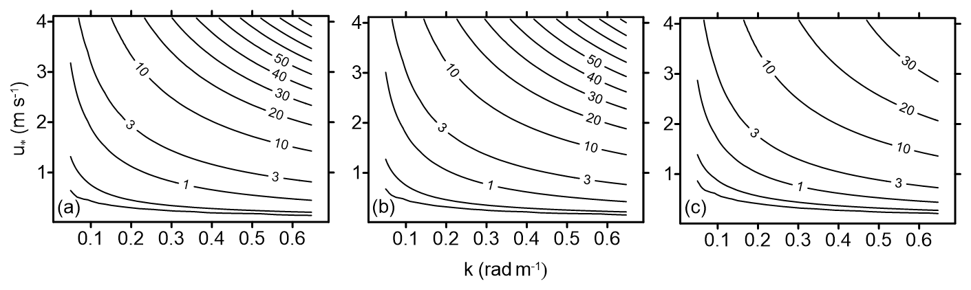
Figure 1 Distribution of growth rate γ as a function of wavenumber and friction velocity (Unit: s⁻¹). (a) $\frac{{\mathit{\tau }}_{\mathrm{w}}}{\mathit{\tau }}=\mathrm{0.2}$; (b) $\frac{{\mathit{\tau }}_{\mathrm{w}}}{\mathit{\tau }}=\mathrm{0.5}$; (c) $\frac{{\mathit{\tau }}_{\mathrm{w}}}{\mathit{\tau }}=\mathrm{0.9}$.

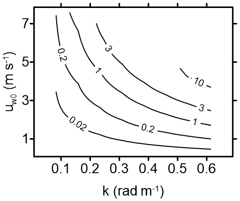
Figure 2 Distribution of dissipation rate γ_tid as a function of wavenumber and wave orbital velocity at sea surface (Unit: s⁻¹).

The unit volume wave energy dissipation rate induced by wave-generated turbulence is $e_{\mathrm{tid}}={〈\frac{k^{\mathrm{2}}}{{\mathit{\pi }}^{\mathrm{2}}\mathit{\epsilon }}{\left(\frac{\partial u_{\mathrm{SM}i}}{\partial x_j}\right)}^{\mathrm{2}}〉}_{\mathrm{SM}}={\mathit{\alpha }}_{\mathrm{wt}}{〈\frac{{\stackrel{\mathrm{‾}}{k}}^{\mathrm{2}}}{{\mathit{\pi }}^{\mathrm{2}}\stackrel{\mathrm{‾}}{\mathit{\epsilon }}}〉}_{\mathrm{SM}}{〈{\left(\frac{\partial u_{\mathrm{SM}i}}{\partial x_j}\right)}^{\mathrm{2}}〉}_{\mathrm{SM}}$ following from Eq. (2), and according the equilibrium solutions of the generation term to the dissipation for wave-generated turbulence (Yuan et al., 2013), the TKE dissipation rate ε_dis can be virtually identical to e_tid, i. e.,

$$\begin{array}{}\text{(18)}& {\mathit{\epsilon }}_{\mathrm{dis}}\approx e_{\mathrm{tid}}={\mathit{\alpha }}_{\mathrm{wt}}{〈{\displaystyle \frac{{\stackrel{\mathrm{‾}}{k}}^{\mathrm{2}}}{{\mathit{\pi }}^{\mathrm{2}}\stackrel{\mathrm{‾}}{\mathit{\epsilon }}}}〉}_{\mathrm{SM}}{〈{\left({\displaystyle \frac{\partial u_{\mathrm{SM}i}}{\partial x_j}}\right)}^{\mathrm{2}}〉}_{\mathrm{SM}}\end{array}$$

There are many studies to verify the modeled TKE dissipation rate ε_dis , generated by shear instability of irregular wind waves or swells, with cruise observations (Yuan et al., 2013; Zhuang et al., 2020, 2021). Here a direct comparison between modeled ε_dis with laboratory observations is performed for monochromatic non-breaking waves. In consideration of an approximate coefficient $\mathrm{7}/\mathrm{8}$ introduced from the minimization relation for the equilibrium solutions (Yuan et al., 2013), the TKE dissipation rate ε_dis can be derived as

$$\begin{array}{}\text{(19)}& \begin{array}{rl}& {\mathit{\epsilon }}_{\mathrm{dis}}\approx {\mathit{\alpha }}_{\mathrm{wt}}{\displaystyle \frac{\mathrm{7}}{\mathrm{8}}}{〈{\displaystyle \frac{{\stackrel{\mathrm{‾}}{k}}^{\mathrm{2}}}{{\mathit{\pi }}^{\mathrm{2}}\stackrel{\mathrm{‾}}{\mathit{\epsilon }}}}〉}_{\mathrm{SM}}{〈{\left({\displaystyle \frac{\partial u_{\mathrm{SM}i}}{\partial x_j}}\right)}^{\mathrm{2}}〉}_{\mathrm{SM}}\\ & ={\displaystyle \frac{\mathrm{7}\sqrt{\mathrm{7}}}{\mathrm{16}}}{\mathit{\alpha }}_{\mathrm{wt}}{A}^{\mathrm{5}}{\mathit{\omega }}^{\mathrm{3}}{K}^{\mathrm{3}}\exp \left\{\mathrm{5}K{x}_{\mathrm{3}}\right\}\end{array}\end{array}$$

where A is the monochromatic wave amplitude at surface.

Two sets of experimental data are selected to verify the modeled TKE dissipation rate ε_dis below. For the first set of laboratory measurements, in order to avoid ambiguity due to wind-caused shear stresses and other dynamic mechanisms, a simple setup for unforced mechanically generated monochromatic wave trains was realized. For the second set of laboratory measurements, wave-induced turbulence with regard to the wind wave, swell and mixed wave conditions, as well as the decreasing tendency of the TKE dissipation rate with layer depth, was conducted for joint comparisons.

The “observed” TKE dissipation rates ε_dis in the first set of experimental data come from the laboratory measurements conducted in the Air-Sea Interaction Saltwater Tank (ASIST) of the University of Miami (Babanin and Haus, 2009; Babanin, 2011), with generated wave trains of f= 1.5 Hz and K_1.5 Hz= 9.82 rad m⁻¹. The significant TKE dissipation rates ε_dis were retrieved from the wavenumber spectra provided by Particle Image Velocimetry (PIV) measurements at the 30 mm layer from the still surface. Their detailed experimental measurements indicate that the turbulence observed must have been directly generated by the waves themselves (Babanin and Haus, 2009). Figure 3 shows the dependence of TKE dissipation rate ε_dis versus wave amplitude A in logarithmic and linear scales respectively, and the solid line is plotted by using Eq. (19) with α_wt=1.0 (Layer depth x₃ varies corresponding to different A). Babanin (2011) interpreted that the “observed” ε_dis are instantaneous values incurred intermittently at the rear-face phase of the wave below the level of the wave trough, and if averaged over the wave period, the estimates of ε_dis have to be divided at least by a factor of 10 and perhaps more. This implies that such intermittent turbulence is still at the stage of quasi-equilibrium level, and the coefficient α_wt=1.0 should be tuned to less than one order of magnitude or more for practical application (Wang et al., 2024).

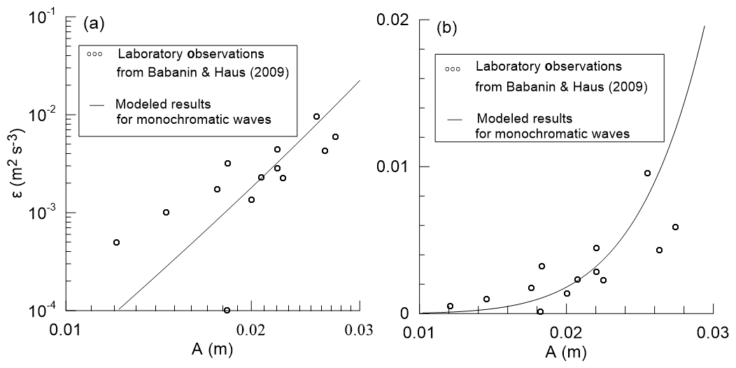
Figure 3 Dependence of TKE dissipation rate ε_dis (denoted as ε in the figure) versus wave amplitude A. Observation data (circles) are digitalized from Babanin and Haus (2009). Dependence (19) is shown with a solid line. Data are plotted in (a) logarithmic scales and (b) linear scales.

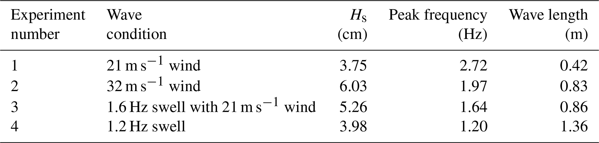
In the second set of experimental data, the “observed” TKE dissipation rates ε_dis with different layer depth come from the laboratory measurements performed inside a wave tank at the Institute of Applied Physics of the Russian Academy of Science, Nizhny Novgorod, Russia (Wei et al., 2018). The tank was equipped with a mechanical wavemaker and a fan, which are used to generate mechanical and wind waves respectively. The vertical surface displacement of the generated wind waves and swell trains were measured by 3 resistancetype wave gages, and series of larger waves are selected for our further comparisons (Table 1).

Table 1 Significant wave height (H_s) and peak frequency for selected wave conditions from Wei et al. (2018).

The TKE dissipation rates ε_dis at different layers from surface were retrieved from the wavenumber spectra provided by underwater 3-D instantaneous velocity measured by using an Acoustic Doppler Velocimeter (SonTek microADV). As Thais and Magnaudet (1996) interpreted their experimental observations, the wave orbital motions, which possess strong vertical gradients, ought to be the dominate role of enhancing of the turbulence production. Figure 4 shows the dependence of TKE dissipation rate ε_dis versus layer depth in linear/logarithmic scale for various wave conditions respectively, and the solid lines are plotted also by using Eq. (19) with α_wt=1.0 (A is the mean amplitude of the highest one-third or one-half waves). The decreasing tendency of modeled ε_dis with layer depth under different wave conditions agrees with that of observations in the upper 0.2 m layers. It should be noted that when the layer depth is larger than 0.25 m, the “observed” ε_dis may be regarded as adaptive noises induced by other dynamic mechanisms.

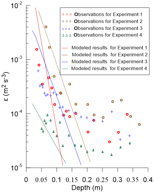
Figure 4 Dependence of TKE dissipation rate ε_dis (denoted as ε in the figure) versus layer depth. Observation data (circles, pluses and triangles) are digitalized from Wei et al. (2018). Dependence (19) is shown with solid lines. Data are plotted in linear/logarithmic scale on the horizontal/vertical axis.

The turbulence production is attributed to the wave-generation conditions. The turbulence observed in the first set of measurement data is directly generated by the waves themselves. While in the second set of measurement data, turbulence generation may be governed by complex dynamical mechanisms, including wave breaking, wind-driven turbulence, Langmuir turbulence, etc., and only the shear instability of wave orbital motions to turbulence is considered here. Preliminary studies indicate that the latter may be the dominant contributor to turbulence, their detailed comparisons are provided in Sect. S1 in the Supplement. The “observed” TKE dissipation rates ε_dis in both sets of measurement data correspond to the instantaneous state when turbulence occurs, and in the above comparative experiments we set the quasi-equilibrium coefficient α_wt=1.0 in our model for the estimates of ε_dis. This introduces uncertainty with regard to phase averaging in practical numerical modeling, which is discussed further in Sect. 4.

2.2 The precise estimation of wave energy loss induced by random wave-breaking

Wave-breaking is another critical dissipation process of ocean waves, which is highly intermittent but simultaneous with wave-generated turbulence stated above. However, the former mechanism still remains not well-understood (Donelan and Yuan, 1994; Young and Babanin, 2006; Yuan et al., 2009). Here in this study, based on the breaking wave statistical method that Cartwright and Longuet-Higgins (1956), Longuet-Higgins (1957), Yuan et al. (1986, 2009) employed under a narrow spectrum assumption for theoretical arguments, we present a more precise approach for estimation of the dissipation-due-to-breaking. Parameterization treatments of the dissipation source function under the assumption of balance between growth and dissipation are discarded, instead of which we derive an improved analytical postbreaking spectrum expression satisfying the kinematic and dynamic wave-breaking onset criterions.

The postbreaking wave spectrum, via the covariance of surface elevation which was assumed to be Gaussian and stationary, was expressed as (Yuan et al., 1986, 1993; Donelan and Yuan, 1994)

$$\begin{array}{}\text{(20)}& E_{\mathrm{b}}(k_{\mathrm{1}},k_{\mathrm{2}})={\mathit{\alpha }}_{\mathrm{b}}E(k_{\mathrm{1}},k_{\mathrm{2}})\end{array}$$

and

$$\begin{array}{}\text{(21)}& {\mathit{\alpha }}_{\mathrm{b}}={\left[\mathrm{1}-{\left({\displaystyle \frac{\mathit{\omega }}{{\mathit{\omega }}_{\mathrm{b}}}}\right)}^{\mathrm{2}}{\left({\displaystyle \frac{\mathrm{2}}{\mathit{\pi }}}\right)}^{\mathrm{1}/\mathrm{2}}{\displaystyle \frac{\mathrm{1}}{L}}\exp \left(-{\displaystyle \frac{L^{\mathrm{2}}}{\mathrm{2}}}\right)\right]}^{\mathrm{2}}\end{array}$$

where $L^{-\mathrm{1}}=\frac{{\mathit{\mu }}_{\mathrm{4}}^{\mathrm{1}/\mathrm{2}}}{g/\mathrm{2}}$ denotes the normalized rms acceleration, $T_{\mathrm{b}}=\mathrm{2}\mathit{\pi }(\frac{{\mathit{\mu }}_{\mathrm{2}}}{{\mathit{\mu }}_{\mathrm{4}}}{)}^{\mathrm{1}/\mathrm{2}}=\mathrm{2}\mathit{\pi }(\frac{{\mathit{\mu }}_{\mathrm{0}}}{{\mathit{\mu }}_{\mathrm{2}}}{)}^{\mathrm{1}/\mathrm{2}}\mathit{\rho }=\mathit{\rho }{T}_{\mathrm{z}}$ and ${\mathit{\omega }}_{\mathrm{b}}=\frac{\mathrm{2}\mathit{\pi }}{T_{\mathrm{b}}}$ denote the mean period or mean frequency of wave maxima, T_z denotes the zero-crossing wave period; ρ denotes a parameter associated with the spectrum width parameter ε_sp, i.e.,

$$\begin{array}{}\text{(22)}& {\displaystyle }{\mathit{\rho }}^{\mathrm{2}}={\displaystyle \frac{{\mathit{\mu }}_{\mathrm{2}}^{\mathrm{2}}}{{\mathit{\mu }}_{\mathrm{0}}{\mathit{\mu }}_{\mathrm{4}}}}\text{(23)}& {\displaystyle }{\mathit{\epsilon }}_{\mathrm{sp}}^{\mathrm{2}}=\mathrm{1}-{\mathit{\rho }}^{\mathrm{2}}\end{array}$$

and μ_i, the ith order moment of the wave spectrum. It should be noted that all the variables stated above are related to the incipient waves, not the postbreaking ones.

So the attenuation coefficient α_b is derived as (The derivation processes to the following Eqs. (24)–(27) are provided in Appendix C)

$$\begin{array}{}\text{(24)}& {\mathit{\alpha }}_{\mathrm{b}}={\left[\mathrm{1}-\mathrm{4}\left(\mathrm{2}\mathit{\pi }{)}^{-\mathrm{1}/\mathrm{2}}{\displaystyle \frac{\mathit{\rho }{\mathit{\omega }}^{\mathrm{2}}{\mathit{\mu }}_{\mathrm{0}}^{\mathrm{1}/\mathrm{2}}}{g}}\exp \right(-{\displaystyle \frac{{\mathit{\rho }}^{\mathrm{2}}}{\mathrm{8}}}{\displaystyle \frac{g^{\mathrm{2}}}{{\mathit{\mu }}_{\mathrm{0}}{\mathit{\omega }}_{\mathrm{z}}^{\mathrm{4}}}})\right]}^{\mathrm{2}}\end{array}$$

where ${\mathit{\omega }}_{\mathrm{z}}=(\frac{{\mathit{\mu }}_{\mathrm{2}}}{{\mathit{\mu }}_{\mathrm{0}}}{)}^{\mathrm{1}/\mathrm{2}}$ denotes the mean zero-crossing wave frequency. The ratio of total energy loss due to wave-breaking is given by

$$\begin{array}{}\text{(25)}& \begin{array}{rl}{r}_{\mathrm{b}}& ={\displaystyle \frac{\int \underset{\mathit{k}}{\int }E(k_{\mathrm{1}},k_{\mathrm{2}})\mathrm{d}{k}_{\mathrm{1}}\mathrm{d}{k}_{\mathrm{2}}-\int \underset{\mathit{k}}{\int }{E}_{\mathrm{b}}(k_{\mathrm{1}},k_{\mathrm{2}})\mathrm{d}{k}_{\mathrm{1}}\mathrm{d}{k}_{\mathrm{2}}}{\int \underset{\mathit{k}}{\int }E(k_{\mathrm{1}},k_{\mathrm{2}})\mathrm{d}{k}_{\mathrm{1}}\mathrm{d}{k}_{\mathrm{2}}}}\\ & \approx \mathrm{8}\left(\mathrm{2}\mathit{\pi }{)}^{-\mathrm{1}/\mathrm{2}}{\displaystyle \frac{\mathit{\rho }{\stackrel{\mathrm{‾}}{\mathit{\omega }}}^{\mathrm{2}}{\mathit{\mu }}_{\mathrm{0}}^{\mathrm{1}/\mathrm{2}}}{g}}\exp \right(-{\displaystyle \frac{{\mathit{\rho }}^{\mathrm{2}}}{\mathrm{8}}}{\displaystyle \frac{g^{\mathrm{2}}}{{\mathit{\mu }}_{\mathrm{0}}{\mathit{\omega }}_{\mathrm{z}}^{\mathrm{4}}}})\end{array}\end{array}$$

where $\stackrel{\mathrm{‾}}{\mathit{\omega }}$ denotes the mean wave frequency with $\stackrel{\mathrm{‾}}{\mathit{\omega }}=(\frac{{\mathit{\mu }}_{\mathrm{2}}}{{\mathit{\mu }}_{\mathrm{0}}}{)}^{\mathrm{1}/\mathrm{2}}={\mathit{\omega }}_{\mathrm{z}}$ here. Babanin (2006) analyzed the measurement records by Yefimov and Khristoforov (1971) and concluded that the breaking ratio of dominant waves was 0.01 %–0.4 %.

In the neighborhood of wave crests ${\mathit{\mu }}_{\mathrm{0}}{\stackrel{\mathrm{‾}}{\mathit{\omega }}}^{\mathrm{2}}\sim \frac{\mathrm{1}}{\mathrm{2}}{c}_{\mathrm{0}}^{\mathrm{2}}$, where c₀ is the characteristic wave speed with $c_{\mathrm{0}}^{\mathrm{2}}=g^{\mathrm{2}}\frac{{\mathit{\mu }}_{\mathrm{0}}^{\mathrm{1}/\mathrm{2}}}{{\mathit{\mu }}_{\mathrm{4}}^{\mathrm{1}/\mathrm{2}}}\mathit{\rho }$ (Yuan et al., 2009), so $\frac{{\stackrel{\mathrm{‾}}{\mathit{\omega }}}^{\mathrm{2}}{\mathit{\mu }}_{\mathrm{0}}^{\mathrm{1}/\mathrm{2}}}{g}=\frac{{\stackrel{\mathrm{‾}}{\mathit{\omega }}}^{\mathrm{2}}{\mathit{\mu }}_{\mathrm{0}}}{g{\mathit{\mu }}_{\mathrm{0}}^{\mathrm{1}/\mathrm{2}}}\sim \frac{c_{\mathrm{0}}^{\mathrm{2}}}{\mathrm{2}g{\mathit{\mu }}_{\mathrm{0}}^{\mathrm{1}/\mathrm{2}}}=\frac{g{\mathit{\mu }}_{\mathrm{2}}}{\mathrm{2}{\mathit{\mu }}_{\mathrm{0}}^{\mathrm{1}/\mathrm{2}}{\mathit{\mu }}_{\mathrm{4}}}=\mathit{\rho }\frac{g}{\mathrm{2}{\mathit{\mu }}_{\mathrm{4}}^{\mathrm{1}/\mathrm{2}}}=\mathit{\rho }L$. This yields r_b∼ρ²L, which agrees with the relative mechanical energy loss per unit sea surface area. Yuan et al. (2009) derived some basic statistics of wave breaking for a narrow spectrum, especially the breaking kinetic and potential energy loss which add up to deduce the breaking mechanical energy loss formulated by introducing the ratio of the former to the latter. Wang et al. (2017, 2018) concluded that the ratio is mainly within the range 3–30, which indicates that there is a disproportion feature between the wave kinetic energy loss and potential one due to wave-breaking. Shi et al. (2025) validated the statistical wave-breaking model across multiple sites from the High Wind Speed Gas Exchange Study (HiWinGS), and concluded that the model is highly effective in capturing the dynamics of whitecap coverage across a range of high sea states. Based on the latest findings, an improved attenuation coefficient by introducing the breaking kinetic energy loss is proposed as follows:

$$\begin{array}{}\text{(26)}& \begin{array}{rl}{\mathit{\alpha }}_{\mathrm{b}}^{\prime }& =\mathrm{1}-\mathit{\rho }{\displaystyle \frac{{\mathit{\omega }}^{\mathrm{2}}{\mathit{\mu }}_{\mathrm{0}}^{\mathrm{1}/\mathrm{2}}}{g}}{\displaystyle \frac{\mathrm{1}}{L}}\left[L\underset{-\mathrm{\infty }}{\overset{-L}{\int }}\exp \left\{-{\displaystyle \frac{\mathrm{1}}{\mathrm{2}}}{Z}^{\mathrm{2}}\right\}\mathrm{d}Z\right.\\ & \left.+\exp \left\{-{\displaystyle \frac{{\mathit{\rho }}^{\mathrm{2}}}{\mathrm{8}}}{\displaystyle \frac{g^{\mathrm{2}}}{{\mathit{\mu }}_{\mathrm{0}}{\mathit{\omega }}_{\mathrm{z}}^{\mathrm{4}}}}\right\}\right]\end{array}\end{array}$$

where the first and second terms in the bracket on the right-hand side are related to the dimensionless breaking kinetic and potential energy loss respectively, $L=\frac{g}{\mathrm{2}{\mathit{\mu }}_{\mathrm{4}}^{\mathrm{1}/\mathrm{2}}}=\frac{\mathit{\rho }}{\mathit{\pi }\mathit{\lambda }}{\left(\frac{H_{\mathrm{S}}}{\stackrel{\mathrm{‾}}{L}}\right)}^{-\mathrm{1}}=\frac{\mathit{\rho }}{\mathrm{2}}\frac{g}{{\mathit{\mu }}_{\mathrm{0}}^{\mathrm{1}/\mathrm{2}}{\mathit{\omega }}_{\mathrm{z}}^{\mathrm{2}}}$, mean wavelength $\stackrel{\mathrm{‾}}{L}=\mathit{\lambda }\frac{g}{\mathrm{2}\mathit{\pi }}{T}_{\mathrm{z}}^{\mathrm{2}}$, $\mathit{\lambda }=\frac{\mathrm{2}}{\mathrm{3}}$ or 0.86 (Kinsman, 2012; Yuan et al., 2009; Xu and Yu, 2001). There is a prominent consistency between Eqs. (26) and (24) under some certain circumstances. Let $\mathit{\theta }\equiv L\underset{-\mathrm{\infty }}{\overset{-L}{\int }}\exp \left\{-\frac{\mathrm{1}}{\mathrm{2}}{Z}^{\mathrm{2}}\right\}\mathrm{d}Z/\exp \left\{-\frac{{\mathit{\rho }}^{\mathrm{2}}}{\mathrm{8}}\frac{g^{\mathrm{2}}}{{\mathit{\mu }}_{\mathrm{0}}{\mathit{\omega }}_{\mathrm{z}}^{\mathrm{4}}}\right\}$ represents the ratio of the kinetic energy loss to the potential one due to wave-breaking (Yuan et al., 2009; Wang et al., 2017, 2018), Eq. (26) can be rewritten as

$$\begin{array}{}\text{(27)}& {\mathit{\alpha }}_{\mathrm{b}}^{\prime }=\mathrm{1}-\mathit{\rho }{\displaystyle \frac{{\mathit{\omega }}^{\mathrm{2}}{\mathit{\mu }}_{\mathrm{0}}^{\mathrm{1}/\mathrm{2}}}{g}}{\displaystyle \frac{\mathrm{1}+\mathit{\theta }}{L}}\exp \left\{-{\displaystyle \frac{{\mathit{\rho }}^{\mathrm{2}}}{\mathrm{8}}}{\displaystyle \frac{g^{\mathrm{2}}}{{\mathit{\mu }}_{\mathrm{0}}{\mathit{\omega }}_{\mathrm{z}}^{\mathrm{4}}}}\right\}\end{array}$$

Suppose that $\frac{H_{\mathrm{S}}}{\stackrel{\mathrm{‾}}{L}}=\frac{\mathrm{1}}{\mathrm{7}},\mathit{\rho }=\mathrm{0.6},\mathit{\theta }=\mathrm{4}$, then $\frac{\mathrm{1}+\mathit{\theta }}{L}=\mathrm{3.216}\sim \mathrm{8}(\mathrm{2}\mathit{\pi }{)}^{-\mathrm{1}/\mathrm{2}}=\mathrm{3.192}$, while the latter coefficient comes originally from the complicated 0–1st order asymptotic expansions of the covariance of surface elevation, i.e. the foundation of the wave-breaking dissipation source function of the original MASNUM wave model. Equations (26) and (27) demonstrate definitely the dominant role of the kinetic energy loss induced by wave-breaking, and the former is applied in the following numerical experiments.

Young and Babanin (2006) obtained the breaking spectrum and nonbreaking spectrum from segments of the comprehensive measurement records in the Australian Shallow Water Experiment (AUSWEX), carried out at Lake George in New South Wales in 1997–2000, and analyzed the spectral difference with the ratio of the two spectra plotted as a function of frequency f in Fig. 5. According to Eq. (26), we also calculate the attenuation coefficient with H_s = 0.45 m, f_p= 0.39 Hz but ρ differs from 0.4 to 0.6. Although there is oscillation mainly caused by survey array of high-precision capacitance wave probes, a decreasing tendency of the “observed” ratio is remarkable from low frequencies to the high frequency f= 5f_p, which imparts the fact that the longer wave scales are more affected by the dominant breaking. The calculated attenuation coefficients correspond to this tendency, which yields valuable insights of the physics of dominant breaking, but the statistical approach is less well-suited for simulating the rapid transient regime of wave breaking as well as for the higher frequency in the equilibrium range. For the higher frequency f>5f_p, there is not the decreasing feature for the “observed” ratio, this can be explained by the statistical equilibrium in the equilibrium range proposed by Phillips (1985) or the short scales' prompt recovery interpreted by Young and Babanin (2006). When Eq. (26) is applied in the 3rd generation wave models, e.g. the MASNUM wave model (Yuan et al., 1991; Yang et al., 2005), though the attenuation coefficient ${\mathit{\alpha }}_{\mathrm{b}}^{\prime }$ approaches to zero for those higher frequencies, the equilibrium wave spectra in the equilibrium range are used to complement the underestimation induced by wave-breaking.

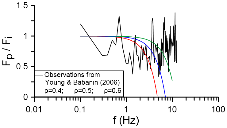
Figure 5 Ratio of the spectra between incipient-breaking and postbreaking waves. Black line: Observations are digitalized from Young and Babanin (2006); Color lines: Calculated ${\mathit{\alpha }}_{\mathrm{b}}^{\prime }$ according to Eq. (26) with ρ=0.4, 0.5, 0.6 respectively.

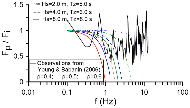
Figure 6 Same as Fig. 5 but for ordinary and high sea states. Observations digitalized from Young and Babanin (2006) are also displayed for comparison. Circles, dashed and solid lines represent different wave states, while colors represent different ρ selected in Eq. (26).

We further evaluate the attenuation coefficients by using Eq. (26) on ordinary and high sea states, which are plotted in Fig. 6. Apart from the significant wave height, the zero-crossing wave period also plays an important role for the quantity of the attenuation coefficient. In addition, it decreases apparently at high sea states, which indicates the wave-breaking intensity is more remarkable.

3 Application implementations on simple duration-limited growth and decay experiments

There remain two undetermined parameters α_wt,ρ in the preceding section, which will be discussed further in Sect. 4. Both of them are chosen as tunable parameters in the duration-limited growth and decay experiments undertook below. The numerical experiments were carried out with the MASNUM wave model (Yuan et al., 1991; Yang et al., 2005), and implemented according to the studies of Janssen et al. (1994). We ran the model for seven days, the first two days with a wind speed of 18.45 m s⁻¹, after which the wind dropped to a value of 5 m s⁻¹. The model integration time step was 30 s, so the growth limiter can be switched off and its impacts need not be considered here.

For simplicity, the parameterization of linear growth in spectral density proposed by Komen et al. (1984) and the quasi-linear one by Janssen (1991) for wind input source function S_in are used respectively. As stated above, coefficient α_wt should be tuned to 0.02–0.2. Wang et al. (2017, 2018) validated the sea surface whitecap courage obtained from the statistical wave-breaking model with the satellite-derived data and proposed that the range of ρ is 0.53–0.59, and this referenced span is used in the following experiments.

To evaluate the scaling behavior of the new dissipation formulations due to wave-generated turbulence and wave-breaking proposed in Sect. 2, as well as their different effects, several numerical experiments are carried out (Table 2). In the original 3rd generation MASNUM wave model described here (Experiment 1), a parameterization proposed by Yuan et al. (1986),Yuan et al. (1993), Donelan and Yuan (1994) is adopted for wave-breaking dissipation source function S_ds, i.e.,

$$\begin{array}{}\text{(28)}& \begin{array}{rl}{S}_{\mathrm{ds}}& =-d_{\mathrm{1}}\widehat{\mathit{\omega }}{\left({\displaystyle \frac{\mathit{\omega }}{\widehat{\mathit{\omega }}}}\right)}^{\mathrm{2}}{\left({\displaystyle \frac{\widehat{\mathit{\alpha }}}{{\widehat{\mathit{\alpha }}}_{\mathrm{PM}}}}\right)}^{\mathrm{1}/\mathrm{2}}\\ & \exp \left\{-d_{\mathrm{2}}(\mathrm{1}-{\mathit{\epsilon }}_{\mathrm{sp}}^{\mathrm{2}}){\displaystyle \frac{{\widehat{\mathit{\alpha }}}_{\mathrm{PM}}}{\widehat{\mathit{\alpha }}}}\right\}E(k_{\mathrm{1}},k_{\mathrm{2}})\end{array}\end{array}$$

where $\widehat{\mathit{\omega }}={\left({\mathit{\mu }}_{-\mathrm{1}}/{\mathit{\mu }}_{\mathrm{0}}\right)}^{-\mathrm{1}},\widehat{\mathit{\alpha }}={\mathit{\mu }}_{\mathrm{0}}{\widehat{\mathit{\omega }}}^{\mathrm{4}}{g}^{-\mathrm{2}}$, ${\widehat{\mathit{\alpha }}}_{\mathrm{PM}}$ is the value of $\widehat{\mathit{\alpha }}$ for a PM spectrum (${\widehat{\mathit{\alpha }}}_{\mathrm{PM}}=\mathrm{3.02}\times {\mathrm{10}}^{-\mathrm{3}})$. Two critical coefficients d₁ and d₂ ($d_{\mathrm{1}}=\mathrm{1.32}\times {\mathrm{10}}^{-\mathrm{4}},d_{\mathrm{2}}=\mathrm{2.61})$ were retrieved through fitting algorithm with the dimensional expression proposed by Komen et al. (1984). The corresponding dissipation term in the WAM-Cycle models is given as.

$$\begin{array}{}\text{(29)}& S_{\mathrm{ds}}=-C_{\mathrm{ds}}\widehat{\mathit{\omega }}{\left({\displaystyle \frac{\mathit{\omega }}{\widehat{\mathit{\omega }}}}\right)}^{\mathrm{2}}{\left({\displaystyle \frac{\widehat{\mathit{\alpha }}}{{\widehat{\mathit{\alpha }}}_{\mathrm{PM}}}}\right)}^{\mathrm{2}}E(k_{\mathrm{1}},k_{\mathrm{2}})\end{array}$$

where C_ds is a constant ($C_{\mathrm{ds}}=\mathrm{2.36}\times {\mathrm{10}}^{-\mathrm{5}})$.

Table 2 Numerical experiments.

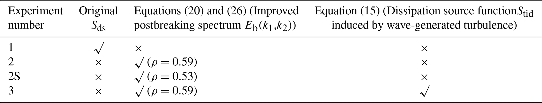
In Experiment 2, instead of this source function S_ds, Eqs. (20) and (26) are used to calculate the postbreaking spectrum, while other unchanged source functions S_in,S_nl, S_bo and S_cu are integrated to obtain the incipient-breaking spectrum. Then the dissipation source function induced by wave-generated turbulence S_tid is further considered in Experiment 3. In the above Experiments 2 and 3, ρ=0.59 is chosen, while ρ=0.53 in the supplemental Experiment 2S for further comparison.

Figures 7 and 8 show the time evolutions of wave height and peak frequency, where the wind input source function in MASNUM wave model was adopted from Komen et al. (1984). The wave height grows during the first two days, then decreases significantly after the wind drops two days later. Results of Janssen et al. (1994) with circle symbols are listed for comparison with Experiment 1–3. Results of the original MASNUM wave model (Experiment 1) are consistent with that of Janssen et al. (1994), but the deviation of wave height may be noted 96h later due to different power of normalized wave slope in the wave-breaking dissipation source function (Yuan et al., 1991; Donelan and Yuan, 1994). The difference of wave height between Experiment 2 and others, both the maximum quantity and swell decay, can be distinguished apparently. Especially the wave height in Experiment 2 hardly changes during the swell decay process, because the mean swell steepness becomes small gradually and ${\mathit{\alpha }}_{\mathrm{b}}^{\prime }\sim \mathrm{1.0}$ in Eqs. (20) and (26). This indicates that the wave energy loss induced by wave-breaking is inadequate, and the role of prior proposed parameterizations for wave-breaking dissipation may be overestimated in the previous studies. Besides the effect of postbreaking wave spectrum, the dissipation source function induced by wave-generated turbulence S_tid is incorporated in Experiment 3. The corresponding modeled wave height and peak frequency are also listed in Figs. 7 and 8, in which different α_wt= 0.05 or 0.06 is selected to highlight its effect. Discrepancies for the maximum of wave height and swell decay are reduced much than that of Experiment 2, and its variation has an analogous trend with that of Janssen et al. (1994).

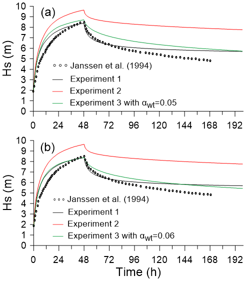
Figure 7 Time evolution of wave height over a seven day period. Modeled data (circles) are digitalized from Janssen et al. (1994). After two days the wind drops. Notice the decay in wave height during the last five days when the waves are considered as swell. (a) α_wt=0.05; (b) α_wt=0.06.

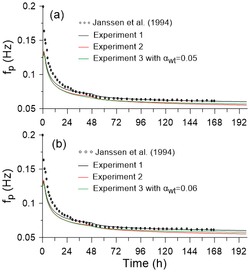
Figure 8 Time evolution of peak frequency over a seven day period. Modeled data (circles) are digitalized from Janssen et al. (1994). After two days the wind drops. Notice the decay in the slight shift in peak frequency during the last five days when the waves are considered as swell. (a) α_wt=0.05; (b) α_wt=0.06.

Figure 9 shows the time evolution of wave height, where the wind input source function in MASNUM wave model was adopted from Janssen (1991). Similar interpretation stated above can be obtained, besides that the effect of postbreaking wave spectrum is still inadequate even for that in the supplemental Experiment 2S where ρ=0.53.

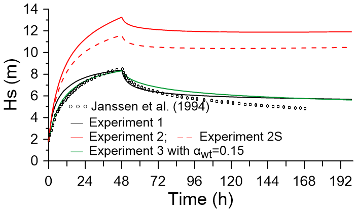
Figure 9 Same as Fig. 7 but the wind input source function in MASNUM wave model was adopted from Janssen (1991) and α_wt=0.15.

4 Discussions

The analytical approaches and the corresponding comparisons to laboratory or in-lake site measurements improve further understandings of wave energy dissipation due to wave-breaking and wave-generated turbulence. This study still exhibits some deficiencies and needs to be addressed on comparative assessments and metrics to previous formulations, as well as evaluations of scaling behavior of the new model, etc. Model validation is tentative and requires future enhanced observations correspondingly. Moreover, there remain problems to be addressed that ρ,α_wt are chosen as constants in this study. Parameter ρ is associated with the spectrum width ε_sp. And according to the statistical theory of breaking waves (Cartwright and Longuet-Higgins, 1956; Longuet-Higgins, 1957; Yuan et al., 1986, 2009), both parameters ρ,ε_sp should be referred to those of incipient-breaking spectrum, which is obtained as an intermediate variable in our model where all source functions are integrated except for the energy loss induced by wave-breaking. In fact, the observed or model outputted wave spectrum would respond to the postbreaking wave spectrum (Donelan and Yuan, 1994). So the prior-to-breaking parameter ρ or ε_sp is currently still poorly understood. Moreover, Lamarre and Melville (1991), Melville et al. (1992) showed that 30 %–50 % of energy lost by breaking waves is expended on entraining bubbles into the water against buoyancy forces, and the residue contributes to the turbulence generation. The interaction mechanism of the breaking-induced turbulence with the progressive waves is also unknown. It should also be mentioned that the whitecap model originally proposed by Hasselmann (1974) is an after-breaking class model, and its inherent assumptions need experimental verification (Young and Babanin, 2006). The whitecaps are situated on the forward faces of the waves, exert a downward pressure on the upward moving water, but the direct and precise estimates of their negative work on the waves need further studies. Given the intricate interactions state above, in our model proposed here, the choice of ρ as a tuned parameter is tentative for numerical implementation.

The constant α_wt is chosen in such a way as a tuned coefficient that it implies the quasi-equilibrium level of wave-generated turbulence, and physically it depends on the normalized shear instability strength of wave motion and further relates to the normalized higher-order moment of wave spectrum (see also Eqs. 7–8). Therefore it is certainly not constant at any instant t in real-world scenarios and its reasonable parameterization should be further studied in the future. This idea is quite similar to the wave-amplitude-based Reynolds number proposed by Babanin (2006), its critical wave Reynolds number for wave-induced turbulence can reach down to a lower margin, Re_wave ∼ 1000, from a series of laboratory experiments (Babanin and Haus, 2009; Dai, et al., 2010). But the appropriate dissipation rate for model implements cannot be inferred from the wave Reynolds number alone and was approached by experimental means (Babanin, 2011; Zieger et al., 2015; Liu, et al., 2019). The gradient Richardson number R_g may be a more appropriate dependency factor for the coefficient α_wt, which needs further perspectives. If the gradient Richardson number R_g is smaller than a critical value $R_{\mathrm{g}}^{\mathrm{c}}$, instability of the flow occurs, i.e.,

$$R_{\mathrm{g}}={\displaystyle \frac{{\widehat{N}}_{\mathrm{3}}^{\mathrm{2}}}{{\left|\frac{\partial u_{\mathrm{SM}\mathit{\alpha }}}{\partial x_{\mathrm{3}}}\right|}^{\mathrm{2}}}}<R_{\mathrm{g}}^{\mathrm{c}},\mathit{\alpha }=\mathrm{1},\mathrm{2}$$

where ${\widehat{N}}_{\mathrm{3}}^{\mathrm{2}}=-g\frac{\partial }{\partial x_{\mathrm{3}}}\left(\frac{\widehat{\mathit{\rho }}}{{\mathit{\rho }}_{\mathrm{0}}}\right)$, the Brunt–Väisälä frequency. Below we let ${\widehat{N}}_{\mathrm{3}}=$ const ≈0.01 rad s⁻¹ in the upper layers and the critical value $R_{\mathrm{g}}^{\mathrm{c}}\approx \mathrm{1}/\mathrm{2}$ (Baumert and Peters, 2000; Baumert et al., 2005). For a monochromatic non-breaking wave $\mathit{\zeta }=\mathit{\eta }\cos (k_{\mathit{\alpha }}{x}_{\mathit{\alpha }}-\mathit{\omega }t)$, which is deemed as a base motion in the framework of the ocean dynamic system, the instability criterion is simplified as

$${\widehat{N}}_{\mathrm{3}}^{\mathrm{2}}<R_{\mathrm{g}}^{\mathrm{c}}{\mathit{\omega }}^{\mathrm{2}}{\left(AK\right)}^{\mathrm{2}}\exp \left(\mathrm{2}K{x}_{\mathrm{3}}\right){\cos }^{\mathrm{2}}(k_{\mathit{\alpha }}{x}_{\mathit{\alpha }}-\mathit{\omega }t)$$

We roughly estimate the critical instability depth induced by the monochromatic waves (Table 3), Fig. 10 shows the dependence of the gradient Richardson number versus layer depth for Case 1 in Table 3. Below the wave crests and troughs, there exist bowl-shaped instability regions, which agree to the experimentally observed instantaneous turbulence incurred intermittently at the rear face of the progressive wave profile, but the breaking-in-progress turbulence develops at the front face (Babanin and Haus, 2009; Babanin, 2011). The coefficient α_wt is qualitatively related to the two-dimensional instability area proportion as shown in Fig. 10 or the instability volume proportion beneath the wave surface in real scenarios, which requires further research.

Table 3 Critical instability depth induced by the monochromatic waves.

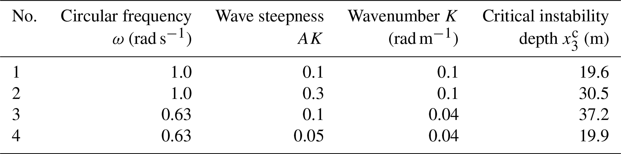
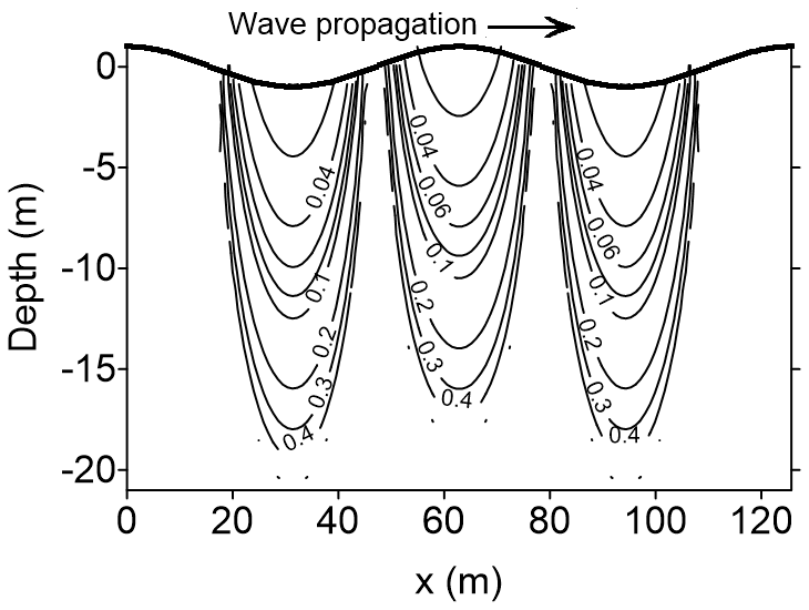
Figure 10 Dependence of the gradient Richardson number versus layer depth for Case 1 in Table 3.

Finally, some limitations of underlying assumptions in our theoretical arguments require further discussions. In the k − ε type eddy viscosity model of wave-generated turbulence, the turbulence timescale is assumed to be shorter than wave period. Therefore, the interaction of turbulence at other scales with ocean waves, which also accounts for a significant fraction of the energy losses of the wave field, is not included in our practical numerical wave model. The quasi-equilibrium assumption of wave-generated turbulence poses the problem of an undetermined coefficient, which needs further elaborations especially essential precise measurements. The linear non-breaking wave theory applied to construct analytical solutions for the turbulence generation is an acceptable assumption in the general case of weakly nonlinear situations, and the scale estimation via the shear instability of wave orbital motions only represents a major portion of the turbulent production in the upper ocean. As stated by Yuan et al. (2009), since the wave spectrum in real-world scenarios is not actually narrow, the breaking wave statistical method under a narrow spectrum assumption is not precise enough to estimate the attenuation coefficient for the postbreaking wave spectrum.

5 Conclusions

The ocean wave energy dissipation is the least understood of the major source terms, previous approaches to estimate the dissipation source function depended on an incomplete description of the physics of the processes including wave-breaking and wave-turbulence interaction. The latest observational efforts offer a possible approach to explore the underlying comprehensive mechanisms.

In the present paper, we attempted to explore the dissipation effects of wave-generated turbulence reacting on ocean waves, and to estimate the energy loss due to wave-breaking via an improved postbreaking spectrum expression based on the breaking wave statistical method. Two new source functions for the above two dissipation processes are proposed and compared respectively to the laboratory or in-lake observations tentatively in Sect. 2, and their different dissipation effects are experimentally analyzed in Sect. 3.

The main conclusion of the study is that we propose an analytical dissipation source function induced by wave-generated turbulence S_tid formulated by Eq. (15), together with an improved postbreaking spectrum expression E_b(k₁,k₂) by Eqs. (20) and (26). The former dissipation term represents the feedback of imparting of wave shear instability generations on turbulence, and the latter expression depicts the intermittent wave-breaking events. Sum of both contributions play critical role of wave energy dissipation.

Here in this paper we roughly estimate the effects of the above two dissipation mechanisms in simple duration-limited growth and decay experiments. Calibration and verification against a series of academic and realistic simulations, including the fetch/duration-limited cases, turning wind (e.g. cold waves or monsoon)/rotatory wind (e.g. extratropical or tropical cyclone) conditions, numerical hindcast and operational forecast in regional and global oceans, will be pursued in our future project, together with considering other concerned dissipation mechanisms.

Appendix A: Brief derivation of Eq. (1)

In the comprehensive framework of the ocean dynamic system comprised of wave-like motions, eddy-like motions and circulation, which are controlled by dynamic gravity balance, static gravity balance and geotropic balance respectively, ocean turbulence, highly random perturbations due to strong nonlinear advections in the foregoing three sub-systems, interacts with larger scale motions including the advection transport and shear instability generation of large-scale dynamic processes as well as the mixing effect in the form of its transport flux residual on the latter (Yuan et al., 2012; Yuan, 2024). More comprehensive governing equations for wave motion were derived under the assumption that turbulence timescale is much shorter than wave period and formulated in tensor expression as follows (Yuan et al., 2012; Yuan, 2024):

$$\begin{array}{}\text{(A1)}& {\displaystyle \frac{\partial u_{\mathrm{SM}j}}{\partial x_j}}=\mathrm{0},\text{(A2)}& {\displaystyle }\begin{array}{rl}& {\displaystyle \frac{\partial u_{\mathrm{SM}i}}{\partial t}}+{\widehat{U}}_j{\displaystyle \frac{\partial u_{\mathrm{SM}i}}{\partial x_j}}+u_{\mathrm{SM}j}{\displaystyle \frac{\partial {\widehat{U}}_i}{\partial x_j}}+{\displaystyle \frac{\partial }{\partial x_j}}\\ & \left(u_{\mathrm{SM}j}{u}_{\mathrm{SM}i}-{〈u_{\mathrm{SM}j}{u}_{\mathrm{SM}i}〉}_{\mathrm{SM}}\right)-\mathrm{2}{\mathit{\epsilon }}_{ijk}{u}_{\mathrm{SM}j}{\mathrm{\Omega }}_k\\ & =-{\displaystyle \frac{\mathrm{1}}{{\mathit{\rho }}_{\mathrm{0}}}}{\displaystyle \frac{\partial p_{\mathrm{SM}}}{\partial x_i}}-g{\displaystyle \frac{{\mathit{\rho }}_{\mathrm{SM}}}{{\mathit{\rho }}_{\mathrm{0}}}}{\mathit{\delta }}_{\mathrm{3}i}\\ & +{\displaystyle \frac{\partial }{\partial x_j}}\left({\mathit{\nu }}_{\mathrm{0}}{\displaystyle \frac{\partial u_{\mathrm{SM}i}}{\partial x_j}}\right)+{\displaystyle \frac{\partial }{\partial x_j}}\\ & \left[-\left({〈u_{\mathrm{SS}j}{u}_{\mathrm{SS}i}〉}_{\mathrm{SS}}-{〈{〈u_{\mathrm{SS}j}{u}_{\mathrm{SS}i}〉}_{\mathrm{SS}}〉}_{\mathrm{SM}}\right)\right],\end{array}\text{(A3)}& {\displaystyle }\begin{array}{rl}& {\displaystyle \frac{\partial {\mathit{\rho }}_{\mathrm{SM}}}{\partial t}}+{\widehat{U}}_j{\displaystyle \frac{\partial {\mathit{\rho }}_{\mathrm{SM}}}{\partial x_j}}+u_{\mathrm{SM}j}{\displaystyle \frac{\partial \widehat{\mathit{\rho }}}{\partial x_j}}+{\displaystyle \frac{\partial }{\partial x_j}}\\ & \left(u_{\mathrm{SM}j}{\mathit{\rho }}_{\mathrm{SM}}-{〈u_{\mathrm{SM}j}{\mathit{\rho }}_{\mathrm{SM}}〉}_{\mathrm{SM}}\right)={\displaystyle \frac{\partial }{\partial x_j}}\left(K_{\mathrm{0}}{\displaystyle \frac{\partial {\mathit{\rho }}_{\mathrm{SM}}}{\partial x_j}}\right)\\ & +{\displaystyle \frac{\partial }{\partial x_j}}\left[-\left({〈u_{{\mathrm{SS}}_j}{\mathit{\rho }}_{\mathrm{S}S}〉}_{\mathrm{S}S}-{〈{〈u_{{\mathrm{SS}}_j}{\mathit{\rho }}_{\mathrm{SS}}〉}_{\mathrm{SS}}〉}_{\mathrm{SM}}\right)\right]\\ & +Q_{{\mathit{\rho }}_{\mathrm{SM}}},\end{array}\end{array}$$

where $u_{\mathrm{SM}i},i=\mathrm{1},\mathrm{2},\mathrm{3};{\mathit{\rho }}_{\mathrm{SM}}$ denote the ocean wave components, ${\widehat{U}}_i,i=\mathrm{1},\mathrm{2},\mathrm{3};\widehat{T},\widehat{s},\widehat{p},\widehat{\mathit{\rho }}$ denote the background current components, ρ₀ is the basin mean water density; ${\mathit{\nu }}_{\mathrm{0}},K_{\mathrm{0}},D_{\mathrm{0}}$ denote the molecular viscosity, thermal and diffusion coefficients; $Q_{{\mathit{\rho }}_{\mathrm{SM}}}$ denotes the thermal source due to temperature and salinity perturbations; $\langle \cdot {\rangle }_{\mathrm{SS}},\langle \cdot {\rangle }_{\mathrm{SM}}$ denote the Reynolds averages on the turbulence and wave motions respectively. Hereafter, other symbols have their usual meaning.

Multiplying Eq. (A2) by ρ₀u_SMi and Eq. (A3) by ρ_SM, after some manipulation, yields the unit volume mechanical kinetic energy and potential energy respectively. Sum of both energy terms and Reynolds averaged on the wave motion reduce to

$$\begin{array}{}\text{(A4)}& \begin{array}{l}\frac{\partial }{\partial t}{〈\frac{{\mathit{\rho }}_{\mathrm{0}}{u}_{\mathrm{SM}i}^{\mathrm{2}}}{\mathrm{2}}+\frac{g^{\mathrm{2}}{\mathit{\rho }}_{\mathrm{SM}}^{\mathrm{2}}}{\mathrm{2}{\mathit{\rho }}_{\mathrm{0}}{\widehat{N}}_{\mathrm{3}}^{\mathrm{2}}}〉}_{\mathrm{SM}}+{〈\left({\widehat{U}}_j+u_{\mathrm{SM}j}\right)\frac{\partial }{\partial x_j}\left(\frac{{\mathit{\rho }}_{\mathrm{0}}{u}_{\mathrm{SM}i}^{\mathrm{2}}}{\mathrm{2}}+\frac{g^{\mathrm{2}}{\mathit{\rho }}_{\mathrm{SM}}^{\mathrm{2}}}{\mathrm{2}{\mathit{\rho }}_{\mathrm{0}}{\widehat{N}}_{\mathrm{3}}^{\mathrm{2}}}\right)〉}_{\mathrm{SM}}+\frac{\partial }{\partial x_i}{〈p_{\mathrm{SM}}{u}_{\mathrm{SM}i}〉}_{\mathrm{SM}}\\ =-{\mathit{\rho }}_{\mathrm{0}}{〈u_{\mathrm{SM}i}{u}_{\mathrm{SM}j}〉}_{\mathrm{SM}}\frac{\partial {\widehat{U}}_i}{\partial x_j}+g{〈{\mathit{\rho }}_{\mathrm{SM}}{u}_{\mathrm{SM}\mathit{\beta }}〉}_{\mathrm{SM}}\frac{{\widehat{N}}_{\mathit{\beta }}^{\mathrm{2}}}{{\widehat{N}}_{\mathrm{3}}^{\mathrm{2}}}+\frac{g^{\mathrm{2}}}{{\mathit{\rho }}_{\mathrm{0}}{\widehat{N}}_{\mathrm{3}}^{\mathrm{2}}}{〈{\mathit{\rho }}_{\mathrm{SM}}{Q}_{{\mathit{\rho }}_{\mathrm{SM}}}〉}_{\mathrm{SM}}\\ +\left[\begin{array}{l}{〈{\mathit{\rho }}_{\mathrm{0}}{u}_{\mathrm{SM}i}\frac{\partial }{\partial x_j}\left({\mathit{\nu }}_{\mathrm{0}}\frac{\partial u_{\mathrm{SM}i}}{\partial x_j}\right)〉}_{\mathrm{SM}}+{〈\frac{g^{\mathrm{2}}{\mathit{\rho }}_{\mathrm{SM}}}{{\mathit{\rho }}_{\mathrm{0}}{\widehat{N}}_{\mathrm{3}}^{\mathrm{2}}}\frac{\partial }{\partial x_j}\left(K_{\mathrm{0}}\frac{\partial {\mathit{\rho }}_{\mathrm{SM}}}{\partial x_j}\right)〉}_{\mathrm{SM}}\\ +{〈{\mathit{\rho }}_{\mathrm{0}}{u}_{\mathrm{SM}i}\frac{\partial }{\partial x_j}\left(-{〈u_{\mathrm{SS}j}{u}_{\mathrm{SS}i}〉}_{\mathrm{SS}}\right)〉}_{\mathrm{SM}}+{〈\frac{g^{\mathrm{2}}{\mathit{\rho }}_{\mathrm{SM}}}{{\mathit{\rho }}_{\mathrm{0}}{\widehat{N}}_{\mathrm{3}}^{\mathrm{2}}}\frac{\partial }{\partial x_j}\left(-{〈u_{{\mathrm{SS}}_j}{\mathit{\rho }}_{\mathrm{SS}}〉}_{\mathrm{SS}}\right)〉}_{\mathrm{SM}}\end{array}\right],\end{array}\end{array}$$

Based on closure assumptions of the k−ε type eddy viscosity model (Baumert et al., 2005; Yuan et al., 2013), Eq. (A4) can be written as

$$\begin{array}{}\text{(A5)}& \begin{array}{l}\frac{\partial }{\partial t}{〈\frac{{\mathit{\rho }}_{\mathrm{0}}{u}_{\mathrm{SM}i}^{\mathrm{2}}}{\mathrm{2}}+\frac{g^{\mathrm{2}}{\mathit{\rho }}_{\mathrm{SM}}^{\mathrm{2}}}{\mathrm{2}{\mathit{\rho }}_{\mathrm{0}}{\widehat{N}}_{\mathrm{3}}^{\mathrm{2}}}〉}_{\mathrm{SM}}+{〈\left({\widehat{U}}_j+u_{\mathrm{SM}j}\right)\frac{\partial }{\partial x_j}\left(\frac{{\mathit{\rho }}_{\mathrm{0}}{u}_{\mathrm{SM}i}^{\mathrm{2}}}{\mathrm{2}}+\frac{g^{\mathrm{2}}{\mathit{\rho }}_{\mathrm{SM}}^{\mathrm{2}}}{\mathrm{2}{\mathit{\rho }}_{\mathrm{0}}{\widehat{N}}_{\mathrm{3}}^{\mathrm{2}}}\right)〉}_{\mathrm{SM}}+\frac{\partial }{\partial x_i}{〈p_{\mathrm{SM}}{u}_{\mathrm{SM}i}〉}_{\mathrm{SM}}\\ =\left(-{\mathit{\rho }}_{\mathrm{0}}{〈u_{\mathrm{SM}i}{u}_{\mathrm{SM}j}〉}_{\mathrm{SM}}\frac{\partial {\widehat{U}}_i}{\partial x_j}+g{〈{\mathit{\rho }}_{\mathrm{SM}}{u}_{\mathrm{SM}\mathit{\alpha }}〉}_{\mathrm{SM}}\frac{{\widehat{N}}_{\mathit{\alpha }}^{\mathrm{2}}}{{\widehat{N}}_{\mathrm{3}}^{\mathrm{2}}}\right)+\frac{g^{\mathrm{2}}}{{\mathit{\rho }}_{\mathrm{0}}{\widehat{N}}_{\mathrm{3}}^{\mathrm{2}}}{〈{\mathit{\rho }}_{\mathrm{SM}}{Q}_{{\mathit{\rho }}_{\mathrm{SM}}}〉}_{\mathrm{SM}}\\ +\left\{\begin{array}{l}\frac{\partial }{\partial x_j}{〈\left({\mathit{\nu }}_{\mathrm{0}}+\frac{k^{\mathrm{2}}}{{\mathit{\pi }}^{\mathrm{2}}\mathit{\epsilon }}\right)\frac{\partial }{\partial x_j}\left(\frac{{\mathit{\rho }}_{\mathrm{0}}{u}_{\mathrm{SM}i}^{\mathrm{2}}}{\mathrm{2}}\right)〉}_{\mathrm{SM}}+\frac{\partial }{\partial x_j}{〈\left(K_{\mathrm{0}}+\frac{\mathrm{1}}{{\mathit{\sigma }}_{\mathrm{0}}}\frac{k^{\mathrm{2}}}{{\mathit{\pi }}^{\mathrm{2}}\mathit{\epsilon }}\right)\frac{\partial }{\partial x_j}\left(\frac{g^{\mathrm{2}}{\mathit{\rho }}_{\mathrm{SM}}^{\mathrm{2}}}{\mathrm{2}{\mathit{\rho }}_{\mathrm{0}}{\widehat{N}}_{\mathrm{3}}^{\mathrm{2}}}\right)〉}_{\mathrm{SM}}\\ -{〈{\mathit{\rho }}_{\mathrm{0}}\left({\mathit{\nu }}_{\mathrm{0}}+\frac{k^{\mathrm{2}}}{{\mathit{\pi }}^{\mathrm{2}}\mathit{\epsilon }}\right){\left(\frac{\partial u_{\mathrm{SM}i}}{\partial x_j}\right)}^{\mathrm{2}}〉}_{\mathrm{SM}}-{〈\frac{g^{\mathrm{2}}}{{\mathit{\rho }}_{\mathrm{0}}{\widehat{N}}_{\mathrm{3}}^{\mathrm{2}}}\left(K_{\mathrm{0}}+\frac{\mathrm{1}}{{\mathit{\sigma }}_{\mathrm{0}}}\frac{k^{\mathrm{2}}}{{\mathit{\pi }}^{\mathrm{2}}\mathit{\epsilon }}\right){\left(\frac{\partial {\mathit{\rho }}_{\mathrm{SM}}}{\partial x_j}\right)}^{\mathrm{2}}〉}_{\mathrm{SM}}\end{array}\right\}\end{array}\end{array}$$

where ${\widehat{N}}_i^{\mathrm{2}}=-g\frac{\partial }{\partial x_i}\left(\frac{\widehat{\mathit{\rho }}}{{\mathit{\rho }}_{\mathrm{0}}}\right),i=\mathrm{1},\mathrm{2},\mathrm{3}$ denote the Brunt–Väisälä frequency components; ${\mathit{\sigma }}_{\mathrm{0}}=\frac{\mathrm{1}}{\mathrm{2}}$ the Prandtl number; k,ε the kinetic energy and the dissipation rate of ocean turbulence, which is generated by shear instability of background current, Stokes drift and wave orbital motions in the upper layers. Here in this study, only the wave-generated turbulence is considered. Its analytical mixing coefficients were proposed through equilibrium solutions of the second-order turbulence closure model between the wave motion shear instability generations and the TKE dissipations (Yuan et al., 2013).

Appendix B: Brief derivations of Eqs. (12), (15) and (19)

Yuan et al. (2013) proposed equilibrium solutions of the k− ε type eddy viscosity model from the minimization relation, and the TKE dissipation rate ε can be expressed as

$$\begin{array}{}\text{(B1)}& \stackrel{\mathrm{‾}}{\mathit{\epsilon }}\approx {\displaystyle \frac{\mathrm{7}}{\mathrm{8}}}{\displaystyle \frac{{\stackrel{\mathrm{‾}}{k}}^{\mathrm{2}}}{{\mathit{\pi }}^{\mathrm{2}}\stackrel{\mathrm{‾}}{\mathit{\epsilon }}}}{\left({\displaystyle \frac{\partial u_{\mathrm{SM}i}}{\partial x_j}}\right)}^{\mathrm{2}}\end{array}$$

The approximate coefficient $\mathrm{7}/\mathrm{8}$ indicates that the shear instability generation of surface waves is the dominant source of the turbulence in the upper ocean. Based the mixing length of ${\stackrel{\mathrm{‾}}{l}}_{\mathrm{D}}=\frac{{\stackrel{\mathrm{‾}}{k}}^{\mathrm{3}/\mathrm{2}}}{{\mathit{\pi }}^{\mathrm{3}/\mathrm{2}}\stackrel{\mathrm{‾}}{\mathit{\epsilon }}}$ (Baumert et al., 2005), $\stackrel{\mathrm{‾}}{k},\stackrel{\mathrm{‾}}{\mathit{\epsilon }}$ are formulated conveniently as

$$\begin{array}{c}{\displaystyle }\stackrel{\mathrm{‾}}{k}={\displaystyle \frac{\mathrm{7}}{\mathrm{8}}}\mathit{\pi }{\stackrel{\mathrm{‾}}{l}}_{\mathrm{D}}^{\mathrm{2}}{\left({\displaystyle \frac{\partial u_{\mathrm{SM}i}}{\partial x_j}}\right)}^{\mathrm{2}}\\ {\displaystyle }\stackrel{\mathrm{‾}}{\mathit{\epsilon }}={\left({\displaystyle \frac{\mathrm{7}}{\mathrm{8}}}\right)}^{\mathrm{3}/\mathrm{2}}{\stackrel{\mathrm{‾}}{l}}_{\mathrm{D}}^{\mathrm{2}}{\left(\left|{\displaystyle \frac{\partial u_{\mathrm{SM}i}}{\partial x_j}}\right|\right)}^{\mathrm{3}}\end{array}$$

Then the mixing coefficient ${〈\frac{{\stackrel{\mathrm{‾}}{k}}^{\mathrm{2}}}{{\mathit{\pi }}^{\mathrm{2}}\stackrel{\mathrm{‾}}{\mathit{\epsilon }}}〉}_{\mathrm{SM}}$ is expressed as

$$\begin{array}{}\text{(B2)}& {〈{\displaystyle \frac{{\stackrel{\mathrm{‾}}{k}}^{\mathrm{2}}}{{\mathit{\pi }}^{\mathrm{2}}\stackrel{\mathrm{‾}}{\mathit{\epsilon }}}}〉}_{\mathrm{SM}}={\left({\displaystyle \frac{\mathrm{7}}{\mathrm{8}}}\right)}^{\mathrm{1}/\mathrm{2}}{〈{\stackrel{\mathrm{‾}}{l}}_{\mathrm{D}}^{\mathrm{2}}〉}_{\mathrm{SM}}{〈\left|{\displaystyle \frac{\partial u_{\mathrm{SM}i}}{\partial x_j}}\right|〉}_{\mathrm{SM}}\end{array}$$

Yuan et al. (2013) discussed the relation of the classical Prandtl mixing-length theory (Yuan et al., 1999) with the equilibrium solution of the k−ε type eddy viscosity model by the available 12 groups of field data measurements. Here in this study, only the wave-generated turbulence is considered, so we let

$$\begin{array}{}\text{(B3)}& {\stackrel{\mathrm{‾}}{l}}_{\mathrm{D}}\approx \left|\int \underset{\mathit{k}}{\int }A{\displaystyle \frac{\cosh K(\widehat{H}+x_{\mathrm{3}})}{\sinh K\widehat{H}}}\exp \left\{i\left(\mathit{k}\cdot \mathit{r}-\mathit{\omega }t\right)\right\}\mathrm{d}\mathit{k}\right|\end{array}$$

where the wavenumber vector $\mathit{k}=\left(k_{\mathrm{1}},k_{\mathrm{2}}\right)$ with $K=\sqrt{k_{\mathrm{1}}^{\mathrm{2}}+k_{\mathrm{2}}^{\mathrm{2}}}$, $\mathit{r}=\left(x_{\mathrm{1}},x_{\mathrm{2}}\right)$. ω denotes the radian frequency, and A, the wave amplitude. ${〈{\stackrel{\mathrm{‾}}{l}}_{\mathrm{D}}^{\mathrm{2}}〉}_{\mathrm{SM}},{〈\frac{\partial u_{\mathrm{SM}i}}{\partial x_j}\frac{\partial u_{\mathrm{SM}i}}{\partial x_j}〉}_{\mathrm{SM}}$ can be expressed in wavenumber spectrum as

$$\begin{array}{c}{\displaystyle }{〈{\stackrel{\mathrm{‾}}{l}}_{\mathrm{D}}^{\mathrm{2}}〉}_{\mathrm{SM}}\approx \int \underset{\mathit{k}}{\int }E(k_{\mathrm{1}},k_{\mathrm{2}}){\displaystyle \frac{{\cosh }^{\mathrm{2}}K(\widehat{H}+x_{\mathrm{3}})}{{\sinh }^{\mathrm{2}}K\widehat{H}}}\mathrm{d}{k}_{\mathrm{1}}\mathrm{d}{k}_{\mathrm{2}}\\ {\displaystyle }\begin{array}{rl}& {〈{\displaystyle \frac{\partial u_{\mathrm{SM}i}}{\partial x_j}}{\displaystyle \frac{\partial u_{\mathrm{SM}i}}{\partial x_j}}〉}_{\mathrm{SM}}=\int \underset{\mathit{k}}{\int }\mathrm{2}{\mathit{\omega }}^{\mathrm{2}}{K}^{\mathrm{2}}{\displaystyle \frac{\cosh \mathrm{2}K(\widehat{H}+x_{\mathrm{3}})}{{\sinh }^{\mathrm{2}}K\widehat{H}}}\\ & E(k_{\mathrm{1}},k_{\mathrm{2}})\mathrm{d}{k}_{\mathrm{1}}\mathrm{d}{k}_{\mathrm{2}}\end{array}\end{array}$$

Then the mixing coefficient is reduced to

$$\begin{array}{}\text{(B4)}& \begin{array}{rl}& {〈{\displaystyle \frac{{\stackrel{\mathrm{‾}}{k}}^{\mathrm{2}}}{{\mathit{\pi }}^{\mathrm{2}}\stackrel{\mathrm{‾}}{\mathit{\epsilon }}}}〉}_{\mathrm{SM}}={\displaystyle \frac{\sqrt{\mathrm{7}}}{\mathrm{2}}}\int \underset{\mathit{k}}{\int }E(k_{\mathrm{1}},k_{\mathrm{2}}){\displaystyle \frac{{\cosh }^{\mathrm{2}}K(\widehat{H}+x_{\mathrm{3}})}{{\sinh }^{\mathrm{2}}K\widehat{H}}}\mathrm{d}{k}_{\mathrm{1}}\mathrm{d}{k}_{\mathrm{2}}\\ & {\left(\int \underset{\mathit{k}}{\int }{\mathit{\omega }}^{\mathrm{2}}{K}^{\mathrm{2}}{\displaystyle \frac{\cosh \mathrm{2}K(\widehat{H}+x_{\mathrm{3}})}{{\sinh }^{\mathrm{2}}K\widehat{H}}}E(k_{\mathrm{1}},k_{\mathrm{2}})\mathrm{d}{k}_{\mathrm{1}}\mathrm{d}{k}_{\mathrm{2}}\right)}^{\mathrm{1}/\mathrm{2}}\end{array}\end{array}$$

which is Eq. (12) in Sect. 2.1.

For deep water depth, $\frac{\cosh K(\widehat{H}+x_{\mathrm{3}})}{\sinh K\widehat{H}}\sim \exp \mathit{\left\{}K{x}_{\mathrm{3}}\mathit{\right\}},\frac{\cosh \mathrm{2}K(\widehat{H}+x_{\mathrm{3}})}{{\sinh }^{\mathrm{2}}K\widehat{H}}\sim \mathrm{2}\exp \mathit{\left\{}\mathrm{2}K{x}_{\mathrm{3}}\mathit{\right\}}$, then Eq. (B4) is reduced to

$$\begin{array}{}\text{(B5)}& \begin{array}{rl}& {〈{\displaystyle \frac{{\stackrel{\mathrm{‾}}{k}}^{\mathrm{2}}}{{\mathit{\pi }}^{\mathrm{2}}\stackrel{\mathrm{‾}}{\mathit{\epsilon }}}}〉}_{\mathrm{SM}}=\sqrt{{\displaystyle \frac{\mathrm{7}}{\mathrm{2}}}}\int \underset{\mathit{k}}{\int }E(k_{\mathrm{1}},k_{\mathrm{2}})\exp \left\{\mathrm{2}K{x}_{\mathrm{3}}\right\}\mathrm{d}{k}_{\mathrm{1}}\mathrm{d}{k}_{\mathrm{2}}\\ & {\left(\int \underset{\mathit{k}}{\int }{\mathit{\omega }}^{\mathrm{2}}{K}^{\mathrm{2}}E(k_{\mathrm{1}},k_{\mathrm{2}})\exp \left\{\mathrm{2}K{x}_{\mathrm{3}}\right\}\mathrm{d}{k}_{\mathrm{1}}\mathrm{d}{k}_{\mathrm{2}}\right)}^{\mathrm{1}/\mathrm{2}}\end{array}\end{array}$$

which is Eq. (13) in Sect. 2.1.

For future practical applications, we introduce some characteristic wavenumbers and frequencies for various integral mean variables, i.e.,

$$\begin{array}{c}{\displaystyle }\begin{array}{rl}& \int \underset{\mathit{k}}{\int }E(k_{\mathrm{1}},k_{\mathrm{2}})\exp \left\{\mathrm{2}K{x}_{\mathrm{3}}\right\}\mathrm{d}{k}_{\mathrm{1}}\mathrm{d}{k}_{\mathrm{2}}\approx \exp \left\{\mathrm{2}{\widehat{K}}_{\mathrm{1}}{x}_{\mathrm{3}}\right\}\\ & \int \underset{\mathit{k}}{\int }E(k_{\mathrm{1}},k_{\mathrm{2}})\mathrm{d}{k}_{\mathrm{1}}\mathrm{d}{k}_{\mathrm{2}},\end{array}\\ {\displaystyle }\begin{array}{rl}& \int \underset{\mathit{k}}{\int }{\mathit{\omega }}^{\mathrm{2}}{K}^{\mathrm{2}}E(k_{\mathrm{1}},k_{\mathrm{2}})\exp \left\{\mathrm{2}K{x}_{\mathrm{3}}\right\}\mathrm{d}{k}_{\mathrm{1}}\mathrm{d}{k}_{\mathrm{2}}\approx {\widehat{\mathit{\omega }}}^{\mathrm{2}}{\widehat{K}}_{\mathrm{2}}^{\mathrm{2}}\\ & \exp \left\{\mathrm{2}{\widehat{K}}_{\mathrm{2}}{x}_{\mathrm{3}}\right\}\int \underset{\mathit{k}}{\int }E(k_{\mathrm{1}},k_{\mathrm{2}})\mathrm{d}{k}_{\mathrm{1}}\mathrm{d}{k}_{\mathrm{2}},\end{array}\\ {\displaystyle }\begin{array}{rl}& \int \underset{\mathit{k}}{\int }{\displaystyle \frac{\mathrm{1}}{\mathrm{2}K+\mathrm{2}{\widehat{K}}_{\mathrm{1}}+{\widehat{K}}_{\mathrm{2}}}}{\mathit{\omega }}^{\mathrm{2}}{K}^{\mathrm{2}}E(k_{\mathrm{1}},k_{\mathrm{2}})\mathrm{d}{k}_{\mathrm{1}}\mathrm{d}{k}_{\mathrm{2}}\approx {\displaystyle \frac{\mathrm{1}}{\mathrm{5}{\widehat{K}}_{\mathrm{3}}}}\\ & \int \underset{\mathit{k}}{\int }{\mathit{\omega }}^{\mathrm{2}}{K}^{\mathrm{2}}E(k_{\mathrm{1}},k_{\mathrm{2}})\mathrm{d}{k}_{\mathrm{1}}\mathrm{d}{k}_{\mathrm{2}}.\end{array}\end{array}$$

Here we assume that ${\widehat{K}}_{\mathrm{1}}\approx {\widehat{K}}_{\mathrm{2}}\approx {\widehat{K}}_{\mathrm{3}}\approx \widehat{K}$ approximately. After some algebraic procedures, Eq. (B5) is reduced to

$$\begin{array}{}\text{(B6)}& \begin{array}{rl}& {〈{\displaystyle \frac{{\stackrel{\mathrm{‾}}{k}}^{\mathrm{2}}}{{\mathit{\pi }}^{\mathrm{2}}\stackrel{\mathrm{‾}}{\mathit{\epsilon }}}}〉}_{\mathrm{SM}}\approx \sqrt{{\displaystyle \frac{\mathrm{7}}{\mathrm{2}}}}\widehat{\mathit{\omega }}\widehat{K}{\left(\int \underset{\mathit{k}}{\int }E(k_{\mathrm{1}},k_{\mathrm{2}})\mathrm{d}{k}_{\mathrm{1}}\mathrm{d}{k}_{\mathrm{2}}\right)}^{\mathrm{3}/\mathrm{2}}\\ & \exp \left\{\mathrm{3}\widehat{K}{x}_{\mathrm{3}}\right\}\end{array}\end{array}$$

which is Eq. (14) in Sect. 2.1. And by using the above unified $\widehat{\mathit{\omega }},\widehat{K}$ and employing Eq. (B6), Eq. (11) in Sect. 2.1 can be derived as

$$\begin{array}{}\text{(B7)}& \begin{array}{rl}& S_{\mathrm{tid}}\approx -{\displaystyle \frac{\mathrm{2}\sqrt{\mathrm{14}}}{\mathrm{5}}}{\mathit{\alpha }}_{\mathrm{wt}}{K}^{\mathrm{3}}\widehat{\mathit{\omega }}{\left(\int \underset{\mathit{k}}{\int }E(k_{\mathrm{1}},k_{\mathrm{2}})\mathrm{d}{k}_{\mathrm{1}}\mathrm{d}{k}_{\mathrm{2}}\right)}^{\mathrm{3}/\mathrm{2}}\\ & E(k_{\mathrm{1}},k_{\mathrm{2}})\end{array}\end{array}$$

which is Eq. (15) in Sect. 2.1 for our further convenient numerical applications.

For monochromatic non-breaking waves, the derivation processes are similar as above. For deep water depth, we have

$$\begin{array}{c}{\displaystyle }{〈{\stackrel{\mathrm{‾}}{l}}_{\mathrm{D}}^{\mathrm{2}}〉}_{\mathrm{SM}}\approx {\displaystyle \frac{\mathrm{1}}{\mathrm{2}}}{A}^{\mathrm{2}}\exp (\mathrm{2}K{x}_{\mathrm{3}}{)}_{.}\\ {\displaystyle }{〈{\displaystyle \frac{\partial u_{\mathrm{SM}i}}{\partial x_j}}{\displaystyle \frac{\partial u_{\mathrm{SM}i}}{\partial x_j}}〉}_{\mathrm{SM}}=\mathrm{2}{A}^{\mathrm{2}}{\mathit{\omega }}^{\mathrm{2}}{K}^{\mathrm{2}}\exp \left(\mathrm{2}K{x}_{\mathrm{3}}\right).\end{array}$$

and

$${〈{\displaystyle \frac{{\stackrel{\mathrm{‾}}{k}}^{\mathrm{2}}}{{\mathit{\pi }}^{\mathrm{2}}\stackrel{\mathrm{‾}}{\mathit{\epsilon }}}}〉}_{\mathrm{SM}}={\displaystyle \frac{\sqrt{\mathrm{7}}}{\mathrm{4}}}{A}^{\mathrm{3}}\mathit{\omega }K\exp \left\{\mathrm{3}K{x}_{\mathrm{3}}\right\}.$$

By employing Eq. (B1), the TKE dissipation rate ε_dis can be derived as

$$\begin{array}{}\text{(B8)}& \begin{array}{rl}& {\mathit{\epsilon }}_{\mathrm{dis}}\approx {\mathit{\alpha }}_{\mathrm{wt}}{\displaystyle \frac{\mathrm{7}}{\mathrm{8}}}{〈{\displaystyle \frac{{\stackrel{\mathrm{‾}}{k}}^{\mathrm{2}}}{{\mathit{\pi }}^{\mathrm{2}}\stackrel{\mathrm{‾}}{\mathit{\epsilon }}}}〉}_{\mathrm{SM}}{〈{\left({\displaystyle \frac{\partial u_{\mathrm{SM}i}}{\partial x_j}}\right)}^{\mathrm{2}}〉}_{\mathrm{SM}}\\ & ={\displaystyle \frac{\mathrm{7}\sqrt{\mathrm{7}}}{\mathrm{16}}}{\mathit{\alpha }}_{\mathrm{wt}}{A}^{\mathrm{5}}{\mathit{\omega }}^{\mathrm{3}}{K}^{\mathrm{3}}\exp \left\{\mathrm{5}K{x}_{\mathrm{3}}\right\}\end{array}\end{array}$$

which is Eq. (19) in Sect. 2.1.

Appendix C: Brief derivations of Eqs. (24)–(27)

Assuming that the surface elevation is Gaussian and stationary and breaking occurs wherever the vertical acceleration of the surface exceeds the dynamic criterion (Longuet-Higgins, 1969; Yuan et al., 1986), the surface limited by breaking can be expressed by the Heaviside unit step function, and the postbreaking wave spectrum, via the complicated 0–1st order asymptotic expansions of the Fourier-domain covariance of surface elevation, can be formulated as Eq. (24) in Sect. 2.2 (Yuan et al., 1986, 1993; Hua and Yuan, 1992):

$$\begin{array}{}\text{(C1)}& {\mathit{\alpha }}_{\mathrm{b}}={\left[\mathrm{1}-\mathrm{4}\left(\mathrm{2}\mathit{\pi }{)}^{-\mathrm{1}/\mathrm{2}}{\displaystyle \frac{\mathit{\rho }{\mathit{\omega }}^{\mathrm{2}}{\mathit{\mu }}_{\mathrm{0}}^{\mathrm{1}/\mathrm{2}}}{g}}\exp \right(-{\displaystyle \frac{{\mathit{\rho }}^{\mathrm{2}}}{\mathrm{8}}}{\displaystyle \frac{g^{\mathrm{2}}}{{\mathit{\mu }}_{\mathrm{0}}{\mathit{\omega }}_{\mathrm{z}}^{\mathrm{4}}}})\right]}^{\mathrm{2}}\end{array}$$

where ${\mathit{\omega }}_{\mathrm{z}}=(\frac{{\mathit{\mu }}_{\mathrm{2}}}{{\mathit{\mu }}_{\mathrm{0}}}{)}^{\mathrm{1}/\mathrm{2}}$ denotes the mean zero-crossing wave frequency. Equation (C1) can be expressed as

$$\begin{array}{}\text{(C2)}& \begin{array}{rl}{\mathit{\alpha }}_{\mathrm{b}}& =\mathrm{1}-\mathrm{8}\left(\mathrm{2}\mathit{\pi }{)}^{-\mathrm{1}/\mathrm{2}}{\displaystyle \frac{\mathit{\rho }{\mathit{\omega }}^{\mathrm{2}}{\mathit{\mu }}_{\mathrm{0}}^{\mathrm{1}/\mathrm{2}}}{g}}\exp \right(-{\displaystyle \frac{{\mathit{\rho }}^{\mathrm{2}}}{\mathrm{8}}}{\displaystyle \frac{g^{\mathrm{2}}}{{\mathit{\mu }}_{\mathrm{0}}{\mathit{\omega }}_{\mathrm{z}}^{\mathrm{4}}}})\\ & +{\left[\mathrm{4}\left(\mathrm{2}\mathit{\pi }{)}^{-\mathrm{1}/\mathrm{2}}{\displaystyle \frac{\mathit{\rho }{\mathit{\omega }}^{\mathrm{2}}{\mathit{\mu }}_{\mathrm{0}}^{\mathrm{1}/\mathrm{2}}}{g}}\exp \right(-{\displaystyle \frac{{\mathit{\rho }}^{\mathrm{2}}}{\mathrm{8}}}{\displaystyle \frac{g^{\mathrm{2}}}{{\mathit{\mu }}_{\mathrm{0}}{\mathit{\omega }}_{\mathrm{z}}^{\mathrm{4}}}})\right]}^{\mathrm{2}}\end{array}\end{array}$$

The third term on the right-hand side is a higher-order term compared to the second term, because the ratio of the two $r\sim \frac{\mathit{\rho }{\mathit{\omega }}^{\mathrm{2}}{\mathit{\mu }}_{\mathrm{0}}^{\mathrm{1}/\mathrm{2}}}{g}\sim \mathit{\rho }K{\mathit{\mu }}_{\mathrm{0}}^{\mathrm{1}/\mathrm{2}}\sim \mathit{\rho }\left(AK\right)$, where ${\mathit{\rho }}^{\mathrm{2}}=\mathrm{1}-{\mathit{\epsilon }}_{\mathrm{sp}}^{\mathrm{2}}$, ε_sp denotes the spectrum width parameter and (AK) denotes the wave steepness. Then the third term is negligible, so the ratio of total energy loss due to wave-breaking is given by

$$\begin{array}{}\text{(C3)}& \begin{array}{rl}{r}_{\mathrm{b}}& ={\displaystyle \frac{\int \underset{\mathit{k}}{\int }E(k_{\mathrm{1}},k_{\mathrm{2}})\mathrm{d}{k}_{\mathrm{1}}\mathrm{d}{k}_{\mathrm{2}}-\int \underset{\mathit{k}}{\int }{E}_{\mathrm{b}}(k_{\mathrm{1}},k_{\mathrm{2}})\mathrm{d}{k}_{\mathrm{1}}\mathrm{d}{k}_{\mathrm{2}}}{\int \underset{\mathit{k}}{\int }E(k_{\mathrm{1}},k_{\mathrm{2}})\mathrm{d}{k}_{\mathrm{1}}\mathrm{d}{k}_{\mathrm{2}}}}\\ & \approx \mathrm{8}\left(\mathrm{2}\mathit{\pi }{)}^{-\mathrm{1}/\mathrm{2}}{\displaystyle \frac{\mathit{\rho }{\stackrel{\mathrm{‾}}{\mathit{\omega }}}^{\mathrm{2}}{\mathit{\mu }}_{\mathrm{0}}^{\mathrm{1}/\mathrm{2}}}{g}}\exp \right(-{\displaystyle \frac{{\mathit{\rho }}^{\mathrm{2}}}{\mathrm{8}}}{\displaystyle \frac{g^{\mathrm{2}}}{{\mathit{\mu }}_{\mathrm{0}}{\mathit{\omega }}_{\mathrm{z}}^{\mathrm{4}}}})\end{array}\end{array}$$

which is Eq. (25) in Sect. 2.2.

Yuan et al. (2009) incorporated the breaking surface elevation and the breaking criterion, then derived the breaking kinetic and potential energy loss which add up to deduce the breaking mechanical energy loss. The mechanical energy loss per unit time per unit sea surface area is formulated as

$$\begin{array}{}\text{(C4)}& \begin{array}{rl}{E}_t& ={\displaystyle \frac{{\mathit{\rho }}_{\mathrm{0}}g{\mathit{\mu }}_{\mathrm{0}}{\mathit{\mu }}_{\mathrm{4}}^{\mathrm{1}/\mathrm{2}}}{\mathrm{2}\mathit{\pi }{\mathit{\mu }}_{\mathrm{2}}^{\mathrm{1}/\mathrm{2}}}}{\mathit{\rho }}^{\mathrm{2}}\left[L\underset{-\mathrm{\infty }}{\overset{-L}{\int }}\exp \left\{-{\displaystyle \frac{\mathrm{1}}{\mathrm{2}}}{Z}^{\mathrm{2}}\right\}\mathrm{d}Z\right.\\ & \left.+\exp \left\{-{\displaystyle \frac{{\mathit{\rho }}^{\mathrm{2}}}{\mathrm{8}}}{\displaystyle \frac{g^{\mathrm{2}}}{{\mathit{\mu }}_{\mathrm{0}}{\mathit{\omega }}_{\mathrm{z}}^{\mathrm{4}}}}\right\}\right]\end{array}\end{array}$$

(Here a slight correction is made to remove the coefficient $\sqrt{\mathrm{2}}$ in the denominator in Eq. (54) of Yuan et al. (2009), this minor issue was introduced inadvertently in their Eq. (39) in which the coefficient 4 in the denominator is to be replaced with $\mathrm{2}\sqrt{\mathrm{2}}$.) Considering the appropriate time scale $T_{\mathrm{b}}=\mathrm{2}\mathit{\pi }(\frac{{\mathit{\mu }}_{\mathrm{2}}}{{\mathit{\mu }}_{\mathrm{4}}}{)}^{\mathrm{1}/\mathrm{2}}$ associated with the loss of energy by wave breaking (Yuan et al., 1993; Donelan and Yuan, 1994), the mechanical energy loss per unit sea surface area is given by

$$\begin{array}{}\text{(C5)}& \begin{array}{rl}\stackrel{\mathrm{̃}}{E}& =T_{\mathrm{b}}{E}_t={\mathit{\rho }}_{\mathrm{0}}g{\mathit{\mu }}_{\mathrm{0}}{\mathit{\rho }}^{\mathrm{2}}\left[L\underset{-\mathrm{\infty }}{\overset{-L}{\int }}\exp \left\{-{\displaystyle \frac{\mathrm{1}}{\mathrm{2}}}{Z}^{\mathrm{2}}\right\}\mathrm{d}Z\right.\\ & \left.+\exp \left\{-{\displaystyle \frac{{\mathit{\rho }}^{\mathrm{2}}}{\mathrm{8}}}{\displaystyle \frac{g^{\mathrm{2}}}{{\mathit{\mu }}_{\mathrm{0}}{\mathit{\omega }}_{\mathrm{z}}^{\mathrm{4}}}}\right\}\right]\end{array}\end{array}$$

In the neighborhood of wave crests ${\mathit{\mu }}_{\mathrm{0}}{\stackrel{\mathrm{‾}}{\mathit{\omega }}}^{\mathrm{2}}\sim \frac{\mathrm{1}}{\mathrm{2}}{c}_{\mathrm{0}}^{\mathrm{2}}$, where $\stackrel{\mathrm{‾}}{\mathit{\omega }}$ is the mean wave frequency, c₀ is the characteristic wave speed with $c_{\mathrm{0}}^{\mathrm{2}}=g^{\mathrm{2}}\frac{{\mathit{\mu }}_{\mathrm{0}}^{\mathrm{1}/\mathrm{2}}}{{\mathit{\mu }}_{\mathrm{4}}^{\mathrm{1}/\mathrm{2}}}\mathit{\rho }$ (Yuan et al., 2009), so $\frac{{\stackrel{\mathrm{‾}}{\mathit{\omega }}}^{\mathrm{2}}{\mathit{\mu }}_{\mathrm{0}}^{\mathrm{1}/\mathrm{2}}}{g}=\frac{{\stackrel{\mathrm{‾}}{\mathit{\omega }}}^{\mathrm{2}}{\mathit{\mu }}_{\mathrm{0}}}{g{\mathit{\mu }}_{\mathrm{0}}^{\mathrm{1}/\mathrm{2}}}\sim \frac{c_{\mathrm{0}}^{\mathrm{2}}}{\mathrm{2}g{\mathit{\mu }}_{\mathrm{0}}^{\mathrm{1}/\mathrm{2}}}=\frac{g{\mathit{\mu }}_{\mathrm{2}}}{\mathrm{2}{\mathit{\mu }}_{\mathrm{0}}^{\mathrm{1}/\mathrm{2}}{\mathit{\mu }}_{\mathrm{4}}}$. Then

$$\begin{array}{}\text{(C6)}& \begin{array}{l}\stackrel{\mathrm{̃}}{E}={\mathit{\rho }}_{\mathrm{0}}g{\mathit{\mu }}_{\mathrm{0}}\frac{{\mathit{\mu }}_{\mathrm{2}}}{{\mathit{\mu }}_{\mathrm{0}}^{\mathrm{1}/\mathrm{2}}{\mathit{\mu }}_{\mathrm{4}}^{\mathrm{1}/\mathrm{2}}}\mathit{\rho }\left[L\underset{-\mathrm{\infty }}{\overset{-L}{\int }}\exp \left\{-\frac{\mathrm{1}}{\mathrm{2}}{Z}^{\mathrm{2}}\right\}\mathrm{d}Z+\exp \left\{-\frac{{\mathit{\rho }}^{\mathrm{2}}}{\mathrm{8}}\frac{g^{\mathrm{2}}}{{\mathit{\mu }}_{\mathrm{0}}{\mathit{\omega }}_{\mathrm{z}}^{\mathrm{4}}}\right\}\right]\\ ={\mathit{\rho }}_{\mathrm{0}}g{\mathit{\mu }}_{\mathrm{0}}\frac{g{\mathit{\mu }}_{\mathrm{2}}}{\mathrm{2}{\mathit{\mu }}_{\mathrm{0}}^{\mathrm{1}/\mathrm{2}}{\mathit{\mu }}_{\mathrm{4}}}\mathit{\rho }\frac{{\mathit{\mu }}_{\mathrm{4}}^{\mathrm{1}/\mathrm{2}}}{g/\mathrm{2}}\left[L\underset{-\mathrm{\infty }}{\overset{-L}{\int }}\exp \left\{-\frac{\mathrm{1}}{\mathrm{2}}{Z}^{\mathrm{2}}\right\}\mathrm{d}Z+\exp \left\{-\frac{{\mathit{\rho }}^{\mathrm{2}}}{\mathrm{8}}\frac{g^{\mathrm{2}}}{{\mathit{\mu }}_{\mathrm{0}}{\mathit{\omega }}_{\mathrm{z}}^{\mathrm{4}}}\right\}\right]\\ ={\mathit{\rho }}_{\mathrm{0}}g{\mathit{\mu }}_{\mathrm{0}}\frac{g{\mathit{\mu }}_{\mathrm{2}}}{\mathrm{2}{\mathit{\mu }}_{\mathrm{0}}^{\mathrm{1}/\mathrm{2}}{\mathit{\mu }}_{\mathrm{4}}}\mathit{\rho }\frac{\mathrm{1}}{L}\left[L\underset{-\mathrm{\infty }}{\overset{-L}{\int }}\exp \left\{-\frac{\mathrm{1}}{\mathrm{2}}{Z}^{\mathrm{2}}\right\}\mathrm{d}Z+\exp \left\{-\frac{{\mathit{\rho }}^{\mathrm{2}}}{\mathrm{8}}\frac{g^{\mathrm{2}}}{{\mathit{\mu }}_{\mathrm{0}}{\mathit{\omega }}_{\mathrm{z}}^{\mathrm{4}}}\right\}\right]\\ \sim {\mathit{\rho }}_{\mathrm{0}}g\int \underset{\mathit{k}}{\int }\frac{{\stackrel{\mathrm{‾}}{\mathit{\omega }}}^{\mathrm{2}}{\mathit{\mu }}_{\mathrm{0}}^{\mathrm{1}/\mathrm{2}}}{g}\mathit{\rho }\frac{\mathrm{1}}{L}\left[L\underset{-\mathrm{\infty }}{\overset{-L}{\int }}\exp \left\{-\frac{\mathrm{1}}{\mathrm{2}}{Z}^{\mathrm{2}}\right\}\mathrm{d}Z+\exp \left\{-\frac{{\mathit{\rho }}^{\mathrm{2}}}{\mathrm{8}}\frac{g^{\mathrm{2}}}{{\mathit{\mu }}_{\mathrm{0}}{\mathit{\omega }}_{\mathrm{z}}^{\mathrm{4}}}\right\}\right]E(k_{\mathrm{1}},k_{\mathrm{2}})\mathrm{d}{k}_{\mathrm{1}}\mathrm{d}{k}_{\mathrm{2}}\\ \sim {\mathit{\rho }}_{\mathrm{0}}g\int \underset{\mathit{k}}{\int }\frac{{\mathit{\omega }}^{\mathrm{2}}{\mathit{\mu }}_{\mathrm{0}}^{\mathrm{1}/\mathrm{2}}}{g}\mathit{\rho }\frac{\mathrm{1}}{L}\left[L\underset{-\mathrm{\infty }}{\overset{-L}{\int }}\exp \left\{-\frac{\mathrm{1}}{\mathrm{2}}{Z}^{\mathrm{2}}\right\}\mathrm{d}Z+\exp \left\{-\frac{{\mathit{\rho }}^{\mathrm{2}}}{\mathrm{8}}\frac{g^{\mathrm{2}}}{{\mathit{\mu }}_{\mathrm{0}}{\mathit{\omega }}_{\mathrm{z}}^{\mathrm{4}}}\right\}\right]E(k_{\mathrm{1}},k_{\mathrm{2}})\mathrm{d}{k}_{\mathrm{1}}\mathrm{d}{k}_{\mathrm{2}}\end{array}\end{array}$$

In the final step of the above manipulations, for the spectral wave fields, the mean wave frequency $\stackrel{\mathrm{‾}}{\mathit{\omega }}$ should be replaced by ω to depict the localized wave breaking. Then the attenuation coefficient in the wavenumber space is formulated as:

$$\begin{array}{}\text{(C7)}& \begin{array}{rl}{\mathit{\alpha }}_{\mathrm{b}}^{\prime }& =\mathrm{1}-\mathit{\rho }{\displaystyle \frac{{\mathit{\omega }}^{\mathrm{2}}{\mathit{\mu }}_{\mathrm{0}}^{\mathrm{1}/\mathrm{2}}}{g}}{\displaystyle \frac{\mathrm{1}}{L}}\left[L\underset{-\mathrm{\infty }}{\overset{-L}{\int }}\exp \left\{-{\displaystyle \frac{\mathrm{1}}{\mathrm{2}}}{Z}^{\mathrm{2}}\right\}\mathrm{d}Z\right.\\ & \left.+\exp \left\{-{\displaystyle \frac{{\mathit{\rho }}^{\mathrm{2}}}{\mathrm{8}}}{\displaystyle \frac{g^{\mathrm{2}}}{{\mathit{\mu }}_{\mathrm{0}}{\mathit{\omega }}_{\mathrm{z}}^{\mathrm{4}}}}\right\}\right]\end{array}\end{array}$$

which is Eq. (26) in Sect. 2.2.

Let $\mathit{\theta }\equiv L\underset{-\mathrm{\infty }}{\overset{-L}{\int }}\exp \left\{-\frac{\mathrm{1}}{\mathrm{2}}{Z}^{\mathrm{2}}\right\}\mathrm{d}Z/\exp \left\{-\frac{{\mathit{\rho }}^{\mathrm{2}}}{\mathrm{8}}\frac{g^{\mathrm{2}}}{{\mathit{\mu }}_{\mathrm{0}}{\mathit{\omega }}_{\mathrm{z}}^{\mathrm{4}}}\right\}$ represents the ratio of the kinetic energy loss to the potential one due to wave-breaking with a range of 3 to 30 (Yuan et al., 2009; Wang et al., 2017, 2018), Eq. (C7) can be rewritten as

$$\begin{array}{}\text{(C8)}& {\mathit{\alpha }}_{\mathrm{b}}^{\prime }=\mathrm{1}-\mathit{\rho }{\displaystyle \frac{{\mathit{\omega }}^{\mathrm{2}}{\mathit{\mu }}_{\mathrm{0}}^{\mathrm{1}/\mathrm{2}}}{g}}{\displaystyle \frac{\mathrm{1}+\mathit{\theta }}{L}}\exp \left\{-{\displaystyle \frac{{\mathit{\rho }}^{\mathrm{2}}}{\mathrm{8}}}{\displaystyle \frac{g^{\mathrm{2}}}{{\mathit{\mu }}_{\mathrm{0}}{\mathit{\omega }}_{\mathrm{z}}^{\mathrm{4}}}}\right\}\end{array}$$

which is Eq. (27) in Sect. 2.2.

Appendix D: Variable notation

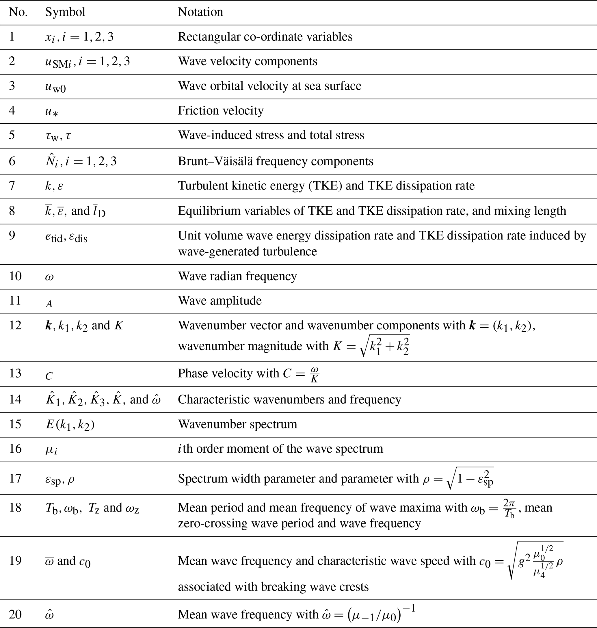
As this study relies heavily on mathematical expressions, a list of symbols is provided in Table D1.

Table D1 Variable notation.