Quantifying farmed kelp atmospheric CO₂ uptake and release through localized air-sea flux measurements in the Northern Gulf of Alaska

The rapid growth of mariculture in the United States, particularly in Alaska, has ignited interest in the co-benefit of using farmed kelp as a mitigation strategy against anthropogenic carbon dioxide (CO₂) released to the atmosphere. Here, we quantified the air-sea CO₂ flux in two kelp farms in the Northern Gulf of Alaska with differing oceanographic conditions and farming practices to determine the carbon sequestration potential over the growing season. Sensors were deployed on two subsurface moorings placed in proximity of one another at each farm site: one “inside” and one “outside” as a reference upstream of the farm. Both sensor arrays conducted hourly measurements of pH or partial pressure of CO₂ (pCO₂), temperature, salinity, and oxygen during the time from seed line outplanting in winter (November to January) to spring harvest (April or May) in 2024. In Windy Bay, nominal differences in carbonate chemistry parameters were detected between the inside and outside moorings from November until March, at which time seawaterpCO₂ within the farm decreased with respect to the reference site. In Kalsin Bay, the inside mooring displayed winter seawater pCO₂ values 100 µatm greater than those recorded at the outside mooring, likely due to the colonization of a biofilm on the kelp lines while young sporophytes were not yet mature; however, seawater pCO₂ values at both moorings converged in spring. Integrated over the entire deployment, one farm strengthened the bay's carbon influx and one farm reversed the natural sink by releasing carbon over the deployment period: 800.1 ± 145.8 mol m⁻² in Kalsin Bay and $-\mathrm{9.23}\pm \mathrm{3.6}$ mol m⁻² in Windy Bay. This study highlights the nuance of farmed kelp carbon capture by demonstrating that a farm site can influence overall air-sea CO₂ flux, whereby farming structures create artificial habitat and that kelp farms are not always a net sink for atmospheric carbon.

1 Introduction

Since the Industrial Revolution, the global ocean has absorbed almost one-third of anthropogenically produced CO₂ (Feely et al., 2004; Quéré et al., 2018), driving a process termed ocean acidification. OA has direct and indirect deleterious effects on marine organisms, such as shell dissolution in crustaceans and mollusks (Ries et al., 2016), malfunctioning olfactory responses in salmon (Williams et al., 2019), and stunted growth and development across trophic levels (Kurihara et al., 2013; Bignami et al., 2013; Long et al., 2013; Alcantar et al., 2024). To help curtail the impacts of these climatic changes, efforts to sequester carbon in ocean environments have been proposed and referred to as marine carbon dioxide removal (mCDR). mCDR methods aim to enhance the flux of CO₂ into the ocean through techniques such as ocean fertilization, ocean alkalinization enhancement, artificial upwelling, and kelp carbon sequestration (DeAngelo et al., 2023; Oschlies et al., 2025).

The burial of biomass from highly productive organisms, such as seaweed, has shown promise as a sustainable option for capturing carbon through enhanced photosynthesis (Jiang et al., 2013; Ikawa and Oechel, 2015). Many kelp farms around the world have demonstrated that atmospheric CO₂ can be taken up by kelp and converted into seaweed biomass (Ikawa and Oechel, 2015; Jiang et al., 2015; Mongin et al., 2016). In Lidao town, China, a kelp farm exhibited variation in net autotrophic activity throughout the year, with the greatest drawdown of atmospheric CO₂ in spring and the least amount in summer (Jiang et al., 2013). However, to achieve climate benefits, kelp farming would need to expand significantly, covering over 90 000 km² (Coleman et al., 2022; DeAngelo et al., 2023). What's more, aging kelp can become a strong net source of dissolved inorganic carbon relative to early stages of kelp, thus restricting the length of time a farm can actively draw down atmospheric CO₂ (Xiong et al., 2024). Given the scale and complication of such efforts, other, more logistically feasible approaches have been proposed, such as implementing the use of kelp farms to locally reduce atmospheric CO₂ concentrations by shifting the magnitude and timing of carbon cycling and providing local refugia from OA (Bednaršek et al., 2024). However, there are negative effects to consider when increasing the footprint of kelp farms as well, such as the reduction of marine recreational access, hazards to navigation, and the removal of nutrients when the kelp biomass is harvested from the water (National Academy of Sciences, Engineering, and Medicine, 2022).

The Northern Gulf of Alaska (NGA) has been identified as a potential site for scaling up kelp farming due to its vast coastline, highly productive waters, and the need to help transition the state economy away from heavy reliance on fossil fuel extraction and unpredictable wild fish stocks (Miller, 2021; Bullen et al., 2024; Edgar et al., 2024). As a result, the NGA kelp farming industry expects to expand dramatically in the next two decades, increasing sustainable economic practices in the state with the added benefit of enabling the Alaskan coastal system and adjoining federal waters to potentially take up atmospheric CO₂ and buffer seawater carbonate chemistry. Local remediation of OA conditions could improve regional mariculture efforts through the co-culturing of shellfish with kelp, with the added benefit of farmed shellfish utilizing macroalgae detritus as a food source (Ries et al., 2016; Haag et al., 2025, 2026). Empirical rate estimates of CO₂ drawdown by kelp from other regions are not universally applicable due to the site-specific interaction of many physical and biological factors that affect kelp-related CO₂ flux rates (Ikawa and Oechel, 2015; Jiang et al., 2015; Mongin et al., 2016). Accordingly, Alaska-specific values are needed to better assess the climate and local benefits of kelp farming in the NGA.

In the NGA, seeded lines are deployed between October and January, and harvested in late spring before biofouling by epiphytic organisms (Stekoll et al., 2021). Coastal marine ecosystems in the NGA are generally net heterotrophic, aside from approximately sixty days of net autotrophy in summer and early fall (Miller and Kelley, 2021); however, on the continental shelf, the ocean acts primarily as a carbon sink (Evans and Mathis, 2013). Currently, there are no estimates of kelp farm air-sea CO₂ fluxes in the NGA, although nearshore macroalgal-dominated habitats can alter carbonate chemistry and create seasonal, localized carbon sinks (Miller and Kelley, 2021). This study quantified the air-sea CO₂ flux in two kelp farms in the NGA to determine the capacity of farmed kelp to take up CO₂ relative to adjacent waters. This study provides empirical estimates of kelp farm-related CO₂ flux, thus exploring the role that Alaska's kelp farming industry can play in reducing atmospheric CO₂ and highlighting the capacity of farms to provide refugia to marine species vulnerable to OA.

2 Materials and methods

2.1 Site descriptions

Two nearshore kelp farms were selected from the Northern Gulf of Alaska (NGA), spanning a distance of 400 km: Royal Ocean Kelp Co in Windy Bay (60.5628° N, 145.9569° W) and Alaska Ocean Farms in Kalsin Bay (57.6581° N, 152.4201° W) (Fig. 1). The two farm sites varied in size, harvest period, and species grown. Alaska Ocean Farms in Kalsin Bay, in operation for three years, covered 3200 m² and grew only Alaria marginata. Seed lines were outplanted in January and harvested in late May. The depth of the site varied from 9 to 18 m, with a tidal range of up to 3 m. The substrate was largely composed of sand. Royal Ocean Kelp Co in Windy Bay covered 12 000 m² and contained two catenary arrays: one of Saccharina latissima and one of A. marginata suspended at approximately 2.2 and 1.2 m depth, respectively. The eight lines making up each array were spaced 3 m apart. Seed lines were outplanted in October and harvested in early May. The water column depth at the farm varied from 12 to 22 m, with a tidal range of 5.5 m. The substrate was largely made up of mud. Neither site is glacially influenced.

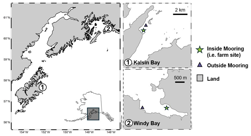
Figure 1 Map of the two kelp farm study sites: Alaska Ocean Farms in Kalsin Bay and Royal Ocean Kelp Co. in Windy Bay. An “inside mooring” was deployed within the farm and an “outside mooring” was deployed upstream of the farm to act as a reference for background respiration and photosynthesis. The distance between these moorings was 100 m in Kalsin Bay and 600 m in Windy Bay. All arrays were suspended 3 m below the surface, roughly the depth of the growing kelp.

2.2 Sensor deployments, calibrations, and carbonate system calculations

A sensor array was deployed inside and outside of each farm (Fig. 1). To estimate net integrated air-sea CO₂ flux of kelp farms through the growing season, the outside mooring must be influenced by the same water mass as the farm to capture background photosynthesis and respiration. In general, the “inside” sensor array was positioned as close to the center of the farm as possible and supported by a buoy. The “outside” sensor array was placed on a mooring a distance from the farm to ensure that it was not influenced by the biological activity of the farm, while still experiencing the same water masses (Fig. 1). Given the different bathymetric and hydrologic features at each farm site, placement distance between the arrays varied; however, the depth of both the inside and outside mooring within the water column were similar across sites. Each sensor array was outfitted with a PME miniDOT optical oxygen logger, an Onset HOBO conductivity logger, a Sea-Bird SeapHOx™ (combination of the SeaFET™ pH sensor and the SBE 37-SMP-ODO MicroCAT CTD+DO sensor) in Windy Bay, and a Sunburst SAMI-CO2™ in Kalsin Bay. The sensor arrays were suspended roughly 3 m from the surface, which is the same depth as the growing kelp, which may misrepresent the flux in highly stratified settings. However, NGA bays experience well-mixed water columns due to strong tidal mixing (Haag et al., 2023), indicating that in locations without strong freshwater input, a sensor placed at 3 m depth would be representative of the near surface. All parameters were measured on a frequency of one hour.

Calibration and reference seawater bottle samples were collected by farmers when they visited their farms by lowering a Science First™ 1.5 L Water Sampler to the depth of the sensor array and filling 250 mL borosilicate bottles pre-spiked with 200 µL saturated mercuric chloride (see Table A1 in the Appendix for anomalies of reference samples relative to sensor values). During the retrieval of the sensors at each site in spring/summer, a survey was conducted to capture within-farm spatial variability in carbonate chemistry by collecting water samples in a grid formation at the depth of the kelp, using the same methods as above. The discrete bottle samples were analyzed for pH_T (total scale) if complementing the pH sensors or dissolved inorganic carbon (DIC) if complementing the CO₂ sensors, and all samples were analyzed for total alkalinity (TA) and salinity. A Shimadzu 1800 spectrophotometer was used to measure seawater pH_T using meta-cresol purple as an indicator dye (Acros, batch #30AXM-QN) and applying a dye impurity correction factor (Douglas and Byrne, 2017). A DIC Analyzer (Apollo SciTech, Model AS-C6L) coupled to a LI-7815 CO₂/H₂O Analyzer measured DIC as well as three different volumes of Certified Reference Material (CRM: Batch 172, A.G. Dickson, Scripps Institute of Oceanography) to create a standard curve with which to calibrate the instrument, as it may drift over time. A Metrohm 848 Titrino plus measured TA via an open-cell titration using a CRM to later calculate sample uncertainty, and a YSI 3100 Conductivity instrument measured salinity.

The SeaFETs were calibrated using the pH_T measured from the discrete seawater samples by calculating electrode-specific single-point calibration coefficients, which were then used to derive the entire pH dataset (Bresnahan et al., 2014; Miller et al., 2018). The HOBO loggers were calibrated with the HOBOware^® Pro software using the salinity and temperature measured by either the CTD within the SeapHOx or temperature-corrected salinity measured within the discrete bottle samples at the lab and temperature recorded by the SAMI-CO₂. The miniDOTs were calibrated using the mean atmospheric pressure and salinity over the deployment. Data can be accessed from the DataONE repository (https://doi.org/10.24431/rw1k9hb, Haag and Kelley, 2025).

Calculations were conducted in R (version 4.4.1) and MATLAB (version R2024b). The uncertainty associated with the pH_T timeseries was calculated following Bresnahan et al. (2014) and Miller and Kelley (2021). In short, the propagated uncertainty incorporated all sources of possible error in the sample analysis procedure: the difference in the lab measurement of pH_T and TA on a known CRM bottle versus the expected values, the constants error for the CO2Sys conversions (following Orr et al., 2018; version 2.3), and the standard deviation of the duplicate calibration bottle measurements (Lewis and Wallace, 1998). Total uncertainty was calculated by adding the propagated uncertainty to the difference between a reference bottle and the calibrated pH timeseries (following Miller and Kelley, 2021). The pH uncertainty was then converted to an in-situ partial pressure of CO₂ (pCO₂) uncertainty using a Monte Carlo simulation, whereby the pH uncertainty was used to create a series of perturbed pH values for each timepoint (n = 10 000) that were then converted to pCO₂ using the “seacarb” package in R (version 3.3.3; Gattuso et al., 2015). When summarizing the timeseries data and spatial survey to single means, the standard deviation was reported to capture the natural variability of the value and not the total uncertainty.

The “seacarb” package can estimate any carbonate system parameters using two known values. The calibrated pH timeseries was used in Windy Bay as the first variable and TA was the second variable calculated from salinity using a known salinity-TA relationship for the nearshore of the NGA (TA = 48.7709 ⋅ S + 606.23 µmol kg⁻¹; Evans et al., 2015; see Fig. A1 in the Appendix), while pCO₂ was directly measured in Kalsin Bay for air-sea flux estimates (Eq. A1 in the Appendix). However, the decomposition analysis required a TA estimation for Kalsin Bay, and the Evans et al. (2015) relationship is not a good proxy for this location based on a sensitivity analysis adapted from Fassbender et al. (2017) (see Appendix). A site-specific salinity-TA equation was estimated using a linear model for this purpose (Fig. A1). The pCO₂ timeseries were subsequently used to calculate air-sea CO₂ fluxes (FCO₂) following Eq. (1) by Wanninkhof (2014):

$$\begin{array}{}\text{(1)}& {\mathrm{FCO}}_{\mathrm{2}}=\mathrm{0.251}{U}^{\mathrm{2}}(\mathit{Sc}/\mathrm{660}{)}^{-\mathrm{0.5}}{K}_{\mathrm{0}}(p{\mathrm{CO}}_{\mathrm{2}\mathrm{w}}-p{\mathrm{CO}}_{\mathrm{2}\mathrm{a}}),\end{array}$$

where U is the wind speed in m s⁻¹, $\mathit{Sc}/\mathrm{660}$ is the dimensionless Schmidt number, K₀ is the Bunsen solubility coefficient with units of mol L⁻¹ atm⁻¹, and pCO_2w and pCO_2a are the pCO₂ in water and air, respectively. Site-specific wind data was obtained from the nearest NDBC buoy to the farm site: Station CRVA2 for Windy Bay located 7 km from the farm and Station KDAA2 for Kalsin Bay located 8 km from the farm (NOAA National Buoy Data Center, 2024; Fig. A2). The near-surface winds at the farm may differ from the wind speed detected at the buoys, therefore giving first-order estimates of the exchange rates rather than precise local fluxes. pCO_2a was assumed to be ∼ 421.2 ppm at all sites (McKain et al., 2024). $\mathit{Sc}/\mathrm{600}$ and K₀ were calculated using the polynomial equations in Wanninkhof (2014). In the absence of wind, the above equation becomes simplified as per MacIntyre (1995) to:

$$\begin{array}{}\text{(2)}& {\mathrm{FCO}}_{\mathrm{2}}=\mathrm{0.8}{K}_{\mathrm{0}}(p{\mathrm{CO}}_{\mathrm{2}\mathrm{w}}-p{\mathrm{CO}}_{\mathrm{2}\mathrm{a}}),\end{array}$$

since atmospheric exchange continues even when turbulent mixing at the water surface does not occur. The net integrated FCO₂, a measure of the kelp farm effect, was calculated by subtracting the FCO₂ estimated for the inside mooring from the outside mooring for each farm site location and integrating over the entire timeseries. An uncertainty for total net integrated FCO₂ was calculated by propagating the errors associated with each of the sensors and the data pulled from online resources through the air-sea flux calculation and integration.

Since there is no established SAMI-CO2™ sensor post-calibration method – outside that from the manufacturer – we utilized an independent cross-validation approach to assess SAMI-CO2™ data integrity. We conducted a stoichiometric cross-validation using hourly O₂ data from co-located miniDOT sensors. Assuming a 1 : 1 stoichiometry (O₂ : DIC), we calculated O₂-derived expected pCO₂ and compared that to the measured time series. The relationship between measured and expected pCO₂ was evaluated using Pearson's correlation and ordinary least squares linear regression.

2.3 Ancillary data analysis

Temperature-salinity (T-S) diagrams were used to determine if the inside and outside moorings experienced the same water mass, since a water mass can be defined by their salinity and potential temperature, as those variables remain conserved unless experiencing mixing conditions or processes such as evaporation/precipitation and air-sea heat fluxes that should be negligible at small scales such as the distance between moorings. T-S diagrams were created by modifying the “ggTS” function (Kaiser, 2020), which utilized the “gsw” package to calculate the potential density and plot isopycnals (version 1.2-0; Kelley et al., 2024). Similarities between the T-S diagrams for both moorings would indicate that the outside mooring can act as a reference for the inside mooring. The lag time of the water mass between the outside and inside moorings was characterized by detrending the data and applying a cross-correlation using the “tseries” package (version 0.10-58; Trapletti et al., 2015).

The timeseries at each site was divided into two phases in order to compare carbonate chemistry shifts throughout the kelp growing season: heterotrophy and autotrophy. Net heterotrophy or autotrophy of seawater was determined by calculating the apparent oxygen production (AOP) across the timeseries, which is the difference between the measured in-situ oxygen versus the estimated oxygen saturation as a function of temperature and salinity (Garcia and Gordon, 1992: equations corrected from Casamitjana and Roget, 1993). The shift from net heterotrophy to net autotrophy in spring was estimated as the minimum of the cumulative sum of AOP measured at the outside mooring.

The drivers of seawater pCO₂ were assessed by doing a decomposition of monthly averages of pCO₂ based on the effects of temperature (T), salinity (S), total alkalinity (TA), air-sea CO₂ flux (FCO₂), and dissolved inorganic carbon (DIC). The following equations were modified from García-Troche et al. (2021), originally based on pH, to describe observed hourly changes between two consecutive hours (t₁ and t₂):

$$\begin{array}{}\text{(3)}& \begin{array}{rl}\mathrm{\Delta }p{\mathrm{CO}}_{\mathrm{2}}& =\mathrm{\Delta }p{\mathrm{CO}}_{\mathrm{2}}\left(T\right)+\mathrm{\Delta }p{\mathrm{CO}}_{\mathrm{2}}\left(S\right)+\mathrm{\Delta }p{\mathrm{CO}}_{\mathrm{2}}\left(\mathrm{TA}\right)\\ & +\mathrm{\Delta }p{\mathrm{CO}}_{\mathrm{2}}\left({\mathrm{FCO}}_{\mathrm{2}}\right)+\mathrm{\Delta }p{\mathrm{CO}}_{\mathrm{2}}\left(\mathrm{DIC}\right)+R,\end{array}\end{array}$$

where a change in seawater pCO₂ from one hour to another (ΔpCO₂) can be described as the changes to the five variables plus a residual (R), which represents any remaining ΔpCO₂ not explained by T, S, TA, FCO₂, or DIC. Using the “seacarb” package in R, the stepwise calculated change in pCO₂ between t₁ and t₂ was derived by a single variable at a time to calculate the hourly ΔpCO₂(T), ΔpCO₂(S), and ΔpCO₂(TA):

$$\begin{array}{}\text{(4)}& {\displaystyle }\mathrm{\Delta }p{\mathrm{CO}}_{\mathrm{2}}\left(T\right)=\mathrm{\Delta }p{\mathrm{CO}}_{\mathrm{2},\mathrm{2}}\left(T_{\mathrm{2}},S_{\mathrm{1}},{\mathrm{TA}}_{\mathrm{1}},{\mathrm{DIC}}_{\mathrm{1}}\right)-\mathrm{\Delta }p{\mathrm{CO}}_{\mathrm{2},\mathrm{1}},\text{(5)}& {\displaystyle }\mathrm{\Delta }p{\mathrm{CO}}_{\mathrm{2}}\left(S\right)=\mathrm{\Delta }p{\mathrm{CO}}_{\mathrm{2},\mathrm{2}}\left(T_{\mathrm{1}},S_{\mathrm{2}},{\mathrm{TA}}_{\mathrm{1}},{\mathrm{DIC}}_{\mathrm{1}}\right)-\mathrm{\Delta }p{\mathrm{CO}}_{\mathrm{2},\mathrm{1}},\text{(6)}& {\displaystyle }\mathrm{\Delta }p{\mathrm{CO}}_{\mathrm{2}}\left(\mathrm{TA}\right)=\mathrm{\Delta }p{\mathrm{CO}}_{\mathrm{2},\mathrm{2}}\left(T_{\mathrm{1}},S_{\mathrm{1}},{\mathrm{TA}}_{\mathrm{3}},{\mathrm{DIC}}_{\mathrm{1}}\right)-\mathrm{\Delta }p{\mathrm{CO}}_{\mathrm{2},\mathrm{1}},\end{array}$$

Due to DIC exerting an effect on both ΔpCO₂(FCO₂) and ΔpCO₂(DIC), as a result of air-sea CO₂ exchange and water column/benthic processes, respectively, ΔpCO₂(FCO₂) was calculated first and subsequently used to separate its signal from ΔpCO₂(DIC). ΔpCO₂(FCO₂) required an estimate of hourly CO₂ air-sea exchange calculated using Eqs. (1) and (2) (i.e., FCO₂), the change in time (t₂−t₁, h), seawater density (d, kg m⁻³), and water column height (H, m) from García-Troche et al. (2021):

$$\begin{array}{}\text{(7)}& {\displaystyle }\mathrm{\Delta }{\mathrm{DIC}}_{\mathrm{air}-\mathrm{sea}}={\displaystyle \frac{-{\mathrm{FCO}}_{\mathrm{2}}\times (t_{\mathrm{1}}-t_{\mathrm{2}})}{d\times H}},\text{(8)}& {\displaystyle }\begin{array}{rl}\mathrm{\Delta }p{\mathrm{CO}}_{\mathrm{2}}\left({\mathrm{FCO}}_{\mathrm{2}}\right)& =\mathrm{\Delta }p{\mathrm{CO}}_{\mathrm{2},\mathrm{2}}(T_{\mathrm{1}},S_{\mathrm{1}},{\mathrm{TA}}_{\mathrm{1}},{\mathrm{DIC}}_{\mathrm{1}}\\ & +\mathrm{\Delta }{\mathrm{DIC}}_{\mathrm{air}-\mathrm{sea},\mathrm{2}})-\mathrm{\Delta }p{\mathrm{CO}}_{\mathrm{2},\mathrm{1}},\end{array}\text{(9)}& {\displaystyle }\begin{array}{rl}\mathrm{\Delta }p{\mathrm{CO}}_{\mathrm{2}}\left(\mathrm{DIC}\right)& =\mathrm{\Delta }p{\mathrm{CO}}_{\mathrm{2},\mathrm{2}}\left(T_{\mathrm{1}},S_{\mathrm{1}},{\mathrm{TA}}_{\mathrm{1}},{\mathrm{DIC}}_{\mathrm{2}}\right)\\ & -\mathrm{\Delta }p{\mathrm{CO}}_{\mathrm{2}}\left({\mathrm{FCO}}_{\mathrm{2}}\right)-\mathrm{\Delta }p{\mathrm{CO}}_{\mathrm{2},\mathrm{1}},\end{array}\end{array}$$

The monthly periodicity of pCO₂ was estimated with a power spectral analysis using R package “spectrum” (version 1.1; John and Watson, 2020). The span was set to 20 d. A high-pass Butterworth filter (package “signal”; version 1.8-1; Ligges et al., 2015) was first applied to remove low-frequency components that can dominate the spectrum. The cutoff was set to 0.01 cycles h⁻¹. The underlying periodicities were plotted to visually determine the dominant drivers of pH_T frequency.

3 Results

3.1 Comparison of inside and outside moorings

Comparison of water mass movement at the inside and outside moorings confirmed that both sensor arrays detected similar water masses, permitting the calculation of net integrated air-sea CO₂ flux. T-S diagrams were remarkably similar between inside and outside moorings across sites, with distinct shifts through time driven by temperature, denoted in the colour overlay (Fig. 2). Salinity remained relatively consistent through the deployment period (30.0 ± 0.6 in Kalsin Bay and 31.1 ± 0.4 in Windy Bay) while temperature at both sites decreased from winter to early spring before warming once again (Fig. 2). The inflection of temperature warming occurred at different times depending on the site: mid-March in Kalsin Bay and mid-April in Windy Bay. The within-site cross-correlations measured between salinity and temperature indicated a lag time of 1 h according to salinity and 0 h according to temperature in Kalsin Bay, and 1 h in Windy Bay for both variables, underscoring the strong similarities between water masses at the inside and outside moorings.

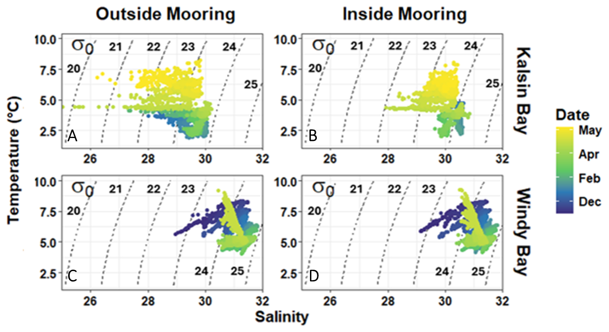
Figure 2 Temperature-salinity diagrams from two locations in the Northern Gulf of Alaska at moorings within kelp farms (inside moorings; B, D) and reference moorings upstream of the farm sites (outside moorings; A, C). Sensor arrays collected hourly data from 3 m depth. Labelled dashed lines denote isolines of potential density anomaly (σ_θ; −1000 kg m⁻³).

Apparent oxygen production (AOP), the difference between in-situ O₂ and O₂ saturation estimated as a function of temperature and salinity, indicated that both nearshore systems experienced a distinct shift from net heterotrophy to net autotrophy throughout the growing season (Fig. 3). Both sites experienced wintertime net heterotrophy until early spring when AOP neared the solubility compensation point (AOP = 0) and transitioned into net heterotrophy (on 12 February in Kalsin Bay and 19 March in Windy Bay). At both sites, the inside mooring was characterized by higher net autotrophy than the outside mooring as time neared harvest (Fig. 3).

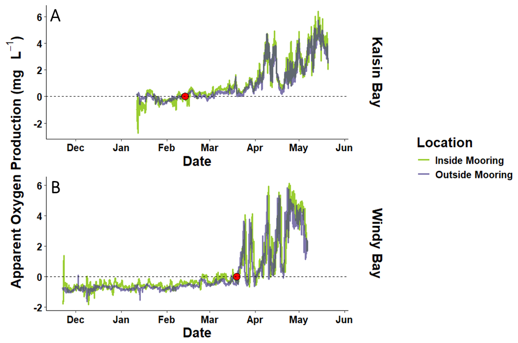
Figure 3 Apparent oxygen production (i.e., measured O₂ minus saturated O₂) across the farmed kelp growing season and the following summer in Kalsin Bay (A) and Windy Bay (B) both inside the farm (inside mooring) and at the reference site outside of the farm (outside mooring). The dashed line indicates when measured O₂ is equal saturated O₂ and thus denotes the solubility compensation point. The red dots indicate the transition from net heterotrophy to net autotrophy in spring.

During the period of net heterotrophy in winter, both timeseries measured outside of the farm displayed seawater pCO₂ values greater than atmospheric CO₂ (i.e. 421.2 µatm; McKain et al., 2024; Fig. 4). In Windy Bay, the inside and outside moorings had associated total uncertainties of 69.46 and 73.73 µatm, respectively. The average pCO₂ at the outside mooring during this wintertime net heterotrophic period was 453.8 ± 15.0 µatm (n=750) in Kalsin Bay and 482.2 ± 22.4 µatm (n=2840) in Windy Bay. During the period of net autotrophy in spring, seawater pCO₂ decreased below atmospheric CO₂ at both sites, with a concurrent increase in pCO₂ variability (Fig. 4). The average pCO₂ at the outside mooring during this time was 326.5 ± 94.1 µatm (n=2336) for Kalsin Bay and 308.1 ± 100.4 µatm for Windy Bay (n=1159). The stoichiometric cross-validation of the SAMI-CO2™ sensor using the miniDOT oxygen sensor for Kalsin Bay confirmed high data integrity, with measured pCO₂ exhibiting exceptionally strong, positive linear correlations with O₂-derived expected pCO₂ at both the inside (Pearson's r = 0.95, p<0.001) and outside (Pearson's r = 0.95, p < 0.001) moorings. Regression analysis indicated that biological forcing explained approximately 90 % of the observedpCO₂ variance (R² = 0.90) at Kalsin Bay (Fig. A3).

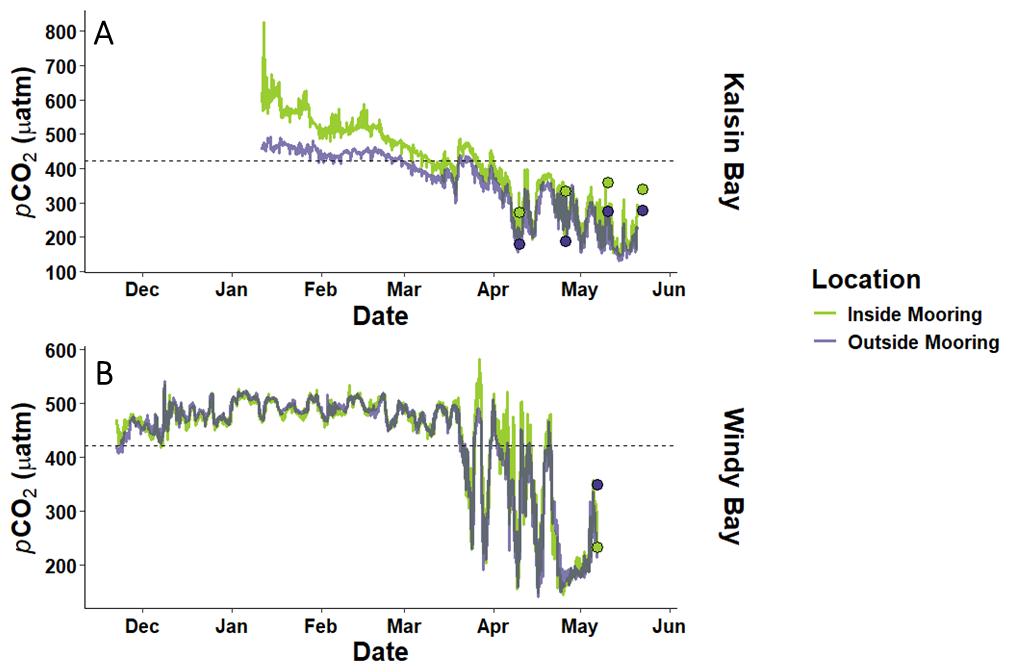
Figure 4 The partial pressure of carbon dioxide (pCO₂) in seawater inside and outside of kelp farms across the kelp growing season in Kalsin Bay (A) and Windy Bay (B). The dashed line indicates the atmospheric CO₂ value, which has been estimated to be ∼ 421.2 ppm at all sites (McKain et al., 2024). The dots indicate reference samples collected at both the inside (green) and outside (purple) moorings.

3.2 Air-sea CO₂ flux timeseries

Air-sea CO₂ flux estimations (FCO₂) for all sites and moorings demonstrated a flux of CO₂ from the ocean to the atmosphere during the net heterotrophic period indicated by AOP (Figs. 3; 5). The FCO₂ for the outside mooring during net heterotrophy ranged between −0.002 to 0.676 mmol m² h⁻¹ in Kalsin Bay (0.049 ± 0.081 mmol m² h⁻¹, n = 750) and −0.069 to 1.253 mmol m² h⁻¹ in Windy Bay (0.057 ± 0.111 mmol m² h⁻¹, n = 2840). As the period of net heterotrophy ended, both sites became carbon sinks. The proportional difference in FCO₂ between moorings (i.e., the FCO₂ at the inside mooring divided by the outside mooring) increased at both sites over time (see Fig. A4), demonstrating that as the kelp growing season progressed, so did the difference in FCO₂ estimated at the paired moorings. FCO₂ at the outside mooring ranged between −1.83 to 0.314 mmol m² h⁻¹ in Kalsin Bay (−0.081 ± 0.174 mmol m² d⁻¹, n = 2336) and −1.016 to 0.456 mmol m² h⁻¹ in Windy Bay (−0.046 ± 0.116 mmol m² h⁻¹, n = 1159).

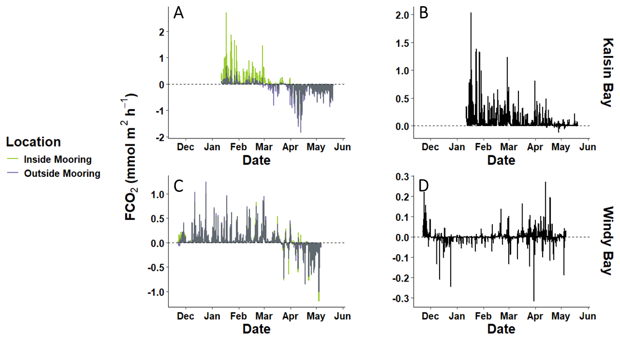
Figure 5 The partial variation in air-sea CO₂ fluxes (FCO₂) across the kelp growing season at two different sites (A, C) and the net integrated FCO₂ representing the inside versus the outside fluxes integrated over time sensor deployment (B, D).

The influence of the kelp farms strengthened the carbon sink at Windy Bay but reversed the carbon sink to a carbon source at Kalsin Bay (Fig. 5). Net FCO₂, the difference in FCO₂ at the inside versus outside moorings representing the farm signal, integrated from the start of the kelp outplanting (Fig. 2) to harvest, was 800.1 ± 145.8 mmol m⁻² in Kalsin Bay and −9.2 ± 3.6 mol m⁻² in Windy Bay. The small net negative integrated FCO₂ in Windy Bay was due to equal variation in FCO₂ above and below zero throughout the sensor deployment (Fig. 5). The net integrated FCO₂ across the timeseries was within the same magnitude as those of the outside mooring, indicating that large differences were experienced at the inside and outside moorings of both sites.

The inside mooring value corresponded with the spatial samples collected at Kalsin Bay at the time of kelp harvest, while the mooring underestimated the FCO₂ of the farm spatial sampling at Windy Bay (Fig. 6). The spatial surveys at each farm indicated a FCO₂ of −0.150 ± 0.183 mmol m² h⁻¹ at Kalsin Bay (n = 8), and 0.049 ± 0.007 mmol m² h⁻¹ at Windy Bay (n = 9). The FCO₂ of the sample collected at the outside mooring exceeded the farm samples in Windy Bay but was lower at Kalsin Bay (Fig. 6). The FCO₂ estimate from the timeseries mooring in Kalsin Bay was within the spread of samples measured discretely at the farm, though one of the discrete bottle samples in the farm was comparable to the outside farm sample (Fig. 6). In Windy Bay, mooring values fell below the range measured discretely at the farm (Fig. 6). This spatial survey demonstrated the homogeneity of FCO₂ at the farm and discrepancy between the mooring timeseries and discrete bottle sample FCO₂.

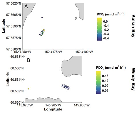
Figure 6 The spatial variation in air-sea CO₂ fluxes (FCO₂) across a kelp farm (denoted by the shaded rectangle) at two different sites directly before harvest: 22 May in Kalsin Bay (n = 9; A) and 6 May in Windy Bay (n=10; B). The point outside the shaded rectangle denotes the value at the outside mooring.

3.3 Drivers of seawater pCO₂

The seawater pCO₂ decomposition demonstrated that hourly changes to pCO₂ were influenced primarily by biological processes and air-sea flux, as both ΔpCO₂(DIC) and ΔpCO₂(FCO₂) exerted the most considerable change in pCO₂ (Fig. 7). DIC and FCO₂ applied both positive and negative changes to pCO₂ depending on site and time during the kelp growing season, but always as opposing forces. Salinity and temperature played a negligible role in ΔpCO₂ both sites during all months (Fig. 7). Therefore, the concentration of DIC in seawater, controlled primarily by biological processes, and the hourly air-sea CO₂ flux drove the changes in seawater pCO₂. The five drivers used to decompose the hourly changes in seawater pCO₂ included all major sources of variability in Kalsin Bay but not Windy Bay. In Kalsin Bay, the remaining residuals ranged between −3.8 to 1.04 µatm ($-\mathrm{0.01}\pm \mathrm{0.14}$ µatm, n=3086) at the inside mooring and −13.2 to 2.6 µatm ($-\mathrm{0.04}\pm \mathrm{0.33}$ µatm, n = 3086) at the outside mooring. In Windy Bay, the remaining residuals ranged between −44.5 to 2.4 µatm ($-\mathrm{0.3}\pm \mathrm{1.6}$ µatm, n=3997) at the inside mooring and −41.5 to 0.7 µatm ($-\mathrm{0.3}\pm \mathrm{1.5}$ µatm, n=3997) at the outside mooring. These residuals suggest that an additional moderate source of seawater pCO₂ was present in Windy Bay but not included as a parameter and was not captured in the decomposition analysis.

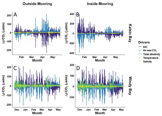
Figure 7 Hourly changes in pCO₂ due to temperature, salinity, air-sea CO₂ flux, total alkalinity, and dissolved inorganic carbon at Kalsin Bay (A, B) and at Windy Bay (C, D) at a mooring inside the kelp farm (B, D) and a reference site upstream (A, C).

The power spectral density (PSD) analysis revealed distinct site-specific and monthly differences in seawater pCO₂ periodicity that suggest diel and tidal cycling to be important drivers, particularly as spring progresses (Fig. 8). Frequencies observed at 2 d⁻¹ correspond to 12 h cycles, likely driven by tidal forcing. This frequency was apparent in Windy Bay (Fig. 8), suggesting that tides play a role in pCO₂ variability in Windy Bay but not Kalsin Bay. Frequencies corresponding to 1 d⁻¹, observed at all sites, indicate a diel periodicity. The most likely driver of a diel cycle would be irradiance. Although temperature and salinity may change as a product of the day/night cycle, the decomposition of pCO₂ indicated that these factors played minimal roles in controlling seawater pCO₂ (Fig. 7). There were multiple peaks <1 d⁻¹: 0.3 in Kalsin Bay, and 0.3 and 0.6 in Windy Bay. Frequencies at 0.3 and 0.6 d⁻¹ correspond to periodicity in seawater pCO₂ every 3.3 and 1.6 d. Further, the peaks of PSD grew stronger as spring progressed, with observable peaks beginning in April for Kalsin Bay and in March for Windy Bay (Fig. 8).

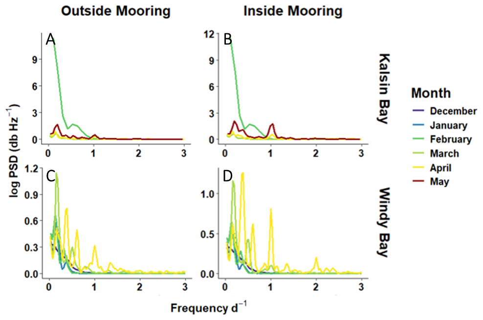
Figure 8 Monthly power spectral density analysis for Kalsin Bay (A, B) and Windy Bay (C, D), inside and outside of the kelp farm at 3 m depth (B, D, and A, C, respectively).

4 Discussion

This study is the first in Alaska to directly measure, at high frequency (hourly), the effect of kelp farming on the seawater carbonate system. Both kelp farms, located in Kalsin Bay and Windy Bay, varied in their magnitude and direction of their influence on nearshore carbon flux. Across the kelp growing season, which extends from winter to spring, Windy Bay demonstrated a net negative integrated air-sea CO₂ flux (i.e., carbon moved from the atmosphere to the ocean), while Kalsin Bay exhibited a net efflux of carbon to the atmosphere (Fig. 5). These differing responses are attributed to biological processes, which disparately modified seawater DIC and the balance between diel cycling of seawater pCO₂ (Figs. 7; 8). This suggests that carbon sequestration potential of kelp farms in the NGA may be site-specific. Results from one site cannot be generalized across the region, highlighting the need for studies that compare CO₂ air-sea flux measurements from multiple sites across a heterogeneous coastal landscape.

4.1 Influence of site-specific differences in air-sea CO₂ fluxes (FCO₂)

Each site differed in its response to apparent oxygen production, pCO₂ concentration, air-sea CO₂ flux (FCO₂), and periodicity, demonstrating the need to determine site-specific influences on kelp farm carbon uptake (Figs. 3; 4; 5; 6; 7; 8). Both sites experienced a shift from net heterotrophy to net autotrophy in spring (Fig. 3). The timing of the shift from heterotrophy to autotrophy coincided with the ocean changing from a carbon source to a carbon sink (Fig. 4). The ∼ 100 µatm pCO₂ gradient observed between Kalsin Bay inside and outside moorings during the winter deployment was initially scrutinized given the short distance between moorings of ∼ 100 m. However, the robust stoichiometric coupling between pCO₂ and O₂ (Fig. A3) confirms that, independently, the SAMI-CO2™ sensor and the miniDOT oxygen sensor were observing biologically driven environmental signals. This high degree of correlation (Fig. 4A; Pearson's r=0.95, p<0.001; R²=0.90 for both moorings) provides confidence that the observed winter differences in measured pCO₂ between moorings represent a real spatial decoupling and are not the result of sensor malfunction or drift. This suggests that the biofilm observed by the farmer on their kelp lines early in the season may have contributed to the elevated pCO₂ values at the inside mooring (A. Pryor, personal communication, 22 May 2024). The respiration of microbial biofilms, and microbial communities in general, have been shown to significantly affect seawater carbonate chemistry (Magalhães et al., 2003). In Kalsin Bay, the presence of the farm structure allowed an opportunity for the colonization of a microbial community that strengthened the ocean's carbon efflux to the atmosphere, creating an artificial habitat of 3200 m². As the nearshore transitioned into a carbon sink in spring (Fig. 5), the pCO₂ at the kelp farm converged with the reference site, but the farm still resulted in a net integrated carbon sink due to that initial wintertime respiration (Fig. 5).

This study cannot differentiate between kelp species or population-level differences. In Windy Bay, both S. latissima and A. marginata were grown, while only A. marginata was grown in Kalsin Bay. Different kelp species exhibit different rates of photosynthesis due to physiology and diverging adaptations to a preferred environment (Van der Loos et al., 2019): S. latissima has adapted to low-light and low-energy environments, while A. marginata has adapted to the high-energy, wave-exposed intertidal. Additionally, intraspecific variation in photosynthetic rates between sites may occur, with regional adaptation to local conditions at these NGA farms that are >300 km apart (Bruhn et al., 2016). The farming gear and methods implemented at a given site may also have caused observable differences in the effect of cultured kelp on seawater carbonate chemistry. This study benefitted from studying two established commercial kelp farms, but the locations differed in farm size, line spacing, and seeded line source, all of which can influence kelp growth (Boderskov et al., 2021; Umanzor et al., 2025). In Kodiak, AK, decreasing the line spacing limited the growth of kelp blades but resulted in higher total yield (Umanzor et al., 2025). Notably, the quality of seeded line produced in hatcheries within the NGA varies significantly as these hatcheries continue to improve production for this nascent industry, and seeding method directly correlates with final yields (Boderskov et al., 2021). The variability of farming techniques across locations, paired with site- and species-specific physiology, makes definitively decomposing the primary drivers of kelp production and subsequent FCO₂ difficult to achieve.

4.2 Drivers of nearshore carbonate chemistry in kelp farms

The short-term periodicity observed in seawater pCO₂ was accounted for by diel and tidal cycling, and therefore a heightened biological signal, but the longer “event-scale” variability observable across all timeseries has not yet been explained (Figs. 4; 7; 8). Across the sites, this variability spanned 1.6 or 3.3 d intervals, with periodicities strengthening in April and May (Fig. 7). Event-scale variability has previously been attributed to phytoplankton blooms, advection of upwelled water, and wind relaxation (Kapsenberg and Hofmann, 2016). Phytoplankton blooms persist on scales of two to three weeks (Eslinger et al., 2001), and wind/air-sea exchange played a minimal role in driving changes in pCO₂ in this study (Fig. 7), so these variables are likely not driving observed periodicity (Fig. 8). Short water residence times in recessed bays in the NGA can cause elevated mixing with offshore water (Haag et al., 2023), and the undersaturated seawater on the continental shelf could act to dilute the inshore pCO₂ with mixing (Evans and Mathis, 2013). This mixing with offshore water might explain the event-scale periodicity and remaining residuals from the decomposition of the monthly changes in seawater pCO₂. Windy Bay, in particular, demonstrated elevated residuals from the pCO₂ decomposition, suggesting that our analysis lacked a critical carbon sink at this site. The greatest difference between Windy Bay and Kalsin Bay is the proximity of Windy Bay to the Copper River, the single largest point source of freshwater in the NGA (Reister et al., 2024). In Kalsin Bay, the high pCO₂/low O₂ event (825 µatm, 7.22 mg L⁻¹, respectively) observed on 12 January 2024 deviated substantially from temporally adjacent observations (Fig. 4). The observed anomaly corresponded to an especially high perigean spring tide event beginning 11 January, with a low tide of −0.58 m, 05:00 UTC 12 January, aligning perfectly with the noted pCO₂ spike. Tidal pumping, a dominant driver of submarine groundwater discharge flux in coastal Alaska (Haag et al., 2023), likely drove this excursion by forcing pCO₂-enriched, oxygen-depleted porewater from the surrounding sediment into the water column during the ebbing tide. Cyronak et al. (2014) noted tidal pumping can be a dominant driver of pCO₂ variability in coastal systems, where the drainage of highpCO₂ groundwater or porewater during spring low tides significantly enhances local pCO₂. While our study is speculative, further research should quantify the relative carbon fluxes in these bays and determine how long the effect of the carbon uptake by kelp persists in these nearshore sites after harvest.

While one of the two kelp farms strengthened the atmospheric drawdown of CO₂ across the growing season, the hourly FCO₂ varied from being a source to a sink of carbon, sometimes within the same twenty-four-hour period (Fig. 5). Coastal oceans exhibit strong diel cycles in pCO₂, and the NGA was not an exception (Fig. 8; Torres et al., 2021). The diel photosynthesis/respiration cycle of primary producers can alter the availability of TA and DIC in seawater and was the dominant driver of pCO₂ in the region such that it could drive both positive and negative FCO₂ should seawater pCO₂ rise above and fall below atmospheric CO₂ (Fig. 7; Torres et al., 2021). Wind speed dominates the magnitude of these fluxes; therefore, an increasing differential between seawater and atmospheric CO₂ would still require strong winds to drive FCO₂ (Eqs. 1 and 2). However, wind forcing weakens through spring, which can slow air-sea CO₂ equilibration (Stabeno et al., 2004). Therefore, the timing of wind and air-sea CO₂ differentials are important when considering the ability of kelp farms to draw down atmospheric CO₂, as a mismatch between seasonal winds and the farmed kelp growing season would result in a reduction of CO₂ uptake (see wind speed in Fig. A2).

4.3 Carbon credit and ocean acidification mitigation

If one were to consider the uptake of carbon from seawater by a kelp farm, with the assumption that the kelp will be removed from the system through harvest, an estimate of carbon credit capacity can be made using the farm dimensions. The FCO₂ within each farm was fairly homogeneous at the timepoint sampled (Fig. 6), further bolstering the notion that the timeseries measured at the mooring was representative of the entire farm. To account for the ability of Alaskan farmed kelps to use CO₂ or bicarbonate as a source of carbon, we calculated the carbon credits two ways: we multiplied both the (1) net integrated dissolved inorganic carbon (DIC) and (2) the net integrated FCO₂ between the inside and outside moorings by the area of the farm, assuming the kelp occupied a conservative 1 m depth in the water column. Over the growing season, this produced an uptake of DIC into kelp tissue of 4289 t CO₂ eq. in Windy Bay and a release of 18 269 t CO₂ eq. in Kalsin Bay, an atmospheric CO₂ drawdown of 4995 t CO₂ eq. in Windy Bay, and an atmospheric CO₂ release of 115 465 t CO₂ eq. in Kalsin Bay. To sell farmed kelp as a carbon credit, farmers would be required to prevent the harvested biomass from being remineralized by sinking their product off the continental shelf in locations of periodic or permanent anoxia (Pedersen et al., 2021; Duarte et al., 2025), or by other means, which would leave the carbon credits as the sole source of income for farmers choosing this route. This method would also remove fixed nutrients from the nearshore system and potentially degrade the marine system (Campbell et al., 2019), especially if the kelp were grown at scale in this region.

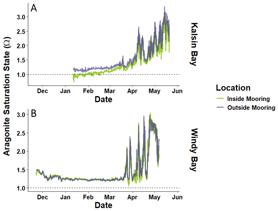
Figure 9 The aragonite saturation in seawater (Ω_arag) inside and outside of kelp farms across the kelp growing season in Kalsin Bay (A) and Windy Bay (B). The dashed line indicates when seawater is at saturation with respect to aragonite (Ω_arag=1).

Kelp farms may also act as local refugia against ocean acidification by creating a halo effect of higher pH water in their vicinity, altering the seawater chemistry so that biocalcification is more favorable (Krause-Jensen et al., 2015; Ries et al., 2016). When aragonite is at saturation with respect to the mineral solubility product in seawater, the aragonite saturation state (Ω_arag) is 1, and seawater Ω_arag remained above that value across most of the NGA, except for within the Kalsin Bay farm in winter (Fig. 9). The presence of kelp farms appeared to reduce the aragonite saturation of seawater in both farms, which may increase the exposure of organisms to conditions favouring dissolution in future OA conditions if the kelp farm were to scale up, especially during brief windows of opportunity when organisms experience sensitive life stages (Ross et al., 2011).

Estimates of other sources and sinks of kelp-derived carbon in the marine environment are needed to contextualize the effect of farmed kelp, particularly the effect of phytoplankton in controlling the seawater carbonate chemistry. There are extended periods of time during summer where farmed kelp is not present, as it is harvested in early spring and not reseeded until the following winter (Stekoll et al., 2021); however, there are no current estimates in the NGA to the residence time of kelp detritus in the water column. To ascertain the role of kelp farms in carbon cycling, further research should seek to quantify the longevity of kelp influence after harvest and natural drivers of carbon in the nearshore. For example, submarine groundwater discharge plays a dominant role in nutrient cycling in southcentral NGA due to the high tidal forcing in the area (Haag et al., 2023) – and tides were also demonstrated to be an important driver of seawater pCO₂ (Fig. 8) – but there are no current estimates for advective carbon fluxes at the sediment-water interface. Future deployments could pair sensor arrays with current profilers to more directly resolve tidal advection dynamics, as this study could not account for the additional uncertainty of tidal reversals and measure chlorophyll to determine the biomass of phytoplankton in the water column.

5 Conclusions

Kelp farms influenced the seawater carbonate chemistry and air-sea CO₂ flux in two bays in the NGA. During the growing season, which extends from winter into late spring, the farmed kelp at one of the farms increased the capacity for the nearshore to act as a CO₂ sink, while the second farm had the opposite effect. A higher capacity of atmospheric carbon drawdown may be attainable at targeted farm sites where kelp farms increase the carbon sink capacity of the ocean if mariculture activities were to scale, though further studies into intraspecific- and interannual variability would be required to actualize a carbon credit market from Alaska's kelp farming industry.

Appendix A

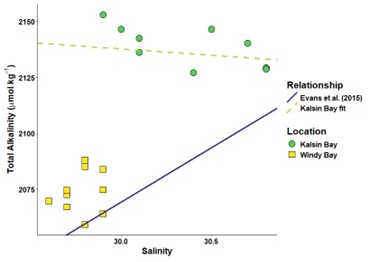
Figure A1 The spread of discrete samples taken at the farm sites at the end of the sensor deployments (22 May in Kalsin Bay and 6 May in Windy Bay) according to their total alkalinity and salinity. Two salinity-temperature relationships are denoted: one devised by Evans et al. (2015) and one created specifically for Kalsin Bay using the displayed discrete samples.

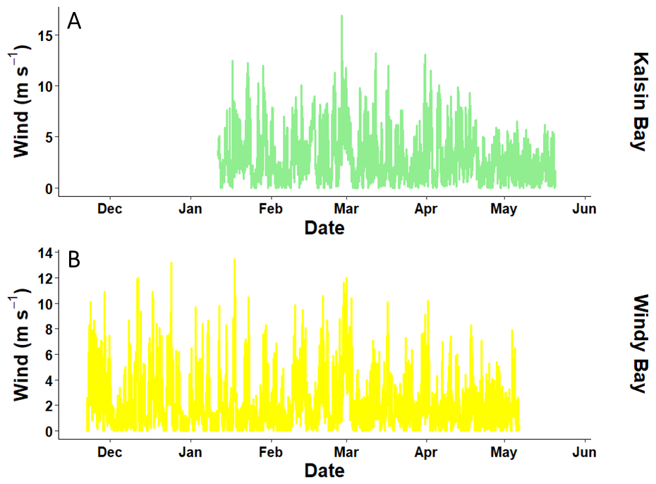
Figure A2 The wind speed measured by NDBC buoys (Station CRVA2 for Windy Bay located 7 km from the farm and Station KDAA2 for Kalsin Bay located 8 km from the farm) used to calculate the air-sea CO₂ flux at the two farm sites.

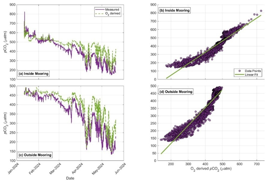
Figure A3 Comparison of autonomous pCO₂ and O₂-derived expected pCO₂ at the Kalsin Bay kelp farm. Panels (a) and (c) display the time-series observations for the inside mooring and outside control mooring, respectively, illustrating the coupled oscillations between dissolved gases. Panels (b) and (d) show the linear regression analysis between measured pCO₂ and O₂-derived expected pCO₂ for the inside and outside sites. Tight stoichiometric coupling (R² ≥ 0.90, p<0.001) across both the kelp farm and the reference site confirms sensor functionality.

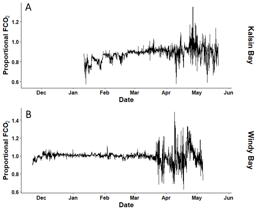
Figure A4 The proportional difference in air-sea CO₂ fluxes (FCO₂) between the inside of a kelp farm relative to ambient conditions at Kalsin Bay (A) and Windy Bay (B) calculated by dividing the inside mooring by the outside mooring.

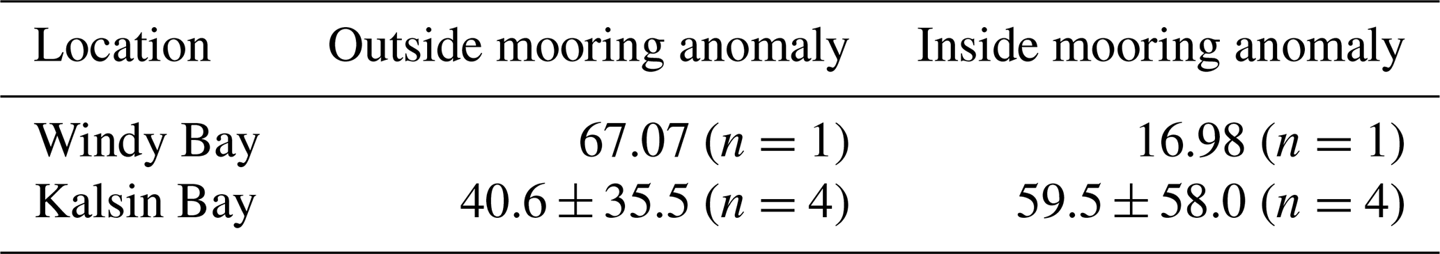
Table A1 The absolute anomalies between sensor-derived pCO₂ and bottle-derived pCO₂ at Kalsin Bay and Windy Bay.

A1 TA-salinity sensitivity analysis

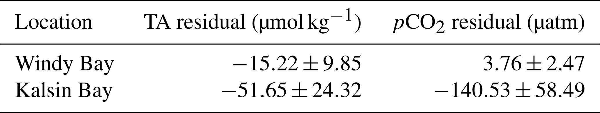
We adapted the methods of Fassbender et al. (2017) to estimate the sensitivity of pCO₂ values derived from predicted total alkalinity (TA) values. The sensor arrays deployed in this study did not measure TA, so we wanted to use a known salinity-TA relationship established by Evans et al. (2015) for the region to estimate a timeseries of TA to then estimate pCO₂ as estimations of the carbonate system require two known variables. We utilized discrete samples measured for TA and one other carbonate chemistry parameter in the lab for this purpose. First, we predicted the TA values for the bottle samples only using salinity and the Evans et al. (2015) relationship. Next, we calculated the residual for the bottle samples' predicted TA and the measured TA. Then, we used the “seacarb” package in R to estimate the pCO₂ for each sample twice, once using the predicted TA and once the measured TA, and compared again the final pCO₂ values for the sensitivity. The results demonstrated that the Evans et al. (2015) relationship would work for one of the two sites only (Table A2).

Table A2 The residuals associated with the difference between the measured total alkalinity and resulting estimated pCO₂ value and a total alkalinity value predicted by Evans et al. (2015) and its resulting estimated pCO₂ value. Values are shown as the mean ± standard deviation.

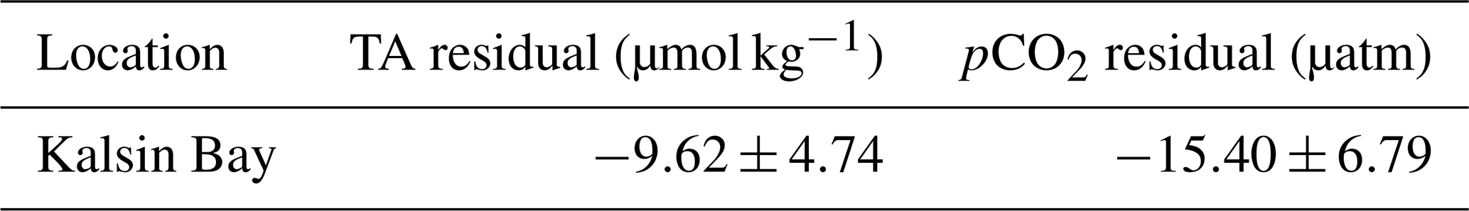
We calculated a site-specific salinity-TA relationship for Kalsin Bay, as the Evans et al. (2015) relationship massively underestimated the resulting pCO₂ values (Table A1). Using 6 of the 9 discrete bottle samples, a linear model was created:

$$\begin{array}{}\text{(A1)}& \text{Total alkalinity}=\mathrm{Salinity}\cdot \left(-\mathrm{5.613}\right)+\mathrm{2306.137},\end{array}$$

The last 3 discrete samples were treated the same as above, and the final residual for pCO₂ demonstrated a much better match than the Evans et al. (2015) relationship (Table A3).

Table A3 The residuals associated with the difference between the measured total alkalinity and resulting estimated pCO₂ value and a total alkalinity value predicted by Eq. (A1) and its resulting estimated pCO₂ value. Values are shown as the mean ± standard deviation.