Determination of the height of deep-sea mooring lines above seafloor using turbulence measurements

Height variations O(1) m of closely spaced moored oceanographic instrumentation are difficult to measure in the deep sea, requiring high-accuracy pressure sensors preferably on all instruments in a mooring-array. In this paper, an alternative method for relative height determination is presented using 2 m spaced high-resolution temperature sensors moored on multiple 9.5 m-spaced lines in the deep Western Mediterranean Sea. While it was anticipated that height variations between lines could be detected under near-homogeneous conditions via adiabatic lapse rate O(10⁻⁴ °C m⁻¹) by the 3 × 10⁻⁵ °C-noise-level sensors, such was prevented by the impossibility of properly correcting for short-term bias due to electronic drift. Instead, a satisfactory height determination was achieved during a period of relatively strong stratification and large turbulence activity. By band-pass filtering data of the highest-resolved turbulent motions across the strongest temperature gradient, significant height variations were detectable to within ±0.2 m.

1 Introduction

Height variations in moored oceanographic instrumentation can occur above unknown topographic features such as small rocks and gullies and due to line stretching by buoyancy force. For example, 0.005 m diameter steel cables (breaking strength ∼ 20 kN, where kN is Kilo Newton) stretch about 0.1 % of cable length under 1.25 kN tension, and 0.3 % under 4 kN tension for common oceanographic (e.g., https://www.spaceagecontrol.com/calcstre.htm, last access: 6 May 2026). If closely-spaced mooring lines and attached instrumentation are used, one may need to correct for the unknown height variations, for example to be able to distinguish thin O(1) m stratified layers. Such a correction is possible using high-resolution temperature sensors.

In this technical-performance paper, deep-sea instrumental-height determinations will be demonstrated using 45 mooring lines of 125 m tall and 9.5 m apart horizontally each holding 65 self-contained high-resolution temperature “T”-sensors in a 70 m diameter steel-pipe ring (van Haren et al., 2021). Each line, nylon-coated 0.005 m diameter steel cable, was pulled up by a net buoyancy of 1.25 kN, imposed by a single buoy on top, and was attached to the anchoring ring via a suspended steel-cable grid. The problem of this set-up was not so much the vertical-line stretch, but the unknown suspension of the steel-cable grid. In contrast with a fixed-anchor on a single-line mooring, the steel-cable grid has different heights between the anchoring steel pipes.

The ring was moored on a flat seafloor in nearly 2500 m deep weakly density-stratified waters of the Western Mediterranean Sea. The “large-ring mooring” was constructed for three-dimensional studies of deep-sea internal waves, their breaking and turbulence generation, to learn more about their dynamical development via short movies (van Haren et al., 2026) and detailed statistics.

2 Materials and Methods

A nearly half-cubic-hectometer of seawater was sampled using 2925 self-contained updated high-resolution, stand-alone T-sensors, new version “NIOZ4n”. The ensemble large-ring mooring (Fig. 1a) was deployed in drag-parachute controlled free-fall at the < 1° flat and 2458 m deep seafloor of 42°49.50^′ N, 006°11.78^′ E of the Western Mediterranean Sea in October 2020 (Fig. 1b). The mooring was near the site of neutrino telescope KM3NeT/ORCA (Adrián-Martinez et al., 2016) off the coast of Toulon, France, just 10 km south of the steep continental slope (and 5 km from its foot in the abyssal plain).

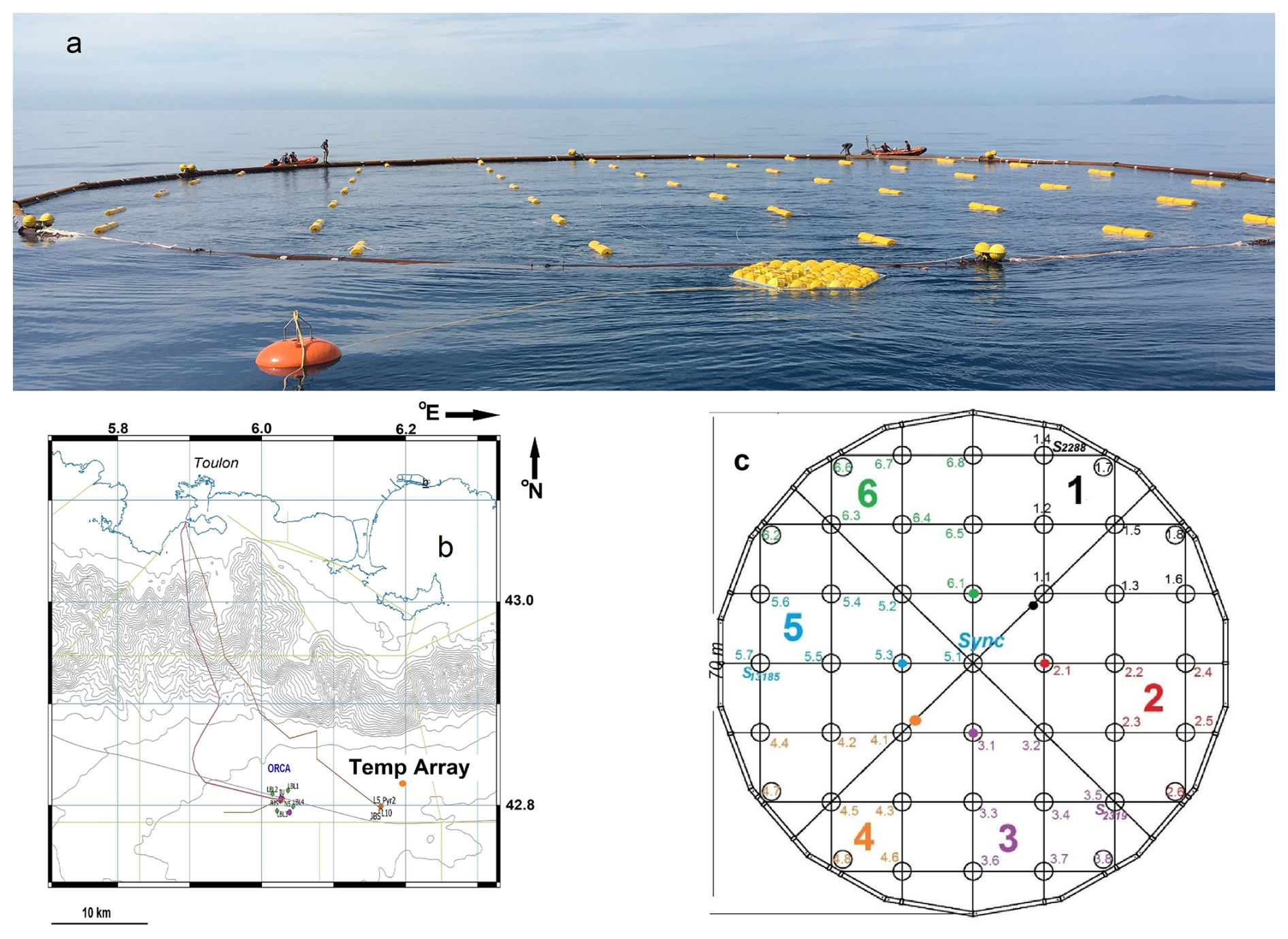
Figure 1 Large ring in fold-up form at sea, during deployment just prior to finish the opening of air-valves. The front part of the large steel-pipe ring is already underwater. Almost all top-buoys of the 45 small-ring-compacted mooring lines are visible. In the front still outside the ring, the yellow drag parachute and orange pick-up buoy are floating. (b) Location named “Temp Array” (orange dot) off southern France. The mooring is well east of main neutrino telescope “NT” site “ORCA” of KM3NeT (Adrián-Martinez et al., 2016) and just northeast of the former ANTARES NT-site. Isobaths are given every 100 m. (c) Layout of the large-ring mooring viewed from above, with steel-cable grid and small-rings numbered in six synchronisation groups. Lines 14, 35 and 57 (omitting the decimal point) held a current meter at the top-buoy. Corner-lies are, in clockwise direction: 17, 18, 26, 38, 48, 47, 62 and 66.

Figure 1c shows the numbering of 45 vertical mooring lines, which were ordered in six groups for synchronisation purposes. As with all NIOZ4 T-sensors (van Haren, 2018), the individual clocks were synchronised via induction to a single standard clock on the mooring-array every 4 h, so that all T-sensors were sampled within 0.01 s. Three buoys also held a Nortek AquaDopp single-point acoustic current meter. Details of design, construction and deployment are given in van Haren et al. (2021).

With the help from Irish Marine Institute Remotely Operated underwater Vehicle (ROV) “Holland I” on board Dutch R/V Pelagia, all lines with T-sensors were successfully cut and recovered in March 2024. Of the 45 lines, 43 were in good mechanical order, line 1.8 (line 8 of synchronization group 1; henceforth indicated without decimal point) was hit by the drag parachute whereby 10 sensors were lost, and line 65 was about 0.5 m lower than nominal because of a loop in the vertical line near the cable grid. Only line 36 did not register synchronisation, possibly due to an electric wire failure. Three T-sensors leaked and < 10 were shifted in position due to tape malfunctioning. In total 2902 out of 2925 T-sensors functioned as expected mechanically.

Due to unknown causes all T-sensors switched off unintentionally when their file-size on the 8 GB Kingston memory card reached 30 MB. It implied that a maximum of 20 months of data was obtained, which were recorded at an interval of once per 2 s. After post-processing, 50–150, depending on moment in the record and type of analysis, extra T-sensors are not further considered due to electronics, noise problems. With respect to previous NIOZ4 version, here named “NIOZ4o”, the slightly modified electronics resulted in about twice lower noise levels of $\mathrm{3}\times {\mathrm{10}}^{-\mathrm{5}}$ °C and twice longer battery life.

Laboratory-bath calibration yielded a relative precision of < 10⁻³ °C (van Haren, 2018). Instrumental electronic drift of typically 10⁻³ °C per month after aging was primarily corrected by referencing daily-averaged vertical profiles, which must be stable from turbulent-overturning perspective in a stratified environment, to a smooth, commonly third-order, polynomial without instabilities (van Haren and Gostiaux, 2012). Because vertical gradients of temperature, and thus density, are so small in the deep Mediterranean so that buoyancy frequency N=O(f), where f denotes the inertial frequency, a secondary drift correction was applied. For this correction, reference was made to periods of typically one-hour duration that were quasi-homogeneous with temperature variations smaller than instrumental noise level (van Haren, 2022). Such > 125 m tall quasi-homogeneous periods existed on days 350, in 2020, 453 and 657, both −366 in 2021, in the records. These two drift corrections allowed for proper calculations of turbulence values using the method of Thorpe (1977), as extensively described for moored T-sensors in van Haren and Gostiaux (2012) and van Haren (2018), under weakly stratified conditions. As will be demonstrated in Appendix A, under very weakly stratified conditions with N< 0.5f a tertiary drift correction involved low-pass filtering of data. This additional correction addresses short-term drift that was about 2–3 times larger in NIOZn than in NIOZo T-sensors.

3 Results

While a single-line mooring attached to an anchor at the seafloor may modify the nominal positions of instrumentation due to buoyancy-stretch of typically 0.1 %–1 % of the total line length, depending on amount of buoyancy and line fabric and make, the large-ring mooring will experience an additional differential positioning due to the variable anchor height of the cable grid. Given the anchor being the steel ring, the distributed buoys on top of each of the 45 lines are expected to pull the steel-cable grid (Fig. 1) up in the form of a dome. Hence, different heights are expected for different lines above the, presumed flat, seafloor. Simple geometrical models mimicking a dome will be compared with observations of height variations between the different mooring lines.

Prior to deployment, stretch-tests were performed with the grid's steel cable on a harbour quay. Under nominal tension of the planned buoyancy it was found that the exerted tension delivered a measured cable stretch to a value that the typical angle of grid inflection was expected to amount 5°. This angle to the horizontal could not be verified from visual inspection using ROV, although at various images a non-zero angle is discernible, which also seems to vary between different cable sections in the grid (Fig. 2a), as, e.g., in a dome.

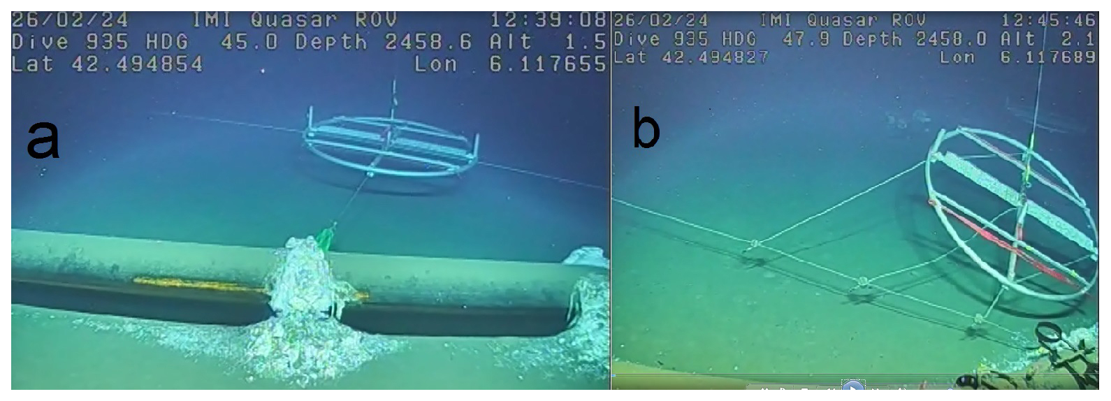
Figure 2 Underwater video stills of small-rings demonstrating steel-cable grid elevation and cable-inclinations. The 0.61 m diameter steel pipe in the foreground is part of the large anchoring ring, which sank 0.07 ± 0.02 m in the sediment of the < 1° flat seafloor. All steel cables are attached to the middle of the steel pipes, and thus at height h=0.24 m above sediment. (a) Line 44 (cf. Fig. 1c). To the right of the small-ring the wire visibly makes a larger angle to the horizontal than to the left. (b) Estimating height of “corner-line” 47, see text. (Images from video by ROV Holland I).

Eight “corner-lines” (Figs. 1c, 2b) were also displaced to an amount not precisely verifiable from ROV-inspection. These lines were attached differently to the steel-cable grid as they could not be attached directly to their intersection points at the steel ring. Estimating the height of corner-line can be attempted from Fig. 2b. Visually, the right side of the small ring holding a vertical line in its center does not touch seafloor and the small ring rotates around the smallest of three short assist cables of which the centre is elevated to approximately h=0.6 m above seafloor. If angles are measured on the basis of vertical/horizontal ratio $\mathrm{4}/\mathrm{4.5}$, then the small-ring makes an angle of about 40° to the horizontal, so that its center is 0.8 m above the edge of the small-ring. In that case, the corner-line will start at h=1.0 m.

3.1 Parabola model

Taking the 5°-angle due to distributed tension stretch as starting point, some simple models of half cable-grid cross-section can be made (Fig. 3). Quasi-parabola and straight-cable models are considered. Considering that grid attachments are made in the center of the large-ring pipes at 0.3 m, the models start from that height above seafloor. All grid attachments were made to extra enforced steel rings that were bolted around the pipes, to guarantee the pipes remain circular. The steel rings and pipes were protected against corrosion with zinc anodes (Fig. 2).

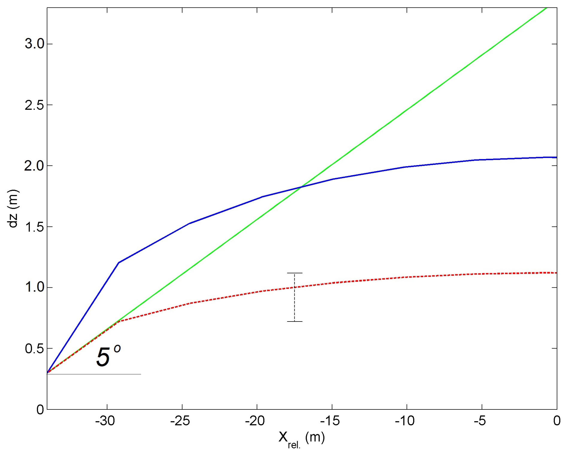
Figure 3 Some expected quasi-parabola and straight-line models, for half centre steel cable of large-ring mooring grid. The seafloor is at the horizontal axis, the cable-grid attachment to the large-ring is for a steel pipe at a solid floor. The green straight line has a fixed angle of 5° with the horizontal, which angle was established after in-port tension tests. The blue (solid line, 5 m discretized) parabola model intersects the green line halfway, so that its top is at h=2.07 m. If an overall maximum angle of 5° is maintained (red dashed model), the parabola top is at h=1.12 m, and the first vertical line attached to relative horizontal position $x_{\mathrm{rel}}=-\mathrm{29}$ m will be at h=0.72 m.

The simplest, albeit unrealistic, straight-cable model makes a fixed angle of 5° (green model in Fig. 3). A slightly better model is a paraboloid, a 3D form of the mathematical parabola, as would be approximately found in a weighed cable grid held upside down under gravity. A 5 m discretized parabola model intersecting the straight-cable model halfway will have its top at h=2.07 m above (blue model). The steepest part, exceeding 5°, of the cable in this model has a horizontal distance of 5 m to the large ring, which corresponds with the position of, e.g., line 57 (cf. Fig. 1c). In the model, line 57 has its lowest T-sensor at h=1.2 m. If an overall maximum angle of 5° is maintained, the top of that parabola model will be at h=1.12 m, and the first line inside the large ring will have its lowest T-sensor at h=0.72 m (red model). In an attempt to verify these cable-grid models, data from the altimeter and, in a relative sense, the pressure gauge of the ROV were used. They gave a value of $h=\mathrm{0.7}\pm \mathrm{0.1}$ m after the ROV had landed on the small-ring of the first line of the grid's centre cable.

If the maximum-5° parabola model is correct, all vertical lines are a maximum of 0.4 m, or ±0.2 m, apart vertically. This is difficult to correct for in practice. Unfortunately no pressure sensors were available on the vertical lines, the three mounted on current meters being too inaccurate, to quantify height variations between lines. As a result, quantification is sought using the T-sensor data to verify, and possibly improve when necessary, above geometrical model values.

3.2 Adiabatic lapse rate height-determination method

Considering that the T-sensors have a noise level of 10⁻⁵ °C, potential temperature differences of > 5 × 10⁻⁵ °C are statistically significantly detectable, in theory. Thus, given local deep Western Mediterranean adiabatic lapse rate of $\mathrm{\Gamma }=-\mathrm{1.7}$ × 10⁻⁴ °C m⁻¹ (here for simplicity a pressure of 10⁴ Pa is transferred to a vertical distance of 1 m), vertical height differences of > 0.3 m are potentially detectable using T-sensor data under near-homogeneous conditions in which temperature variations are predominantly due to compressibility effects. Such conditions do occur in the deep Western Mediterranean regularly, see the lower 250 m above seafloor in a shipborne-CTD profile (Fig. 4). Γ dominates the temperature lapse with the vertical in Fig. 4a. In time series from moored T-sensor data, near-homogeneous conditions over 125 m vertical range occur about 60 % of the time (Fig. 5a). These conditions lead to very low temperature variance across all frequencies outside instrumental white noise (Appendix A).

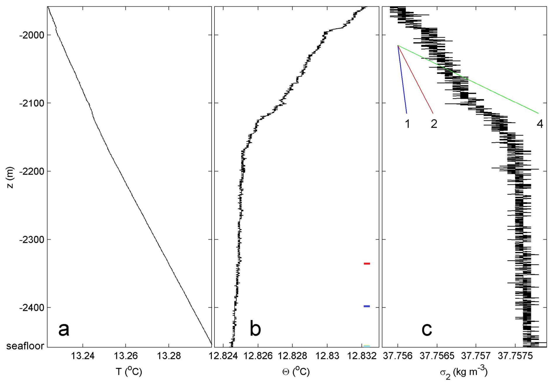
Figure 4 Lower 500 m of shipborne CTD-profile data obtained near the large ring during mooring deployment. (a) In situ temperature. (b) Conservative Temperature (IOC et al., 2010), data in (a) corrected for compression. Small colour bars indicate nominal heights of moored T-sensors at lowest (cyan), middle (blue) and upper (red) positions. (c) Density anomaly referenced to 2 × 10⁷ Pa. The sloping lines indicate several stratification rates in terms of buoyancy frequency N=xf, x=1, 2, 4 times the local inertial frequency f.

However, a complicating factor in “adiabatic lapse rate height-determination” method is the electronic drift of T-sensors, which varies in intensity per sensor but typically amounts about 10⁻³ °C per month. While the value is one order of magnitude larger than the adiabatic lapse rate per unit length, in principle T-sensors attached to a particular vertical line can be corrected to within a precision, i.e. relative accuracy, of 10⁻⁴ °C (van Haren, 2018). All depends on a calibration with a precision of < 5 × 10⁻⁴ °C, which is achievable using a thermostatic bath with constant temperature levels to within $\pm {\mathrm{10}}^{-\mathrm{4}}$ °C of their preset values. The standard post-processing correction is by fitting a smooth curve over sufficiently time-averaged vertical temperature profile that must be stable over an inertial period. When the temperature range is not too large, above precision is obtainable with some effort and careful search in the data. In the weakly stratified deep Mediterranean however, this correction is not achievable between different lines, because the low precision is not transferrable to a low absolute accuracy.

As a result, the height determinations from translated temperature differences between lines attached to the steel-cable grid are too large and erratically distributed (Fig. 6). Obviously, there is no consistency between lines in the image of Fig. 6, which shows no signs of expected lower relative values at the edges close to the ring and higher values near the center, following parabola models as in Fig. 3. Moreover, the variation in values is nearly an order of magnitude greater than expected from the parabola models in Fig. 3. Clustering per calibration – approximately 190 T-sensors are used in the thermostatic bath per cycle (van Haren, 2018) – does not give improvement of consistency in the image (not shown).

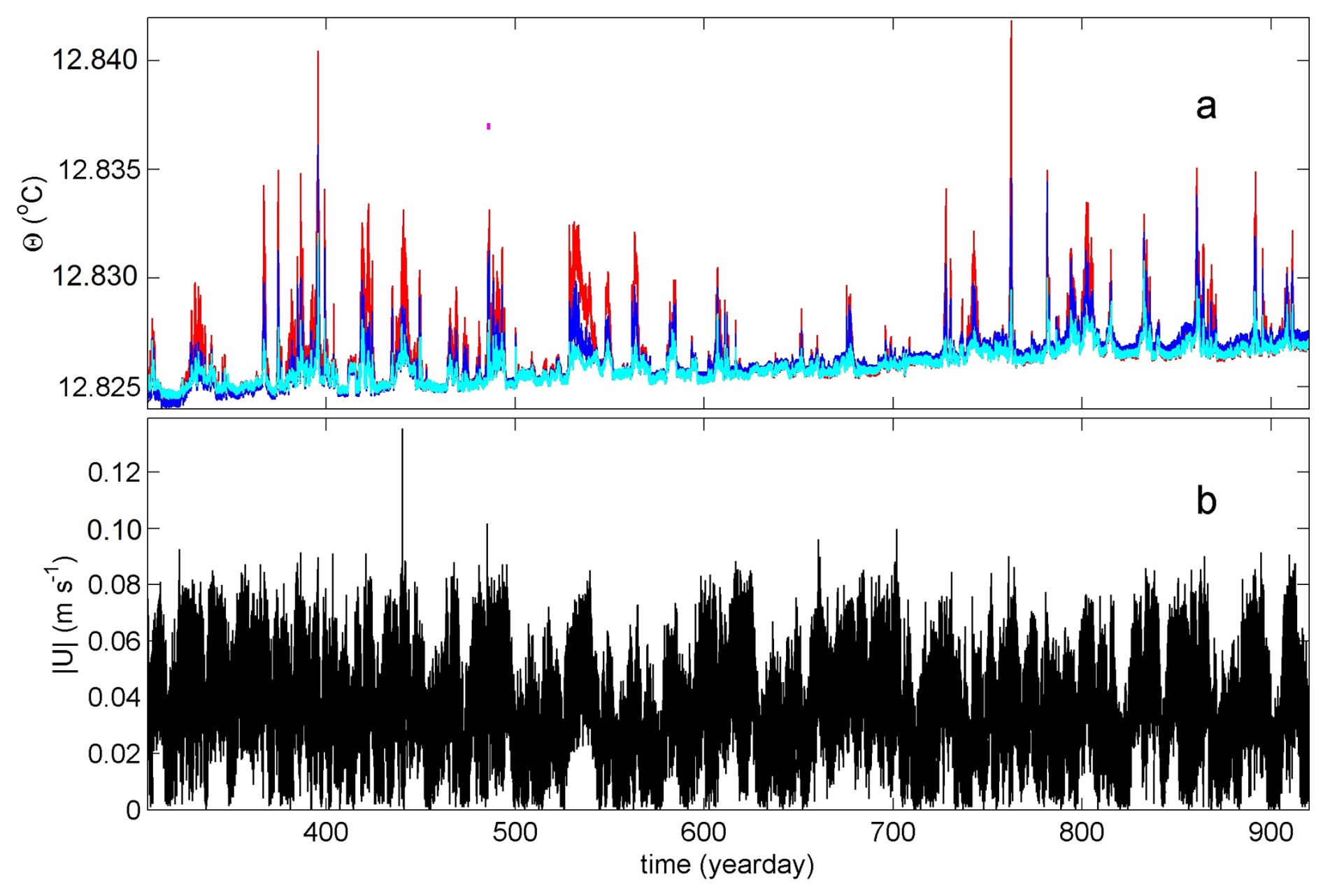
Figure 5 Overall 20-month time series of moored temperature and current meter data. (a) Conservative Temperature at h=1 (cyan), 63 (blue) and 125 m (red) cf. Fig. 4b of arbitrary line 53. Data are subsampled at once per 6 s and not corrected for electronic-drift bias. The magenta dot indicates day 485. (b) Unfiltered current speed at h=126 m of line 14.

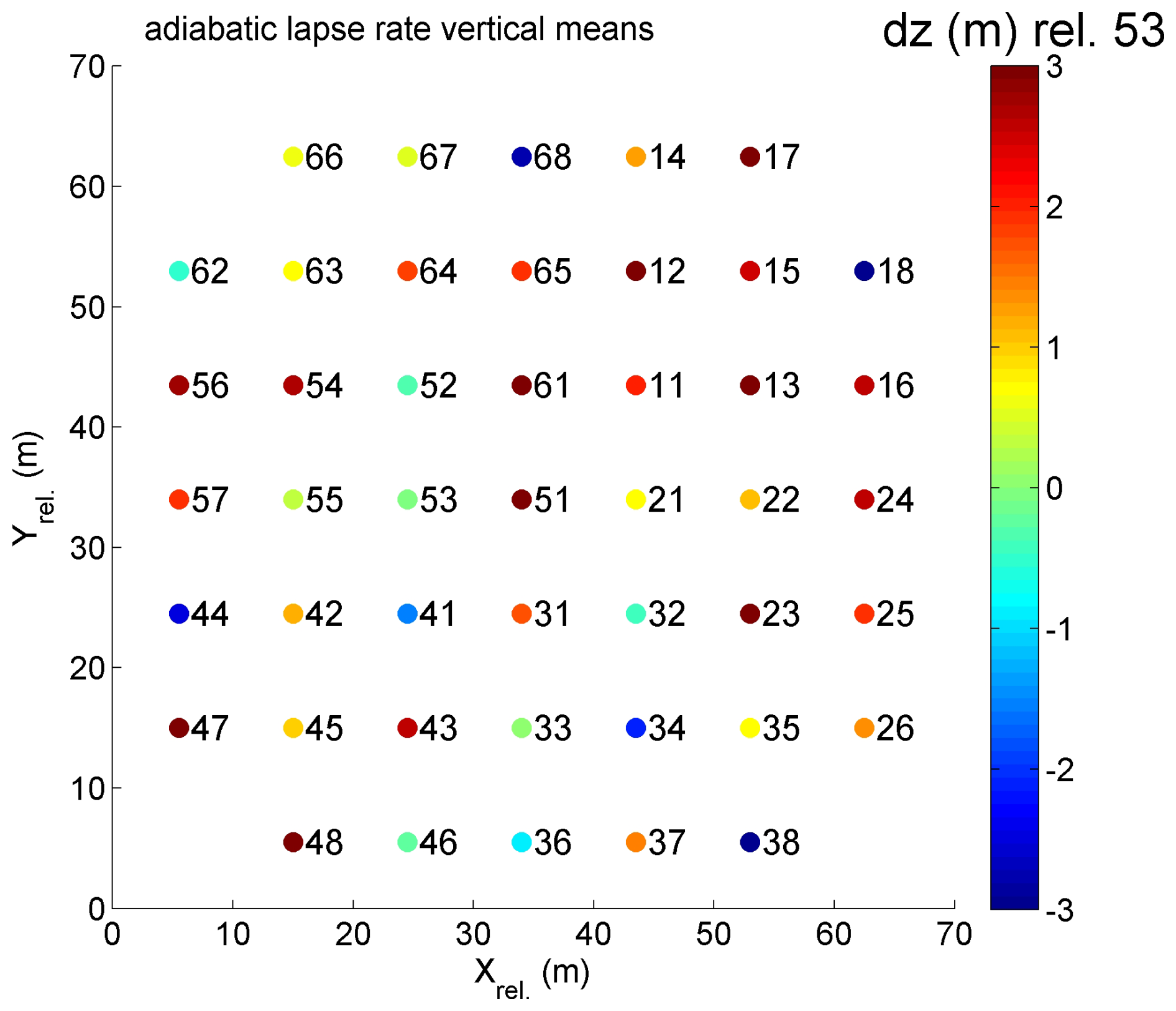
Figure 6 Vertical displacement calculation for vertical lines of the large-ring mooring using the local adiabatic lapse rate Γ. This height-determination method is based on temperature shift per line after calibration and drift correction for near-homogeneous period 350.04–350.08, with arbitrary line 53 as reference. The conversion of meters into degrees Celsius is via $\mathrm{\Gamma }=-\mathrm{1.7}\times {\mathrm{10}}^{-\mathrm{4}}$ °C m⁻¹, so that a vertical difference of dz=3 m reflects approximately $\mathrm{5}\times {\mathrm{10}}^{-\mathrm{4}}$ °C.

3.3 Turbulence variance height-determination method

As the adiabatic pressure effect on temperature is not a suitable measuring method for the expected doming of the steel-cable grid inside the large ring, another method is sought. In contrast with the adiabatic lapse rate method, this other method is not working under near-homogeneous conditions. Instead, it works when vertical temperature stratification is rather large, with peaks resulting in N=6f, and turbulent temperature variations are large (Figs. 5a, 7, 8). The combination of these two conditions, relatively large stratification and large turbulence, seems counter-intuitive, as stratification is generally considered to suppress turbulence. Whilst stratification indeed suppresses the vertical length-scale of turbulence, it may have variable effects on temperature variance.

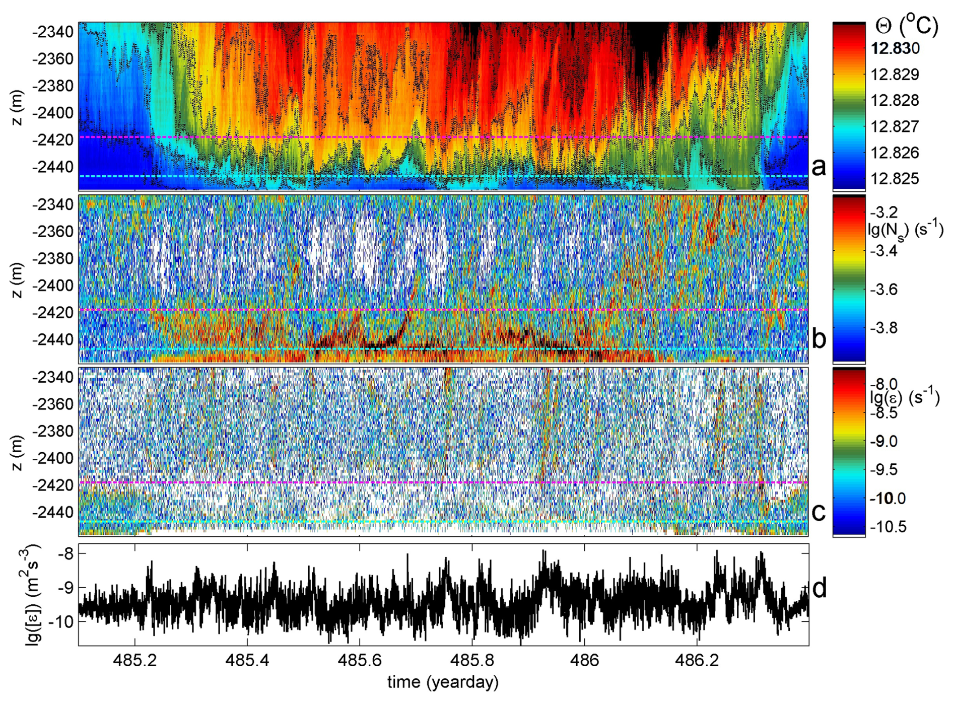
Figure 7 Thirty-one hours of data from line 53 during a turbulent passage of relatively warm water. Horizontal dashed magenta and cyan reference lines are at h=40 and 11 m above seafloor, respectively. (a) Time-depth plot of Conservative Temperature with black-dotted contours every 10⁻3 °C, low-pass filtered “lpf” with cut-off at 3000 cpd (cycles per day). (b) Logarithm of 2 m small-scale buoyancy frequency from reordered profiles of data in (a). (c) Logarithm of non-averaged displacement values from data in (a). following the reordering method by Thorpe (1977) and cast in units of turbulence dissipation rate. (d) Time series of logarithm of turbulence dissipation rate averaged over the 124 m vertical extent of T-sensors.

In case of the deep Western Mediterranean, relatively large vertical temperature gradients of a few 10⁻³ °C over O(10–100) m occur with the advection of warmer waters (Figs. 5a, 7a). The advection is regularly slanted towards the vertical, either induced by internal-wave action and/or by sub-mesoscale and mesoscale eddies, as inferred from quasi-3D movies (van Haren et al., 2026). When mainly governed by planetary vorticity deflection, it represents in part convection-turbulence that appears in a vertically stratified environment at mid-latitudes (Marshall and Schott, 1999). All warming events observed thus far associate with considerable turbulence. In the entire time series (Fig. 5a) no significant cooling events occur. Current speeds (Fig. 5b) seldom exceed 0.1 m s⁻¹ and thus there is no evidence strong flow events such as associated with deep dense-water formation that might occur in late winter.

Due to the relatively low-noise T-sensors, deep Western-Mediterranean waters can be characterized by frequency (ω) spectra in which turbulence manifests itself over a range of at least two orders of magnitude (Fig. 8), approximately across 10 < ω < 3000 cpd (cycles per day), under the relatively large turbulence conditions. Outside this band, spectra are dominated by internal waves, for ω < 10 cpd, and roll-off to instrumental white noise, for ω > 3000 cpd. A strong temperature gradient produces high-frequency internal waves, but is also accompanied by turbulent eddies, probably as a result of breaking internal waves. Under near-homogeneous conditions similar temperature spectra are found, except that the variance is two orders of magnitude lower and turbulence drops into instrumental noise at about 500 pd (cf. Fig. A2).

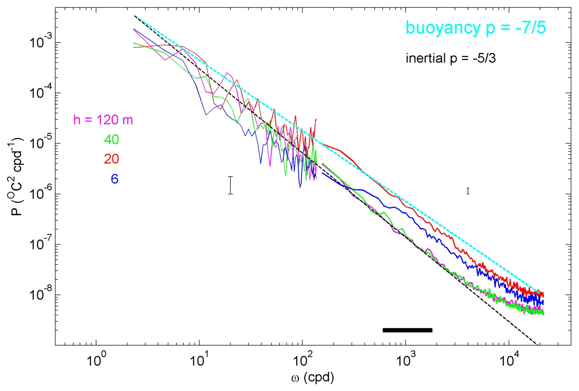
Figure 8 Unscaled frequency spectra, patched from weakly and heavily smoothed parts, for four T-sensors of line 53 at indicated heights h above seafloor, averaged over the 1.3 d period of Fig. 7 for unfiltered data. Spectral slopes ω^p for inertial and buoyancy subranges of turbulence are indicated with straight dashed lines and exponents p. The horizontal black bar indicates frequency range of the pass-filter band that is applied for the turbulence-variance method of height determination.

Here, we take the high-frequency portion $\mathrm{\Theta }\prime (t,z)$ of the well-resolved turbulence band and, somewhat arbitrarily, band-pass filter between 600 < ω < 1800 cpd (frequency range indicated by the black bar in Fig. 8) that is certainly outside internal wave and white noise bands. Although temperature variations in this range are part of inertial subrange of isotropic turbulence (Kolmogorov, 1941) reflecting a continual transfer between large energy-containing turbulence scales and small dissipative scales via shear-induced motions, such are mainly found well away from the seafloor. Within h= O(10) m from the seafloor, motions are partly of isotropic nature and partly of anisotropic convection-turbulence nature in a buoyancy subrange (Bolgiano, 1959; Obukhov, 1959), which manifests at all heights in the range 10 < ω < 100 cpd, albeit the spectral smoothing is coarse. Irrespective of a variation in slope and turbulence behaviour, the main goal here is the practical use of temperature (turbulence) variance outlined below. Future investigations will be directed to improve statistics in part by averaging data from the 45 lines and data from different periods of stratified turbulence.

During such a period of slanted warm waters from above, temperature variance may be relatively low within a few meters from the seafloor, but it increases to high levels well above common interior-values in O(10) m above seafloor (Figs. 8, 9). The 1.3 d root-mean-square value of the 600–1800 cpd band-pass filtered signals is calculated for every T-sensor. In this example, the peak in turbulence-temperature variance is found around h=11 m. Above and below the peak one can take advantage of two depth-levels of high gradients in turbulence temperature-variance. Common interior-values are reached at about h> 40 m = h_sst, which could reflect the upper limit of layer of strong stratified turbulence (Figs. 7–9).

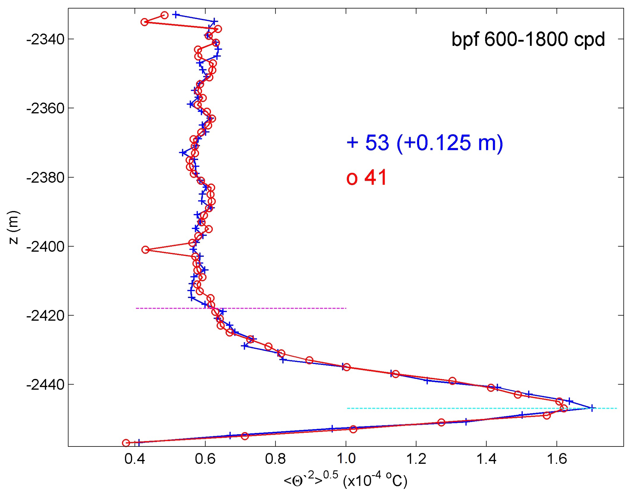
Figure 9 Vertical profiles of standard deviation of band-pass filtered “bpf” high-frequency turbulence signals for temperature data in Figs. 7a, 8 for two neighbouring lines, with off-set relative height determination. The variance-peak height (cyan-dashed line) corresponds also to the height of strongest layering in stratification in Fig. 7b. The magenta-dashed line delineates the vertical extent of enhanced temperature variance above interior values.

After referencing local turbulence temperature variance Θ′²(line, z) to the value of an arbitrary line(x), by subtracting Θ′²(line(x), z), taking the mean of two levels z1 and z2 and scaling with the 45-line average $<.>$ value of their vertical gradient $\langle \mathrm{d}\left(\mathrm{\Theta }{\prime }^{\mathrm{2}}\right)/\mathrm{d}z\rangle$ over dz = z2−z1, commonly the, here constant, 2 m distance between T-sensors, a transfer from temperature to height value is established. Hereby it is assumed that over the 1.3 d period the statistics are homogeneous over the mooring array. Heterogeneity is not expected to affect the average value over a period longer than the inertial period. Subsequently, below or above the peak value in Fig. 9, a height pattern can be computed relative to values of an arbitrary vertical line, 44 in this case (Fig. 10). Here, the pattern is given for height determination by computing across the largest gradient of temperature-variance, between T-sensors at h=3.5 and 5.5 m. An example of an eight times shorter period is given in Appendix B.

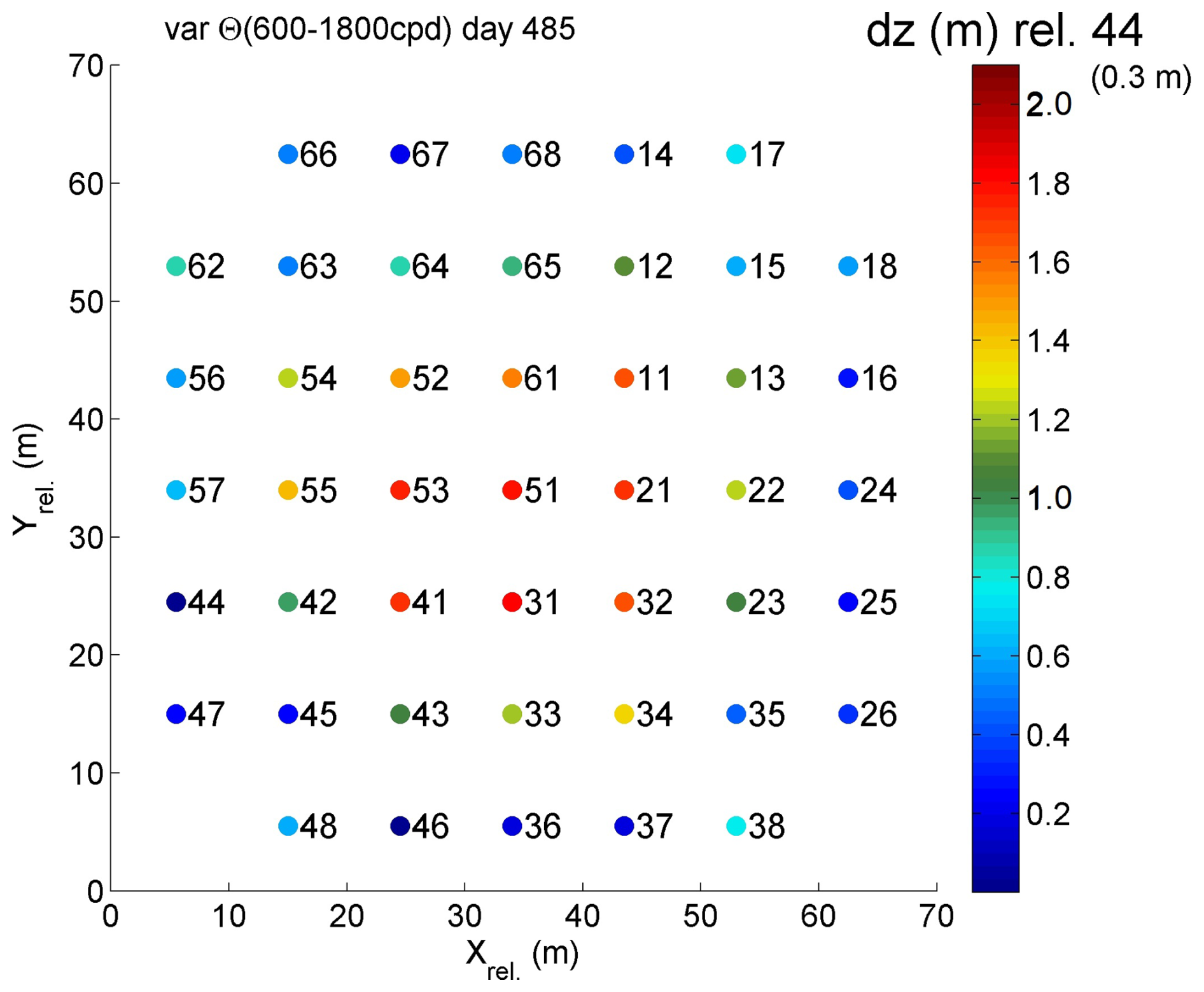
Figure 10 As Fig. 6, but for turbulence-variance height-determination method determined from profiles like in Fig. 9 using T-sensor data between positions 2 and 3 above seafloor, where the gradient in temperature variance is maximum, divided by the average gradient over 2 m. Values are given relative to those of line 44 (0.3 m), arbitrary line near the edge of the cable-grid.

The difference between this pattern and that in Fig. 6 is obvious. First, all values are between 0 and 2 m in Fig. 10, and a consistent statistical significance is found to within ±0.2 m. Cross-sections of the cable grid also confirm the doming of the pattern (Fig. 11). While the observed doming is close to the parabola models of Fig. 3, larger height-determination values than in the models are observed in the center, with slightly steeper overall grid cables that still roughly obey the maximum 5° slopes (Fig. 11). The ±0.2 m error range is easily verifiable after comparison with the provided bar. Corrections to vertical positioning of T-sensors are therefore feasible and necessary, because the difference between the center and edges of the cable grid is approximately 1.5 m.

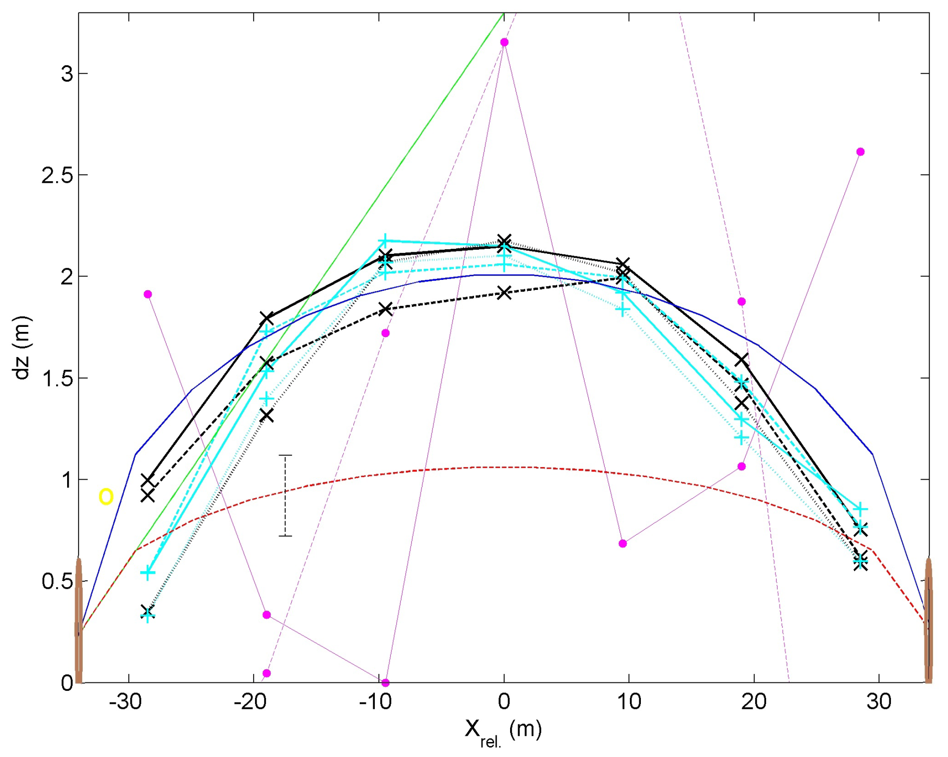
Figure 11 Constant-Y (black x graphs) and constant-X (cyan +) cross-sections without corner-lines of height determinations from Fig. 10 vertically shifted +0.3 m. Solid lines indicate center lines in both directions. Corner-line height determination is indicated by yellow o. For comparison, data in Fig. 6 are given for central lines with magenta dots (thin solid x-direction; dashed y-direction). In the background, models are given in green, blue and red of double distance than in Fig. 3.

3.4 Stratified turbulence quantification

The temperature variations of the well-stratified day 485 demonstrating the necessary height determination for the doming of the steel-cable grid show a background value of turbulence dissipation rate O(10⁻¹⁰) m² s⁻³. Reduced values O(10⁻¹¹) m² s⁻³ are basically only found within a few meters from the seafloor, underneath the largest 2 m small-scale stratification with maximum buoyancy-frequency values of $N_{max}\approx \mathrm{1.6}$ × 10⁻³ s⁻¹ (Fig. 7). This is observable in time-depth plots of temperature, small-scale stratification and non-averaged turbulence dissipation rate “values”. The largest overturns, which dominate the vertically averaged values of turbulence dissipation rate, have a scale O(100) m (Fig. 7a, c). Turbulent overturns reach close to the seafloor, but only sporadically touch it, mostly at begin and end of the warm-water depression. Coarsely every two hours, 124 m vertically averaged turbulence dissipation rate peaks in value (Fig. 2d). The h=40 m of elevated high-frequency temperature variance (Fig. 9) and stratification (Fig. 7b) show non-negligible turbulence dissipation rate values with further elevated values reaching the seafloor before and after the warm-water passage (Fig. 7c).

Time-depth mean values from the 1.3 day period are for turbulence dissipation rate [〈ε〉] = $\mathrm{6}\pm \mathrm{3}\times$ 10⁻¹⁰ m² s⁻³ and for turbulent diffusivity [〈K_z〉] = 1.4 ± 0.7 × 10⁻³ m² s⁻¹ under [〈N〉] = 2.8 ± 0.3 × 10⁻⁴ s${}^{-\mathrm{1}}\approx \mathrm{3}f$. These 1.3 d, 124 m mean turbulence values are about one order of magnitude larger than open-ocean values observed in stratified waters well away from boundaries (Gregg, 1989; de Lavergne et al., 2020; Yasuda et al., 2021). The reader is reminded that the experiment was located close to the foot of the continental slope, where the strong Liguro-Provençal current flows, (internal) tides are weak, and total, (sub-)mesoscale plus near-inertial, water-flow speeds never exceed 0.1 m s⁻¹.

Although the warm-water event of Fig. 7 is of relatively strong turbulence, it is not exceptional and elevated temperature-stratification and -variance alternate in time with near-homogeneous episodes throughout the 20-month records (Fig. 5a). This will be reported elsewhere in more detail, notably using three-dimensional investigations.

4 Conclusions

The expected height variation due to vertical buoyancy pull across a steel-cable grid, which was suspended within a large anchoring steel-pipe ring, was modelled as an inverted parabolic with maximum 5° angle to the horizontal. To verify the height variation of the instrumented vertical mooring lines across the grid, we expected to use an observational period with negligibly small vertical density, abd thus temperature, stratification so that the adiabatic lapse rate $\mathrm{\Gamma }=\mathrm{d}T/\mathrm{d}z$ would dominate vertical temperature variations T(z). The T-sensors have a noise level of about 3 × 10⁻⁵ °C, while $\left|\mathrm{\Gamma }\right|\approx \mathrm{1.7}$ × 10⁻⁴ °C m⁻¹ in the deep Western Mediterranean and thus is potentially measurable by sensors nominally 2 m apart vertically. However, the sensor's electronic drift at all scales turned out insufficiently correctable under near-homogeneous conditions.

Instead, a mooring-height determination was achieved during a period of relatively large stratification, during a slump down of warm water presumably slanted from above and induced by internal waves. By band-pass filtering the highest resolved turbulence variance, mainly from inertial subrange, across the strongest temperature gradient, the dome of pulled-up grid was significantly detectable, and fine-tuned a parabola model with height variations between the moorings of correctable (0.5–2.0) ± 0.2 m.

The impact of investigating turbulence signals from high-resolution moored T-sensors in the deep Mediterranean is several-fold. First, it demonstrates the dynamics of internal-wave breaking governed by either near-inertial or sub-mesoscale motions slumping relatively warm waters to within a few meters above the seafloor. Thereby, an episodic-average turbulence dissipation rate is provided, which is about ten times larger than ambient values above a flat seafloor. The enhanced turbulence affects deep-sea life. Deep-sea turbulence is studied more elaborately in a future report.

Second, the strong vertical variation in turbulence temperature-variance profiles, across relatively large local vertical temperature gradients, may be useful for height determinations in nearby moorings over flat seafloors also in shallow seas, and, more difficult, above sloping seafloors, whereby a correction may be applied for unknown mooring-line stretch under tensioning by buoyancy. Such height determinations may also be necessary when moorings are accidentally placed on small rocks or in small gullies. The resulting determination demonstrated that the parabola model based on in-house line-tensioning was adequate and required only secondary adjustment in the slightly steeper cables of the underwater large-ring mooring, albeit all showed < 5° sloping to the horizontal as anticipated from the in-house tests.

Appendix A: Extra drift correction for T-sensors in near-homogeneous waters

When waters are very weakly stratified or near-homogeneous with N< 0.5f over the range of moored T-sensors, a short-term drift error may emerge. This drift partially causes the impossibility to determine instrumental height variations under such conditions. Albeit electronic drift is well known to occur on long timescales of weeks-months, short-term hourly drift may appear because of nonlinear temperature dependency and/or inadequate contact between the Negative Temperature Coefficient NTC thermistors and the environment through the glass tube and its contact paste. NTC thermistors are the measuring component of NIOZ T-sensors. This short-term drift was previously observed in NIOZ4o deep-trench data and, especially clear, in air (van Haren and Bosveld, 2022). It turned out difficult to correct for. During a 2017/2018 test experiment in the deep Western Mediterranean it did not pose a great problem in NIOZ4o data. Unfortunately, NIOZ4n appear to have about twice larger short-term drift than previous NIOZ4o, despite their smaller long-term drift and smaller instrumental noise, both by a factor of two-three approximately. A correction for short-term drift of NIOZ4n is proposed below, with reference to NIOZ4o.

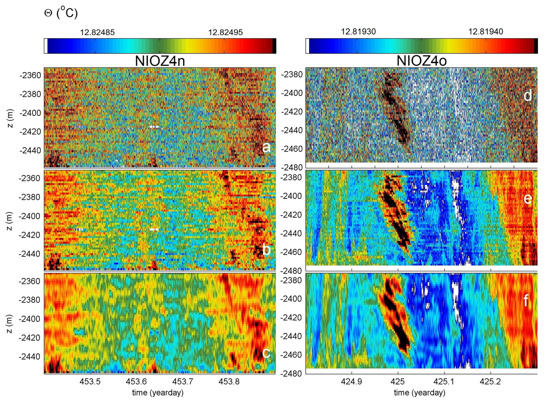
Figure A1 Half-day Conservative-Temperature data from h=1–104 m demonstrating the correction of short-term drift. The conditions are near homogeneous, as full the temperature range is only 1.7 × 10⁻⁴ °C during both the present experiment in 2020/2021 (left column) and during a test-experiment in 22 m deeper water in 2017/2018 (right column). (a, d) Unfiltered data, after post-processing involving calibration, referencing to CTD-, homogeneous-period-, and smooth-polynomial data. (b, e) Lpf with cut-off at 500 cpd. (c, f) Corrected for short-term drift: 500 cpd and 10 m vertical-scale lpf data.

Half-day NIOZ4n data (Fig. A1a–c) from arbitrary line 25 are compared with a 104 m tall set of NIOZ4o data (Fig. A1d–f). The investigated samples are from almost homogeneous waters, with a total colour-range over a Conservative-Temperature difference of only 1.7 × 10⁻⁴ °C, for both data sets. Although NIOZ4o are more noisy (Fig. A1a, d), the NIOZ4n show a more horizontal-stripy pattern that has different values through time, compared to T-sensors above and below. This is evidence of remaining bias due to short-term drift. Low-pass time filtering, with a cut-off frequency of 500 cpd, does not reduce these (Fig. A1b, e), but additional vertical filtering, with a cut-off wavenumber at 10 cpm, adequately removes the bias (Fig. A1c, f).

As a consequence of near-homogeneity, energetic overturning scales are expected to be large due to the reduced restoring force. In both data sets in the center of images, albeit clearer in the NIOZ4o, one notices a slanting jet of warmer waters over a vertical range of about 60 m in short bursts of 10–20 m. Such jets of convection turbulence were found abundant in the Mariana Trench (van Haren, 2023), but relatively rarely in the deep Mediterranean.

Depending on the rate of stratification, the vertical filter cut-off at 0.05–0.2 cpm (cycles per meter) is obtained after fine-tuning in an attempt to retain the relevant overturning scales as much as possible. Under weakly but stable stratified conditions 0.1–0.2 cpm is used, while under near-homogeneous and unstable conditions 0.05–0.1 cpm is used. The fine-tuning of the vertical filter concerns relatively adequate spectral improvement and turbulence calculations. Naturally, all data-corrections yield a certain loss of information, but it is informative to estimate how much the loss may be.

In 4-d-average spectra (Fig. A2) that include the 0.5 d period of Fig. A1, the impact of small-scale drift is seen to be larger for NIOZ4n (Fig. A2a) than for NIOZ4o (Fig. A2b). In these plots spectra are scaled with the slope of buoyancy subrange, for clarity. As a reference for the correction, the temperature difference ΔΘ (magenta spectrum) is taken between the two neighbouring T-sensors at h=29 and 31 m. That difference spectrum is compared with the spectrum of temperature data from the upper T-sensor (green). The magenta spectrum has a higher noise level by about a factor of two for ω> 100 cpd than that of the green spectrum. This is commensurate with random white noise.

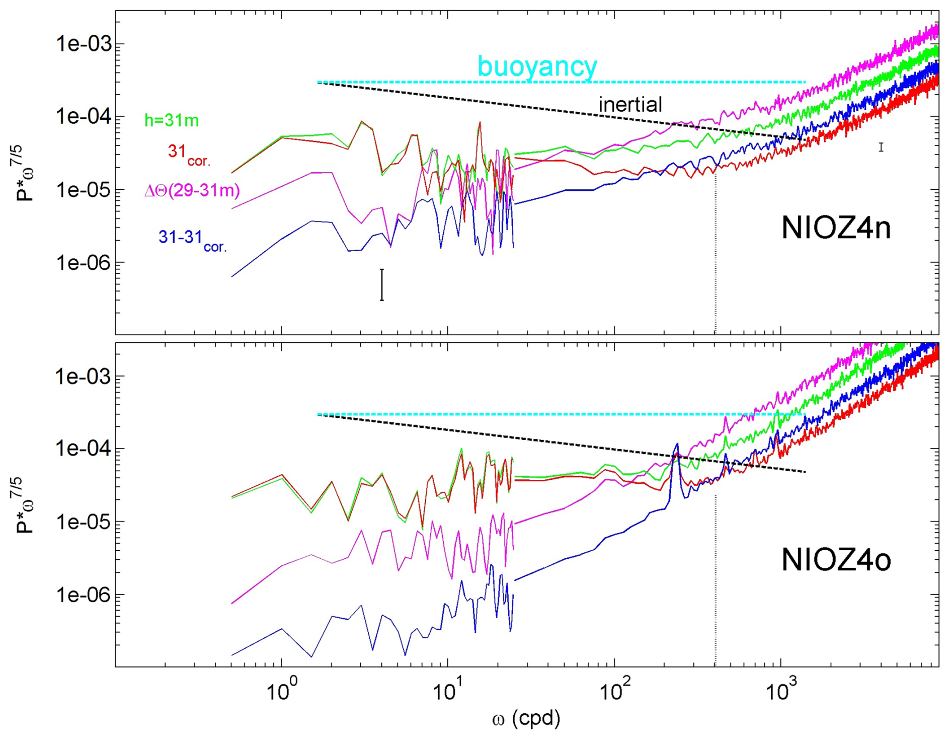
Figure A2 Four-day average spectra that are patched together from two, a weakly- and a heavily smoothed part, and scaled with the buoyancy-subrange slope (horizontal cyan). From 2 s sampled T-sensor data. The spectra demonstrate effects of and correction for short-term drift in T-sensor data around h=30 m during near-homogeneous periods between days 453–457, including those of Fig. A1. Plotted are spectra for unfiltered data (green), vertical temperature difference with data from T-sensor 2 m lower (magenta), 500 cpd and 10 m vertical scale corrected data (red), and the difference between green and red spectra (blue). For reference, the relative log-log plot slope is given for inertial subrange (black). The vertical dotted line at 400 cpd is explained in the text. (a) NIOZ4n data. (b) NIOZ4o data.

At lower frequencies, the magenta spectrum crosses the green spectrum around 50 and 150 cpd for Fig. A2a and b, respectively. This means that data are no longer dominated by white noise, but by other parametrizations, which are governed either by natural processes or by instrumental flaws other than noise. Around the crossing frequency, temperature spectra become horizontal following buoyancy-subrange scaling. This scaling, which represents convection turbulence of an active scalar (Bolgiano, 1959; Obukhov, 1959), was no longer dominant at frequencies higher than that of the crossing, more so in Fig. A2b than in Fig. A2a.

After correction by applying vertical low-pass-filtering (red), the weak slope towards lower frequencies, especially that of Fig. A2a, is correctly removed and white noise levels are lower. The spectral slope change to white noise is now at the same frequency, 400 cpd, for both data sets. The quasi-transfer function of correction depicted in the blue spectra is less steeply sloping for ω< 1000 cpd in Fig. A2a than in Fig. A2b, which demonstrates the larger effects of short-term drift correction for the NIOZ4n compared to the NIOZ4o. However, in both data sets of very weakly stratified deep-sea waters it prevents resolution of the transition from buoyancy and/or inertial subranges to the viscous turbulence dissipation range.

Resuming, after vertical-filtering correction, temperature data at ω< 400 cpd seem useful for turbulence calculations under weakly stratified conditions. Note that this correction is not needed during periods with relatively large temperature variance and stratified, generally more shear-induced, turbulence. For turbulence dissipation rate calculations, 10 %–30 % reduction is obtained from short-term drift correction. This reduction is well within the error range of a factor of two normally achieved for ocean turbulence data.

Appendix B: Height determination from a short warm-water period

Naturally the method sketched in Sect. 3.3 does not work under all circumstances. One requires a rather vigorous appearance of stratified warm-water turbulence to preferably reach close to the seafloor. Such periods are sought manually. Even a short 3.6 h period returns a reasonable estimate of the cable grid height (Fig. B1). It mimics Fig. 10, and has some larger noise level with values that remain within the error bar.

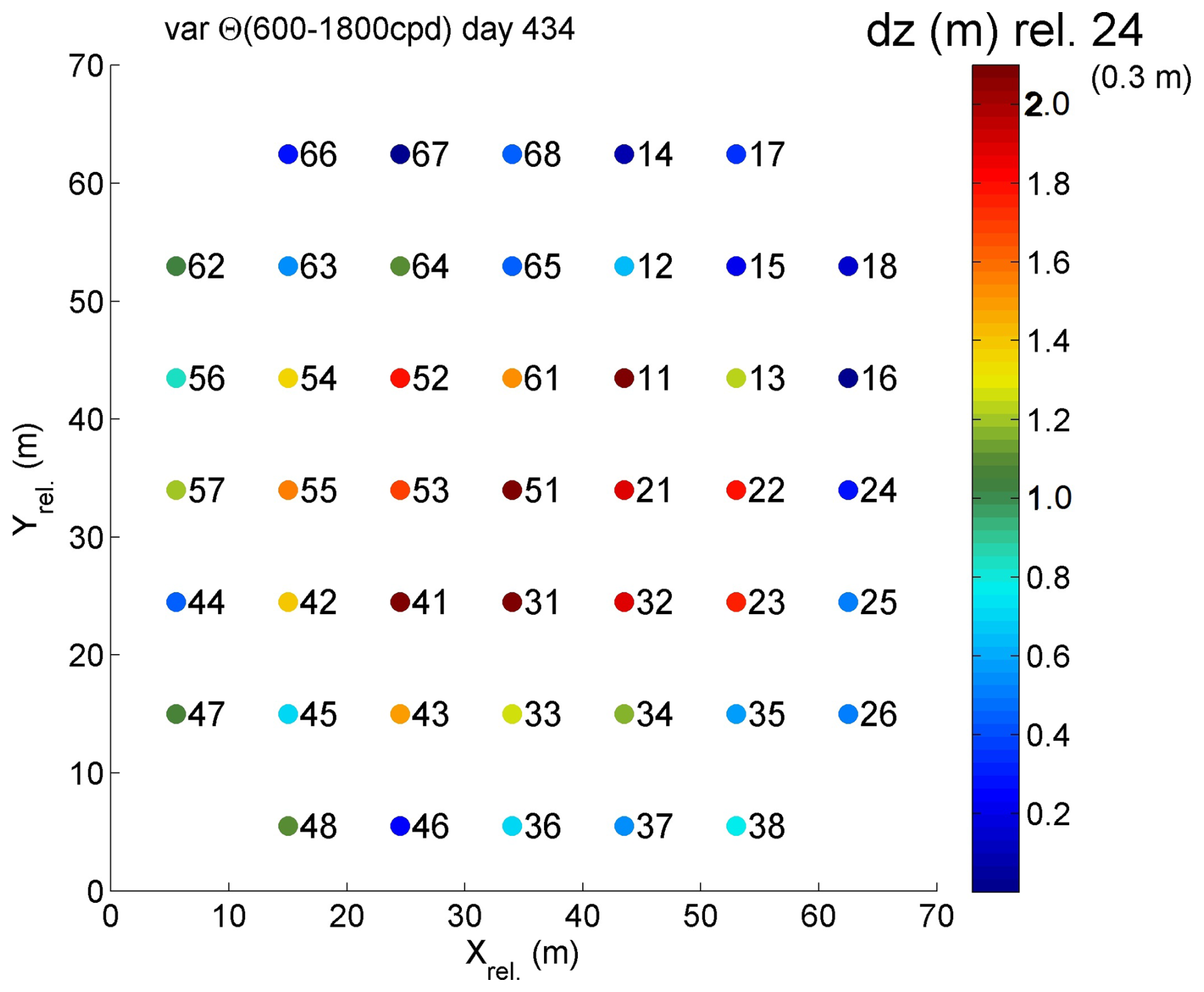
Figure B1 As Fig. 10, but for a 3.6 h short warm-water period between days 434.95 and 435.1 and relative to line 24. The temperature variance gradient is determined between positions 2 and 4 (dz=4 m) above seafloor for some smoothing.