A method for quantifying correlation in the shape of oceanographic profile data

Vertical profiles are a common type of oceanographic observation, involving measurements of a variable across a range of depths, and are widely used to identify physical and biogeochemical features of the water column. Recent studies have shown that oceanographic profiles can be represented as functional data objects, where each profile is treated as a single datum and expressed as a function of pressure. This study applies a recently developed technique, which defines a scalar correlation coefficient for functional data, to the analysis of oceanographic profiles. The method represents each profile using basis functions, whose associated weightings are termed basis coefficients, and quantifies dependence through the variability of these coefficients. An important advantage of this method is that the resulting correlation coefficient reflects similarities in overall profile shape, not just correlations between values at specific depths. Two applications of this method are explored: calculating the correlation coefficient between two different oceanographic variables, and estimating the temporal autocorrelation function of a single variable. Each application is demonstrated using two case study datasets: (1) the Coastal Endurance Washington Offshore Profiler Mooring and (2) biogeochemical-Argo floats. The first case study demonstrates how the method can be used to identify physical drivers of variability in biogeochemical profile structure. The second case study reveals regional differences in relationships between profiled variables and their temporal autocorrelation characteristics. This technique has broad potential for application to data from moorings, autonomous platforms, and ocean models, with possible use in observing system optimisation, data assimilation, and the analysis of vertically structured ocean processes.

1 Introduction

Oceanographic depth profiles describe vertical changes in the physical, chemical, and biological properties of the water column and are widely collected because they help to reveal important features like thermoclines (de Boyer Montégut et al., 2004), subsurface chlorophyll maxima (Cornec et al., 2021a) and oxygen minimum zones (Lovecchio et al., 2022). Measuring profiles of several variables simultaneously can allow for a more integrated interpretation of the vertical environment, such as assessing how biogeochemical phenomena are coupled to the physical structure of the water column (Carranza et al., 2018; Burke et al., 2023; Cao et al., 2024). Historically, ship based observations were the primary source of comprehensive profiling datasets; however they are sparse in space and time, especially in inaccessible regions. However, over the past two decades, the quantity of depth profiles has increased substantially due to the widespread deployment of autonomous observing platforms (Wong et al., 2020), many of which can measure a suite of physical and biogeochemical variables (Chai et al., 2020; Whitt et al., 2020). Furthermore, technological developments have enabled autonomous platforms to operate for long periods whilst sampling at frequencies high enough to observe small-scale processes such as turbulence (Rudnick, 2016). This rapid growth in both the quantity and diversity of profiling data highlights the need for statistical tools tailored to depth profiles to aid their analysis and improve understanding of ocean vertical structure.

Functional data analysis (FDA) provides a framework for analysing data that take the form of continuous curves, where a variable of interest is expressed as a function of an indexing variable (Ramsay and Silverman, 2005). This enables analysis of the shape of the resulting functions. Recent work has demonstrated the benefits of treating oceanographic profiles as continuous functional data objects, where depth (or pressure) serves as the indexing variable (Yarger et al., 2022; Korte-Stapff et al., 2026; Kande et al., 2024). This allows for the essence of the profile shape to be captured within each datum, alongside the numerical values. This perspective is consistent with mathematical models of the ocean’s vertical structure, which capture depth dependent interactions among key variables (Steele, 1964; Fennel and Boss, 2003; Alhassan et al., 2024). Additionally, representing profiles as functions helps mitigate sampling irregularities between profiles. Although previous studies have utilised this approach in the context of spatio-temporal modelling and interpolation (Yarger et al., 2022; Korte-Stapff et al., 2026), there are opportunities to explore more fundamental analyses through the lens of FDA. Urbano-Leon et al. (2023) developed a methodology for quantifying the variance of a functional dataset as a single value (a scalar), when previously only a variance function was used (Ramsay and Silverman, 2005). This approach involves representing each functional datum as the linear combination of a set of basis functions, whose corresponding weightings are called basis coefficients. Urbano-Leon et al. (2023) defined the variance and covariance of paired functional datasets as sums of the variances and covariances of the basis coefficients, and used these quantities to compute a scalar correlation coefficient. The purpose of this work is to present the first applications of this statistical approach to oceanographic profiles.

Correlation coefficients are commonly calculated between scalar oceanographic variables, particularly for surface data (McGillicuddy et al., 2001; Kahru et al., 2010; Fay and McKinley, 2017) or for metrics derived from profiles such as mixed layer depth or subsurface chlorophyll maximum depth (Jayaram et al., 2021; Xu et al., 2022). While relationships between full profiles have been identified (Carranza et al., 2018; Castro-Morales and Kaiser, 2012; Lovecchio et al., 2022), these dependencies have not been quantified with correlation coefficients. Autocorrelation functions (ACFs), which describe the persistence of a variable across spatial or temporal scales, provide information about the main sources of variability (Abbott and Letelier, 1998; Delcroix et al., 2005). ACFs are used in a range of applications including interpolation (Meyers et al., 1991), observing system design (Ford, 2021; Chamberlain et al., 2023; Chu et al., 2024) and data assimilation (Storto et al., 2018; Mirouze et al., 2016). Sumata et al. (2018) computed ACFs for profiling data in the Arctic, but estimated correlations by binning measurements at each depth rather than treating profiles as single datums. By computing correlation coefficients and ACFs directly from full profiles, the present approach complements existing methods and naturally incorporates profile shape.

The approach is illustrated with two case studies using simultaneously measured multi-variable profiles to explore the coupling between physical and biogeochemical variables. The first case study uses data from the Coastal Endurance Washington Offshore Profiler Mooring (CE09OSPM) (Risien et al., 2025), a daily-averaged time series of hydrographic and dissolved oxygen measurements at a single site, which makes it suitable for examining local temporal variability. While the annual cycles of these variables have been estimated (Risien et al., 2025), their seasonal strength was not quantified. The second case study comprises temperature and chlorophyll profiles from seven Biogeochemical-Argo (BGC-Argo) floats (Claustre et al., 2020), which typically collect depth profiles every 10 days while drifting with ocean currents. Previous studies have explored relationships between environmental conditions and vertical chlorophyll structure using BGC-Argo floats (Barbieux et al., 2019; Cornec et al., 2021a, b; Strutton et al., 2023), but correlations between hydrographic and biogeochemical profiles have not been reported. In this study, correlation coefficients between multiple profiled variables, as well as their temporal ACFs, were estimated for each case study dataset using the method developed by Urbano-Leon et al. (2023). In the first case study, the relationship between potential density and dissolved oxygen is quantified, with results indicating that variability in density may be driven by changes in salinity profiles. In addition, the strength of the seasonal variability in each variable is quantified. The second case study highlights that spatial variability can dominate temporal variability for mobile platforms. In summary, this study demonstrates that dependencies in vertical profile structure can be quantified using a scalar correlation framework. As the availability of profile observations continues to increase, this technique has broad potential for application across oceanography.

2 Methods

2.1 Scalar correlation for oceanographic profiles

Functional datasets are those in which each datum takes the form of a continuous curve or surface which is a function of at least one other variable. A recent development in FDA includes a method for calculating scalar-valued summary statistics, specifically the variance and correlation, for functional datasets (Urbano-Leon et al., 2023). The method is described briefly here, and a simple example is illustrated schematically in Fig. 1. Full details and proofs are given in Urbano-Leon et al. (2023). As background to the formulation below, functional data are represented as linear combinations of orthogonal basis functions, with associated weights known as basis coefficients. Basis functions are smooth reference curves that act as building blocks for reconstructing profiles. Orthogonality implies that each basis function captures an independent component of the data that cannot be reproduced by combining the others. Changes in the basis coefficients modify the values of the functional data and may also change its overall shape. Measuring the variability of the basis coefficients therefore provides a way to quantify variability in a functional dataset. Extending this to two datasets, together with the covariance of their basis coefficients, yields a natural description of dependence between the datasets.

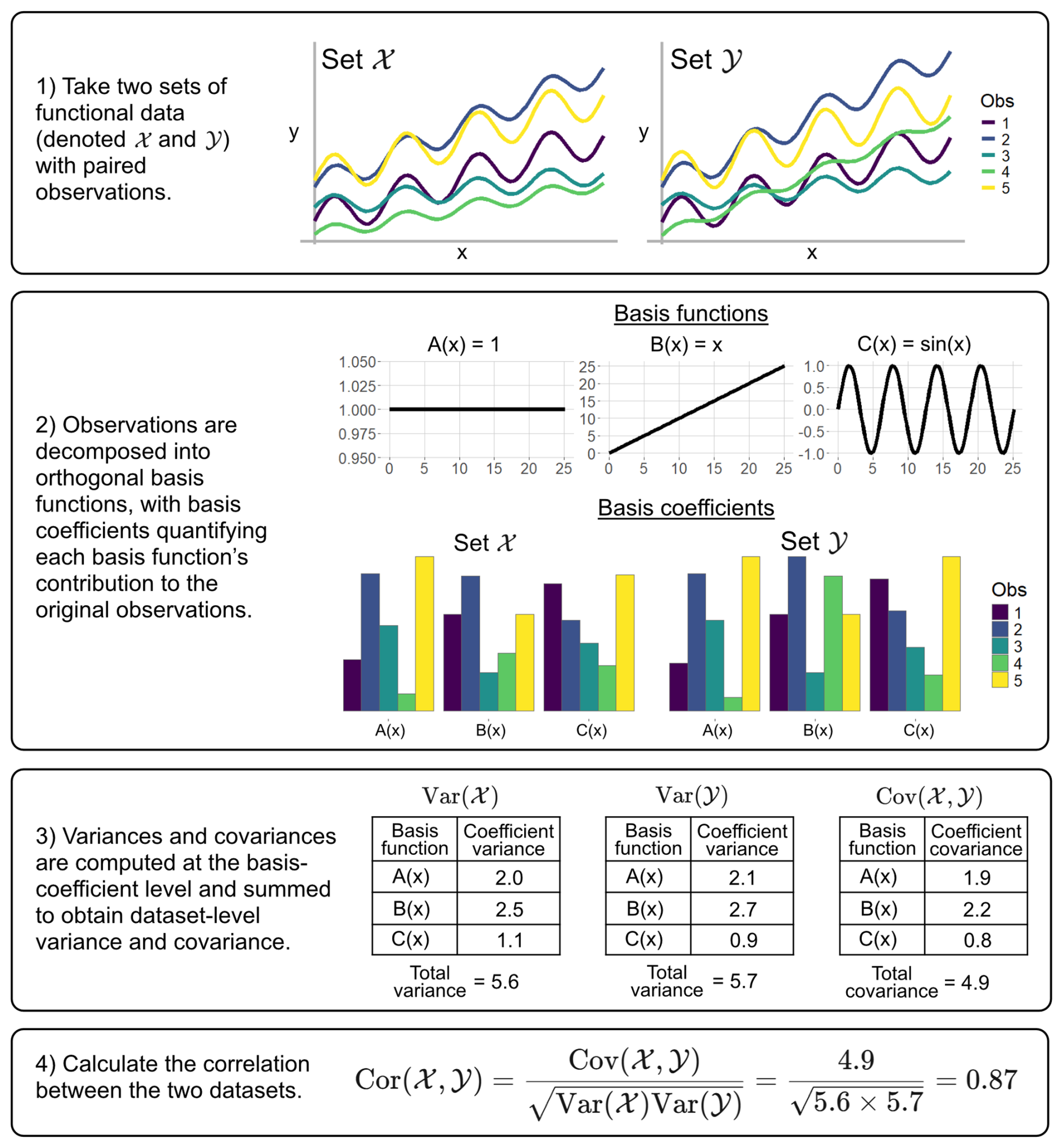
Figure 1 A visual demonstration of the method developed by Urbano-Leon et al. (2023). The figure shows the decomposition of two functional datasets, 𝒳 and 𝒴, into three orthogonal basis functions (A(x), B(x) and C(x) respectively), and the resulting calculation of their correlation. Note that scales of the bar charts were normalised.

Suppose that 𝒳 and 𝒴 are two datasets each containing n profiles (for example, paired chlorophyll and temperature profiles). Decompose each profile from 𝒳 and 𝒴 into p orthogonal basis functions with a_i,j and b_i,j denoting the coefficient of the jth basis function of the ith profile in sets 𝒳 and 𝒴 respectively. Calculation of the variability of the basis coefficients requires first computing their mean values, which for sets 𝒳 and 𝒴 are respectively given by

$$\begin{array}{}\text{(1)}& \stackrel{\mathrm{‾}}{A_j}={\displaystyle \frac{\mathrm{1}}{n}}\sum _{i=\mathrm{1}}^n{a}_{i,j},\stackrel{\mathrm{‾}}{B_j}={\displaystyle \frac{\mathrm{1}}{n}}\sum _{i=\mathrm{1}}^n{b}_{i,j}.\end{array}$$

Using the mean basis coefficients with the basis functions represents a mean function for each set, describing a characteristic profile shape. Using these mean basis coefficients, the variance of the coefficients can be calculated for each of the basis functions (denoted $V_{a_j}$ and $V_{b_j}$ respectively). The variances of sets 𝒳 and 𝒴 are then simply the sums of the basis coefficient variances $V_{a_j}$ and $V_{b_j}$ respectively.

$$\begin{array}{}\text{(2)}& {\displaystyle }\text{Var}\left(\mathcal{X}\right)=\sum _{j=\mathrm{1}}^p{V}_{a_j}=\sum _{j=\mathrm{1}}^p{\displaystyle \frac{\mathrm{1}}{n}}\sum _{i=\mathrm{1}}^n(a_{i,j}-\stackrel{\mathrm{‾}}{A_j}{)}^{\mathrm{2}}\text{(3)}& {\displaystyle }\text{Var}\left(\mathcal{Y}\right)=\sum _{j=\mathrm{1}}^p{V}_{b_j}=\sum _{j=\mathrm{1}}^p{\displaystyle \frac{\mathrm{1}}{n}}\sum _{i=\mathrm{1}}^n(b_{i,j}-\stackrel{\mathrm{‾}}{B_j}{)}^{\mathrm{2}}\end{array}$$

Similarly, the covariance between sets 𝒳 and 𝒴 is defined as the sum of the covariances of each basis coefficient C_j.

$$\begin{array}{}\text{(4)}& \text{Cov}(\mathcal{X},\mathcal{Y})=\sum _{j=\mathrm{1}}^p{C}_j=\sum _{j=\mathrm{1}}^p{\displaystyle \frac{\mathrm{1}}{n}}\sum _{i=\mathrm{1}}^n(a_{i,j}-\stackrel{\mathrm{‾}}{A_j})(b_{i,j}-\stackrel{\mathrm{‾}}{B_j})\end{array}$$

The equation to calculate the correlation between the sets 𝒳 and 𝒴 is the same for scalar data.

$$\begin{array}{}\text{(5)}& \text{Cor}(\mathcal{X},\mathcal{Y})={\displaystyle \frac{\text{Cov}(\mathcal{X},\mathcal{Y})}{\sqrt{\text{Var}\left(\mathcal{X}\right)\text{Var}\left(\mathcal{Y}\right)}}}\end{array}$$

The correlation for functional data is restricted to the closed interval $[-\mathrm{1},\mathrm{1}]$, identical to that for scalar data. Mathematically, a correlation of +1 implies that corresponding basis coefficients are perfectly positively linearly related, such that a positive change in a basis coefficient in one dataset results in a proportional positive change in the same coefficient in the corresponding observation. A deviation (from the mean function) in a specific basis component in set 𝒳 corresponds to a deviation in the same direction in the equivalent component in the set 𝒴. In contrast, a correlation of −1 represents a case where each basis is perfectly linear and negatively correlated. Specifically, this implies that any deviation in a particular component in set 𝒳 corresponds to a deviation in the opposite direction from the mean function in set 𝒴. Note that this does not imply that each pair of functions is a pointwise negative of the other, but instead they vary in opposite directions along the structural features captured by the basis coefficient. Figure 2 shows several examples of datasets containing pairs of oceanographic profiles, illustrating a range of correlation structures. In Examples 1 and 2, the profiles exhibit strong positive correlation, meaning that positive deviations from the mean in one dataset are mirrored by similar deviations in the other. Notably, Example 2 highlights that this correlation coefficient reflects dependence between deviations, rather than similarity in the overall shape of the mean profiles. In contrast, Examples 3 and 4 show negligible correlation, with variations in one profile occurring independently of the other. Finally, Examples 5 and 6 demonstrate negative correlation, where positive deviations in one dataset are associated with corresponding negative deviations in the other.

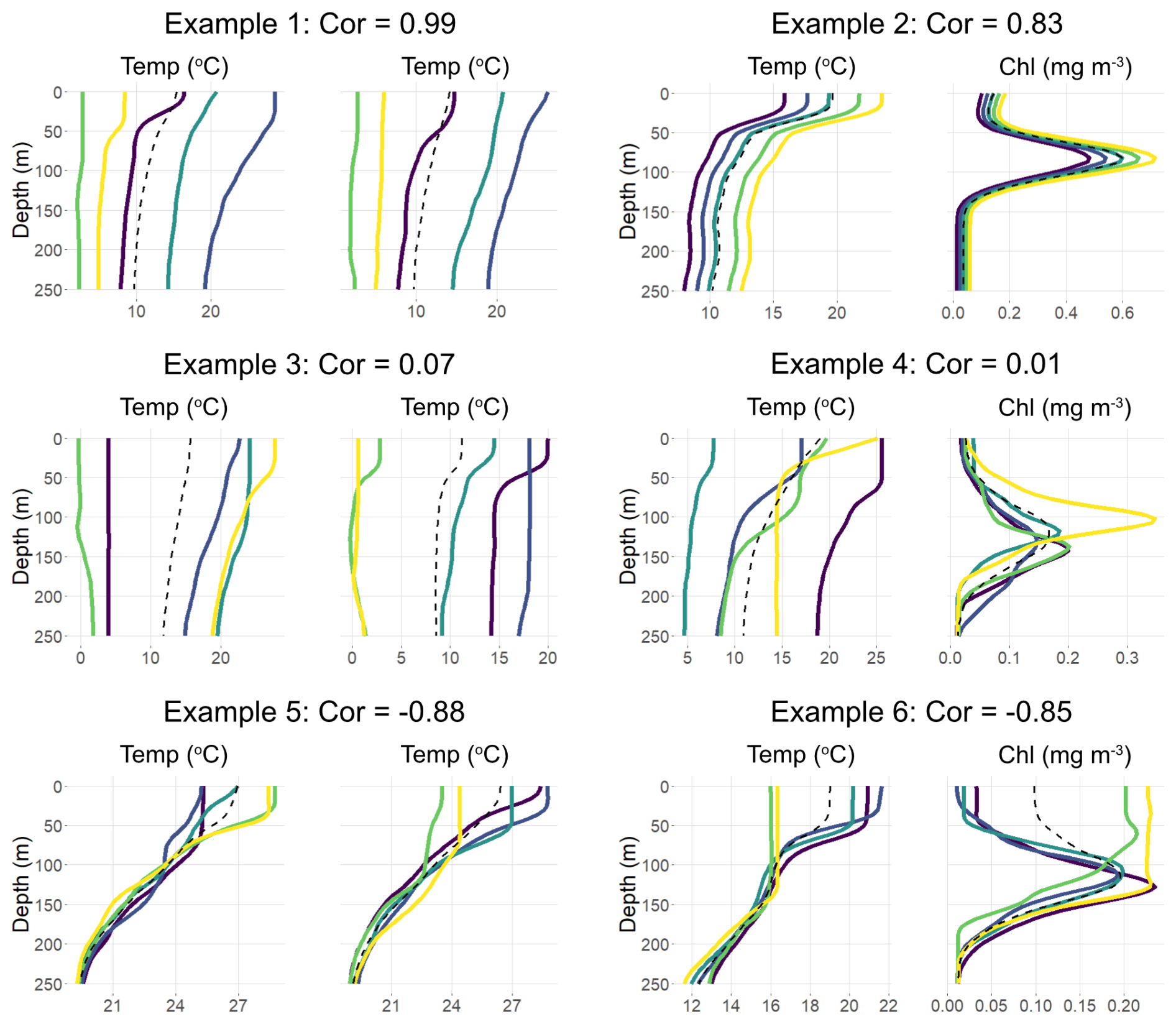
Figure 2 Six examples of paired sets of oceanographic profiles represented as functional data, together with their corresponding correlations. Colours indicate matched pairs across the two sets, and dashed curves denote the mean profiles of each set. In Example 2, the profiles were constructed to illustrate that a high correlation can arise even when the mean profile shapes differ substantially.

It is worth noting that this method could, in principle, be extended to compare sets of profiles measured over different depth ranges, although an example is not provided in the present study. This could be achieved by rescaling each range to a common interval (e.g., [0,1]) and representing the profiles using regularly spaced measurements with a consistent number of points and basis functions. The interpretation would then differ slightly, in that a deviation in one set of profiles may correspond to a deviation at a different physical depth in another set. This approach could also help identify depth ranges over which two variables are correlated, such as within the mixed layer, by iteratively repeating the analysis with modified profile segments to detect where the dependence in profile shape breaks down.

2.2 Implementation

In practice, the profiling data from each set were stored as a matrix, with each column representing a profile and each row representing a depth level. Each profile was converted to basis function coefficients using a fast Fourier transform (FFT), where the number of basis functions equals the number of depth levels in the profile (and therefore the maximum number of basis functions is equal to the number of depth levels). Fourier bases were chosen because many oceanographic profiles vary smoothly with depth, allowing compact representation by sinusoidal functions, and because they performed well in previous work on temperature time series (Urbano-Leon et al., 2023). This transformation requires complete data vectors; therefore, profiles with missing values were removed or gap-filled prior to analysis. Details of the preprocessing steps are provided in the case studies in Sect. 3. It is worth noting that this study does not explore the effect of smoothing on the computed correlation coefficients. However, the approach is expected to be robust, provided that the general shape of the profiles is sufficiently clear to allow identification of meaningful water column features. Where profiles exhibit substantial noise relative to the underlying signal, smoothing is recommended prior to computing correlation coefficients.

The FFT produces complex-valued coefficients, stored as a matrix where each row now contains coefficients associated with a different basis function. To preserve linearity for subsequent statistical calculations, the variance of each coefficient was defined as the sum of the variances of its real and imaginary components, and the covariance between coefficients as the sum of the covariances of the corresponding real and imaginary parts. This enables direct computation of variance and covariance in the transformed space, whereas some alternative basis expansions yield real-valued coefficients only. Row-wise variances were computed for each coefficient matrix and summed across coefficients to obtain dataset-level variances. Covariances were computed similarly by summing row-wise covariances between paired matrices.

To compute correlations between oceanographic variables, each data matrix contained profiles of a single variable, with simultaneously measured profiles aligned in corresponding columns. Temporal ACFs were estimated by identifying all profile pairs separated by a specified time lag. For each lag, earlier profiles formed one matrix and later profiles the other, ensuring matched dimensions and indexing. Time lags up to two years (730 d) were evaluated. All analyses were conducted in R version 4.4.1 (R Core Team, 2023). To improve computational efficiency, the search for profile pairs at each temporal lag was implemented in C++, which was substantially faster than the equivalent R implementation, and executed on a workstation with an Intel Core i5 processor. The data for both case studies and code used in the analysis are publicly available at https://doi.org/10.5281/zenodo.18164579 (Taylor and Henson, 2026).

3 Case studies

3.1 Coastal Endurance Washington Offshore Profiler Mooring

3.1.1 Dataset description

The Coastal Endurance Washington Offshore Profiler Mooring (CE09OSPM) collected high resolution profiling data from October 2014 to May 2025 at a site 60 km west of Grays Harbor, Washington. Risien et al. (2025) produced a quality controlled, and vertically gridded dataset from these mooring measurements (Fig. 3). This dataset comprises 3244 profiles – each a daily average of up to eight measurements – of temperature, practical salinity, potential density, and dissolved oxygen (DO). It was selected because of its range of physical and biogeochemical variables and its regularly gridded structure in time and depth (0.5 dbar intervals), i.e. it already had the matrix structure described in Sect. 2.2. Profiles were truncated to 40–400 m due to high rates of missing data outside this depth range. Profiles with any missing values between 40–400 m were removed. As a result, correlation coefficients between physical variables used 3178 profiles, whereas those involving oxygen used 2250 profiles. To retain all profile variability, each profile was represented by 721 Fourier basis coefficients, corresponding to each depth measurement in the restricted profiles, prior to the correlation calculations. There are some gaps in the time series due to poor weather and instrument or software failures. As a check, correlation coefficients were computed using simulated scalar data with the sample sizes described above. The resulting values differed from the theoretical correlations (in the absence of missing observations) by at most 0.02. This suggests that the correlation estimates in this case study are robust to missing data.

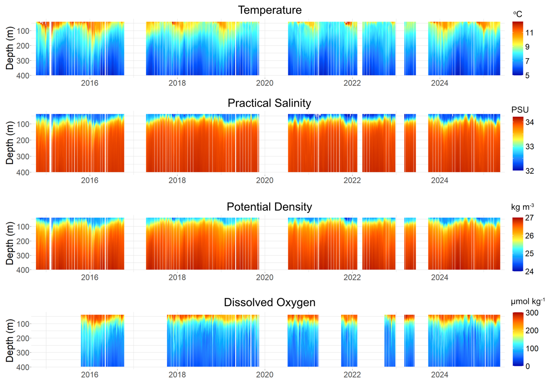
Figure 3 The dataset produced by Risien et al. (2025) comprising time series of temperature, salinity, potential density and dissolved oxygen profiles at the Coastal Endurance Washington Offshore Profiler Mooring (CE09OSPM).

3.1.2 Results

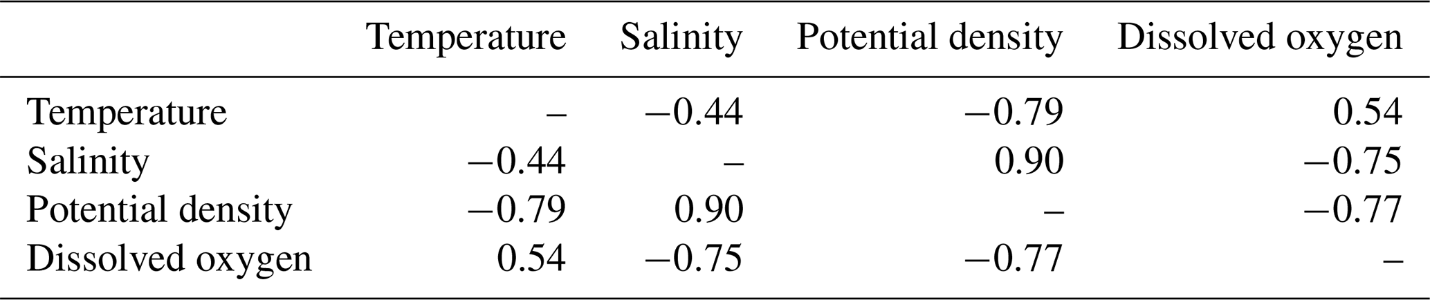
At CE09OSPM, the strongest profile correlations were observed between salinity and potential density (0.90), and between temperature and potential density (−0.79) (Table 1). Potential density and DO were also strongly correlated (–0.75), indicating that oxygen concentrations closely track the vertical structure set by mixing and stratification: as density increases at a given depth, DO tends to decrease. The weakest correlation occurred between temperature and salinity (−0.44), suggesting that density – and thus oxygen variability – is primarily driven by salinity rather than temperature. In turn, this indicates that differences in DO profile shape are governed mainly by salinity-driven changes in water mass structure, which appears appropriate after consulting the similarity in the time series of salinity and DO in Fig. 3.

Table 1 Correlation matrix between profiles of the four oceanographic variables measured at the Coastal Endurance Washington Offshore Profiler Mooring (CE09OSPM).

The temporal ACFs of all variables initially decayed exponentially, albeit at different rates, before transitioning to approximately sinusoidal patterns, reflecting seasonal cycles (Fig. 4). Temperature exhibited the strongest annual cycle, with ρ≈0.6 at a lag of 365 d and a clear sinusoidal ACF. In contrast, DO had the weakest annual autocorrelation (ρ≈0.22), indicating a less predictable interannual cycle. At short time lags, the DO ACF decayed rapidly, reaching ρ=0.6 after 18 d, whereas temperature took roughly 45 d to reach the same level. These patterns suggest that DO varies over shorter temporal scales than temperature and that its seasonal cycle is weaker and less consistent.

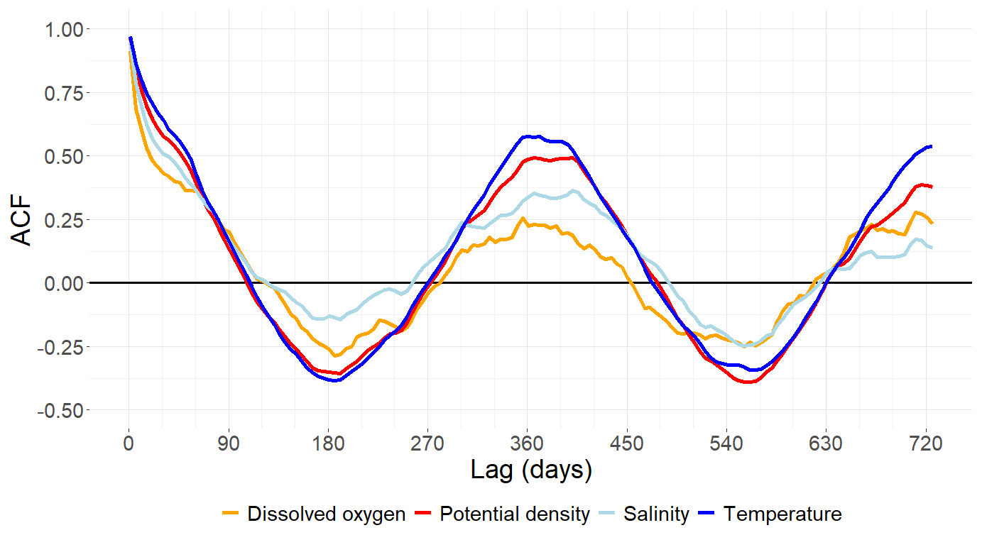
Figure 4 Temporal ACFs for four oceanographic variables measured as profiles at the Coastal Endurance Washington Offshore Profiler Mooring (CE09OSPM).

3.2 BGC-Argo float profiles

3.2.1 Dataset description

Biogeochemical-Argo (BGC-Argo) floats are autonomous platforms that measure physical and biogeochemical properties throughout the upper 2000 m of the ocean (Claustre et al., 2020). They typically profile every 10 d and drift with the currents, making them semi-Lagrangian. Here, the method was applied to temperature and chlorophyll concentration profiles from seven regularly sampling floats (WMOs 1902385, 4903365, 6901767, 5905107, 5906204, 5904021, and 6901585, shown in Fig. 5). The lifespans of floats ranged from 2.83 to 4.98 years. All profiles had undergone standard quality control prior to download (Wong et al., 2025), including correction for non-photochemical quenching of chlorophyll (Schmechtig et al., 2023). Measurements flagged as “probably bad” or “bad” were excluded. Profiles with fewer than 20 measurements between 5 and 250 m, or those not spanning at least between 20 and 230 m, were removed. Remaining profiles were regridded to 5 m intervals from 5 to 250 m using linear interpolation, then smoothed using a 15 m moving-median window. Each processed profile was represented by 51 Fourier basis coefficients, one for each regridded depth level.

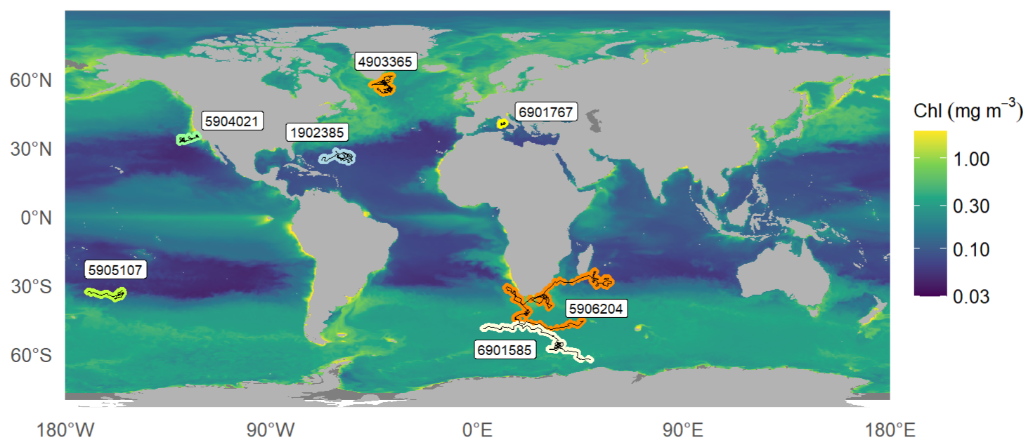
Figure 5 Trajectories of seven BGC-Argo floats used in the second case study. The background map shows the mean surface chlorophyll concentration during 2024 (E.U. Copernicus Marine Service Information, 2025).

3.2.2 Results

The correlation between chlorophyll and temperature profiles varied among BGC-Argo floats, both in magnitude and in sign (Table 2). For example, floats 4903365, 6901767, and 1902385 showed moderate positive (0.47), moderate negative (−0.42), and negligible (0.02) correlations, respectively, and these floats were located in different ocean basins. This suggests that the coupling between temperature and chlorophyll profiles may be location dependent. Floats that moved a significant distance during their lifespans (5906204, 5904021, and 6901585) also gave weak to moderate correlations, indicating that floats moving between regions may not affect the strength of correlation between chlorophyll and temperature. The negligible correlation for float 1902385 may be due to year round subsurface chlorophyll maxima despite seasonal changes in surface temperature (Fig. 6a).

Table 2 Correlation between chlorophyll and temperature profiles collected by seven BGC-Argo floats.

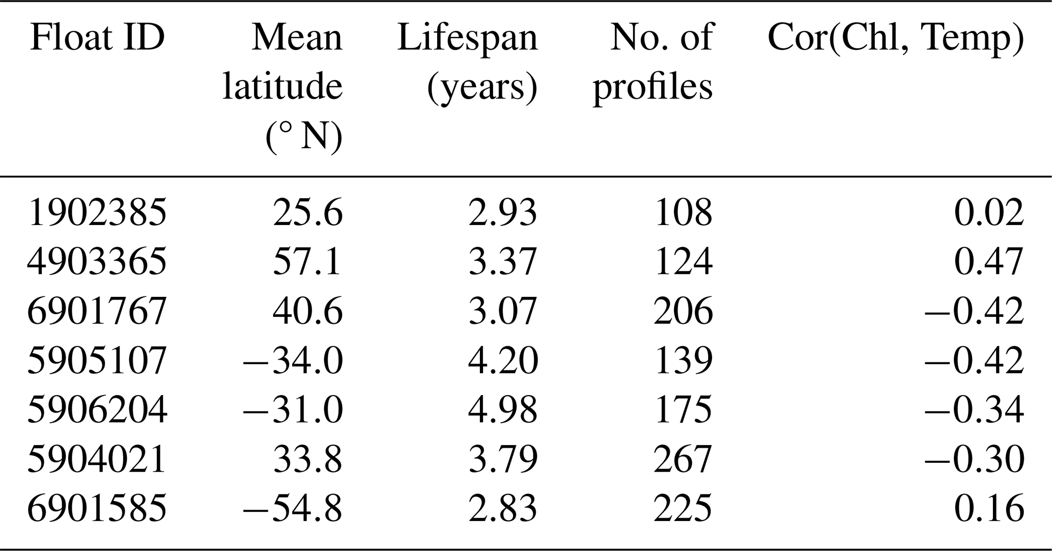
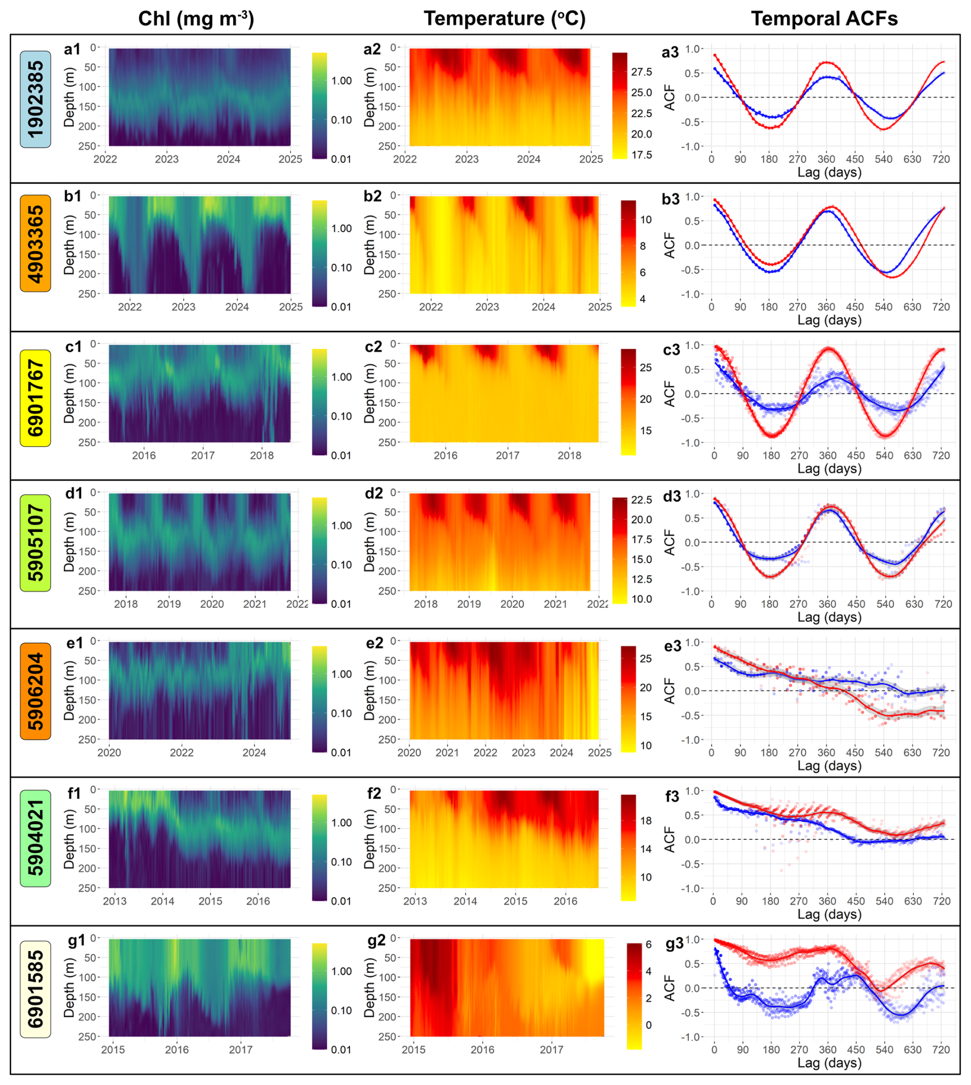
Figure 6 Temporal ACFs of chlorophyll and temperature profiles from a selection of seven BGC-Argo floats. First and second columns: semi-Lagrangian sections over the floats' lifespan of chlorophyll, and temperature, respectively. Third column: smooth curves showing the temporal ACFs for temperature (red) and chlorophyll (blue). Point opacity is lower for lags with fewer pairings and the ACFs are weighted towards points with more pairs. ACFs with scattered points indicate greater irregularity in sampling times. The colours of the boxes under the float numbers match those of corresponding profile locations in Fig. 5.

Whilst previous studies have assessed relationships between scalar-valued metrics of chlorophyll profiles and water column features (Jayaram et al., 2021; Xu et al., 2022; Zampollo et al., 2023), the results presented here instead characterise the dependence between entire profiles of chlorophyll and temperature. A key implication is that the resulting correlation coefficients naturally integrate the features of chlorophyll profiles identified by Xu et al. (2022) – including peak concentration, depth, and thickness – within a single metric. This removes the need to explicitly define and detect such features, which can be particularly advantageous when profiles lack a well-defined peak. A similar interpretation applies to temperature, where the metric implicitly incorporates properties such as surface temperature, mixed layer depth, and thermocline gradient. However, the resulting coefficient does not distinguish which, if any, specific characteristics of the profiles drive the observed correlation.

The temporal ACFs of chlorophyll and temperature profiles varied across floats (Fig. 6a–d), with four floats (WMOs 1902385, 4903365, 6901767, and 5905107) showing sinusoidal ACFs for both variables, indicating strong annual cycles. Temperature typically had a stronger seasonal cycle than chlorophyll, with correlation coefficient between 0.55 and 0.9 after a lag of one year, whereas chlorophyll had correlations between 0 and 0.6 after one year. In contrast, floats 5906204, 5904021, and 6901585 did not show sinusoidal ACFs (Fig. 6e–g). These floats travelled long distances across water masses, and their temperature ACFs remained above 0.5 for far longer than a seasonal cycle (up to a year for float 6901585). This highlights that float trajectories might influence ACF structure and decorrelation timescales, and that spatial variability might obscure seasonal signals. Over shorter time lags (<90 d), chlorophyll nearly always had a lower ACF than temperature, indicating a higher proportion of its variability occurs over subseasonal scales than temperature (Fig. 6).

4 Discussion

4.1 Profile correlation between multiple variables

The proposed method extends existing statistical tools for oceanographic profile analysis by summarising the similarity between two sets of profiles with a single correlation coefficient, analogous to the scalar-valued case. Importantly, the coefficient reflects both profile shape as well as the absolute magnitude, so dependencies in either characteristic are captured. Given the widespread familiarity with correlation coefficients, this approach provides a natural extension of scalar correlation analyses to full vertical profiles.

In an exploratory data analysis context, the method enables rapid identification of potential dependencies among multiple oceanographic variables and can inform subsequent modelling decisions. In the first case study, simultaneously measured profiles of temperature, salinity, potential density, and DO were analysed. The resulting correlation matrix (Table 1) suggests that salinity-driven density variability is a primary driver of DO variability at the mooring site. The high correlations among hydrographic variables, notably between salinity and potential density, indicate multicollinearity, implying that a model predicting DO profiles may not require all three predictors. These high correlations may be expected given that the variables are connected through well established physical relationships (Sharqawy et al., 2010). The second case study shows that the correlation between chlorophyll and temperature varies spatially (Table 2). The difference in correlation coefficients suggests that region specific analyses are required, as a single relationship may not hold across locations. In some regions, factors other than water column structure – such as nutrient availability or light – may exert stronger control on chlorophyll profiles (Cullen, 2015; Uitz et al., 2006; Cornec et al., 2021a).

4.2 Temporal autocorrelation of profiles

Oceanographers frequently investigate the temporal scales of variability in oceanographic time series, for which ACFs are a standard diagnostic tool. Previous approaches have produced ACFs for measurements collected at the surface (Meyers et al., 1991; Delcroix et al., 2005) and within specific depth bins (Sumata et al., 2018). In addition, modes of variability have been identified using empirical orthogonal functions (EOFs) (Hjelmervik and Hjelmervik, 2014; Bock et al., 2022) or by computing seasonal climatologies (Risien et al., 2025). The advantage of this approach is the quantification of temporal autocorrelation at specific time lags for time series of entire profiles. For example, in the first case study, it is shown that the autocorrelation of DO decays significantly faster than hydrographic variables for the shortest time lags (Fig. 4). When combined with weaker annual autocorrelation, this suggests that variability over short time scales is relatively more important for DO profiles, as has been shown for surface chlorophyll measurements (Prend et al., 2022). The second case study builds on this by showing that the similarity between the ACFs of two oceanographic variables can vary spatially. Furthermore, the fact that BGC-Argo floats can move substantial distances over time can lead to temporal variability being dominated by spatial variability. This is demonstrated in Fig. 6e–g where the ACFs do not display a sinusoidal curve. Visual inspection of the corresponding time series (Fig. 6e–g) confirms that that seasonal cycles are not present and sinusoidal ACFs would not be expected.

4.3 Limitations

Several caveats accompany this approach. First, it quantifies only linear dependence between sets of profiles, so non linear relationships will not be reflected in the coefficient. Second, as in the analysis of scalar-valued data, the correlation coefficient presented here does not quantify the magnitude of the causal effects between functional variables in the way that the slope of a linear regression does. Consequently, functional regression models are required to obtain this type of information (Ramsay and Silverman, 2005; Morris, 2015). Interpreting correlation scores can also be challenging because the coefficient alone gives no indication of which depths contribute to the relationship, so this method should be used alongside other tools when investigating drivers of profile variability.

The FDA approach presented here assumes that observations represent smooth functions of the indexing variable and that the sampling resolution is sufficient to capture the main vertical structure of the profile, which oceanographic profiles typically satisfy. An appropriate set of basis functions is therefore required; Fourier bases are recommended because they produce smooth function estimates while capturing variation across a range of spatial scales. However, as with any basis expansion, artefacts can arise when profiles contain sharp gradients or substantial noise. For example, truncated Fourier representations may exhibit oscillatory behaviour near sharp transitions (similar to the Gibbs phenomenon), and noisy observations can introduce small-scale fluctuations in the fitted curves. Consequently, some smoothing may be necessary prior to analysis, although excessive smoothing can artificially inflate correlation estimates. In cases where profiles from different platforms have different vertical resolutions, it is important to ensure that the analysis resolution is adequate to resolve the main differences in shape. This may require either reducing the resolution of higher-resolution profiles or interpolating lower-resolution profiles to a finer grid, depending on the vertical scale of the features being investigated.

In addition, long time lag estimates may be affected by sensor drift, which is well documented for autonomous platforms (Wong et al., 2025). Finally, the method becomes less effective for identifying long-term autocorrelation when profiling platforms move large distances, particularly between distinct oceanic regions with different hydrographic or ecological characteristics (Fig. 5).

4.4 Potential for future usage

The scalar correlation framework has broad potential across oceanographic research. It can be applied to the growing collection of datasets from moorings, profiling floats and gliders, and to model output or reanalyses to evaluate coupled physical–biogeochemical variability. As profiling data from autonomous platforms continue to expand, this method offers a way to quantify spatio-temporal autocorrelation for multiple variables and across a wide range of scales. The approach is well suited to parallelisation, making it feasible for analysing high-resolution ocean model output or global observational archives.

This framework could support observing system design for programs such as the (BGC-)Argo array (Chamberlain et al., 2023; Mignot et al., 2023; Chu et al., 2024), and extend previous decorrelation length scale studies (Mazloff et al., 2018) by incorporating full vertical profile structure. It could also be applied to high resolution glider datasets (Testor et al., 2019) to evaluate efficient sampling strategies (Patmore et al., 2024) or to compare and cross calibrate nearby platforms. Combined with satellite products such as geostrophic velocities (McKee et al., 2022), it may help assess the role of advection in driving profile variability. Alternatively, it could be beneficial to assess small scale processes through the autocorrelation of climatological anomalies.

The method could also, in principle, be used to assess reconstructed profile shapes from machine learning predictions (Sauzède et al., 2016; Chen et al., 2022; Pietropolli et al., 2023; Mignot et al., 2023). Although such models are often evaluated using pointwise metrics (e.g., RMSE), the proposed approach provides a complementary means of comparing predicted and observed profiles, potentially offering further insight into the representation of vertical water column structure. Similarly, outputs from a general circulation model (GCM) can be validated by pairing predicted profiles with the observations used to generate the model (Mignot et al., 2023), while similar analyses across multiple GCMs (Cabré et al., 2015) can help assess inter-model variability. In all cases, differences in vertical resolution between products may need to be accounted for. Another possible use is exploring potential relationships between the vertical distributions of different phytoplankton communities (Brewin et al., 2022; Miyares et al., 2024) and their preferred environmental conditions.

Future developments could include extending this approach to quantify spatial dependence in vertical profiles within spatial or spatio-temporal models (Yarger et al., 2022). The framework could also be integrated with functional regression and clustering methods to identify coherent oceanic regimes (Korte-Stapff et al., 2026; Bock et al., 2022). In addition, the autocorrelation framework could be used to fit functional time series models, such as functional autoregressive models (Chen et al., 2021).

5 Conclusions

This study applied the scalar correlation framework for functional data developed by Urbano-Leon et al. (2023) to oceanographic profiling datasets. In this framework, profile variability is represented through the variability of basis function coefficients. This enables the calculation of a scalar-valued correlation coefficient that describes the dependence of profile shape between sets of profiles. Application to two case studies containing profiling data from a stationary mooring and from BGC-Argo floats, respectively, demonstrated that the method can reveal physically meaningful relationships and spatial heterogeneity in profile dependencies. Temporal autocorrelation analyses illustrated that different variables exhibit distinct decorrelation timescales and that spatial variability can dominate temporal variability for mobile platforms.

The method has broad potential applications across oceanographic research. It can be applied to the expanding global collection of profiling observations, as well as to ocean model output, to quantify spatio-temporal variability and coupled physical–biogeochemical dynamics. Potential uses include observing system design, evaluation of sampling strategies, assessment of advective versus local variability, validation of machine learning products, and investigation of ecosystem scale decorrelation timescales. A variety of methodological approaches could be integrated with this technique, such as functional regression, clustering, spatial modelling or time series analyses. Together, these extensions would further enhance the ability to quantify and interpret variability in the rapidly growing volume of oceanographic profiling data.