Marine heatwaves across the central South Pacific: characteristics, mechanisms, and modulation by El Niño Southern Oscillation

Marine heatwaves (MHWs) are intensifying with climate change, endangering ecosystems such as coral reefs. Yet their regional characteristics and drivers remain poorly understood in many parts of the Pacific. Here we provide a comprehensive assessment of MHWs in the central South Pacific and across the five archipelagos of French Polynesia (FP; representing more than 5 million km² of maritime area, a region as vast as Europe), using sea surface temperature observations and an ocean reanalysis to investigate underlying mechanisms. MHW characteristics vary widely across the region: its northern and southern parts (the Marquesas and Austral archipelagos, respectively) experience the highest number of MHW days and the strongest cumulative intensities, especially during the warm season (November–April). In contrast, its central part (the Society, Tuamotu, and Gambier Islands) exhibits more moderate MHW characteristics. Heat budget analyses highlight the seasonally and regionally diverse mechanisms shaping MHWs. In central FP during the warm season (austral summer), most MHWs are driven by air–sea heat fluxes, while in the northern part, those driven by oceanic horizontal advection dominate. During the cold season (austral winter), more MHWs driven by horizontal advection are observed in the whole region since the thicker seasonal mixed layer reduces the proportion of MHWs driven by air–sea fluxes. El Niño–Southern Oscillation (ENSO) strongly modulates MHW occurrences: El Niño favors MHW occurrences in northeastern FP, while La Niña increases MHW occurrence in the southwest with different spatial extent depending on ENSO flavors (Central or Eastern Pacific ENSO events). This modulation arises from reduced wind-evaporation cooling with reduced wind speed, shoaled mixed layers, and enhanced horizontal heat advection, occurring primarily to the northeast of French Polynesia during El Niño and to the southwest during La Niña. These results greatly improve our understanding of MHW characteristics, dynamics and variability in this ecologically-fragile region.

1 Introduction

Extreme ocean temperature persisting in time, known as marine heatwaves (MHWs), have significant impacts on marine ecosystems and, consequently, on island communities that rely on ecosystem services, fisheries, and tourism. Their frequency and duration have increased over recent decades due to global ocean warming and are projected to continue rising in the future (Oliver et al., 2018, 2019). Developing skillful forecasts of MHWs is therefore essential to anticipate their impacts and, in turn, support effective mitigation. Such forecasts depend on a robust understanding of MHW characteristics, their mechanisms, their physical drivers, and their variability (Holbrook et al., 2020). None of these aspects has yet been studied in detail over the French Polynesia (FP) region where MHWs can lead to severe socioeconomic consequences Hédouin et al., 2020).

Some initial results regarding the mean characteristics and the dominant climate modes driving MHWs over FP can be extracted from past studies conducted at broader spatial scales, such as the South Pacific or even globally. In the South-Central Pacific, El Niño Southern Oscillation (ENSO) with its different phases El Niño (EN) and La Niña (LN) is known to be an important driver of increased and suppressed MHW occurrence (Holbrook et al., 2019, 2022) and MHW intensity (Sen Gupta et al., 2020). Additionally, the different flavors of ENSO (Capotondi et al., 2020) exhibit distinct connections with MHWs across the Pacific Ocean in terms of both intensity and frequency. Using Linear Inverse Model (LIM) data, Gregory et al. (2024) showed that these relationships vary between the Eastern Pacific (EP) and Central Pacific (CP) flavors of EN and LN. In the tropical Pacific, both MHW intensity and occurrence tend to be consistent with sea surface temperature (SST) anomalies during ENSO events, with maxima occurring in the central Pacific during CP EN events and in the eastern Pacific during EP EN events.

Regarding the mechanisms of MHWs, global studies generally rely on numerical models to estimate the main physical processes driving MHWs globally (Marin et al., 2022; Vogt et al., 2022; Bian et al., 2023, 2024). These studies aim at identifying the dominant mechanisms during MHWs among oceanic heat advection, air/sea heat flux, horizontal and vertical mixing and entrainment at the mixed layer base depending on the methods used to calculate mixed layer heat budgets during MHWs. The dominant mechanisms during the MHWs' onset and decay are region dependent (Elzahaby et al., 2022; Bian et al., 2023) and also depend on the spatial resolution of the model, which controls its ability to resolve oceanic eddies (Bian et al., 2024). This highlights the need for regional studies and observation-based studies to better understand MHWs (e.g. Schlegel et al., 2021; Elzahaby et al., 2021; Dutheil et al., 2024; Lal et al., 2025).

In austral summer (from November to April), which is the time of the year where ENSO events generally reach their peak of intensity, ENSO strongly modifies SST, ocean currents, precipitation, and wind over FP compared to climatology. Opposite influences across different parts of the country are observed depending on the ENSO flavor, due to FP's geographical position near the transition zone where ENSO SST anomalies change sign and ENSO non-linear effect on the South Pacific Convergence Zone (SPCZ) position (Vincent et al., 2011; Pagli et al., 2025a). EN (LN) events typically warm (cool) the northeastern half of FP while cooling (warming) the southwestern half, though the boundaries and intensity of these anomalies vary by ENSO flavor. During extreme EP EN events, a strong northeastward migration of the SPCZ (Vincent et al., 2011) induces enhanced precipitation and cloud cover in the northern half of FP, with intensified westerly wind anomalies. This increases Ekman pumping which deepens the thermocline in the northeastern half of FP and results in a weakening of the westward-flowing South Equatorial Current (SEC) and a strengthening of the South Equatorial Countercurrent (SECC) (Martinez et al., 2009). In contrast, CP EN events cause a more moderate northeastward SPCZ shift relative to its mean position and weaker surface winds over central FP. Moderate-to-strong LN events shift the SPCZ southwest, reducing cloud cover and enhancing trade winds, strengthening the SEC and weakening the SECC. These changes are amplified during very strong LN episodes (Pagli et al., 2025a). Overall, ENSO modulates surface ocean and atmospheric conditions, altering the large-scale background state in which MHWs may develop.

The aim of this study is to analyze in detail past oceanic MHWs over FP in order to address the following questions: What are the characteristics of past MHWs over FP and across the archipelagos? To what extent does ENSO drive, or modulate these extreme events and their dynamics? What are the local mechanisms responsible for the onset/decay of these events across the area?

Section 2 describes the data and methods used to address these questions. Section 3 presents the characteristics of past MHWs over FP, while Sect. 4 explores their modulation by ENSO. Section 5 investigates the underlying mechanisms driving these MHWs, and Sects. 6 and 7 provide the discussion and conclusions.

2 Data and Methods

2.1 Data and reanalysis data

Daily SST data were obtained from the Optimum Interpolation Sea Surface Temperature version 2 (OISSTv2) dataset, a blend of in situ and satellite observations (Huang et al., 2021), covering the period from 1981 (1 September) to 2024 (31 December) on a 0.25° grid. The mechanisms driving the MHWs detected over FP were investigated using the global eddy-resolving $\mathrm{1}/\mathrm{12}$° ocean reanalysis GLORYS12v1 (Lellouche et al., 2021), hereafter named GLORYS. In GLORYS the ocean and sea ice general circulation model is NEMO (Madec et al., 2024). Daily oceanic variables – including potential temperature, mixed layer depth, zonal and meridional currents – were analyzed. In addition, surface heat and momentum fluxes used to force the oceanic model were analyzed. GLORYS reanalysis is forced by ERA-Interim until 2019 (Dee et al., 2011) and ERA5 afterwards (Hersbach et al., 2020). Due to the known large biases in radiative fluxes at the surface in ERA-Interim, large-scale corrections were made using the NASA/GEWEX Surface Radiation Budget 3.0/3.1 product (Stackhouse et al., 2021) for shortwave and longwave fluxes (Lellouche et al., 2021). Along track altimeter sea-level anomaly, satellite sea surface temperature (AVHRR SST from NOAA) and sea-ice concentration (Ifremer/CERSAT) as well as in situ temperature and salinity vertical profiles (CORA database from CMEMS) are assimilated in GLORYS. Tides are not represented explicitly in GLORYS (Lellouche et al., 2018). Because of data assimilation, the heat and momentum budgets are not closed in GLORYS but previous studies showed its realism for analyzing MHW heat budget in the South Pacific (Dutheil et al., 2024).

MHW detection was performed using both OISSTv2 (from 1981 to 2024) and GLORYS (from 1993 to 2024). However, the mixed layer heat budget in GLORYS (see Methods) was limited to the period from 1993 to 2020 due to the forcing fields (momentum and heat fluxes) data availability. For consistency with the OISST results, GLORYS fields were regridded onto the spatial grid of the OISST dataset at 0.25° using a first order conservative remapping method.

2.2 Methods

2.2.1 MHW detection

MHWs were detected in the OISSTv2 dataset, and independently in the GLORYS reanalysis over the FP domain (165–130°W, 30–0° S) for the period 1981–2024 (respectively 1993–2024), following the method described by Hobday et al. (2016). For each product, we used the 1993–2020 period as the climatological baseline. At each grid point, a MHW was identified when daily SST exceeded the 90th seasonally varying percentile (SST^90th) (cf. Fig. S1 in the Supplement for austral summer and winter average of the threshold over FP) for at least 5 consecutive days. SST^90th was computed with a moving 11 d window to ensure enough daily SST samples for a robust 90th-percentile estimate. A 31 d moving window was then applied to remove high-frequency noise. The same filter was used for the SST climatology. Events separated by less than two days were considered as a single continuous event. Standard metrics were then calculated for each MHW, following the methodology of Hobday et al. (2016). These included the maximum, mean, and cumulative intensity, duration, onset and decline rates (defined as the mean SST rate of change from start to peak and from peak to end, respectively). The number of events and the gaps between events were also computed. MHW intensity was expressed either in absolute terms (i.e., the actual SST) or relative to the mean climatological baseline. MHWs were detected independently at each grid point; no spatial connectivity was assumed between neighboring points. Then the daily analysis of MHW occurrence across the domain was conducted to identify connected MHW areas (Lal et al., 2025). At each daily timestep, connected MHW pixels were labeled, and the area of each labeled object was calculated. For each pointwise-detected MHW, the mean and maximum spatial extent of the labeled object it belonged to were calculated over the event's duration. Throughout the manuscript, a distinction was made between MHWs occurring during the austral winter (referred to as “cold season”) and those occurring during the austral summer (referred to as “warm season”), according to the date of their peak intensity.

The severity index (S) introduced by Sen Gupta et al. (2020) was also computed on a daily basis in OISSTv2:

$$\begin{array}{}\text{(1)}& \text{Severity Index}\left(S\right)={\displaystyle \frac{\text{SST}-{\text{SST}}_{\text{clim}}}{{\mathrm{SST}}^{\mathrm{90}\mathrm{th}}-{\text{SST}}_{\text{clim}}}}\end{array}$$

where SST_clim is the SST climatology. S>1 indicates that SST exceeds the 90th percentile (i.e., SST > SST^90th), while 0 < S < 1 reflects SST values warmer than the seasonal average but not exceeding the threshold. Conversely, S < 0 denotes SST cooler than climatology. The severity of MHWs is generally described by values of S (Hobday et al., 2018). A MHW is categorized as moderate ($\mathrm{1}<S\le \mathrm{2}$), strong ($\mathrm{2}<S\le \mathrm{3}$), severe ($\mathrm{3}<S\le \mathrm{4}$) or extreme (S≥4).

In order to quantify the variability of the cumulative heat stress felt by the marine ecosystems, the daily Degree-Heating Weeks (DHW), commonly employed in coral bleaching risk assessments, were computed for each austral summer from 1981 to 2024 following Skirving et al. (2020). First, daily temperature anomalies (HotSpot) were computed relative to the local Maximum of Monthly Mean (MMM), defined as the climatological maximum of monthly mean temperatures computed over the baseline period. DHW on each day were then estimated by summing the daily HotSpot anomalies exceeding 1 °C over the preceding 12 weeks (84 d). This accumulated value was divided by seven to express DHW in °C-weeks.

Results were presented as averaged for the entire FP domain, and for each of the five main archipelagos: the Marquesas, Tuamotu, Society, Gambier, and Austral Islands. The regions associated with each archipelago, over which MHW metrics were aggregated, were defined using the official administrative geographic dataset for FP provided by the French government (datagouv; see references).

Removing a long term temperature trend (shown in Fig. S2 in the for FP region) before applying the detection method is a methodological choice as is the selection of a fixed versus a shifting baseline, both of which can influence the results and their significance (Amaya et al., 2023; Sen Gupta, 2023; Capotondi et al., 2024; Smith et al., 2025). A central question underlying these methodological choices is the definition of the “normal” state against which extreme ocean temperatures are identified. This ambiguity complicates both the definition of MHWs and the communication of MHW-related risks to the public. As a result, considerable discussion has emerged regarding MHW naming conventions and definition (Amaya et al., 2023, Sen Gupta, 2023, Smith et al., 2025). While some disagreement persists in the community regarding the definition of a MHW, it appears that both approaches are complementary, and the most appropriate depends on the specific research question to address (Smith et al., 2025). Here, we followed the guidance of Smith et al. (2025) by explicitly distinguishing MHW events identified using each approach and by clearly stating the motivation underlying the results presented. In the context of a fixed-baseline framework, retaining the long-term trend is particularly appropriate when assessing the impacts of MHWs on ecosystems or organisms with limited adaptive capacity. Conversely, when the focus is on interannual variability, climate-mode relationships, or the physical mechanisms driving MHWs, removing the trend can be advantageous for isolating these signals from the longer-term climate trends. For these reasons, the section that describes the MHWs metrics over FP was made without removing the trend (Sect. 3) and the sections analyzing the link with ENSO and the mechanisms of MHW was made with detrended SST data (Sects. 4 and 5). For Sect. 3, complementary results based on detrended SST data – where the MHW detection method and threshold computation were reapplied – are provided in the Supplement. Briefly, detrending does not alter the main results – such as differences between archipelagos, ENSO modulation, dominant mechanisms – but does slightly affect some quantitative MHW characteristics, including their duration, intensity, and onset/decline rates.

2.2.2 MHW/ENSO relationships

The link between MHWs and ENSO was examined at two levels of complexity. First, MHW occurrence across FP in all seasons was analyzed separately for EN, LN, and Neutral (N) phases, based on the Oceanic Niño Index (ONI; NOAA), using the criterion that EN (respectively LN) conditions corresponded to ONI > 0.5 (resp. < −0.5) for at least five consecutive months (see Fig. S3 for the different periods considered as EN and LN). Second, ENSO diversity was considered using the FP-specific classification developed by Pagli et al. (2025a). This classification identified six ENSO clusters based on interannual relative SST anomalies, precipitation (PR), and 850 hPa zonal wind (U850) averaged over the austral summer: three EN types (Extreme EP, Strong Mixed, and CP), one group (EPLN+N) gathering Neutral (N) and weak EP LN group (EPLN+N), and two LN types (CP and Strong Mixed). The classified years are presented in Table S1 in the Supplement (including the 2023–2024 Strong Mixed EN event, cf. Pagli et al., 2025b). For this classification, the analysis of MHW–ENSO relationships was restricted to the austral summer. MHW characteristics were composited for each of the six ENSO groups. For each ENSO cluster, both the S index and percentage of days with S≥1 were computed over the FP domain. The maximum of DHW reached over the warm season was also computed each year and composited by ENSO clusters.

2.2.3 Mixed layer heat budget and MHW category

The mechanisms of MHWs were investigated through a mixed layer heat budget analysis performed in GLORYS based on the following equation (Moisan and Niiler, 1998; Oliver et al., 2021; Dutheil et al., 2024):

$$\begin{array}{}\text{(2)}& \begin{array}{rl}\underset{\text{tendency}}{\underbrace{{\displaystyle \frac{\partial \langle T{\rangle }^{\prime }}{\partial t}}}}=& \underset{\text{Horizontal\hspace{0.17em}\hspace{0.17em}advection\hspace{0.17em}\hspace{0.17em}HADV}}{\underbrace{-\langle \mathit{U}\rangle \cdot \mathrm{\nabla }\langle T{\rangle }^{\prime }}}+\underset{\text{Air–sea\hspace{0.17em}\hspace{0.17em}heat\hspace{0.17em}\hspace{0.17em}flux}Q}{\underbrace{{\left({\displaystyle \frac{Q_{\text{net}}}{\mathit{\rho }{c}_{p}h}}\right)}^{\prime }}}\\ & +\underset{\text{RES}}{\underbrace{{\text{Residual}}^{\prime }}}\end{array}\end{array}$$

with

$$\begin{array}{}\text{(3)}& \begin{array}{rl}\text{Residual}=& \underset{\text{Horizontal\hspace{0.17em}\hspace{0.17em}mixing}}{\underbrace{\langle \mathrm{\nabla }\cdot \left({\mathit{\kappa }}_h\mathrm{\nabla }T\right)\rangle }}-\underset{\text{Vertical\hspace{0.17em}\hspace{0.17em}mixing}}{\underbrace{{\left.{\displaystyle \frac{\mathrm{1}}{h}}{\mathit{\kappa }}_z{\displaystyle \frac{\partial T}{\partial z}}\right|}_{-h}}}\\ & -\underset{\text{Entrainment}}{\underbrace{\left({\displaystyle \frac{\langle T\rangle -T_{-h}}{h}}\right)\left({\displaystyle \frac{\partial h}{\partial t}}+{\mathit{U}}_{-h}\cdot \mathrm{\nabla }h+w_{-h}\right)}}\\ +& \underset{\text{Data\hspace{0.17em}\hspace{0.17em}assimilation\hspace{0.17em}\hspace{0.17em}increments}}{\underbrace{\text{DA}}}\end{array}\end{array}$$

where ρ = 1027 kg m⁻³ is the mean density of sea water, c_p = 4187 $\mathrm{J}{\mathrm{K}}^{-\mathrm{1}}{\mathrm{kg}}^{-\mathrm{1}}$ is the specific heat capacity of seawater, κ_h and κ_z are the horizontal and vertical diffusivity coefficients in m² s⁻¹, h is the mixed layer depth in m (defined as the depth where the density increase compared to density at 10 m depth corresponds to a temperature decrease of 0.2 °C), T is the temperature in the mixed layer in K, U is the horizontal current and w is the vertical velocity component both in m s⁻¹, Q_net is the net air–sea heat flux in W m⁻². Brackets 〈⋅〉 indicate the vertical averaging from the surface to the mixed layer depth. The subscript −h indicates the evaluation of the expression at the mixed layer depth. Each term of Eqs. (2) and (3) correspond to anomalies with respect to the daily climatology (as indicated by the prime) computed over 1993–2020.

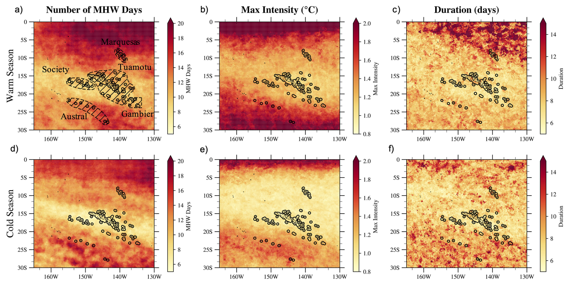
Figure 1 Median characteristics of MHWs detected over the FP region for the period 1981–2024 in the OISST dataset. The total number of days in MHW expressed in mean number of days per year, maximum intensity (°C), and event duration (days) are displayed for the warm season (NDJFMA) in (a)–(c), respectively, and for the cold season (MJJASO) in (d)–(f), respectively. The names and locations of the archipelagos are shown in (a). The black dashed areas surrounding each archipelago in (a) represent the regions used to group MHW metrics by archipelago in Fig. 2.

The net surface air/sea flux Q_net (counted as positive when entering the ocean and expressed in W m⁻²) can be decomposed as:

$$\begin{array}{}\text{(4)}& Q_{\text{net}}=\mathrm{SW}+\mathrm{LHF}+\mathrm{SHF}+\mathrm{LW}-\mathrm{SW}(-h)\end{array}$$

where SW is the net shortwave flux at the surface, SW(−h) the shortwave flux leaving at the base of the mixed layer (light vertical penetrating function being parametrized following Paulson and Simpson, 1977 for type I water, Madec et al., 2024), LHF the net latent heat flux, SHF the net sensible heat flux, and LW the net longwave radiation flux. Concerning the residual, it encompasses several processes including: the effects of data assimilation, the entrainment at the base of the mixed layer (accounting for its space–time variability, vertical advection and lateral induction), and the horizontal/vertical turbulent mixing (see Eq. 3). Errors associated with finite-difference approximations are also included in the residual term. To quantify the contribution of each term during MHW events in terms of temperature evolution, the heat budget equation was integrated in time during the MHW from the event start (t_s):

$$\begin{array}{}\text{(5)}& \begin{array}{rl}\langle T{\rangle }^{\prime }\left(t\right)-\langle T{\rangle }^{\prime }\left(t_{\mathrm{s}}\right)=& -\underset{t_{\mathrm{s}}}{\overset{t}{\int }}\langle \mathit{U}\left(\stackrel{\mathrm{̃}}{t}\right)\rangle \cdot \mathrm{\nabla }\langle T\left(\stackrel{\mathrm{̃}}{t}\right){\rangle }^{\prime }\mathrm{d}\stackrel{\mathrm{̃}}{t}\\ & +\underset{t_{\mathrm{s}}}{\overset{t}{\int }}{\displaystyle \frac{Q_{\text{net}}}{\mathit{\rho }{c}_{p}h}}(\stackrel{\mathrm{̃}}{t}{)}^{\prime }\mathrm{d}\stackrel{\mathrm{̃}}{t}\\ & +\underset{t_{\mathrm{s}}}{\overset{t}{\int }}\text{Residual}(\stackrel{\mathrm{̃}}{t}{)}^{\prime }\mathrm{d}\stackrel{\mathrm{̃}}{t}\end{array}\end{array}$$

Following Elzahaby et al. (2022), at the peak time of each MHW, the contributions (integrated in time) of each term were assessed and compared to determine which term was dominant. Events were then categorized according to the dominant mechanism: Q-MHW when air–sea fluxes dominated, HADV-MHW when horizontal advection was dominant, RES-MHW when the residual term was dominant compared to Q and HADV contribution separately as well as their sum, and Mixed-MHW when the relative difference between the Q and HADV contributions was less than 10 % of the total change of temperature from start to peak, and when their combined contribution was less than that of the residual term. For only a few events, none of the 3 terms on the right-hand side of Eq. (3) acted as positive drivers during MHW onset. These events were therefore excluded from the analysis.

To better understand the mechanisms controlling MHW onset and decay, the different terms of Eqs. (2) and (4), as well as wind (speed and direction), MLD, sea surface height (SSH) and surface oceanic currents anomalies were averaged over all MHWs occurring during the warm and cold seasons, separately. These averages were computed separately for each MHW type during the development phase, defined as the period from MHW onset to its peak intensity. During the decay phase, defined as the period from the peak to the end time, composites were constructed using all MHWs, including HADV, Q, and RES-MHWs. The full terms of Eq. (2) for these composites can be found in Appendix A (Figs. A1 and A2).

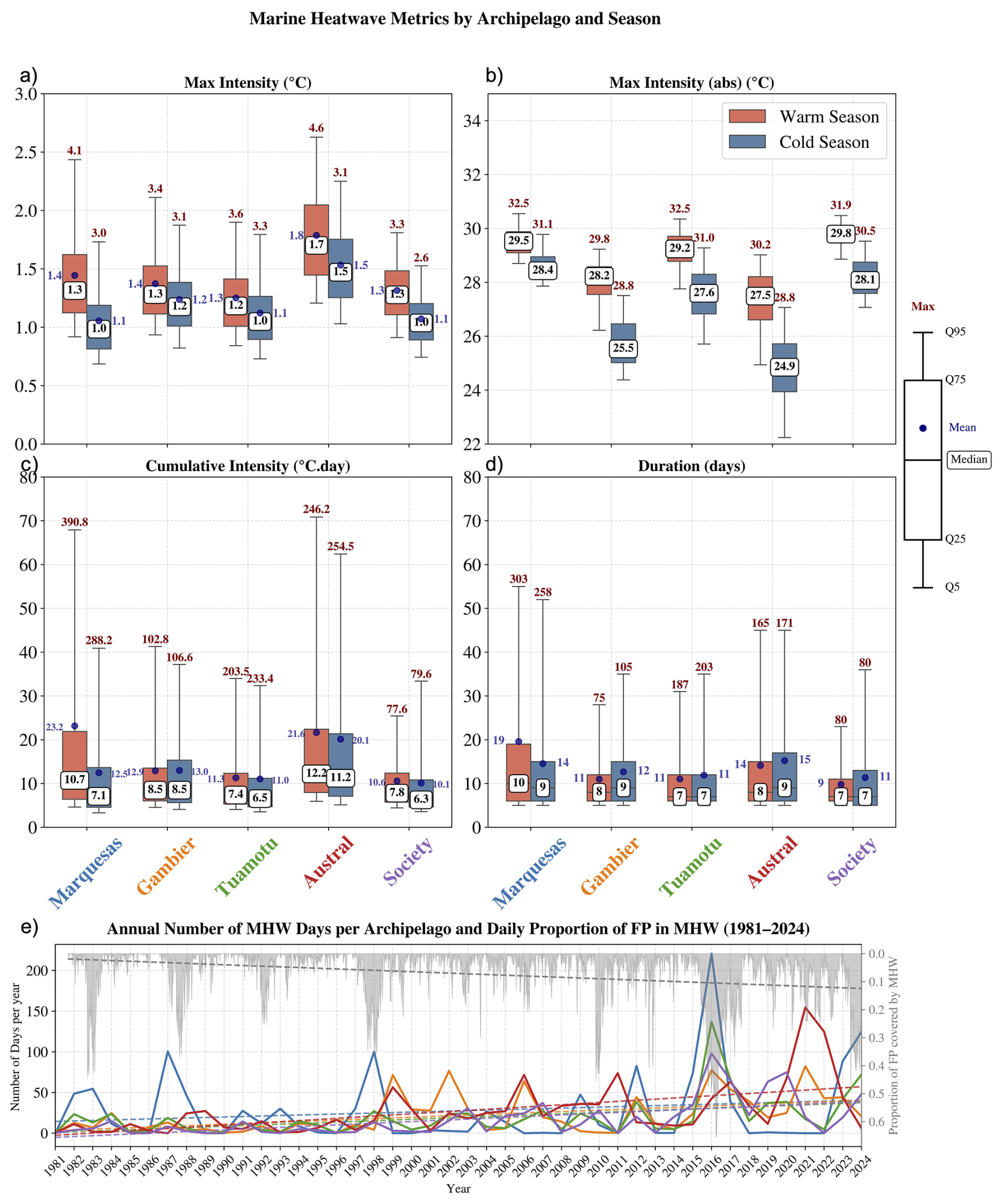
Figure 2 Panels (a)–(d) show MHW metric distributions for each archipelago area (see the black dashed area in Fig. 1a) for warm (NDJFMA, in red) and cold seasons (MJJASO, in blue). The box plots were generated from all MHW events detected at each grid point within the delimited regions around each archipelago shown on the Fig. 1a. Panels (a)–(d) show, respectively, the maximum intensity reached in each event, its absolute value, the cumulative intensity, and the duration. The whisker plot limits are indicated on the right side using a labeled box plot example. In (b), the mean value is not shown because it is very close to the median, and displaying both would reduce the readability of the plot. The difference between the mean and median maximum intensity can be assessed in (a). Panel (e) displays the annual evolution of the number of MHW days (thick lines) over each archipelago along with their linear trends (dashed lines). Line colors match the archipelago colors used on the x-axes of (c) and (d). The estimated trend slopes expressed in MHW days per decade are 6.1 d decade⁻¹ for the Marquesas (p = 0.26), 8.6 d decade⁻¹ for the Gambier (p = 0.001), 8.5 d decade⁻¹ for the Tuamotu (p = 0.002), 13.9 d decade⁻¹ for the Austral Islands (p≈ 10⁻⁶), and 10.2 d decade⁻¹ for the Society Islands (p≈ 10⁻⁵). The daily proportion of FP covered by MHWs is shown in light gray, with its corresponding linear trend indicated by a gray dashed line. The slope of the gray dashed line is 0.025 decade⁻¹ (p< 10⁻⁷).

3 MHW characteristics across the central South Pacific and FP archipelagos

Figure 1 presents the median characteristics of past MHWs – including their number, intensity, and duration – detected in the central South Pacific from 1981 to 2024 in OISST, shown separately for austral summer and austral winter. For each archipelago, Fig. 2a–d displays the distribution of these characteristics, along with absolute and cumulative intensity, to assess the level of MHW exposure across FP.

The total number of MHW days over the warm seasons of the period, expressed in mean number of MHW days per year is heterogeneous across the region (Fig. 1a). It ranges from 7 to 13 d yr⁻¹ for central regions (Society-Tuamotu-Gambier) and 13 to 18 d yr⁻¹ in the southwestern (Austral) and northeastern regions (near Marquesas) (Fig. 1a). During the cold season (Fig. 1d–f), most regions experience fewer MHW days compared to the warm season, with the exception of the Austral and Gambier region, where the number of MHW days is comparable between the two seasons.

The most intense MHWs are observed north of 7° S and south of 25° S (Fig. 1b) leading to median maximum intensity values of +1.7 and +1.5 °C in the Austral Islands during the warm and cold seasons, respectively (Fig. 2a). In the other archipelagos, median intensity values range from +1.0 to +1.3 °C. Across all archipelagos, MHWs are more intense during the warm season than during the cold season, both in terms of median and extreme values (Fig. 2a and b). Due to the large meridional extent of FP, climatological temperatures vary significantly from south to north (see Fig. S1). Absolute temperatures reached are therefore quite different between the Austral and Marquesas. In absolute terms, the most intense heat exposure is found over the Society, Tuamotu, and Marquesas archipelagos, with median values ranging from 27.6 to 28.4 °C in the cold season and from 29.2 to 29.8 °C in the warm season (Fig. 2b). The most intense heat exposure exceeds 30 °C across most archipelagos during both seasons, except in the Gambier Islands (28.8 and 29.8 °C for the warm and cold seasons, respectively) and in the Austral Islands during the cold season (28.8 °C) (Fig. 2b).

The median duration is around 7–10 d for both seasons, with longer duration for the Marquesas region over the warm season (Fig. 1c). Most MHW events are short-lived events, across all five archipelagos (Fig. 2d). Longer events are particularly frequent in the Marquesas during the austral summer, where 25 % of MHWs last longer than 19–20 d, 5 % last more than 50 d, and the longest MHWs exceed 250 d in both seasons. In the Austral Islands, the upper tail of the duration distribution is also shifted upward compared to other archipelagos, with 5 % of MHWs lasting more than 45 d in both seasons. For the others, 75 % of the distribution lies between 10 and 17 d.

Cumulative intensity varies across FP in line with intensity and duration distributions (Fig. 2c). The Austral Islands (both seasons) and the Marquesas (warm season) experience the highest cumulative intensities, with median values of 10 to 12 °C d⁻¹. In these regions, 25 % of MHWs have cumulative intensities exceeding 20 °C d⁻¹, and 5 % exceed 60 °C d⁻¹. In the Society, Gambier, and Tuamotu Islands, median cumulative intensities are 7.8, 7.4, and 8.2 °C d⁻¹, respectively. In these archipelagos, 25 % of MHWs exceed 10 °C d⁻¹, and 5 % exceed 30 °C d⁻¹ – except in the Society Islands during the warm season, where 5 % of MHWs exceed 25 °C d⁻¹.

There is an overall positive trend of the number of MHW days over FP over the period for all archipelagos, as well as the area covered by MHWs over the FP region (Fig. 2e). Also, MHW occurrence varies greatly from year to year, and not similarly in each archipelago (Fig. 2e). In the Marquesas, several years may pass with few or no MHW events, followed by years with a very high number of MHW days. In the Austral Islands, MHWs are occurring more frequently each year, although substantial interannual variability remains, with some years – such as 2021 and 2022 – characterized by a high number of MHW days. These differences led us to look at the link with ENSO (see Sect. 4).

Additional metrics, such as onset and decline rate and maximum area, are provided in the Supplement (Fig. S4). MHWs develop and decay at a comparable pace across both seasons (MHWs develop slightly faster during the warm season than during the cold season, not shown) and all archipelagos, with median growth rates ranging from 0.09 to 0.13 °C d⁻¹ and decaying rates ranging from 0.09 to 0.12 °C d⁻¹ (Fig. S4a and b). MHWs occurring in the Marquesas tend to have larger spatial extents (median of 1.7 million km² which is about 20 % of the FP maritime Exclusive Economic Zone) compared to those in the Tuamotu, Society, Austral, and Gambier Islands, where median values range from 400 000 to 600 000 km². Moreover, large MHWs (more than 10⁶ km²) are more frequently detected over the Tuamotu and Society Islands than in the Austral and Gambier Islands.

Equivalent analyses to those of Figs. 1 and 2 using the detrended MHW dataset are also available in Figs. S5 and S6. In brief, detrending the data does not alter the differences observed between archipelagos but slightly reduces MHW intensities across all regions, except in the Marquesas where the SST trend is weak and negative (Fig. S2). Detrending also reduces MHW duration across all archipelagos. Consequently, cumulative intensity is slightly reduced everywhere except in the Marquesas, where it is a bit increased. Additionally, detrending leads to a slight increase in the onset rate of MHWs.

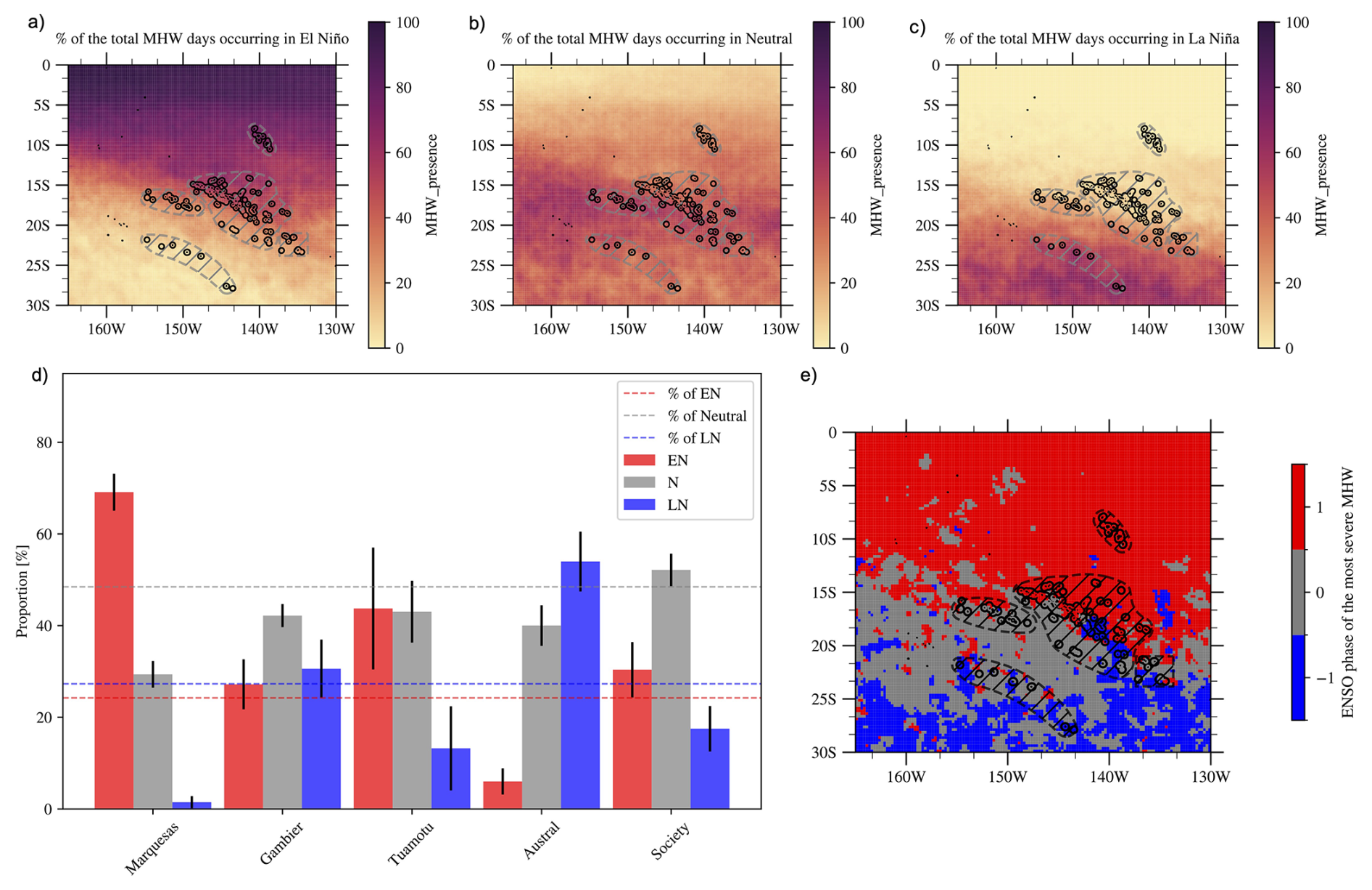
Figure 3 Proportion of MHWs occurring during different ENSO phases: El Niño (a), Neutral (b), and La Niña (c). Panel (d) shows the average percentage of MHWs associated with each ENSO phase for the five archipelagos of FP. The horizontal dashed lines indicate the proportion of El Niño (red), La Niña (blue), and Neutral (gray) days over the study period (1981–2024). Comparing the bars with the same-colored dashed lines – showing the fraction of El Niño/La Niña/Neutral days in that period – reveals how strongly ENSO modulates MHW occurrence. Black error bars indicate the spatial standard deviation of the statistics calculated across grid points associated with each archipelago area (black dashed outlines in e). Panel (e) shows the ENSO phase associated to the start time of the most severe MHW at each grid point (defined following the categories of Hobday et al., 2018, cf. Methods). SST was detrended prior to MHW detection for this analysis (similar results were obtained without removing the trend, not shown). The same figure for austral and boreal summer MHWs separately is shown in the Supplement, Figs. S8 and S9. Also, similar modulation is obtained in GLORYS over the same period (not shown).

The same analysis for MHWs detected in GLORYS over 1993–2024 is shown in the Supplement (Fig. S7). For the FP region, median values and inter-archipelagos differences are consistent between OISST and GLORYS. However some differences can be seen, detected MHWs are generally longer and weaker in GLORYS than in OISST in agreement with Pilo et al. (2019) and Chevillard et al. (2025). Despite these differences, the coherence between the products gives us confidence in the ability of GLORYS to simulate the past MHWs realistically and thus to analyze processes underlying MHWs in GLORYS (cf. Sect. 5).

4 ENSO as a driver of MHWs

We now analyse the link between ENSO and MHWs properties, and examine the modulation of MHWs by ENSO. In Sect. 4.1, we first simply separated days into El Niño (EN), La Niña (LN) or Neutral (N) conditions (without differentiating seasons, cf. Methods for identification of EN and LN periods). Section 4.2 discusses ENSO spatial diversity/flavors using the Pagli et al. (2025a, b)'s classification. MHWs analyzed here are those detected in the detrended SST of OISST (cf. Sect. 2.2).

4.1 Modulation of MHW occurrence and intensity

Figure 3a–c shows the proportion of MHW days occurring during EN, N, and LN conditions at each grid point. Using the proportion of MHW events starting in EN/LN/N instead of days does not change the conclusions (not shown). A clear spatial modulation of MHWs by ENSO emerges. During EN, MHWs are more frequent in the northeast region – from the Society and northern Tuamotu to the Marquesas – where up to 70 % of MHW days occur during EN (Fig. 3d). In contrast, MHWs are less common in the Austral islands during EN, accounting for only 5 % of MHW days (Fig. 3d). During LN, the spatial distribution of MHW shifts southwestward, with ∼ 60 % of MHW days in the Austral islands occurring during this phase (Fig. 3d). In the central region, where MHWs mostly occur during N periods (Fig. 3b), EN still enhances MHW occurrence over the Society and Tuamotu archipelagos (Fig. 3d). For the Gambier Islands, EN and LN show no significant effects (Fig. 3d). Figure 3e shows the ENSO phase associated with the start time of the most severe MHW (in terms of S, cf. Sect. 2.2) at each grid point, which closely aligns with the spatial modulation patterns described above. The most intense MHWs in the northeastern region (north and east Tuamotu and Marquesas) tend to occur during EN, while those in the southwestern region (Austral and south Tuamotu) are mostly associated with LN. In the central region (Society, west Tuamotu, Gambier), the signal is more variable, but the most severe events are triggered during neutral phases.

Similar conclusions were obtained with MHWs detected without having removed the trend in OISST as well as with MHWs detected in GLORYS over the same period (not shown). As shown in the Supplement (Fig. S8 and S9), the MHW spatial patterns modulated by ENSO revealed in Fig. 3 are exacerbated during austral summer (NDJFMA) during the peak of ENSO events but weakened during austral winter (MJJASO). We therefore focus on the austral summer season for a more in-depth analysis that includes ENSO diversity.

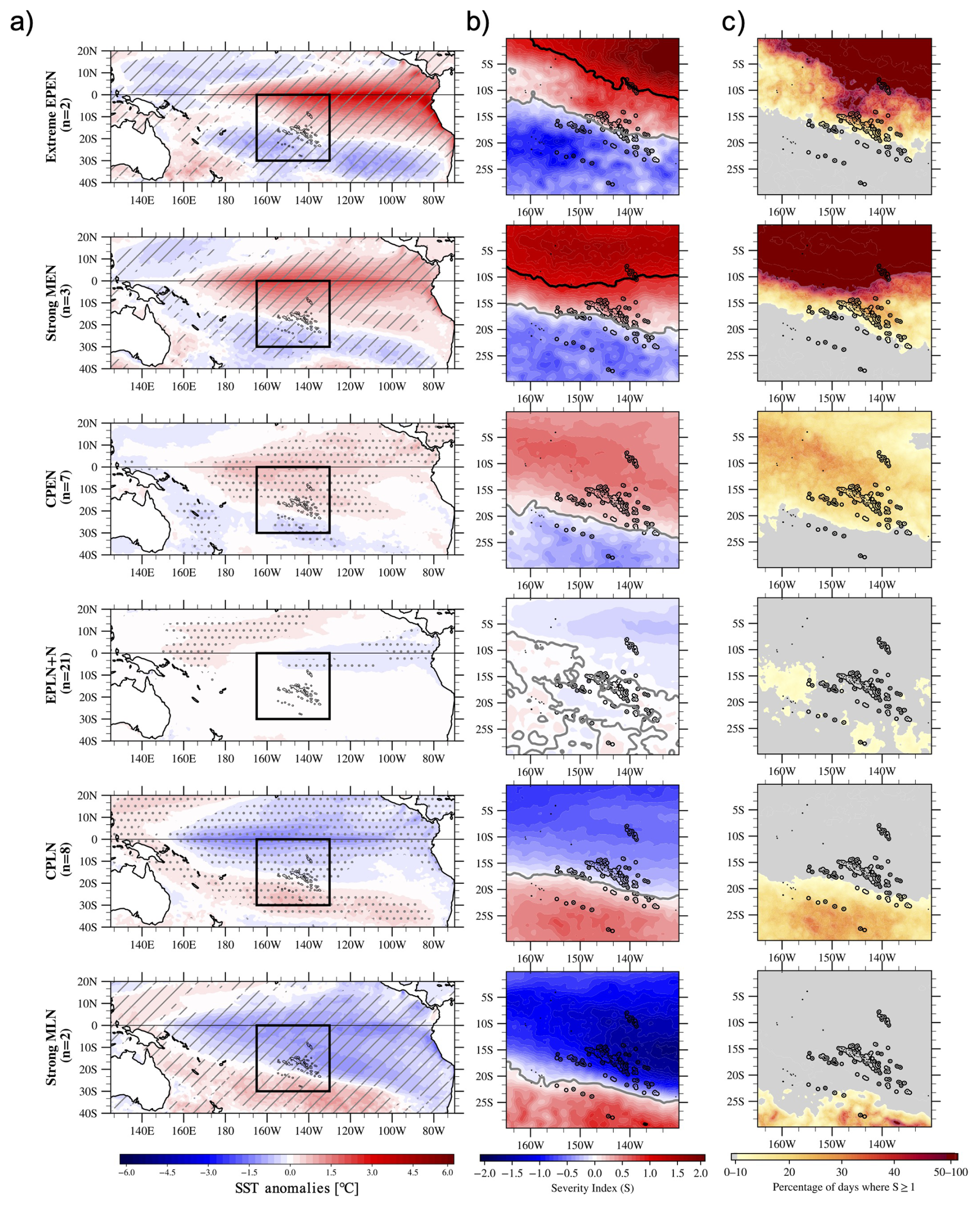
Figure 4 Composites of SST anomalies (linearly detrended) averaged over NDJFMA for the ENSO classification of Pagli et al. (2025a, b) at the Pacific scale (a). Cluster composites of S for NDJFMA are shown in (b), with isolines corresponding to S=0 and S=1 displayed in gray and black, respectively. The cluster composites of the percentage of days where S≥1 over NDJFMA is shown on (c). Gray (dark red) area corresponds to regions where 0 % to 10 % (50 %–100 %) of the NDJFMA days satisfy this criteria. In (a), dots indicate anomalies significant at the 90 % confidence level based on a two-tailed Student t-test. The number of years (n) in each ENSO cluster is indicated on the y-axis of (a). For clusters spanning two or 3 years, gray hatching marks regions where anomalies share the same sign across all years in the cluster.

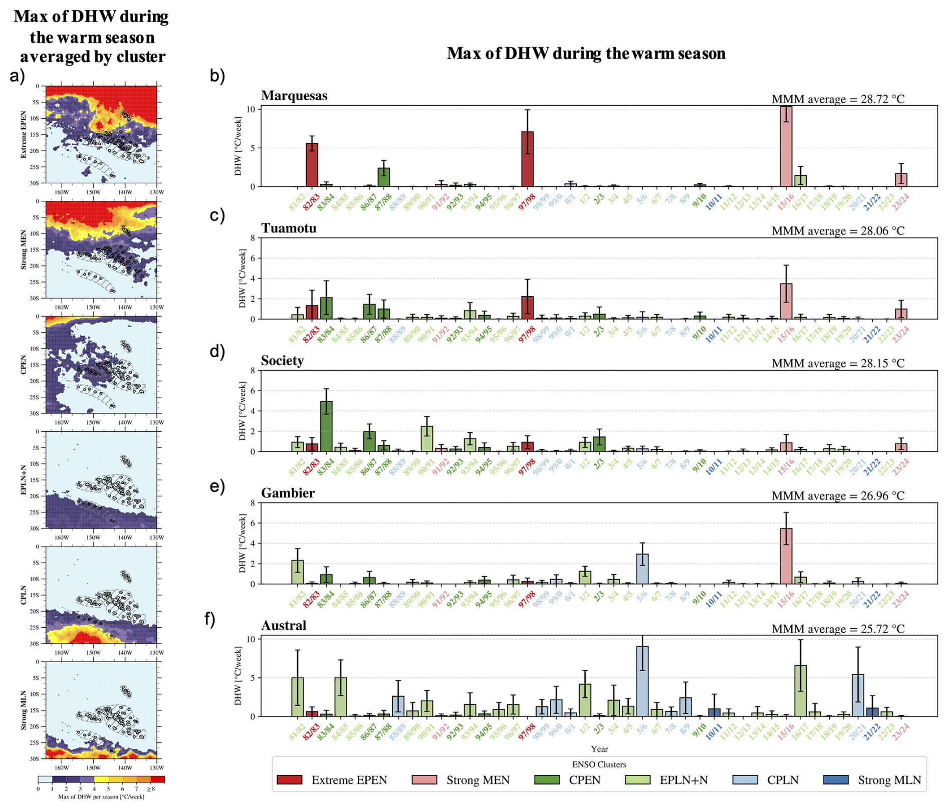
Figure 5 ENSO cluster composites of the maximum of DHW over the warm season (a) and yearly maximum of DHW averaged over each archipelago region (b–f). For each archipelago, the spatial average of the Maximum Monthly Mean (MMM) used to compute the DHW is indicated on the top right of (b)–(f). Year labels on x-axis and bars are colored by ENSO cluster. The black error bars show ± 1 standard deviation across all pixels within each archipelago area. These results were computed using detrended SST data; for DHW values based on non-detrended SST data, see Fig. S11.

4.2 Modulation of MHWs by the diverse flavors of ENSO

There is an important diversity of ENSO impacts during austral summer over FP especially in terms of SST intensities and spatial patterns (Pagli et al., 2025a and Fig. 4a). Figure 4 recalls the six ENSO clusters defined by Pagli et al. (2025a, b) at the FP scale (cf. Sect. 2.2.2 and Table S1). NDJFMA composites (average across years of each cluster) of SST anomalies at the Pacific scale (in °C) and local scale (expressed in terms of S index) are shown in Fig. 4a and b, respectively. The composite of the percentage of days where S≥1 is shown in Fig. 4c. Figure 5 highlights how the different ENSO flavors impact cumulative heat stress over the warm season at the FP scale, as depicted by DHW that takes into account the time integration of the heat stress and is recognized as an indicator of coral bleaching. The maximum of DHW reached for each austral summer averaged over years from each ENSO clusters is displayed in Fig. 5a and the same quantity averaged over each archipelago and for each year of the period is displayed in Fig. 5b–f. In the Supplement (Fig. S10), MHW intensity, duration, and the number of MHW days composited for each ENSO cluster are displayed.

Figure 4 refines the ENSO modulation of MHWs during the warm season, as introduced in Sect. 4.1 (Fig. 3). On average over the austral summer, during strong EN events, classified in strong Mixed EN (MEN) and extreme Eastern Pacific EN (EPEN) clusters, the Marquesas region and equatorward areas remain in a MHW state throughout the entire summer (90 %–100 % of MHW days, and S≥1 on average over the 6 months; see Fig. 4b and c). These MHWs are very long and intense (Fig. S10b and c), resulting in exceptionally strong cumulative heat stress over this region (Fig. 5a). Further south, MHWs are favored (0 < S < 1) in a band extending from the Marquesas to northern Tuamotu and Society Islands only (Fig. 4b and c). Over this MHW-favored area, the proportion of days with S≥1 during the warm season increases gradually from south (10 %) to north (50 %). In contrast no MHWs are detected in the far southern regions during strong MEN and extreme EPEN events. During Central Pacific EN (CPEN), all archipelagos – except the Austral Islands – experience SSTs warmer than usual (Fig. 4a), though still below the MHW threshold on average over the austral summer (Fig. 4b). These warmer SST favor MHW development and result in an average of ∼ 30 % MHW days during the warm season (Fig. 4c), with a slight increase of cumulative heat stress on average for central regions (Fig. 5a). Conversely, in the southwest, S values are on average negative (Fig. 4), indicating unfavorable conditions for MHWs. During neutral years to weak LN (EPLN+N), S anomalies across FP are weak and close to zero, only a few MHWs occur during some of these years over this region. During Central Pacific LN (CPLN-englobing most of the LN events), MHWs are favored in the southern Society Islands, extreme south Tuamotu, and the Gambier Islands, with around 20 %–30 % of MHW days over the warm season. MHWs are generally unfavored elsewhere. This leads to an increase of cumulative heat stress in the Austral Islands (Fig. 5a). Finally, during strong Mixed LN (MLN) events, MHWs are favored exclusively in the extreme south of the Austral Islands (i.e., Rapa Iti), where they are associated with strong cumulative heat stress, while unfavorable conditions prevail across the rest of FP (Fig. 5a).

Periods of increased cumulative heat stress coincide spatially with positive SST anomalies associated with the ENSO clusters. However, the magnitude of DHW can vary from year to year even for similar mean SST anomalies over the season and across archipelagos. This is because it reflects the time-integrated effect of SST anomalies and therefore the risk for coral bleaching is not systematically reached where ENSO-related SST anomalies are positive (Fig. 5b–f). In the Marquesas, very strong cumulative heat stress occured during the 1982/83, 1997/98, 2015/16, and 2023/24 El Niños (extreme EPEN and strong MEN) while 1991/92 (a strong MEN) was comparatively associated with weaker cumulative intensity (Fig. 5b). We can note also that 1987/88 (CPEN) produced a strong heat stress over the Marquesas. In the Tuamotu, the same years in addition to 1983/84, 1986/87 (CPEN) are linked to the highest cumulative heat stress (Fig. 5c), but with lower cumulative heat stress than in the Marquesas. Interestingly, the 1991/92 strong MEN event, despite being extreme for FP in terms of SPCZ displacement and tropical cyclone activity (Vincent et al., 2011; Pagli et al., 2025a, b), was not as intense in terms of MHWs over the Marquesas and Tuamotu. In the Society archipelago, 1983/84, 2009/10, 2002/03 (CPEN) and neutral years 1990/91, 2016/17 (EPLN+N) correspond to the strongest DHW values (Fig. 5d). While strong MEN and extreme EPEN years also produce considerable cumulative intensities in this region, they are not the highest, highlighting that the strongest EN events (as defined on a global scale) do not always correspond to the most severe impacts over FP. In the Gambier Islands, both EN and LN events can produce significant cumulative heat stress (2005/06 CPLN and 2015/16 strong MEN) during the warm season (Fig. 5e), with no consistent influence of specific ENSO clusters on the cumulative heat stress. This aligns with the unclear ENSO modulation highlighted for the Gambier Islands in Fig. 3. In the Austral Islands, the strongest cumulative heat stress are observed in 1988/89, 2005/06 and 2020/21 LN years, particularly CPLN events.

These conclusions were drawn from analyses based on detrended SST data, aiming to isolate the ENSO imprint on cumulative heat stress over FP. However, when using the non-detrended SST data – which reflects the total heat stress exposure experienced at the surface – the maximum DHW values over the warm season for years occurring after 2000 are amplified over the Tuamotu, Society, and Gambier archipelagos (Fig. S11) especially in 2015/16 (strong MEN) that has been associated with massive wide coral bleaching over FP (Hédouin et al., 2020) and more recently in 2023/24 (strong MEN).

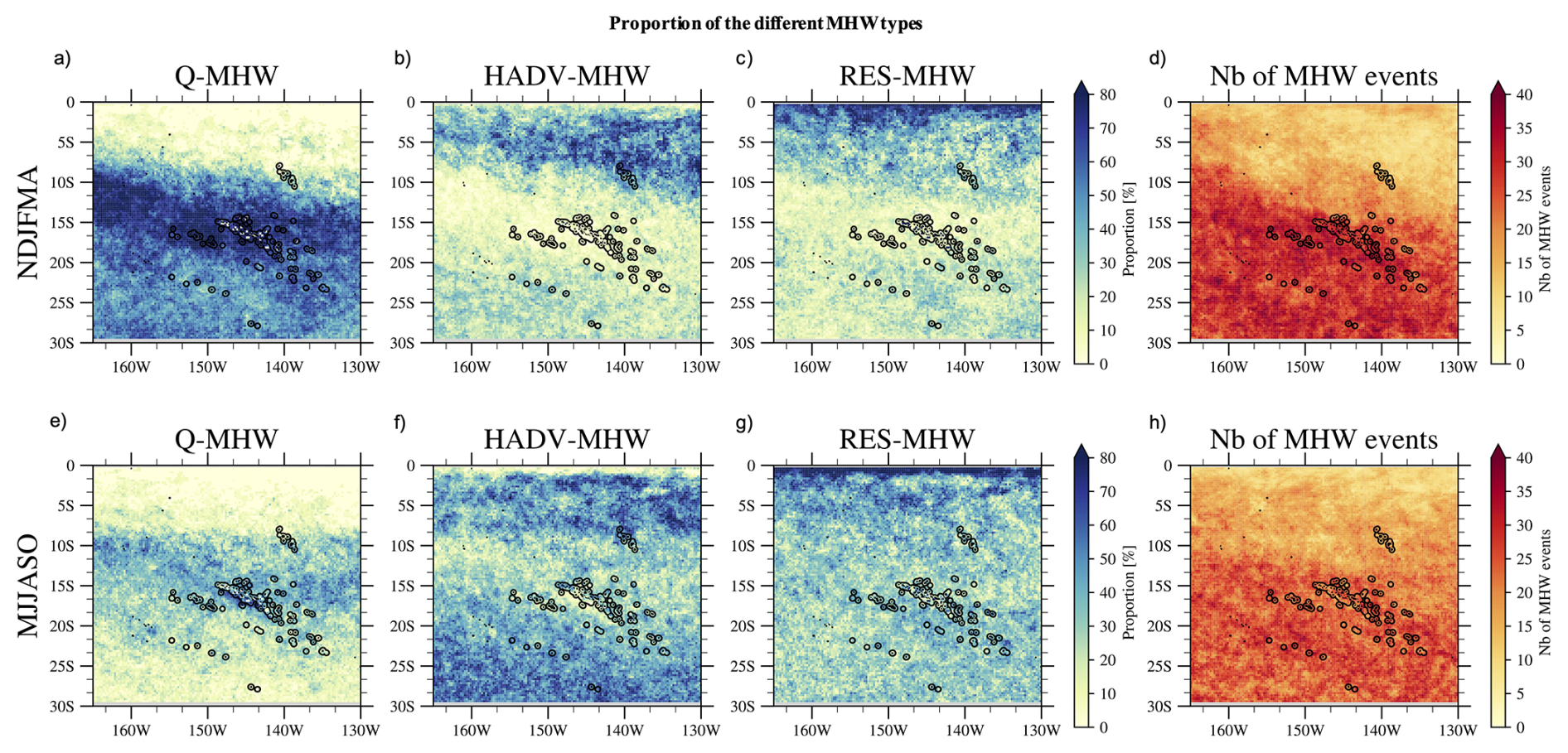
Figure 6 Proportion of the different MHW types for all events detected in austral summer and austral winter separately (d, h) in GLORYS, during the 1993–2020 period. Panels (a) and (e) show the proportion of Q-MHWs in austral summer and winter, respectively; (b) and (f) show HADV-MHWs; (c) and (g) show RES-MHWs. Mixed events are not shown, as they represent only a small number of cases.

5 Physical mechanisms generating and dissipating MHWs over 1993–2020

5.1 MHW development

In this section we investigate the physical mechanisms of the MHWs in the GLORYS oceanic reanalysis (over the 1993–2020 period, see Methods in Sect. 2.2.3). We examined the dominant local mechanisms of MHWs development across the territory for austral summer and winter separately (Fig. 6) – focusing on air–sea surface heat fluxes, horizontal advection, and residual terms (see Eq. 2). The residual term consisted mainly of the vertical/horizontal mixing and entrainment at the bottom of the mixed layer plus implicit heat sources/losses due to the assimilation in GLORYS (see Eq. 3). Also, because the vertical mixing may be poorly represented in GLORYS (due to the lack of explicit tidal forcing) and because the magnitude of the data-assimilation increments is unknown here, interpreting in detail this residual is beyond the scope of this study.

MHWs are driven by different mechanisms depending on the region and the season (Fig. 6), and a strong differentiation appears at about 10° S. During austral summer, MHWs are primarily driven by air/sea fluxes in most archipelagos south of 10° S, especially in the central regions (Society and central Tuamotu), accounting for 70 %–80 % of total events (Fig. 6a). HADV-MHWs and RES-MHWs represent 0 % to 30 % of the total events except for MHWs occurring in the equatorward region, north of 5° S/10° S (Fig. 6b and c). Here, HADV-MHWs dominate and account for 60 %–70 % of the events south of 2° S. The residual becomes dominant in a thin equatorial band due to the particular dynamics of the region with notably the equatorial upwelling (e.g. Deppenmeier et al., 2021). During austral winter, the proportion between MHWs types is more balanced in central regions with a slight dominance of Q-MHWs compared to HADV-MHWs and RES-MHWs (Fig. 6e, f, and g). HADV-MHWs proportion increases across the southern subtropical region (south of 20° S) compared to summer accounting for more than 60 % of total events. RES-MHWs proportion slightly increases across FP in winter compared to summer too. Following our classification criteria (cf. Sect. 2.2), mixed-MHW were almost never defined over both seasons (not shown).

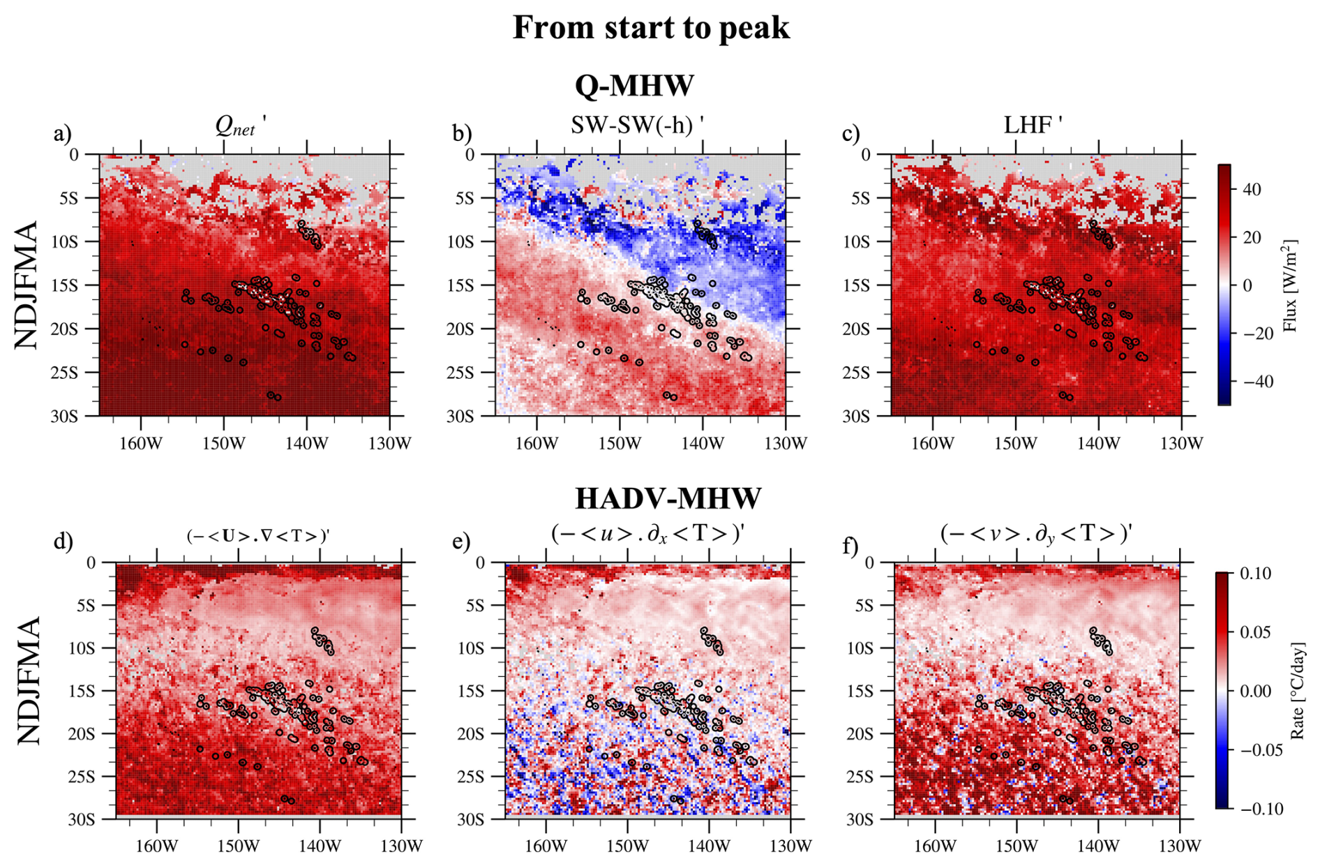
Figure 7 Composites of the net air–sea heat flux (and its dominant components: $\mathrm{SW}-\mathrm{SW}(-h)$ and LHF) for Q-MHWs and of the horizontal-advection term (and its decomposition into zonal and meridional components) for HADV-MHWs, for events peaking in the warm season (NDJFMA), averaged over the onset-to-peak period (cf. Sect. 2.2.3). Panels (a)–(c) show Q-MHW composites of (a) net air–sea heat flux Q_net (b) the net shortwave flux stored in the mixed-layer ($\mathrm{SW}-\mathrm{SW}(-h)$), and (c) LHF anomalies. Panels (d)–(f) show HADV-MHW composites of (d) horizontal advection anomalies and its (e) zonal and (f) meridional components. In each panel, the composite corresponds to the averaged across all MHWs of the corresponding type (Q-MHW or HADV-MHW) detected at each grid point.

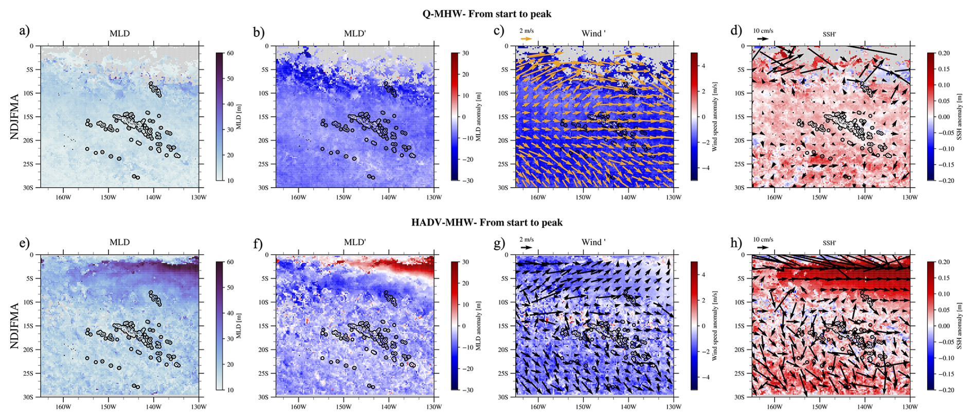
Figure 8 Conditions from start to peak of Q-MHWs (upper panels a–d) and of HADV-MHWs (lower panels e–h). MLD (a, e), MLD anomalies (b, f), 10 m-wind (speed and direction) anomalies (c, g), and SSH with oceanic currents averaged over the upper 0–30 m (d, h) for MHWs in NDJFMA. Anomalies are relative to the mean seasonal cycle computed over the whole period (1993–2020).

We now look at the mechanisms of MHW development for Q-MHWs and HADV-MHWs separately. For each MHW type, the terms in Eq. (2) were averaged from start to peak at each grid point and then composited over all events for austral summer and winter separately (Fig. A1). Only the results for the austral summer MHWs are presented in this section and those for austral winter MHWs are available in Appendix A. The standard deviation associated to the mean composites presented in Figs. A1 and A2 are presented, respectively in Figs. S12 and S18. Because Q-MHWs are, by construction, dominated by the air–sea heat budget term contribution, we focus on Q_net and its leading components, shown in Fig. 7a–c. Conversely, since HADV-MHWs are driven by horizontal advection contribution, we focus in Fig. 7d–f on the horizontal heat advection term and its zonal and meridional components. MLD (full field and anomalies), wind, SSH, and surface-current anomalies are shown in Fig. 8. These results for austral winter are available in the Supplement.

Q-MHWs

The Q_net anomalies driving Q-MHWs development are dominated by LHF anomalies (Fig. 7a–c). Anomalously weak surface winds (Fig. 8c) reduce evaporation, thereby warming the mixed layer. The net SW anomalies in the mixed-layer play a secondary role but still modulate Q_net during Q-MHWs onset in summer, with a spatially complex pattern (Fig. 7b). In the northeast, where most events occur under EN, negative net SW anomalies in the mixed layer tend to damp Q-MHWs development. They are negative because incoming SW anomalies are weakly positive or negative (Fig. S13b) due to enhanced convection during EN (Pagli et al., 2025a) and thus do not offset the increased SW loss through the mixed-layer base (Fig. S13c) caused by a shoaled mixed layer under anomalously weak winds (Fig. 8b and c). In the southwest by contrast, where MHWs are favored during LN, net SW anomalies generally reinforce the warming during the onset of the event, consistent with clearer skies and enhanced incoming SW (Fig. S13a–c) typically seen during LN due to anomalously dry conditions over austral summer (Pagli et al., 2025a).

Although air–sea flux anomalies account for most of the variability in the $Q_{\text{net}}/\left(\mathit{\rho }{c}_{p}h\right)$ term of Eq. (2), mixed-layer shoaling during onset (Fig. S15e) slightly increases the air/sea flux-term warming. In other words, a shallower mixed layer heightens its sensitivity to flux changes. Still, this effect is minor compared with the flux anomalies themselves (Fig. S15c). Horizontal advection does not exhibit a strong and systematic contribution for Q-MHWs during onset, as indicated by the noise present in HADV-MHWs composite during MHW development (Fig. A1c).

Results are broadly similar across seasons (Figs. A1e–h, S14a–c, and S13d–f). During austral winter – when the seasonal mixed layer is thicker – the required LHF anomalies, and thus the wind-speed anomalies needed for Q-MHWs to develop, are larger than in austral summer (Fig. S17a–c). This also explains why Q-MHWs are more frequent in austral summer than in austral winter (Fig. 6a and b). Also, in winter, SW variations during MHW development are highly event-dependent with no clear pattern on the composite shown in Fig. S14b. They can either reinforce or damp the warming associated to reduced evaporation (Fig. S14a–c).

HADV-MHWs

North of 10° S (but south of 3° S, out of the equatorial wave guide) – where most HADV-MHWs occur during EN (cf. Figs. 3 and 4) – both zonal and meridional heat advection contribute (Fig. 7d–f). The warming during the onset is associated to eastward current anomalies that transport the climatologically warmer waters from the west (Fig. 8h, $u^{\prime }\cdot {\partial }_x\stackrel{\mathrm{‾}}{T}$ in the ${\mathit{U}}^{\prime }\cdot \mathbf{\nabla }\stackrel{\mathrm{‾}}{T}$ term, Fig. S16g and h). In addition, the EN–enhanced SST gradient is advected by the mean circulation to higher latitudes, fueling HADV-MHWs' onset south of 10° S and up to 20° S (${\mathit{U}}^{\prime }\cdot \mathbf{\nabla }T$ term, Fig. S16d–f).

Moving southward, the signal becomes noisier, but meridional advection shows the most systematic warming during the development stage (Fig. 7f). This arises from persistent southeastward anomalous currents that can be forced directly by wind anomalies (Fig. 8g and h) and/or from geostrophic adjustment and/or from anomalous circulation linked to westward-propagating anticyclonic eddies (positive SSH, Fig. 8h; the composite method, done for MHWs at each grid point separately, smooths out eddy patterns, with only their SSH contribution during the MHW's onset at the grid point being visible), which likely also contribute to the noise seen in Fig. 8h.

Air–sea flux contributions during HADV-MHWs are less systematic as shown by the noise present in the composite in Fig. A1j, sometimes reinforcing the advective warming and sometimes damping it from one event to another. Nevertheless, in the Marquesas – where most events occur under EN – the net air/sea heat flux term tends, on average, to damp the MHW development (Fig. A1j). Southwest of the Marquesas, over other archipelagos, the air/sea flux term generally provides a slight warming, though with strong event-to-event variability (Fig. A1j). Conclusions about the onset mechanisms of HADV-MHWs are very similar in austral winter (Fig. A1m–p).

The residual term contribution to MHW onset composited for Q-MHWs and HADV-MHWs presents a strong inter-event variability and is hard to interpretate here (Fig. A1d, h, l, and p). On average, for MHWs occurring north of 10° S, the residual term contributes to the warming of the mixed layer during the MHW onset for both Q- and HADV-MHWs and over both seasons. This may be linked to reduced vertical mixing caused by the weaker winds and shallower MLD observed during the MHW development (Figs. 8b, c, f, g and S17b, c, f, g).

RES-MHWs constitute a substantial fraction of events over FP (Fig. 6c and g). Figure A1q–x shows the composites of the different terms of Eq. (2) during their onset. By construction, their development is driven by the residual term which may be dominated by vertical processes (mixing and entrainment), while contributions from air–sea fluxes and horizontal heat advection are highly variable from event to event and show no systematic pattern.

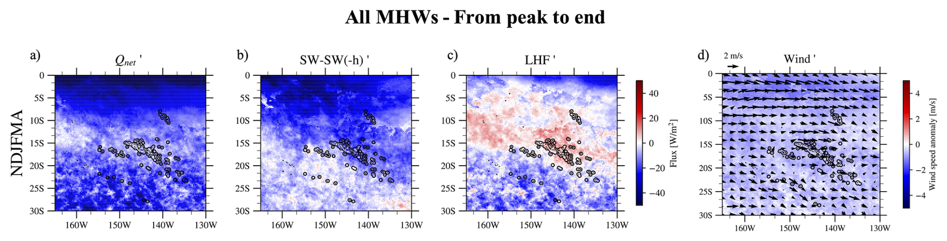
Figure 9 Composites of the net air–sea heat flux (and its dominant components) as well as surface wind anomalies averaged over the decay period i.e. from peak to end (cf. Methods) for all MHWs peaking in austral summer. Panels (a)–(c) show MHW composites of (a) net air–sea heat flux Q_net (b) the net shortwave flux in the mixed-layer ($\mathrm{SW}-\mathrm{SW}(-h)$), and (c) LHF anomalies. In each panel, the composite is averaged across all MHWs (without distinguishing by type as done during the onset period) detected at each grid point.

5.2 MHW decay

We now investigate the decay stage (peak to end) of MHWs over FP. As the classification into different MHWs types has been solely designed for the developing phase (classification criteria applied regarding the terms contribution integrated from onset to peak time, cf. Sect. 2.2.3), we used all MHWs together to study the decaying stage of MHWs (after verifying that decaying mechanisms do not significantly differ between MHWs types).

In austral summer, the transition from onset to decay (Fig. 9a and d) is dominated by cooling from the air–sea heat-flux budget term of Eq. (2) (Fig. A2). It is mainly due to negative Q_net anomalies that are mainly explained by the anomalies of the net SW in the mixed-layer in the north and of surface LHF in the south (Fig. 9a–c). Over the northeastern half of FP, it is the negative incoming SW anomalies that explain the most the cooling of mixed-layer temperature while LHF' continues on average to warm but with a strong inter-events variability. In the southwestern half, it is more systematically the cooling due to negative LHF anomalies i.e. increased evaporation that causes the decaying of MHWs. This can be due to increases in wind speed and/or SST or to a decrease in air moisture above the ocean surface (a drier air mass increasing evaporation). When looking at the composite of the wind speed anomalies for the MHW decay (Fig. 9d), these are still negative, but less than during onset, meaning that MHW warm SST and/or decrease in the surface atmosphere moisture may play a role.

In austral winter, the role of SW anomalies weakens and on average MHW decay is caused mainly by negative LHF anomalies that are more systematically associated to positive or neutral wind speed anomalies (Fig. S19), with possibly also a role of warm SST.

During MHW decay, the residual term is more spatially coherent and exhibits less noise (Fig. A2d and h) than during the onset for Q- and HADV-MHW types (right column of Fig. A1). In austral summer, it produces anomalous warming of the mixed layer; in austral winter, it warms north of ∼ 10° S and cools south of ∼ 15° S. The nature of the residual is complex and can result from different processes. The ability of their parametrization in GLORYS and the increments of data assimilation vary in space and time. Our approach (heat budget not completely closed in a reanalysis) does not allow us to interpret more in depth this residual term. Modeling approaches capable of accurately resolving this term could enhance our understanding of the underlying processes.

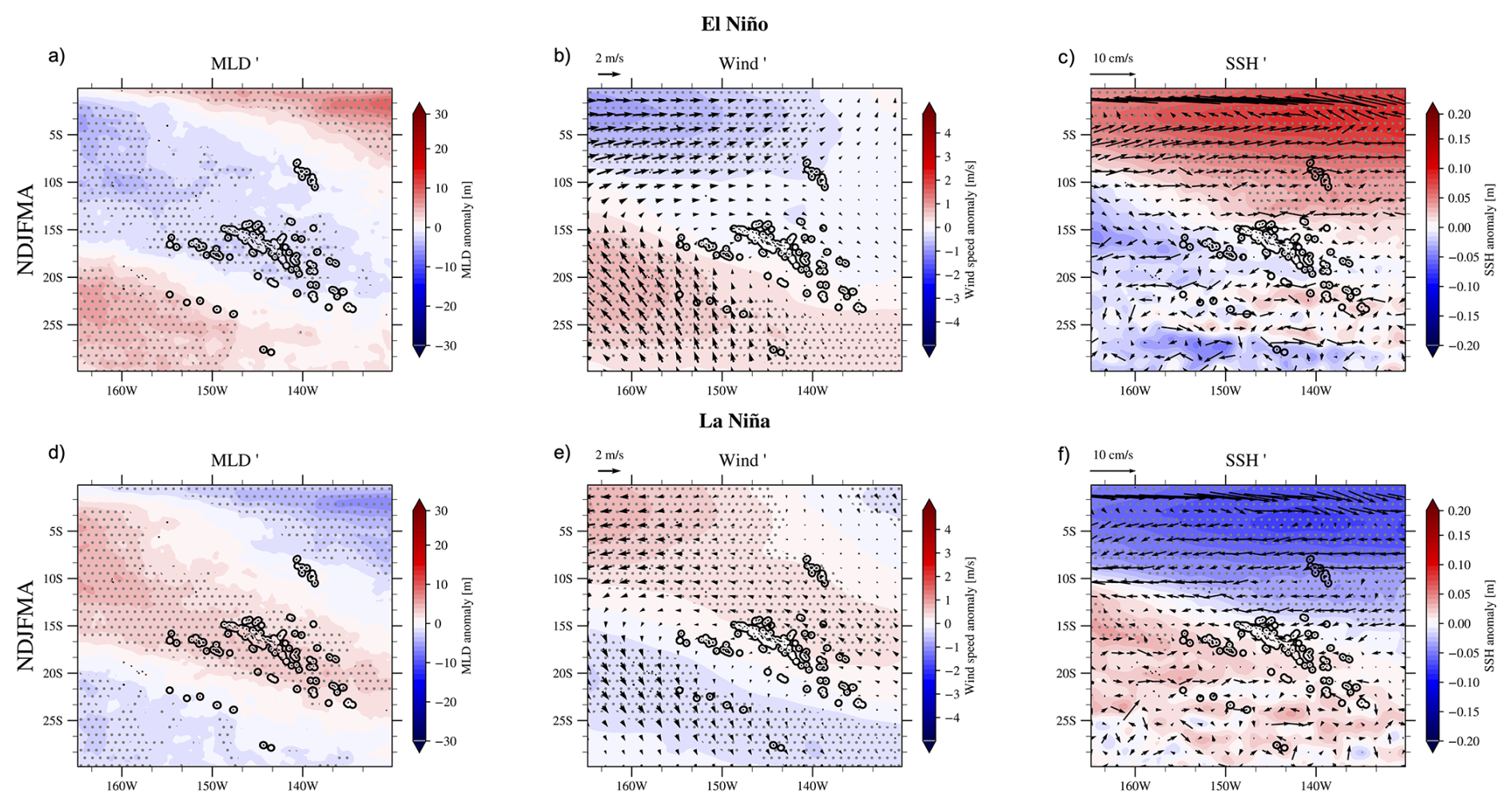
Figure 10 Austral summer El Niño and La Niña composites of the MLD (a, d), 10 m-wind speed and direction (b, e), SSH and oceanic horizontal currents averaged from the surface to 30 m (c, f) anomalies. Gray dots mark anomalies significant at the 95 % confidence level (two-tailed Student t-test). The effective number of degrees of freedom has been computed as $n\frac{(\mathrm{1}-{\mathit{\rho }}_{\mathrm{1}})}{(\mathrm{1}+{\mathit{\rho }}_{\mathrm{1}})}-\mathrm{1}$ following Bretherton et al. (1999) where ρ₁ is the lag-1 autocorrelation of each field and n is the total number of time steps (number of days here).

5.3 The role of ENSO

The role of ENSO and its diversity in modulating the spatial distribution of MHWs has been highlighted in Sect. 4 (Figs. 3–5). The preceding details on the mechanisms involved during the onset and decay phases of MHWs across FP further help to understand ENSO's influence. EN generates positive SST anomalies over the northeastern half of FP and negative anomalies over the southwestern half, with the opposite pattern observed during LN (Fig. 4). These SST anomalies, depending on their signs, reduce or increase the gap to the MHW threshold depending on the region, thereby creating a favorable or unfavorable background state for MHW development. Figure 10 displays surface wind, mixed layer, SSH and surface currents averaged for EN and LN separately. EN periods are characterized by a significant shoaling of the mixed layer, and reduced wind speeds across most archipelagos, therefore creating a favorable environment for MHWs development (by reducing evaporation, rendering the mixed-layer more sensitive to warming from air/sea fluxes and potentially also reducing the efficiency of vertical processes – upwelling, mixing, entrainment – in cooling the mixed layer) over most regions except around Austral Islands (Fig. 10a and b). In addition to that, eastward current anomalies to the north bring warmer waters from the west and induce deeper thermocline over the northeastern part. Conversely, LN periods are associated with a deeper mixed layer over most regions, limiting the MHWs' development. Furthermore, LN events are associated with a deeper (shallower) thermocline to the southwest (northeast) and a shallower mixed layer and weaker winds over the Austral Islands and their southwestern margins due to the anomalous northwesterly winds (Fig. 10e). This clearly aligns with the spatial modulation of MHWs by ENSO revealed in Fig. 3. ENSO thus acts as a large-scale forcing over FP, promoting the development of MHWs in some regions while inhibiting them in others. Although a full characterization of how different ENSO flavors modulate MHW mechanisms is beyond the scope of this study, Figs. 4 and 5 suggest that both the spatial pattern and the amplitude of wind, mixed-layer and currents interannual anomalies likely depend on the ENSO flavor, consistent with flavor-dependent wind and precipitation anomalies (Pagli et al., 2025a). This can explain the differences observed in MHW properties and occurrences during the different EN and LN flavors (Figs. 4, 5, and S10).

6 Discussion

Our results regarding the classification of MHWs into different types (Q, HADV, RES) over the South Central Pacific (Fig. 6) align with previous global modeling studies investigating dominant MHW mechanisms with mesoscale-resolving models (Marin et al., 2022; Bian et al., 2023, 2024) when looking at the spatial repartition of Q-MHWs and HADV-MHWs dominated-regions. It is interesting to note that the conclusions obtained here about the mechanisms of all MHWs in FP correspond to that obtained by looking at the most extreme events over the region in the global-scale study of Marin et al. (2022) (their Figs. 3 and 4). RES-MHWs, which are predominant in the equatorial region north of 2° S, have been mainly attributed to anomalous vertical mixing processes that warm the mixed layer during the onset and decay phases (Bian et al., 2023). Further south, over FP, the residual contributions observed during onset and decay in our analysis (Figs. A1 and A2) have not been explored in detail in this study because the amplitude of the data assimilation increments is unknown. Nevertheless, as stated in our study this residual may partly reflect the effect of weakened winds during MHW onset and decay (Fig. 9) that are favored by EN (in the northeast) and LN (in the southwest), which can reduce vertical heat transfer through diffusion and local mixing (Vogt et al., 2022). It has also been shown that mesoscale eddies can inhibit the vertical mixing driven by internal waves over the region, limiting subsurface cooling and thereby promoting the development of extreme subsurface temperatures (Wyatt et al., 2023). Tides – and therefore internal tides – are not explicitly represented in GLORYS, and FP is a major internal-tide generation region (Zaron, 2019). The substantial number of RES-MHWs detected over FP (Fig. 6c and g) therefore highlights the need for regional modeling that resolves tidal processes.

One limitation of our study is its focus on surface temperatures, whereas extreme temperatures can also occur throughout the water column with severe impacts on ecosystems (Wyatt et al., 2023) – either synchronously with the surface, more intense, less intense, or even entirely decoupled from surface extremes (Zhang et al., 2023). The mechanisms driving these subsurface extremes may differ from those at the surface revealed in this work, due to the vertical structure of ocean currents in the region and the progressive attenuation of air–sea flux influences with depth. Our analysis gives confidence in GLORYS, to study vertical extent of MHW. Lal et al. (2025) showed that surface MHWs in the extreme western part of FP are generally confined to the seasonal mixed layer north of 20° S, but extend deeper south of this latitude, providing an indication of what might be expected for the vertical extent of MHWs detected over FP in this study.

We showed that ENSO provided favorable or unfavorable background conditions for MHW development during the warm season and to a lesser extent over the austral winter, depending on the region within FP and the ENSO phase. However, except in the extreme northern regions, including the Marquesas during extreme EPEN and strong MEN events – where the surface ocean remains in a persistent MHW state throughout the whole warm season – the actual triggers of the mechanisms creating MHW onset (extreme LHF and SW anomalies) remain to be fully understood. Intra-seasonal processes such as the Madden–Julian Oscillation (MJO), equatorial wave activity, and/or stochastic weather/oceanic events (Tropical Cyclones, prolonged periods of high/weak surface winds, prolonged precipitation/clear sky periods, SPCZ intra-seasonal variability, oceanic eddies) may initiate or terminate MHWs. In this context, ENSO primarily modulated the background state, influencing how these intra-seasonal triggers affect MHW development and persistence (MJO-ENSO compound events as an example, Dutheil et al., 2024). Further work is needed to understand how ENSO and these higher frequency variations interact together.

Our work builds on ongoing efforts to understand the characteristics and mechanisms of MHWs across South Pacific countries (Holbrook et al., 2022; Dutheil et al., 2024; Lal et al., 2025). MHWs display distinct features between the western and central South Pacific, underscoring the need for such regional analyses. Even within the FP region, while we present results at the archipelago scale, notable variability was found within the Tuamotu archipelago itself, which spans from about 10° N to 23° S (Fig. 3e).

Many of the FP islands (except in the Marquesas) are fringed by reefs that enclose lagoons, which most of the time represent a key economic resource for local communities. MHWs can have devastating impacts on such ecosystems (Glynn, 1984; Mumby et al., 2001b; Andréfouët et al., 2015; Andréfouët and Adjeroud, 2019; Hédouin et al., 2020). These lagoons exhibit diverse geomorphological characteristics, such as differences in size and degree of openness to the open ocean, making it challenging to assess how large-scale oceanic MHWs propagate into these more sheltered environments. To achieve this at the atoll and lagoon scale, this requires validating high-resolution satellite SST products against in-situ observations (e.g., ReefTemp; Van Wynsberge et al., 2017; Le Gendre et al., 2024), alongside a detailed understanding of lagoon hydrodynamics (Bruyère et al., 2023). Additionally, the development of hydrodynamical or statistical models that relate lagoon interior surface temperatures to oceanic temperatures and ocean–meteorological conditions could help compensate for the current lack of high-resolution SST data (Van Wynsberge et al., 2017, 2024).

In Fig. 5 we related ENSO flavors to DHW, the NOAA metric used to monitor coral bleaching globally. NOAA's historical alert levels are: 0–4 (possible bleaching), 4–8 (reef-wide bleaching risk), and > 8 (reef-wide bleaching with potential mortality). In our record, the 8 threshold is rarely reached in the Society and Tuamotu – even in 2015/16 (Figs. 5 and S11), when widespread bleaching was documented (Hédouin et al., 2020). This underscores known limitations of the standard DHW formulation, which can underpredict bleaching and overlooks regional sensitivities. It has been shown that tuning the hotspot definition, accumulation window, and/or bleaching threshold improves coral bleaching forecast skill (e.g. Lachs et al., 2021; Whitaker and DeCarlo, 2024) but that these adjustments often become region- or location-specific, rendering generalization difficult. Accordingly, Fig. 5 quantitative results should not be read as direct indicator of coral bleaching; rather, it shows how ENSO modulates cumulative heat stress across FP's archipelagos. Bleaching occurrence is also modulated by other environmental factors than heat stress – e.g., UV-exposition, the shortwave radiation reaching colonies at depth, salinity, water depth, nutrient supply, and local hydrodynamics (DeCarlo et al., 2020; Gonzalez-Espinosa and Donner, 2021). As an example, over FP, increased cloud cover has been suspected to spare Society Islands from massive coral bleaching in the extreme EPEN 1997/98 event (Mumby et al., 2001a).

While the OISST dataset has been shown to be well-suited for the analysis carried out in this study Gupta and Sil, 2024), differences between SST products can be significant for some commonly used MHW metrics (Chevillard et al., 2025) and this should be kept in mind. For analyzing ENSO modulation, products generally yield consistent patterns (here OISST and GLORYS are coherent). However, at the archipelago scale, quantitative metrics can differ between products (Fig. S7).

Our results provide crucial insights into the mechanisms driving MHWs over FP and their link with ENSO, which are essential for improving seasonal-to-interannual forecasts of these extreme events. The forecasting skill of MHWs varies significantly depending on season, region, and lead time (de Boisséson and Balmaseda, 2024; Cohen et al., 2025; Jacox et al., 2022). In particular, there is a strong ENSO imprint on the predictability of these events. Over the northeastern region of FP, MHWs appear much more predictable than in southern regions, with minimal forecast skill in the central areas where MHWs are primarily controlled by air–sea fluxes (Fig. 6). In the southwestern part of FP, MHW forecast skill is also weak, likely due to the dominant influence of horizontal advection (HADV) and mesoscale circulation features during the MHW onset and decay. These findings point to the need for higher-resolution models, along with an expanded network of ocean observations, to improve verification of the models and forecasting capabilities in this region.

Across the entire FP region, both the number of MHW days and event durations have increased over time (Fig. S20). However, maximum intensity has increased only in the southwestern half of the country – including the Society Archipelago, southern Tuamotu, Gambier, and Austral Islands – while the northern Tuamotu and Marquesas have experienced a decrease in maximum MHW intensity over time (Fig. S20b). The spatial pattern of this trend closely mirrors that of the long-term SST trend across the region (see Fig. S1). The underlying cause of this cooling trend in the northeast which extends more broadly in the eastern tropical Pacific remains to be clarified – whether it reflects the influence of global warming, natural tropical Pacific decadal variability, or more likely a combination of both (Watanabe et al., 2024). Therefore, the observed cooling trend in MHWs intensity over the northeastern region needs to be interpreted carefully.

7 Conclusion

The present study provides a comprehensive assessment of MHWs in the south central Pacific across FP, characterizing their spatial and seasonal variability, mechanisms, and modulation by ENSO and its various flavors. MHWs were analyzed using OISST data for the 1981–2024 period, as well as with the GLORYS reanalysis for 1993–2024. GLORYS agreement with OISST gave us confidence in the ability of the reanalysis to study MHW mechanisms over 1993–2020. Hence, by examining the mixed layer heat budget during MHWs in GLORYS, we were able to determine the main mechanisms at work during MHW intensification and decay phases.

We showed that MHW occurrence, intensity, and duration vary significantly between archipelagos and seasons. The Marquesas and Austral Islands experienced the highest number of MHW days during the warm season, as well as the most intense and long-lasting events. In contrast, the Society, Tuamotu, and Gambier Islands tend to experience MHWs of lower intensity and duration, particularly during the cold season. Cumulative intensity and duration extremes also varied spatially, reflecting region-specific mechanisms.

Our results highlight the dominant role of air–sea fluxes in driving MHWs in the central regions (Society–Tuamotu–Gambier), while oceanic advection is the key mechanism generating MHWs in the Marquesas and equatorward zones up to 2° S where vertical processes dominate. In the Austral Islands and poleward zones, both air–sea fluxes and horizontal advection contribute comparably. During the cold season, the role of horizontal advection becomes more prominent across FP, while the impact of surface fluxes is dampened by a deeper seasonal mixed layer. Generally, most of MHWs decay is driven by air–sea fluxes.

We also demonstrated that ENSO exerts a strong and spatially structured modulation on MHWs in FP. EN favors MHW development in the northeastern region (Marquesas–northern Tuamotu), while LN promotes MHWs in the southwest (Austral Islands). These effects are linked to seasonally persistent changes in SST, surface wind speed, MLD, and oceanic horizontal advection patterns.

This work provides new insights into the processes controlling MHWs across FP and their connection to large-scale climate variability. It also offers a framework for understanding how future changes in ENSO behavior and ocean–atmosphere coupling might influence the frequency and severity of MHWs over the region.

Appendix A

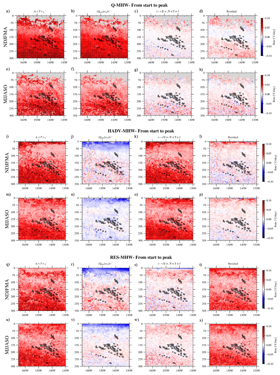
Figure A1 Composites across all events at each grid point of the different term of the heat budget analysis Eq. (2) averaged from start to peak for each MHW type and for each season separately. The first column corresponds to the mixed-layer temperature tendency term, the second one corresponds to air/sea flux heat budget term, the third one corresponds to the horizontal heat advection term and the fourth one corresponds to the residual term. They are all expressed in °C d⁻¹. Panels (a)–(d) and (e)–(h) show composites of Q-MHWs during austral summer and winter, respectively. Panels (i)–(l) and (m)–(p) show composites of HADV-MHWs for summer and winter, respectively. Panels (q)–(t) and (u)–(x) present composites of RES-MHWs in austral summer and winter, respectively.

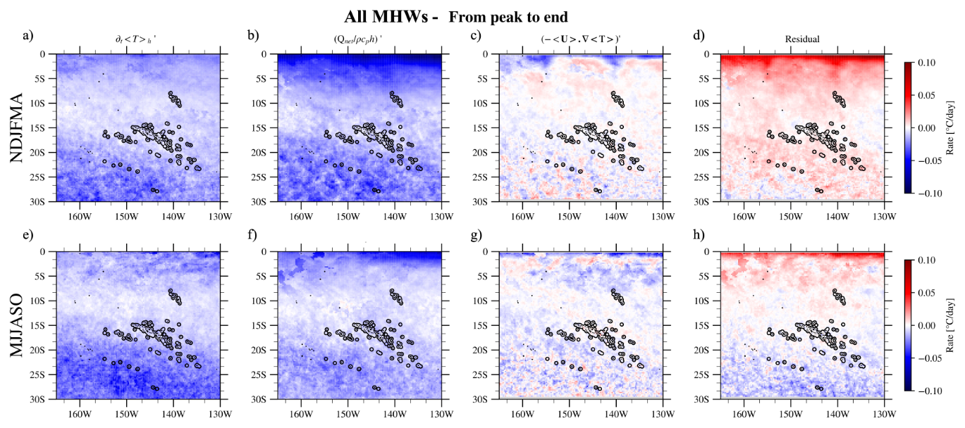
Figure A2 Composites across all events at each grid point of the different term of the heat budget analysis Eq. (2) averaged from peak to end for all MHWs and for each season separately. The first column corresponds to the mixed-layer temperature tendency term, the second one corresponds to air/sea flux heat budget term, the third one corresponds to the horizontal heat advection term and the fourth one corresponds to the residual term. They are all expressed in °C d⁻¹. Panels (a)–(d) and (e)–(h) show the composite over MHWs in austral summer and winter, respectively.