Sensitivity of marine heatwaves metrics to SST products, focusing on the Tropical Pacific

Marine heatwaves (MHWs) are increasingly studied in climate sciences for their ecological impacts, for which accurate real-time bulletins and forecasts are essential. Yet, methodological choices in their detection affect metric estimates, underlining the need to better assess these sensitivities. This study provides a thorough assessment of the impact of sea surface temperature (SST) product choice on MHW statistics, focusing on the tropical Pacific. MHW detection was performed on six daily gridded SST datasets: four widely used blended satellite observational products, one ocean reanalysis, and a multi-dataset ensemble mean computed from the four observational products. Sensitivity to SST products was evaluated for six MHW metrics (MHW days per year, number of events per year, duration, maximum intensity, cumulative intensity and onset rate) and for the degree heating weeks (DHW), a widely used index for coral bleaching risk. Inter-product comparisons revealed a significant dispersion among MHW metric estimates. The reanalysis GLORYS12v1 detected fewer, longer and less intense MHWs while OISST detected more MHWs of shorter duration and higher intensity. likely related to the respectively weak and strong high-frequency SST variability (periods shorter than 2 weeks) of the two products. The sensitivity analysis showed that the onset rate was the most sensitive metric to SST product choice and the maximum intensity the most robust one. Metrics uncertainties were quantified inside seven regions of the basin and were largest in the western Pacific Warm Pool. Co-occurrence analyses of MHWs revealed that, over the basin, 10 % to 80 % of MHW days were detected simultaneously by all products, with the western Pacific Warm Pool showing the lowest agreement (10 %–40 %). Filtering MHWs by size also revealed that the detection of large-scale MHWs ($>\mathrm{5}\mathit{°}\text{lon}\times \mathrm{5}\mathit{°}\text{lat}$) was more consistent across products than smaller-scale ones. Finally, over the studied period, inter-product differences tended to decrease with time. The DHW also revealed to be sensitive to SST products, with inter-product differences on DHW annual maximum reaching more than 1 °C weeks and percentages of bleaching alert days (DHW≥4 °C weeks) in common across products reaching 70 % at most across much of the basin. These findings contribute to a better understanding of how SST product choice affects the characterization of MHWs and DHW, and their associated uncertainties.

1 Introduction

Between April 2023 and July 2024, global ocean surface temperatures reached their highest level ever registered (Terhaar et al., 2025). These extremes observed in global mean sea surface temperatures (SST), partly related to an El Niño event, would not have been reached without the acceleration of ocean warming over the last decades (Merchant et al., 2025). They manifest locally as “marine heatwaves” (MHWs), a term first introduced by Pearce et al. (2011). Hobday et al. (2016) further formalized the definition of a MHW as an episode of temperatures above a climatological threshold for at least five consecutive days, characterized by its duration, intensity, rate of evolution and spatial extent. Due to their significant ecological and biological impacts (Capotondi et al., 2024), MHWs have become a hot topic in ocean science, more so as climate models predict significant increases in their frequency, intensity and duration due to global warming (Frölicher et al., 2018; Oliver et al., 2019).

Real-time MHW information and forecasts are of crucial interest to managers and stakeholders as they support marine conservation and fisheries management (Holbrook et al., 2020; Hartog et al., 2023; Hobday et al., 2023; Kajtar et al., 2024; Spillman et al., 2025). Such bulletins must provide accurate information, ideally combined with uncertainty estimates. Explicitly accounting for the methodological choices in MHW detection (Farchadi et al., 2025), and, consequently, quantifying the associated uncertainties, are key to MHW research and to assess their socio-ecological impacts.

MHW detection requires several methodological choices: the choice of the SST product, the definition of the climatological baseline, whether or not to detrend the SST time series, and the definition of the MHW threshold (Farchadi et al., 2025). For better agreement across studies, the scientific community usually agrees on a common methodology (use of 30 year climatology, no detrending and seasonally varying 90th percentile, Hobday et al., 2016), but other options can lead to significantly different results in MHW metrics evaluation potentially leading to different policy responses to MHWs (Capotondi et al., 2024).

While the effects of the climatological baseline choice (Amaya et al., 2023), of detrending (Smith et al., 2025) and of the use of a fixed threshold (Langlais et al., 2017) have been investigated and discussed, the impact of SST product choice on MHW detection statistics remains little explored. This step appears crucial for MHW analysis (Farchadi et al., 2025), yet most MHW studies rely on a single blended SST product, either satellite-only or satellite combined with in situ data, or an ocean reanalysis. A similar issue applies to the degree heating weeks (DHW) computation, a widely-used metric for coral bleaching risk that represents accumulated heat stress which can lead to coral bleaching and mortality (Skirving et al., 2020). This metric is also computed from a single SST product in most coral studies. Yet, SST products differ in their data sources, processing and interpolation methods, and they consequently exhibit differences (Martin et al., 2012; Dash et al., 2012; Okuro et al., 2014).

Several studies have focused on intercomparing satellite-derived SST products, particularly with regard to trends (Menemenlis et al., 2025) or through validations using in-situ observations (Fiedler et al., 2019). Nevertheless, while some studies have shown that MHW characteristics can be biased depending on the chosen SST product (Wang et al., 2024; Lal et al., 2025), the sensitivity of MHW metrics to the choice of SST product has been scarcely investigated, and to our knowledge, has never been quantified at global or basin-wide scales. Marin et al. (2021) identified locations where significant differences between products occur, but for coastal MHWs. For DHW, several studies showed significant differences between datasets in specific areas (for instance, Neo et al., 2023, compared four datasets in the North Western and South Western Australian reefs; Margaritis et al., 2025, compared two datasets in the Caribbean).

Such quantification would help improving the consistency of MHW information, which is crucial in basins like the tropical Pacific where communities heavily rely on marine resources (Holbrook et al., 2022; Lal et al., 2025). In this large zone (almost half of the tropics), MHWs are modulated by El Niño Southern Oscillation (ENSO) (Holbrook et al., 2019; Sen Gupta et al., 2020; Pagli et al., 2025), although other phenomena, such as the Madden Julian Oscillation (MJO) (Madden and Julian, 1971, 1972) and tropical cyclones, can also influence MHW life cycle (Dutheil et al., 2024). There, societies and environments are particularly vulnerable to MHWs (Andréfouët et al., 2015; Smith et al., 2021, 2024), making the tropical Pacific an area of strong interest to MHW research.

The present study consequently provides a quantitative assessment of the sensitivity of MHW metrics to SST product choice, focusing on the tropical Pacific. Six SST datasets are compared: four blended multi-satellite observational products, one ocean model reanalysis product, and an ensemble-mean product computed as the average of the four SST observational products. Six MHW metrics (number of MHW days per year, number of events per year, duration, maximum intensity, cumulative intensity and onset rate) were analyzed to determine which metrics are more robust to SST product choice. In addition, the sensitivity of DHW index to SST products was assessed. A regional approach was also conducted by dividing the tropical Pacific into seven regions and providing spatially averaged uncertainties for MHW metrics and DHW inside these regions, in line with the recommendations of Farchadi et al. (2025) who highlight the importance of accounting for regional variability in MHW studies.

The present study is organized as follows. Section 2 describes the data and methodology. Section 3 first provides a comparison of MHW metrics across SST products revealing the impact of high frequency SST variability on MHW detection. A quantitative assessment of the uncertainty associated with the SST product choice is then conducted for each metric at both basin and regional scales, highlighting the highest sensitivity in the western Pacific Warm Pool. Lastly, similar analysis and evaluation of DHW uncertainties linked to the SST choices is also performed. Finally, the results are discussed in Sect. 4.

2 Data and methodology

2.1 SST products

In this study, four observation-based products, their ensemble-mean, and one ocean model reanalysis were analysed. We used four daily global L4 (Level 4, gap-free, gridded) SST analysis products: the NOAA Advanced very High Resolution Radiometer (AVHRR) Optimum Interpolation (OI) $\mathrm{1}/\mathrm{4}$° daily SST v2.0 Analysis data (hereafter designed as OISST), the ESA C3S global Sea Surface and Sea Ice Temperature Reprocessed product (hereafter designed as C3S), the global ocean OSTIA SST and Sea Ice reprocessed product, and the NOAA Coral Reef Watch (CRW) version 3.1 daily global 5 km SST product known as CoralTemp. These products are among the most commonly used in MHW studies. We also used the ocean reanalysis GLORYS12v1 as: (1) reanalyses are widely used in MHW research to better understand MHW vertical extent and driving mechanisms (Capotondi et al., 2024; Dutheil et al., 2024), (2) this reanalysis is also used for MHW reports/forecasts by Mercator-Ocean for Copernicus Marine Service (https://www.mercator-ocean.eu/ocean-intelligence/ocean-bulletins-and-insights/marine-heatwaves-archive/, last access: 7 March 2025). The GLORYS12v1 reanalysis used here is a $\mathrm{1}/\mathrm{12}$° reanalysis using the NEMO (Nucleus for European Modelling of the Ocean, Madec et al., 2024) ocean model, forced by ECMWF ERA-Interim atmospheric reanalysis (Dee et al., 2011), complemented by ERA5 re-analyses (Hersbach et al., 2020) for recent years (from 1 January 2019). This reanalysis assimilates sea level anomalies (SLA), observed SST (OISST), sea ice concentration and in situ temperature and salinity vertical profiles (Lellouche et al., 2021).

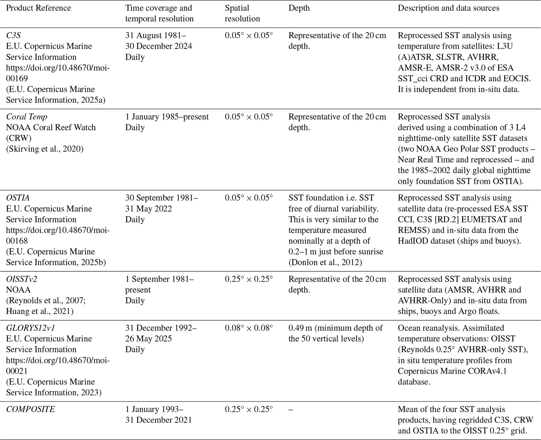
For MHW inter-comparison, C3S, OSTIA, CRW and GLORYS12v1 were regridded on the OISST 0.25° grid using the conservative method “remapcon” from CDO software (Schulzweida, 2023). Finally, a sixth dataset hereafter referred to as “COMPOSITE”, was constructed to evaluate the relevance of a multi-product approach for MHW analysis. More precisely, the daily 0.25° COMPOSITE was computed as the mean of the four SST observation-based products: the three re-gridded C3S, CRW and OSTIA, and the raw OISST. The reanalysis GLORYS12v1 was not included in the COMPOSITE since it differs by definition from observation-based products. MHW detection was thus performed on these six 0.25° daily datasets. A summary of information for these datasets is provided in Table 1.

Table 1 Description of the SST datasets.

2.2 MHW and DHW analyses

2.2.1 Study area

MHW and DHW analyses were performed over the tropical Pacific (30° S–25° N; 125° E–70° W, Fig. 1a) at 0.25° spatial resolution. The latitudinal coverage is not symmetric with respect to the equator, extending further south to include islands of the southern subtropical Pacific, notably French Polynesia (30–0° S; 165–130° W). As MHW characteristics and ocean processes vary within this area (Holbrook et al., 2019, 2022; Lal et al., 2025), the sensitivity analysis was conducted at regional scale for both MHW metrics and DHW. Seven regions were defined based on the Longhurst (2007) provinces which reflect different “eco-regions” functioning with specific physical and biogeochemical ocean properties. As will be shown later, these regions also correspond to areas with distinct MHW characteristics, and represent different physical regimes in the tropical Pacific. Results of the basin-scale sensitivity analysis were thus aggregated within these regions. These regions are drawn in Fig. 1a and named following Longhurst (2007): the North Pacific Subtropical Gyre West (NPSW), North Pacific Tropical Gyre (NPTG), West Pacific Warm Pool (WARM), North Pacific Equatorial Countercurrent (PNEC), Pacific Equatorial Divergence (PEQD), Archipelagic Deep Basins (ARC) and the South Pacific Subtropical Gyre Province (SPSG) (Fig. 1a). Minor adjustments were made to the original WARM province of Longhurst (2007), with a small extension further east at the borders with the PNEC and SPSG, to better capture the coherent dispersion patterns of MHW metrics.

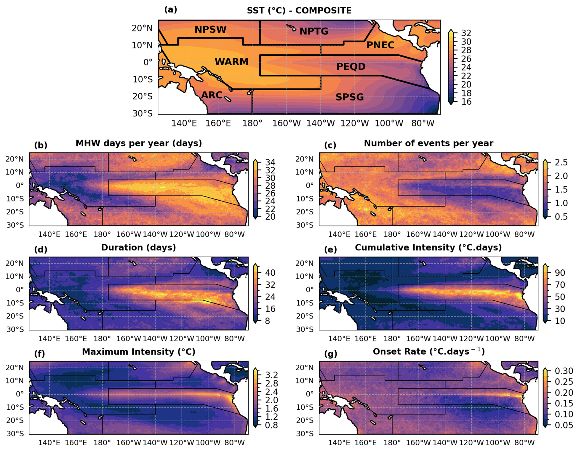
Figure 1 (a) Mean SST (1993–2021) from the COMPOSITE in the tropical Pacific, with the regions of study. (b–g) Ensemble mean of MHW metrics in the tropical Pacific (1993–2021; cf. Sect. 2.3.1), with the limits of the regions defined in (a).

2.2.2 MHW and DHW computation

MHW detection was performed for each pixel of the six datasets presented in Sect. 2.1 on the 0.25° common grid over the tropical Pacific and the period 1993–2021, following the Hobday et al. (2016) method. A MHW event was defined as a period of at least five consecutive days during which SST exceeded the local 90th percentile threshold. Events separated by fewer than two days were considered as a single continuous event. The full study period 1993–2021 also served as the common climatological baseline across the SST products (Table 1, common period to all products). No detrending was applied to the SST time series in order to account for differences in long-term SST trends among products (Menemenlis et al., 2025). The sensitivity analysis was carried out for six MHW metrics: (1) the number of MHW days per year, (2) number of events per year, (3) event duration, (4) maximum intensity, (5) cumulative intensity, and (6) onset rate. The number of MHW days per year and the number of events per year were defined as the total number of days and events over 1993–2021 divided by the 29 years of the analysis period. Maximum and cumulative intensities were expressed relative to climatology, with cumulative intensity calculated as the sum of daily intensities over each event's duration. The onset rate was defined as the rate of temperature increase from the start of a MHW to its maximum intensity (Hobday et al., 2016).

Daily degree-heating weeks (DHW) values were computed following Skirving et al. (2020) for each pixel of the six SST datasets of Sect. 2.1 at 0.25° resolution. First, daily temperature anomalies (HotSpot) were calculated relative to the local Maximum of Monthly Mean (MMM), defined as the maximum of monthly climatological means over 1993–2021. DHW values on a given day were then computed as the sum over the preceding 12 weeks of daily HotSpot anomalies exceeding 1 °C. This accumulated sum was divided by 7 to express DHW in °C weeks. Due to its ecological relevance, we investigated the impact of SST product choice on the yearly maximum DHW values in the tropical Pacific. More precisely, this metric quantifies the maximum accumulated heat during a year that can potentially stress marine organisms such as corals.

2.2.3 Filtering MHWs by size

In order to better understand the origin of inter-product differences in MHW metric estimates, MHWs were filtered by size. The sensitivity analysis was carried out for micro (maximum area $\le \mathrm{5}\mathit{°}\text{lon}\times \mathrm{5}\mathit{°}\text{lat}$) and macro (maximum area $>\mathrm{5}\mathit{°}\text{lon}\times \mathrm{5}\mathit{°}\text{lat}$) events, separately. MHWs spatial extent was characterised as follows: for each day, all pixels where MHWs were detected were assigned a MHW area, defined as the number of contiguous pixels to the studied pixel also experiencing a MHW. These joint pixels are connected along either north-south or west-east directions and were detected thanks to the label function from python package scipy.ndimage (method inspired from Bonino et al., 2023). In a pixel, a MHW was thus associated with a series of areas over its duration. The maximum area reached during the event was associated with each MHW in the evaluated pixel. Events with a maximum area smaller than 25 square degrees (5°×5°) were classified as micro-scale, whereas those with a maximum area exceeding 25 square degrees were defined as macro-scale. The threshold of 25 square degrees was chosen as it filters out MHWs linked to large mesoscale eddies and it is in line with other MHW studies (Lal et al., 2025; Sen Gupta et al., 2020; Sun et al., 2023). The distribution of MHW maximum sizes in the tropical Pacific for all studied products confirmed that this threshold was appropriate for our study (not shown). The 4°×4° threshold was also tested and our results remained almost unchanged, showing that our analysis is robust and not highly dependent on the threshold chosen (not shown).

However, since our area of study is bounded spatially, the spatial extent of MHWs at the northern and southern frontiers of the tropical Pacific should be considered carefully (joint pixels can't extend further south and north, respectively). MHWs spatial extent at these frontiers might actually be larger than it appears in our results.

2.2.4 Filtering MHWs according to El Niño Southern Oscillation

Since ENSO is a dominant driver of MHWs in the tropical Pacific (Holbrook et al., 2019; Sen Gupta et al., 2020; Pagli et al., 2025), the dependence of our results on the ENSO phase was explored. For this purpose, MHWs were divided into three groups: El Niño MHWs, La Niña MHWs, and neutral MHWs. El Niño MHWs were defined as MHWs starting during a month where the Oceanic Niño Index (ONI) was higher than 0.5 and La Niña MHWs were defined as MHWs starting during a month where the ONI was lower than −0.5. The monthly timeseries of the ONI used here are available at: https://psl.noaa.gov/data/timeseries/month/ (last access: 13 January 2026). All other MHWs were classified in the neutral group.

2.3 Sensitivity analysis

2.3.1 Inter-product differences and uncertainty quantification

Inter-product differences in MHW detection were illustrated by maps of mean MHW metrics for each SST product over the tropical Pacific and the time period (1993–2021). For duration, maximum intensity, cumulative intensity and onset rate, each pixel of these maps was defined as the mean value across all MHWs detected between 1993 and 2021 in this pixel. For the number of MHW days per year and the number of events per year, the maps were defined at each pixel as in Sect. 2.2.2.

To better highlight the inter-product differences on MHW metrics, anomalies were also mapped over the tropical Pacific. For each product and metric, the product anomaly at each pixel was defined as the difference between the metric value for that product (as defined above) and the ensemble mean value of the metric over all products except the COMPOSITE (i.e. the mean of five values, hereafter designated as “ensemble mean” metric) (Eq. 1):

$$\begin{array}{}\text{(1)}& \begin{array}{rl}\text{anomaly}({\text{metric}}_i& ,{\text{product}}_j,{\text{pixel}}_k)=\\ & {\text{metric}}_i({\text{product}}_j,{\text{pixel}}_k)\\ & -{\text{ensemble}}_{\text{mean}}({\text{metric}}_i,{\text{pixel}}_k)\end{array}\end{array}$$

where ${\text{ensemble}}_{\text{mean}}({\text{metric}}_i,{\text{pixel}}_k)=\left({\sum }_{j=\mathrm{1}}^{\mathrm{5}}{\text{metric}}_i\right({\text{product}}_j,{\text{pixel}}_k\left)\right)/\mathrm{5}$, with i varying from 1 to 6 and representing the six evaluated metrics, j varying from 1 to 5 and representing the 5 products C3S, CRW, OSTIA, OISST and GLORYS12v1, and k representing the pixel number in the domain. The same maps were produced for the temporal mean of DHW annual maxima (Sect. 2.2.2). Mean metrics and anomalies were computed for the COMPOSITE but the latter was removed from the ensemble-based statistics to avoid counting the observational products twice, since the composite is derived from them.

The sensitivity of each MHW metric to SST product choice was evaluated at each pixel by computing the dispersion of the metric across all SST products excluding the COMPOSITE (hereafter designated as “ensemble dispersion”, Eq. 2).

$$\begin{array}{}\text{(2)}& \begin{array}{rl}\mathit{\sigma }& ={\text{ensemble}}_{\text{dispersion}}({\text{metric}}_i,{\text{pixel}}_k)\\ & =\sqrt{\begin{array}{l}\frac{\mathrm{1}}{\mathrm{5}}{\sum }_{j=\mathrm{1}}^{\mathrm{5}}\left[\right({\text{metric}}_i({\text{product}}_j,{\text{pixel}}_k)\\ -{\text{ensemble}}_{\text{mean}}({\text{metric}}_i,{\text{pixel}}_k){)}^{\mathrm{2}}]\end{array}}\end{array}\end{array}$$

The ensemble dispersion was also computed for DHW. Maps of dispersion over the tropical Pacific were produced for each metric. These values of ensemble dispersion were defined as the “uncertainty” of the metric with respect to SST product choice. In order to quantify and compare metrics sensitivity, the ensemble dispersion at each pixel was in some instances expressed as a percentage by dividing the ensemble dispersion by the ensemble mean value of the metric at that pixel, and then multiplying by 100.

The co-occurrence of MHWs across SST products was also assessed by computing the percentage of common MHW days over the basin. At each pixel, this percentage was defined as the number of days detected simultaneously as a MHW in all products excluding the COMPOSITE divided by the ensemble mean number of total MHW days at that pixel. Similar analysis was conducted for DHW, by computing the percentage of common bleaching alerts of level 1 (days for which DHW≥4 °C weeks) across products.

2.3.2 Temporal evolution

The temporal evolution of MHW metrics sensitivity to SST product choice was evaluated by computing yearly time series of ensemble dispersion for each metric and region. For this purpose, yearly maps of MHW metrics and ensemble dispersion over the tropical Pacific were produced, following the method described in Sect. 2.3.1. The year attribution of a MHW was based on its onset. Then, spatial averages of these yearly values of ensemble dispersion were computed within each region, to yield one annual dispersion value per metric and region. The spatial average of ensemble dispersion values inside a region was computed for a given year if dispersion values could be computed for at least 10 % of the pixels of the region.

The temporal evolution of metrics sensitivity to SST product choice was also assessed by computing yearly time series of inter-product spatial correlation within all regions (hereafter designated as “ensemble spatial correlation”). For each region and year, spatial correlation between pairs of products was quantified using the uncentered statistic of pattern correlation (Barnett and Schlesinger, 1987), which correlates fields without removing the spatial means. The uncentered statistic was used here since IPCC reports argue that it is better suited as it includes the response in the global spatial mean, while the centered statistic is more appropriate for attribution because it better measures the similarity between spatial patterns (IPCC, 2001). The uncentered pattern correlation statistic is defined as:

$$\begin{array}{}\text{(3)}& \begin{array}{rl}\text{PatternCorrelation}({\text{product}}_a& ,{\text{product}}_b)=\\ & {\displaystyle \frac{{\sum }_{k=\mathrm{1}}^n{a}_k{b}_k}{\sqrt{{\sum }_{k=\mathrm{1}}^n{a}_k^{\mathrm{2}}{\sum }_{k=\mathrm{1}}^n{b}_k^{\mathrm{2}}}}}\end{array}\end{array}$$

where n is the pixel number in the region, a and b represent yearly metrics for two SST products inside the region.

The value of pattern correlation was considered significant when the associated p-value (based on student t-test) was less than 0.01 (e.g. 99 % significance). For a given metric, region and year, the pattern correlation was computed for all 10 product pairs (pairs excluding the COMPOSITE), and these 10 values were averaged to give the yearly value of the ensemble spatial correlation in the region studied. The spatial correlation inside a region was computed for a given year if ensemble spatial correlation values could be computed for at least 10 % of the pixels of the region.

3 Results

3.1 MHW characteristics in the tropical Pacific

Ensemble mean MHW metrics over 1993–2021 are shown in Fig. 1 in the tropical Pacific, with patterns reflecting spatial variability associated with ENSO. In the central and eastern Equatorial Pacific (PEQD), El Niño largely drives MHW risk (Holbrook et al., 2019; Capotondi et al., 2022). Although MHW occurrences are relatively low in this area (Fig. 1c), the number of MHW days per year is highest, exceeding 32–34 d (Fig. 1b). Here, MHWs have longer durations as they last between 30 to more than 50 d on average (Fig. 1d), and exhibit the highest maximum intensity (more than 3.5 °C, Fig. 1f) and cumulative intensity (more than 100 °C d, Fig. 1e) (Holbrook et al., 2019; Oliver et al., 2021). The highly intense MHWs observed in a narrow band along the Equator (2° S–2° N) near the South American Coast are also associated with the highest onset rates of the tropical Pacific (more than 0.3°C d⁻¹, Fig. 1g).

In the Northeastern tropical Pacific (NPTG), MHWs occur on more than 30 d yr⁻¹ (Fig. 1b) but the number of events is low (∼1 per year, Fig. 1c). These events are relatively long (30 d, Fig. 1d) and intense (cumulative intensity of 40–50 °C d, Fig. 1e). In contrast, the PNEC experiences one of the highest numbers of events (more than 2.5 per year, Fig. 1c, also observed by Holbrook et al., 2019; Oliver et al., 2021). This area, influenced by the North equatorial countercurrent dynamics, is characterized by short (less than 15 d, Fig. 1d) but intense events, with maximum intensity reaching 2.5 °C (Fig. 1f). These features are likely linked to the high SST variability of the region, which favors strong MHW intensities (Oliver et al., 2021).

In the southwest tropical Pacific, MHW occurrence is modulated by La Niña conditions (Sen Gupta et al., 2020; Lal et al., 2025). In the ARC, mesoscale eddies close to the eastern Australian coast (Bian et al., 2023; Chapman et al., 2025) along with downwelling Rossby waves and downwelling-favourable winds also favor MHW development (Misra et al., 2021; Li et al., 2023; Lal et al., 2025). In this region, MHWs are relatively frequent (more than 2 events per year, Fig. 1c) but short (less than 15 d, Fig. 1d, Holbrook et al., 2019). Both the number of MHW days and the maximum intensities are close to the tropical Pacific average (around 25 d and 1.5 °C, respectively, Fig. 1b and f). Similar MHW characteristics are observed in the western SPSG and in NPSW. The Northeastern part of the SPSG close to the PEQD is rather influenced by ENSO, with fewer MHWs of longer duration and lower onset rate. The shortest MHWs (less than 10 d, Fig. 1d) are observed in the WARM region. Here, the number of MHW days per year, as well as the cumulative and maximum intensities reach their lowest levels in the tropical Pacific (∼15 d yr⁻¹, <10 °C d and 1 °C, respectively). Nevertheless, this region records a high number of events with more than 2.5 events per year close to the Papua New Guinea and eastern Indonesian coasts (Fig. 1c, also observed in Holbrook et al., 2019; Oliver et al., 2021).

3.2 Inter-product comparison and ranking

The MHW analysis performed over the six SST datasets reveals significant differences across products, as illustrated by the MHW days per year computed for each product (Fig. 2a–f). The associated maps of anomalies (Fig. 2g–l; Sect. 2.3.1) allow us to more easily identify potential outliers. Figures S1–S5 in the Supplement extend the inter-product comparison to the other metrics.

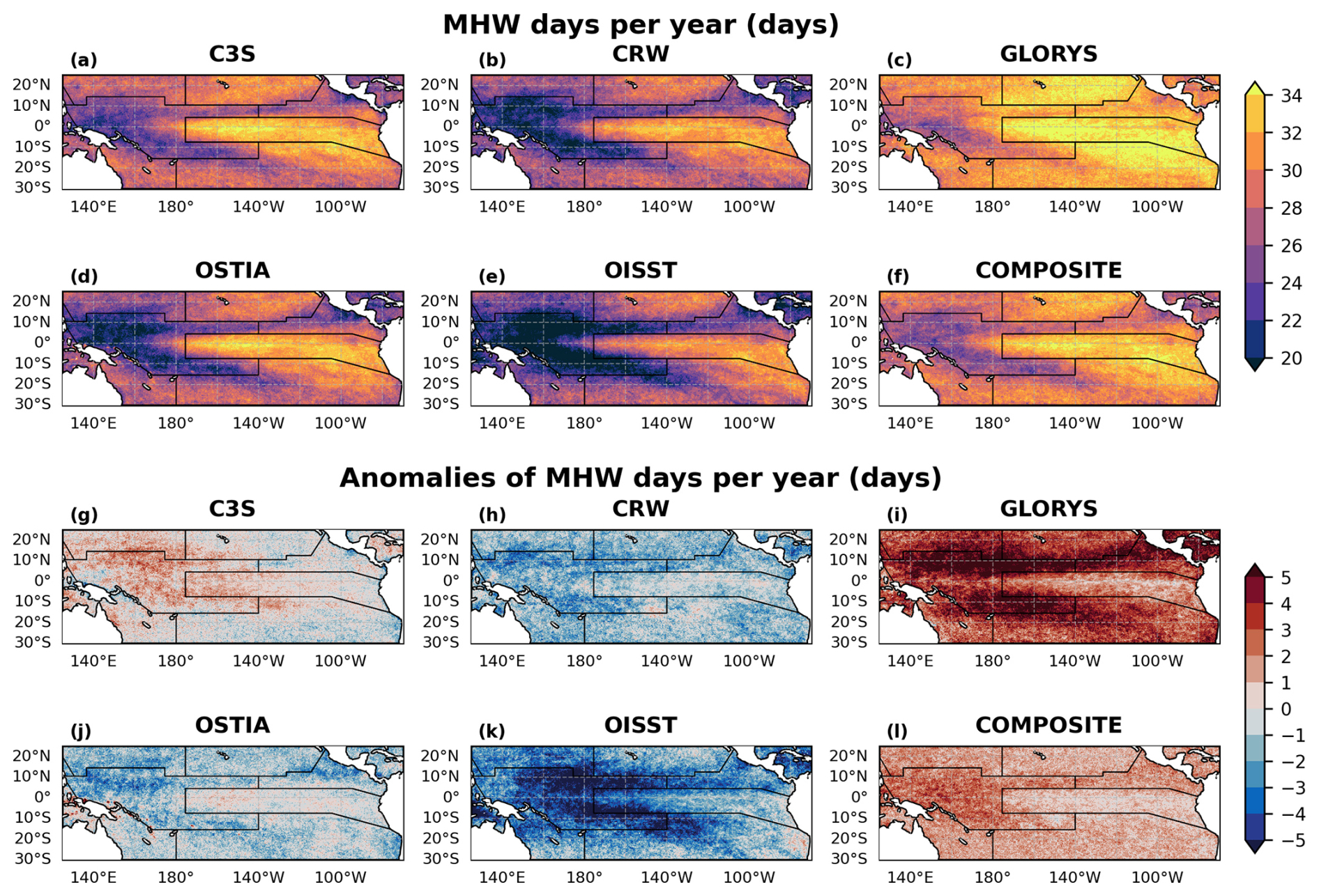
Figure 2 (a–f) Number of MHW days per year over the period 1993–2021 for the six SST products. (g–l) Anomalies of MHW days per year for each product relative to the ensemble mean (Sect. 2.3.1). Black lines indicate regions' limits.

If the main spatial patterns of mean MHW metrics described in Sect. 3.1 are common between all products, Figs. 2 and S1–S5 highlight that values can differ by almost a factor of two between products. For the MHW days per year (Fig. 2a–f), the largest differences are observed in the WARM region, with GLORYS12v1 detecting 30 MHW days per year while OISST detects around 15 d yr⁻¹. Anomalies relative to the ensemble mean range approximately between ±5 d yr⁻¹ inside the tropical Pacific, with some areas showing even larger anomalies (Fig. 2g–l). The strongest positive (negative) anomalies are observed for GLORYS12v1 (OISST). GLORYS12v1 systematically detects more MHW days than the other products, and OISST less MHW days. C3S and OSTIA show smaller anomalies for this metric. For all products, anomalies are closer to zero in the PEQD, a region of strong influence of ENSO where the longest MHWs are observed (Sect. 3.1).

For the other metrics, anomalies generally remain within ±0.5 events per year, ±10 d for MHW duration, ±0.25 °C for maximum intensity, ±15 °C d for cumulative intensity and ±0.15°C d⁻¹ for onset rate over the tropical Pacific (Figs. S1–S5). As for the MHW days per year, anomalies for the other metrics reveal that GLORYS12v1 and OISST show the largest anomalies, whereas C3S, CRW and OSTIA are closer to the ensemble mean – except near Papua New Guinea and eastern Indonesia where OSTIA shows strong positive anomalies in event frequency and onset rate. Unlike the number of MHW days per year, anomalies for other metrics vary substantially in space, and can be either positive or negative within the tropical Pacific for the same product (especially for the number of events per year).

To summarize inter-product differences, the average of MHW metrics for all events detected in the whole domain over 1993–2021 were computed for each product. For a given metric, the minima and maxima across products of these average values were defined so that values on Fig. 3 represent the average value of the given product minus the minimum across products, divided by the difference between maximum and minimum. This normalization standardizes the results between 0 (product ranking last) and 1 (product ranking first) allowing an easier comparison between products. The distance to the center also gives the information on whether the averaged values of some products are closer to others and if some products behave differently. In the study area, OISST ranks first for maximum intensity, onset rate, and the number of events detected (Fig. 3). By “ranking”, we only mean to compare products but not to determine if one performs better than another. Conversely, OISST shows the lowest ranking for the number of MHW days, duration and cumulative intensity (Fig. 3). The opposite pattern is observed for GLORYS12v1 reanalysis which shows the highest ranking for duration, cumulative intensity and the number of MHW days detected, while it ranks last for MHW maximum intensity and onset rate. The COMPOSITE product tends to show a similar radar shape as of GLORYS12v1 (Fig. 3). OISST and GLORYS12v1 also stand out in this study, consistently occupying either the lowest or highest ranks across MHW metric estimates even if their variable ranking differs in a complementary manner. By contrast, C3S shows a more “balanced” radar chart, with no clear overestimation or underestimation compared to other products. These findings are consistent with the anomaly analysis presented in Figs. 2 and S1–S5.

Figure 3 The radar chart is a comparison of all product metrics. The average of MHW metrics are computed for all events detected in the tropical Pacific over 1993–2021 for each product, and normalized by the product that reaches the maximum metric so that all values of the radar chart vary between 0 and 1 (plotted along the radial axes).

The comparison of MHW metrics between products thus highlighted significant differences which vary spatially and between metrics. In the next section, the robustness of the different metrics regarding SST choices is evaluated by quantifying the uncertainty linked to the SST product choice for each metric at both tropical Pacific and regional scales.

3.3 Uncertainty in MHW metrics due to the SST product choice

3.3.1 Basin-scale overview and regional quantification

The MHW co-occurrence analysis (Sect. 2.3.1) reveals that over the basin, between 10 % and 80 % of MHW days are detected simultaneously by C3S, CRW, OSTIA, OISST and GLORYS12v1 (Fig. 4a). Excluding the PEQD region, where percentages reach their maximum ranging between 60 % and 80 %, MHW days in common do not exceed 50 % over the tropical Pacific and even drop below 20 % in a large part of the basin, in the WARM and PNEC regions. The spatial patterns of common MHW days match well with precipitation contours in the basin (Fig. 4a), with highest common days in areas of lowest precipitation in general, an aspect further discussed in Sect. 4.2.

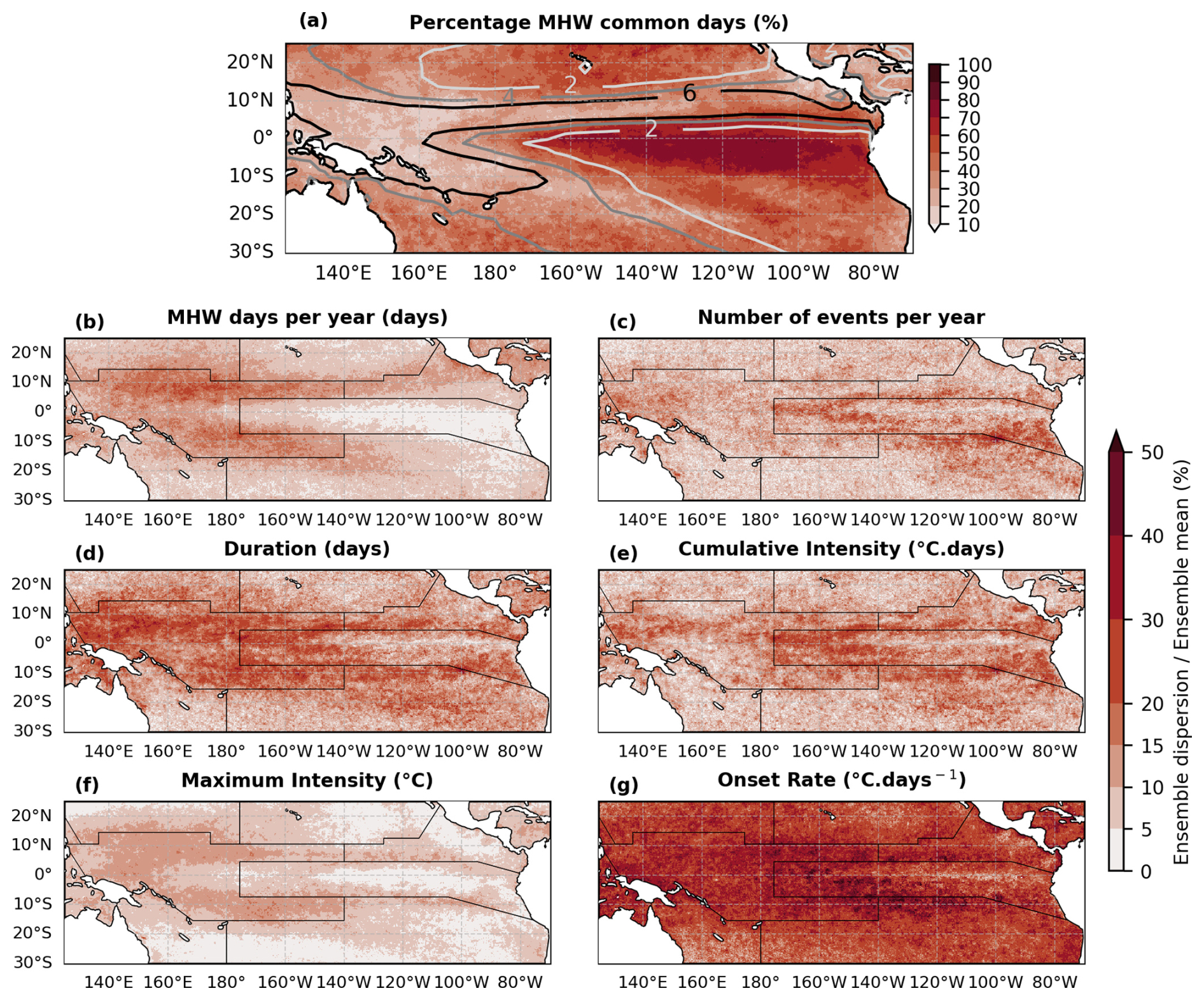
Figure 4 (a) Percentage of MHW days detected simultaneously by C3S, CRW, OSTIA, OISST and GLORYS12v1 (Sect. 2.3.1), with mean 1993–2021 ERA5 precipitation contours overlaid (in mm d⁻¹). (b–g) Normalized ensemble dispersion for each MHW metric (value in %, Sect. 2.3.1). Black lines indicate regions' limits.

The ensemble dispersion normalized by the ensemble mean for each MHW metric (Fig. 4b–g, Sect. 2.3.1) highlights that the onset rate exhibits the largest normalised dispersion across products. Dispersion for this metric exceeds 30 % across much of the tropical Pacific, reaching values above 50 % in the southeastern part of the basin (around 10° S–130 W, Fig. 4g), where onset rates are small (Fig. 1g). MHW duration also exhibits high sensitivity to the choice of SST product, with normalized dispersion ranging between 20 % and 30 % over the basin, closely followed by the cumulative intensity and the number of events per year (Fig. 4c–e). The MHW days per year and the maximum intensity show the lowest dispersion, with values ranging between less than 5 % in the PEQD and 20 % in the WARM for the maximum intensity (30 % for the total MHW days) (Fig. 4b and f).

The high ensemble dispersion values observed in the WARM region across all metrics (Fig. 4b–g) is consistent with the small fraction of MHW days detected simultaneously by C3S, CRW, OSTIA, OISST and GLORYS12v1 in this area (between 10 % and 20 %, Fig. 4a). The spatial patterns of common MHW days also show good correspondence with dispersion patterns of the total MHW days per year and maximum intensity (Fig. 4b and f), with high dispersion coinciding with a low percentage of common days, and vice versa.

The spatial variability of the previous results supports the need of a regional approach in our sensitivity analysis. Consequently, spatial boxplots of dispersion values within each region are represented in Fig. 5. Across regions, the dispersion distributions for each metric differ significantly (Mann–Whitney test, p<0.05). The spatial average of dispersion values within each region is detailed in Fig. 5, providing the uncertainties for each metric and region.

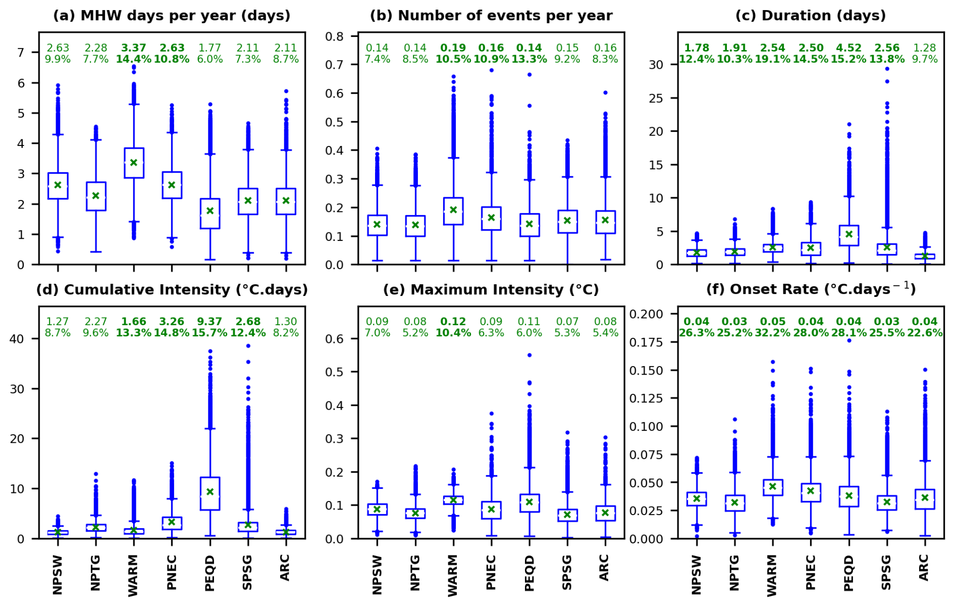
Figure 5 Spatial boxplots of the ensemble dispersion values from Fig. 4b–g for each region. Boxes contain 50 % of the values (limits are the first quartile Q1 and third quartile Q3). Whiskers (lines extending from the box) represent the typical range of data; they extend from $\text{Q1}-\mathrm{1.5}\times (\text{Q3}-\text{Q1})$ to $\text{Q3}+\mathrm{1.5}\times (\text{Q3}-\text{Q1})$. The dots outside the whiskers are considered as “outliers”. The mean values (green marker) are indicated at the top of each boxplot (1st number from the top), along with its equivalence in percentage of the ensemble mean in the region (2nd number from the top). Mean dispersions higher than 10 % of the regional mean value are highlighted in bold.

The regional analysis (Fig. 5) confirms the basin-scale findings (Fig. 4): the onset rate and duration metrics are the most sensitive metrics to SST product choice, with uncertainties exceeding 10 % of the regional means in all regions and peaking in the WARM (32.2 % for the onset rate, Fig. 5). Cumulative intensity also shows uncertainties larger than 10 % in all regions except NPSW and ARC. The number of events per year exceeds 10 % uncertainties in three of the seven regions – WARM, PNEC and PEQD (Fig. 5). Finally, the total MHW days per year and maximum intensity are the least impacted metrics with uncertainty lower than 10 % in all regions except WARM (and PNEC for MHW days per year).

Figure 5 also highlights the WARM region as the most sensitive region to SST product choice, since percentages of dispersion are higher than 10 % whatever the metric chosen. It is closely followed by the PNEC, with uncertainties higher than 10 % for all metrics except maximum intensity. Conversely, NPSW and ARC are the regions that exhibit the lowest uncertainties. The PEQD shows some of the lowest dispersion values among all regions for the total MHW days per year and maximum intensity, but for all other metrics dispersion exceeds 10 % of the ensemble mean. Moreover, the PEQD shows important dispersion values for all metrics with outliers two to three times larger than in other regions for the duration and cumulative intensity (reaching 20 d and 35 °C d, respectively, a pattern also observed in SPSG probably due to ENSO induced variability). Outliers distribution is important as it provides further insights on metrics uncertainties. For example, in PEQD, MHWs detected have an uncertainty of ±0.11 °C in maximum intensity with respect to inter-product differences (Fig. 5). However, some dispersion values inside this region can reach more than 0.5 °C (Fig. 5), suggesting that MHW analyses inside PEQD should be interpreted with caution if based on a single dataset (almost 1 °C of uncertainty for some pixels inside this region).

3.3.2 Metrics uncertainty as a function of MHW size

We now examine whether the metrics sensitivity to the SST product depends on the size of the MHWs. We investigated this by filtering MHWs by size (Sect. 2.2.3), and ensemble dispersion was then computed separately for macro and micro-scale events. Spatial patterns of macro ($>\mathrm{5}\mathit{°}\times \mathrm{5}\mathit{°}$) and micro ($\le \mathrm{5}\mathit{°}\times \mathrm{5}\mathit{°}$) events (Fig. 6a–d) show that macro events occur mainly in regions influenced by El Niño (PEQD and Southeastern SPSG) while micro events are mainly concentrated near coastlines and at the southern and northern limits of the study area (in the PNEC, WARM, ARC, but also northern NPSW and in SPSG near the shore). Yet, the spatial extent of MHWs at the northern and southern limits of the area of study should be taken with caution for the reasons explained in Sect. 2.2.3 (their spatial extent is likely underestimated in Fig. 6).

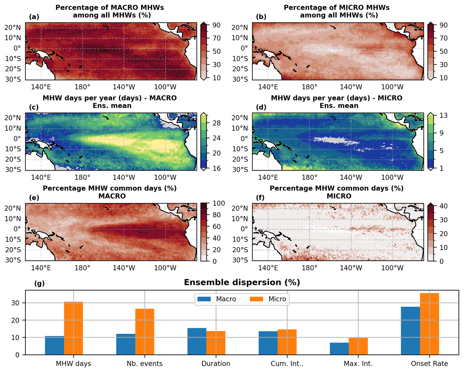
Figure 6 (a) Percentage of macro-scale MHWs among all events detected over 1993–2021 (i.e. ensemble mean of the total number of macro events divided by the ensemble mean of the total number of MHWs of all types, multiplied by 100). (b) Same as (a) for micro-scale MHWs. (c) Ensemble mean of total MHW days per year for macro scale events. (d) Same as (c) for micro-scale MHWs. (e) Percentage of MHW days detected simultaneaously by C3S, CRW, OSTIA, OISST and GLORYS12v1 (Sect. 2.3.1) over 1993–2021 for macro scale events. (f) Same as (e) for micro-scale MHWs. (g) Spatial average over the tropical Pacific of dispersion values for each metric for macro-scale MHWs (blue bars) and micro-scale MHWs (orange bars).

Very few micro-scale MHW days are detected simultaneously by C3S, CRW, OSTIA, OISST and GLORYS12v1 (Fig. 6f): percentages of MHW common days range between 40 % in areas where micro-scale events are numerous and less than 5 % where they are fewer. In contrast, percentages of MHW days in common for macro scale events range between 20 % in the WARM (where they are fewer) and 80 % in the PEQD (Fig. 6e). Differentiating macro and micro-scale events highlights that dispersion is generally lower for macro-scale events (Fig. 6g). This is particularly striking for the total MHW days per year and number of events per year, for which ensemble dispersion decreases by more than two between micro- and macro-scale events when considering spatial averages over the basin. Dispersion for cumulative intensity, maximum intensity and onset rate remains slightly lower for macro-scale events compared to micro-scale events, but is slightly higher for duration.

3.3.3 Temporal variability of the dispersion

Having quantified inter-product differences, we investigated their temporal evolution to assess both long-term trends and the influence of ENSO events on their temporal variability. The yearly time series of MHW metrics averaged over the tropical Pacific for each product highlight the inter-annual variability of inter-product differences (black line Fig. 7), which varies between metrics. Over the basin, differences between products are rather stable through years for the maximum intensity and onset rate while they increase for years marked by strong El Niño events (1997–1998, 2015–2016) for the other metrics (Fig. 7).

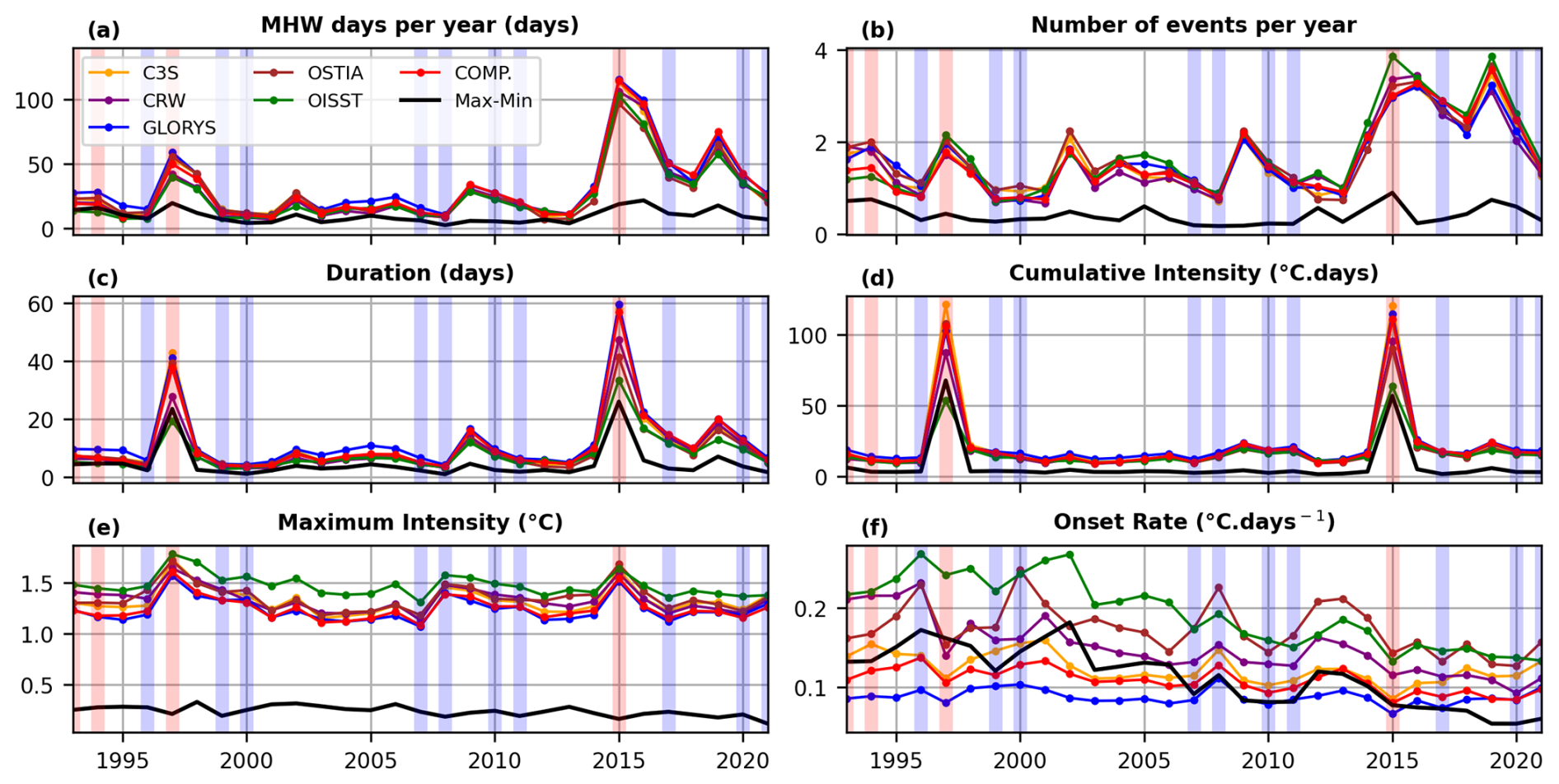
Figure 7 (a–f) Yearly time series of MHW metrics averaged over the tropical Pacific for each product. Inside each panel, the black line represents the largest inter-product difference value for each year (maximum−minimum). The red and blue backgrounds indicate years of strong El Niño and La Niña, respectively, according to the ONI index.

As Fig. 7 reveals a strong influence of ENSO events on MHW metrics, MHW mean metrics and ensemble dispersion were computed for El Niño MHWs, La Niña MHWs and neutral MHWs as defined in Sect. 2.2.4, in the seven regions studied (Fig. 8). Our results being similar between MHW days per year and number of events per year as well as between duration and cumulative intensity, only four metrics (MHW days per year, duration, maximum intensity and onset rate) were illustrated in Fig. 8 to make it more readable. Regional maps of MHW mean metrics for the three groups are also shown in Fig. S6 in the Supplement to better understand Fig. 8. Let's note that the method presented here to classify MHWs should be regarded as a first step and does not account for the substantial diversity among ENSO events. In particular, Eastern Pacific and Central Pacific events (Capotondi et al., 2020) can exert different influences on MHW characteristics (Gregory et al., 2024; Pagli et al., 2025). Figure 8a–d highlights that the PNEC and PEQD are highly influenced by El Niño events while the NPSW and ARC are influenced by La Niña events (in these regions, most MHW days per year are attributed to El Niño and La Niña, respectively). Spatial means of ensemble dispersion inside the regions (Fig. 8e–h) highlight that El Niño leads to lower inter-products dispersion in the regions where it has most influence, while it is not the case for La Niña. The decrease in dispersion in regions influenced by El Niño could be due to the presence of macro scale MHWs during El Niño events, which show lower inter-products dispersion as shown in the results of Sect. 3.3.2.

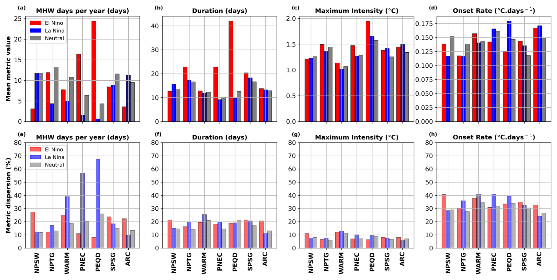
Figure 8 (a–d) Histograms of the spatial means of MHW metrics (ensemble mean) inside the seven regions of study for the MHW days per year (a), duration (b), maximum intensity (c) and onset rate (d) for El Niño MHWs (red), La Niña MHWs (blue) and neutral (gray). (e–h) Histograms of the spatial mean of ensemble dispersion inside the seven regions of study for the MHW days per year (e), duration (f), maximum intensity (g) and onset rate (h) for El Niño MHWs (red), La Niña MHWs (blue) and neutral (gray).

The yearly time series of the ensemble dispersion and spatial correlation within each region (Sect. 2.3.2, Figs. 9 and S7 in the Supplement) provide more insights on the temporal evolution of inter-product differences, and highlight four main points. First, the ensemble dispersion and ensemble spatial correlation values are coherent: metrics showing the lowest dispersion (maximum intensity and MHW days per year) also exhibit the highest ensemble spatial correlation (values ranging between 0.8 and 1), whereas metrics showing the highest dispersion (onset rate) show the lowest ensemble spatial correlation (values ranging between 0.4 and 0.6). The number of events per year, the duration and the cumulative intensity fall in an intermediate range. The WARM region also shows some of the highest and lowest values of dispersion and spatial correlation, respectively, across all metrics.

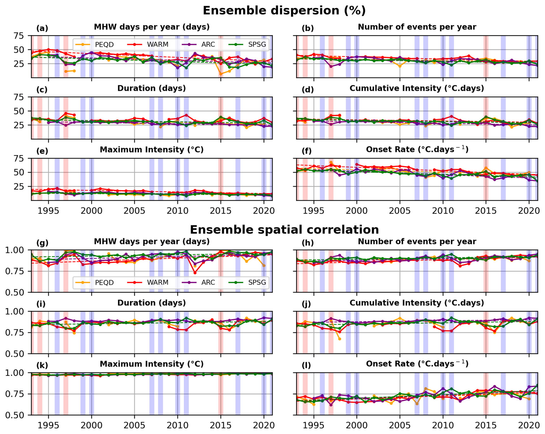
Figure 9 (a–f) Yearly time series of ensemble dispersion (in percentage) for PEQD, WARM, ARC and SPSG. The dashed lines indicate the significant linear trends (p-value<0.05). The red and blue backgrounds indicate years of strong El Niño and La Niña, respectively, according to the ONI. (g–l) Same as (a–d) for the ensemble spatial correlation (Sect. 2.2.3). Time series in the PNEC, NPTG and NPSW are represented in Fig. S7.

Second, yearly ensemble dispersion values are higher than those computed on the mean of metrics as in Fig. 4, suggesting that ensemble dispersion might be underestimated when it is computed on the mean of metrics over a long period rather than on MHW yearly metrics.

Third, the long-term trends suggest a reduction in the inter-product dispersion and an increase in the spatial correlation over the period 1993–2021 for all metrics and regions (Figs. 9 and S7). In all regions, the largest decreases in ensemble dispersion are observed for the total MHW days per year and the onset rate (−6.6 % per decade in WARM and −7.2 % per decade in NPSW, respectively, p-values<0.05) while the lowest ones are observed for the maximum intensity (between −1.1 % per decade and −2.7 % per decade in SPSG and WARM, respectively, p-value<0.05). The highest increasing rates of ensemble spatial correlation are also observed for the total MHW days per year and the onset rate, reached in the WARM and NPSW, respectively.

Fourth, ensemble dispersion and spatial correlation show an interannual variability partly linked to ENSO variability. For both statistics, MHW days per year shows the highest interannual variability which is marked by the strong El Niño years of 1997–1998 and 2015–2016 (minima of dispersion and maxima of spatial correlation). On the contrary, the maximum intensity shows the lowest interannual variability among metrics (Figs. 9 and S7). Yet, the effects of ENSO variability on ensemble dispersion and spatial correlation depend on various factors. They can vary between metrics inside a same region: in the PEQD (where the effects of El Niño are strong, as shown above), dispersion is clearly lower for strong El Niño years (1997–1998, 2015–2016) for the total MHW days per year while it is not the case for the duration, number of events per year, cumulative intensity and onset rate (dispersion similar or even higher than other years, Fig. 9a–f and also seen in Fig. 8). The effects of ENSO variability can also vary between regions for a same metric: duration shows higher spatial correlations for strong El Niño years in most regions but not in WARM and SPSG where spatial correlation is lower these years and maxima is reached in 2011 (La Niña) in SPSG (Fig. 9i).

Next, we investigate the impact of these SST differences in the DHW index, a widely used proxy for coral bleaching.

3.4 Uncertainty in the bleaching alerts (Degrees Heating Weeks)

The temporal mean of DHW annual maxima over 1993–2021 in the tropical Pacific (Fig. 10a–f) highlights the influence of ENSO on the DHW, with highest values being observed in the central and eastern Equatorial Pacific (more than 5 °C weeks) for all products. Such influence is also seen on the yearly time series of DHW annual maximum for each product (Fig. 11a, spatial average over the tropical Pacific), with maxima observed in strong El Niño years of 1997–1998 and 2015–2016. Figure 10 highlights significant inter-product differences for DHW annual maximum, with anomalies ranging between ±0.5 °C weeks (Fig. 10g–l), and even higher in the western and central eastern equatorial part of the basin. Over the tropical Pacific, the highest positive anomalies are observed for OISST and C3S while the highest negative anomalies are observed for GLORYS12v1. Inter-product differences of more than 1 °C weeks are observed between C3S and GLORYS12v1 in the PEQD close to the south American coast (80° W, 0°) and between OISST and GLORYS12v1 in a large area around (140° E, 10° S), between northern Australia and Indonesia.

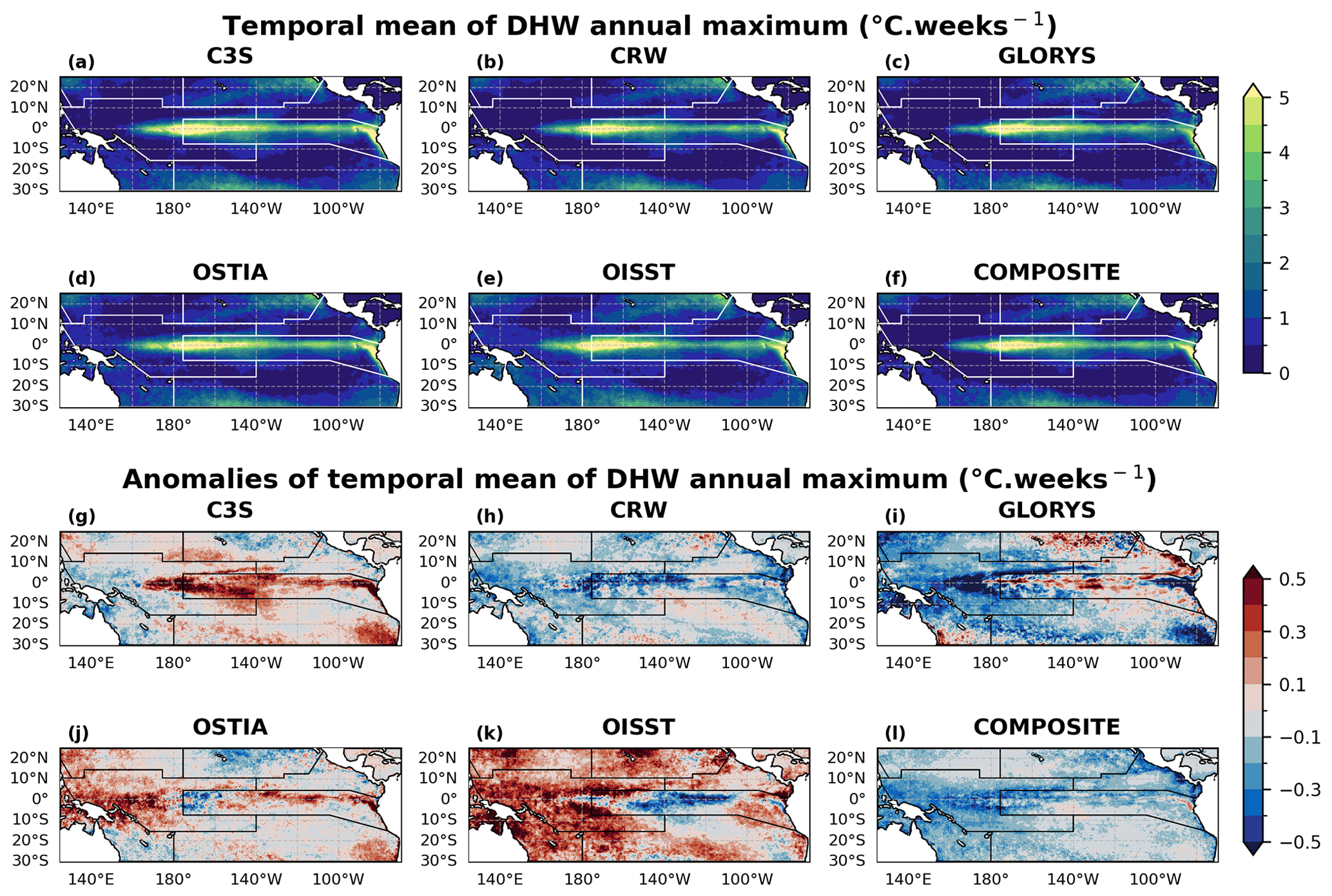
Figure 10 (a–f) Temporal mean of DHW annual maximum over the period 1993–2021 for the six SST products. White lines indicate regions' limits. (g–l) Anomalies of the temporal mean of DHW annual maximum for each product relative to the ensemble mean (Sect. 2.3.1). Black lines indicate regions' limits.

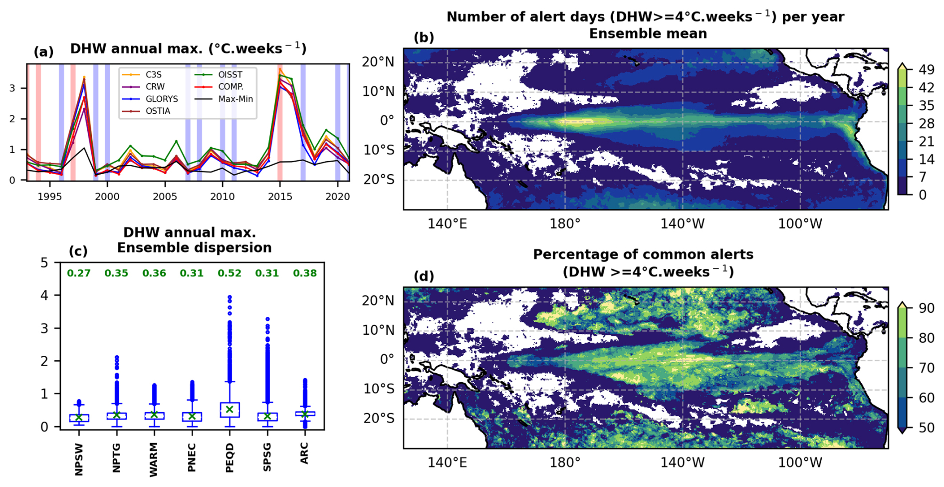
Figure 11 DHW analysis. (a) Yearly time-series of DHW annual maxima averaged over the tropical Pacific for each product. The black line represents the largest inter-product difference value for each year (maximum−minimum). The red and blue backgrounds indicate years of strong El Niño and La Niña, respectively, according to the ONI. (b) Ensemble mean of the number of level 1 alert days (DHW≥4 °C weeks) per year, for each pixel of the tropical Pacific over 1993–2021. (c) Spatial boxplot of ensemble dispersion on DHW annual maxima within the study regions. The green marker represents the mean value, for which the exact value is indicated on top of the associated boxplot. (d) Percentage of common alerts of level 1 between C3S, CRW, OSTIA, OISST and GLORYS12v1.

Figure 11a confirms that over the years, OISST detects the highest annual maxima of DHW, except in years of strong El Niño (1997–1998, 2015–2016) where C3S shows the highest annual DHW maximum (averaged values over the basin). As in Fig. 5, spatial boxplots of ensemble dispersion in DHW annual maxima within each region are represented in Fig. 11c. Across regions, the spatial averages of dispersion (green markers and values in Fig. 11c) range between 0.27 and 0.52 °C weeks, reached in the NPSW and PEQD, respectively. Such uncertainties, with outliers reaching more than 1 °C weeks in all regions except NPSW, appear critical when comparing DHW values to the bleaching level of alert of 4 °C weeks defined by the NOAA (level 1 alert). This is further illustrated in Fig. 11b and d which show the number of level 1 alerts (ensemble mean) in the tropical Pacific, and the associated percentage of common alerts between C3S, CRW, OSTIA, OISST and GLORYS12v1. The spatial average over the basin of the number of level 1 alerts for each product (not shown) revealed that OISST detected the most alerts closely followed by C3S, while the COMPOSITE detected the fewest, closely followed by CRW and GLORYS12v1. These results are in line with the maps of anomalies of Fig. 10g–l and the previous observations. In most of the basin, the proportion of level 1 common alerts i.e. the common days for which DHW≥4 °C weeks across products ranges between less than 50 % and 80 % (Fig. 11d). In large areas of the basin (in ARC, in PEQD close to the south American coast and in PNEC), percentages of common alerts reach 70 % at maximum. They even drop lower than 50 % south of New Caledonia and in the Coral Sea (ARC). This means that among all bleaching alert days in these areas (which range between 1 and 2 weeks per year over 1993–2021 for ARC, Fig. 11b), at least one third or even a half was not detected by at least one of the five products evaluated here. These results confirm that SST product choice is also crucial to the DHW index.

4 Discussion and conclusions

In this study, we have quantified the sensitivity of MHW metrics and DHW index to the SST product chosen in the tropical Pacific over 1993–2021, at both basin and regional scales. Uncertainties associated with the choice of the SST product were assessed using ensemble dispersion for each metric and region.

4.1 Inter-product differences and uncertainties

MHW mean metrics and temporal means of DHW annual maxima show similar spatial patterns in the tropical Pacific across the six SST products evaluated. The observed spatial patterns of MHW metrics are consistent with previous regional (Holbrook et al., 2022; Lal et al., 2025; Pagli et al., 2025) and global MHW studies (Oliver et al., 2021). However, products show significant differences in the absolute values of the mean metrics and DHW index, which can be up to a factor of two between OISST and GLORYS12v1. Over the basin, OISST detects the largest maximum intensity, onset rate, number of events and number of bleaching alerts, but the lowest duration, cumulative intensity and number of MHW days per year. On the opposite, the reanalysis GLORYS12v1 shows the largest number of MHW days per year, duration and cumulative intensity along with the lowest onset rate and second lowest maximum intensity, number of events and number of bleaching alerts. Such behaviors for MHW metrics were also observed by Lal et al. (2025) in the South Pacific island countries and by Wang et al. (2024) in the Northwest Pacific. The observed differences between these two products can be notably related to their strong (OISST) and weak (GLORYS12v1) high-frequency (periods shorter than 2 weeks) SST variability (cf. following section).

Inter-product differences can lead to very different interpretations of the same extreme temperature event. As an example, SST time-series from the six products at one location off the eastern Australian Coast (147° E, 13° S) are shown for 2016 (Fig. 12), when a massive MHW occurred across the Southwest Pacific (Dutheil et al., 2024) causing important damage at the Great Barrier Reef (Great Barrier Reef Marine Park Authority report, 2017). The different time series reveal that this MHW was detected by all products (temperatures are above the 90th percentile from approximately February 2016 to September 2016), but in very different ways (Fig. 12). The number of MHW events detected over the time period ranges from 3 (GLORYS12v1) to 9 (OSTIA), and the cumulative intensity of the MHWs detected from 78.9 °C d (OSTIA) to 182.1 °C d (GLORYS12v1). Consequently, interpretations linked to the biological impacts of such events, (e.g., which metrics have the greatest impact on ecosystems: the number of events? duration? recovery time?) can drastically vary from one SST product to another. Same issue applies to the DHW: for the example of Fig. 12, the level 1 alert for coral bleaching was not reached for C3S (3.34 °C weeks), and maximum DHW barely reached the alert threshold for GLORYS12v1 (4.09 °C weeks) while it largely exceeded it for CRW (5.57 °C weeks). More broadly, the percentage of level 1 bleaching alerts in common between C3S, CRW, OSTIA, OISST and GLORYS12v1 reaches at maximum ∼60 %–70 % in large areas of the tropical Pacific, especially in the ARC and PEQD close to coastal areas, where MHW biological impacts are crucial (Smith et al., 2024). Neo et al. (2023) also showed inconsistency in coral bleaching risk indicators calculated among four temperature datasets (including CRW) in Northwestern and Southeastern Australia. It is worth noting that DHW values computed here are lower than the ones from the NOAA CRW daily 5 km satellite coral bleaching DHW product, probably due to differences in the MMM climatological baseline (the full period 1993–2021 was used in our study while years 1985–1990 plus 1993 only are used for CRW DHW product, Heron et al., 2014).

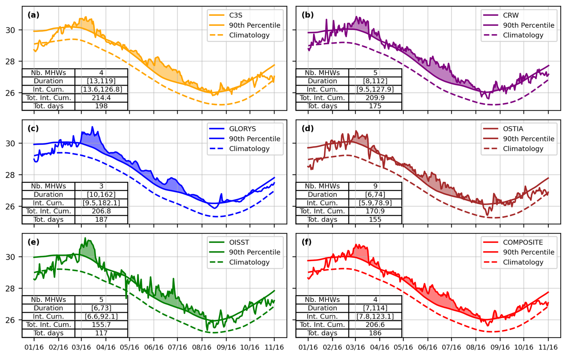
Figure 12 SST time-series of the six products at the same pixel (147° E, 13° S; off the eastern Australian coast) during the MHW event of 2016. The main MHW characteristics identified over the event period (January 2016–November 2016) are indicated in the tables at the bottom left of each panel. Values in brackets represent the minimum and maximum duration and cumulative intensity of the detected events.

Regarding metrics sensitivity to the SST product choice, the onset rate is the most affected metric with the highest ensemble dispersion (between 22.6 % in the ARC and 32.2 % in the WARM) and lowest spatial correlation across all regions of the tropical Pacific. This metric should therefore be considered very carefully in MHW studies, especially since the onset rate determines the reaction window to a MHW, a key index for marine decision makers (Spillman et al., 2021). In contrast, the maximum intensity shows low ensemble dispersion (between 5.2 % in the NPTG and 10.4 % in the WARM) and high ensemble spatial correlation values in all regions, with a low interannual variability of both parameters in all regions, making it a robust metric regarding inter-product SST variability. Metrics with intermediate sensitivity – duration, cumulative intensity, number of events per year and number of MHW days per year – should be considered carefully as their ensemble dispersion, spatial correlation and interannual variability show high spatial differences. Consequently, SST product choice, region and study year might all influence these metrics.

Our results regarding MHW metrics differ from those of Marin et al. (2021). In their coastal MHW analysis, mean intensity – strongly correlated with maximum intensity – showed the largest inter-product differences among the four datasets considered. This discrepancy may arise from several factors. First, methodological differences: Marin et al. (2021) assessed each product's deviation from the ensemble mean metric using a threshold based on ensemble dispersion to identify outliers and hotspot regions of inter-product differences (pixels with at least one outlier product). Such results depend on the individual product and ensemble mean MHW metrics, whereas our study gives an absolute value of the metric uncertainty by solely focusing on the ensemble dispersion. Second, we studied different types of events in different areas: Marin et al. (2021) focused on coastal MHWs worldwide on detrended SST time series while we studied all MHWs in the tropical Pacific without detrending.

Despite differences in metric robustness, our sensitivity analysis revealed that ensemble dispersion decreased and spatial correlation increased over time for all metrics and regions, reflecting the growing coherence between satellite SST datasets (Yang et al., 2021) and hence improvements in reanalysis products such as GLORYS12v1 (which assimilates satellite SST data) over the last decades. The intercomparison study of eight global gap-free SST products by Yang et al. (2021) indeed highlighted that global mean SST time series showed larger differences among products during the early period of the satellite era (1982–2002) when there were fewer observations.

To estimate an uncertainty in MHW metrics and DHW index, our sensitivity analysis also confirms the need for a regional approach, since ensemble dispersion values and their interannual variability vary across regions and metrics. A summary of uncertainties in each region for the six studied MHW metrics is provided in Fig. 5 and in Fig. 11 for the annual maximum of DHW. Within this regional framework, the WARM region particularly stands out across all MHW metrics, with dispersion values among products higher than 10 % of the regional ensemble mean. The SST product considered for MHW analysis should therefore be chosen with caution in this area. Regarding DHW, the PEQD particularly stands out with uncertainty reaching 0.5 °C weeks, which appears crucial when comparing to the level 1 of alert for coral bleaching.

4.2 Potential explanations of these differences

The use of different data sources (satellites with infrared or microwave sensors, geo-stationary or not, use of in situ data or not, and if yes of various types – ships, drifting buoys, moored buoys, Argo), depths of SST estimations (skin layer, foundation), time of SST estimations (dusk to dawn, night-time only, daily mean) and the different data interpolation methods or assimilation methods in the SST products certainly explain the observed inter-product differences (Martin et al., 2012; Dash et al., 2012; Okuro et al., 2014; Fiedler et al., 2019; Huang et al., 2023). The MHW detection and DHW computation methods, both relying on thresholds, then amplifies small differences when computing MHW metrics and DHW.

Our results suggest that MHW detection is particularly sensitive to the high frequency variability of the SST signal. The combined analysis of the standard deviation of the high frequency SST signal (filtered at 15 d) in Appendix A (Fig. A1) and the radar chart of Fig. 3 suggest that spiky signals with stronger high frequency variability like OISST and OSTIA detect higher maximum intensity, onset rate and number of events, but lower duration, cumulative intensity and number of MHW days per year. On the opposite, smoother products like GLORYS12v1 or the COMPOSITE with lower high frequency variability (Fig. A1) detect lower maximum intensity, onset rate and number of events, but higher duration, cumulative intensity and number of MHW days per year (Fig. 3). Thus, the similarity of behaviours between GLORYS12v1 and the COMPOSITE (Fig. 3) might reflect the smoothing effect induced by the multi-product mean SST. These effects of high frequency variabilities were also seen in the SST time series of Fig. 12: climatological levels were similar between products, but OISST and OSTIA signals showed larger high frequency variability (confirmed by Fig. A1), which resulted in the detection of more MHWs of shorter durations (that duration reached 73 and 74 d maximum, respectively, Fig. 12), while GLORYS12v1 or the COMPOSITE showed smoother signals and detected fewer MHWs but of longer durations (duration of maximum 162 d for GLORYS12v1, Fig. 12).

It is also worth noting that the sensitivity of MHW metrics to SST high-frequency variability may partly arise from the event definition itself: changing the minimum duration threshold (≥5 d) or the maximum gap to consider a continuous event (2 d) might affect the inter-product differences. More continuous indices, such as severity (Hobday et al., 2018; Sen Gupta et al., 2020) might help to reduce inter-product differences in MHW diagnostics.

A preliminary work on the impact of re-gridding on the observed inter-product differences was also conducted inside two small areas of the tropical Pacific, and results for the area of New Caledonia are presented in the Supplement (Table S1 and Figs. S8 and S9). The analysis suggests that the re-gridding has little impact on the results of our study but might have an influence on inter-products dispersion for the onset rate metric. C3S and GLORYS also seem to be more impacted by the re-gridding than CRW and OSTIA.

The spatial variability of common MHW days appears to be linked to the spatial scales of MHWs: low (high) percentages of common days correspond to areas with a high proportion of micro (macro) scale events. Indeed, the detection of macro scale MHWs ($>\mathrm{5}\mathit{°}\times \mathrm{5}\mathit{°}$) was shown to be more robust across products compared to micro scale MHWs ($\le \mathrm{5}\mathit{°}\times \mathrm{5}\mathit{°}$), with percentages of common MHW days for macro events largely higher than for micro events. The high proportions of micro MHWs (Fig. 6b) are also located in the areas of larger high frequency variability (Fig. A1): in the coastal areas of the PNEC, NPTG, ARC, in northern NPSW and along the Equator in the PEQD. Also, the duration, cumulative intensity, maximum intensity and onset rate show slightly higher dispersion values for micro-scale events than for macro-scale ones, but large differences are observed for the total MHW days and number of events per year, for which dispersion is higher by a factor of 2 for micro-scale events. Lal et al. (2025) similarly reported strong discrepancies in the number of micro-scale events across products whereas macro-scale events counts were relatively consistent. Consequently, a better understanding of the sensitivity of MHW detection for these spatially small events, as well as an improvement of SST products at these fine scales, might help to reduce the observed inter-product differences.

The spatial correspondence between common MHW days across products and climatological precipitation patterns (i.e high precipitation; low percentages of common MHW days and vice versa) suggests that atmospheric conditions in convective areas of the SPCZ and the ITCZ (Brown et al., 2020) influence MHW detection. This effect may be linked to differences in signal retrieval and the handling of outliers in the presence of clouds and convective rainfall (for instance, there are spurious peaks in OISST induced by clouds, Reynolds et al., 2007). Alternatively, the particularly higher dispersion and lower ensemble spatial correlation values in the WARM region could also be explained by the specific MHW characteristics (short, numerous and spatially confined events that are difficult to detect). Nonetheless, the WARM region also shows the strongest decreasing rate in ensemble dispersion over time, suggesting that the growing coherence among satellite SST products in recent years (Yang et al., 2021) might have improved the detection of these short, small spatial scale and weak amplitude events.

Regarding the relevance of a multi-product approach, our results highlighted that the COMPOSITE does not show an intermediate “ranking” but rather follows the behaviour of the reanalysis product. Metric estimates from the COMPOSITE were influenced by the smoothing applied when averaging temperature data, which introduced biases in MHW statistics.

4.3 Recommendations

Firstly, our results highlight the importance for MHW scientists to understand the behaviour of the SST product selected in their study, particularly its relative “ranking” compared to other products, which varies according to both the metric and the region considered (Sect. 3.2) but also according to the time period of interest (as magnitude of inter-product differences varies between years, Sect. 3.3.3). The evaluation of the high frequency variability of the SST signal can also give valuable information on the product chosen since it influences MHW detection, as explained in Sect. 4.2. Using several products for robustness is thus essential: because all SST products differ in their construction, we cannot a priori argue for a “best” dataset to be used for MHW detection without thorough evaluation against in situ and independent SST dataset. Yet, Fiedler et al. (2019) performed a comparison of SST datasets to in situ data and summed up the key strengths and weaknesses of various analyses compared to the others. Beyond characterizing product behaviour, MHW studies should also account for the uncertainty associated with SST product choice when reporting MHW metric estimates. When feasible, the use of several SST datasets can substantially increase the robustness of the results, by defining upper and lower bounds of metric estimates. The same recommendations apply for DHW studies, with other studies underlining the need to compare indicators of thermal stress from different data sets (Neo et al., 2023; Margaritis et al., 2025).

Our results should also be interpreted carefully at finer scales, such as in coastal areas. Larger differences between satellite SST and in-situ temperature data were observed in coastal regions (Castro et al., 2012; Woo and Park, 2020) compared to the overall accuracy of the SST in the global ocean and offshore regions. Woo and Park (2020) identified relationships between errors and coastal zones of vigorous tidal mixing, shallow bathymetry, and absence of microwave measurements. Significant differences between satellite and in-situ data were also observed in atolls and lagoons (Van Wynsberge et al., 2017).

4.4 Perspectives

Our study focuses on the sensitivity of MHW metrics to the choice of the SST product. Yet, other methodological options not investigated in this study can also strongly impact the MHW estimates. Since trends in SST products show differences (Menemenlis et al., 2025), detrending SST time series might influence our results and should be investigated further. Also, as Smith et al. (2025) highlighted the significant influence of the baseline on MHW results, this choice might impact our conclusions. Choosing other thresholds for MHW detection to focus on the most extreme events (e.g 98th percentile) might also affect the observed inter-product differences. In the same way, other methodologies for characterising MHWs spatial extent (Sun et al., 2023; Pastor et al., 2024) might influence our results. Similar remarks apply to the DHW, for which changing the accumulation window size or anomaly cutoff might impact our results. In addition, the re-gridding of SST datasets onto a common 0.25° grid might also have influenced our results (computing spatial means for re-gridding tends to smooth SST time series), as mentioned in Sect. 4.2 and illustrated in Table S1 and Figs. S8 and S9. Further investigation over the whole area would be needed to thoroughly answer the question of the impact of re-gridding and how much information is lost in the process. Since re-gridding is a common practice in MHW studies, more investigation on the impact of the chosen target resolution could also help to advance MHW research.

As in Fiedler et al. (2019) with SST datasets, the comparison of our results to MHW metrics and DHW computed from in situ and independent data could add valuable information to the study. Such comparison could help understand how the differences between SST products and in situ SST data are translated through the MHW detection algorithm. However, long time series of in situ data allowing computation of the climatological background and thus MHWs are very sparse, and the depths of the estimated SST might differ, adding other biases in MHW metrics comparison. Extending our analysis at global scale could also give additional valuable information to users. For DHW computation, the comparison of our results to existing bleaching observations in some focus areas (as done by Neo et al., 2023, in northwestern and southwestern Australian reefs and Margaritis et al., 2025, in the Caribbean) could help to better understand the differences and similarities in bleaching risk indicators across datasets.

Including other re-analysis products in addition to GLORYS12v1 in our comparison could also be of interest to better understand the impact of the model and data-assimilation system considered in the different re-analyses on MHW detection, including on their vertical extent. This could be done in the framework of the MER-EP (Marine Environment Reanalysis Evaluation Project), a UN-Decade action led by Mercator-Ocean-International. The comparison of MHW metrics between multiple re-analyses could also benefit from the Observing System Experiments done in the framework of the Synergistic Observing Network for Ocean Prediction (SynObs) project (Fujii et al., 2024), if daily outputs are provided. Such comparisons could also help to quantify the influence of ocean observation systems on MHW metrics estimates.

In conclusion, this study reveals significant dispersion in key MHW metrics and provides new information on how the choice of the SST product impacts MHW detection and bleaching indices. This sensitivity should be kept in mind in future research on MHWs and the ecological impact of extreme temperature events, and the use of multiple SST products in such studies should be advocated to increase the robustness of the findings.

Appendix A

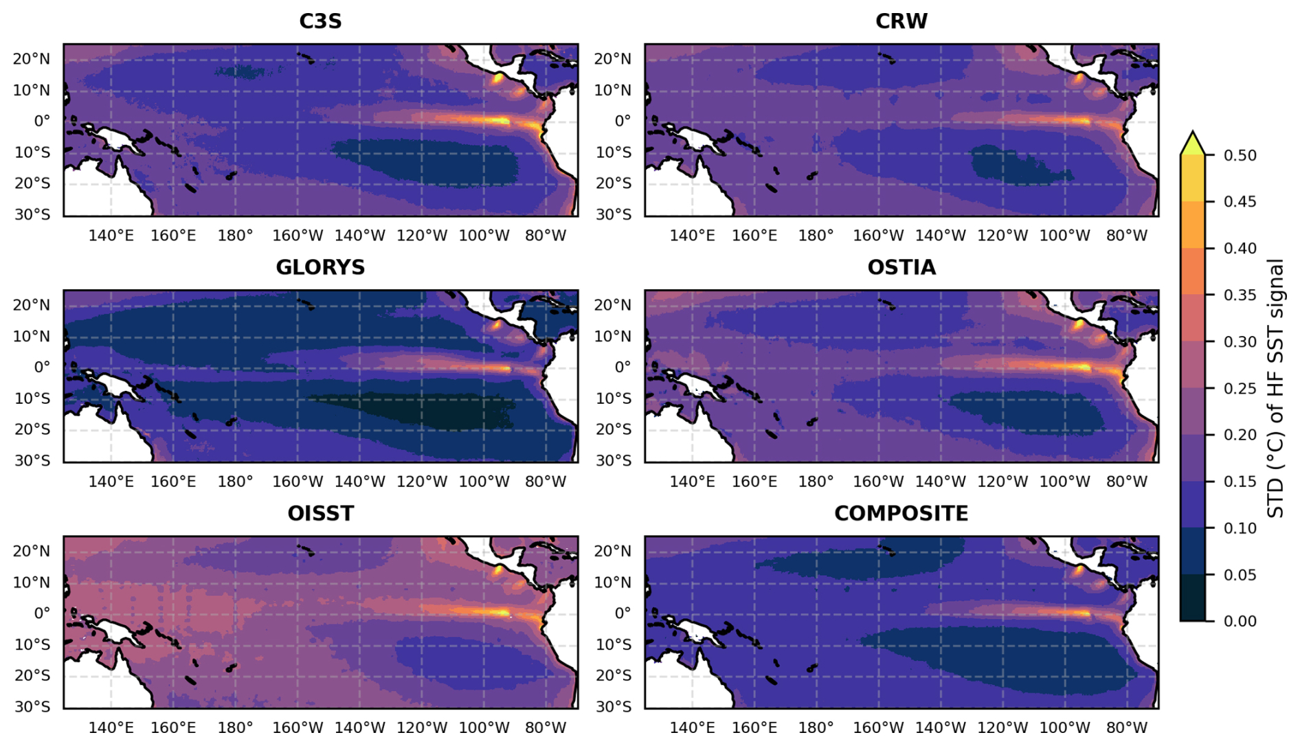
Figure A1 Standard deviation of the high frequency SST signal (high-pass filtered, half-power period of 15 d) over the period 1993–2021 for the six evaluated products.