Polarity and direction dependence of energetic cross-frontal eddy transport in the Southern Ocean's Pacific sector

An example for (a) is a digital elevation model (DEM) purely based on measurement points collected by you and derived by using a software product. If you use an existing map layer from another originator as a basis for significantly enriching the map with your own content, this would be an example for case (b). Mesoscale eddies play a critical role in mediating meridional transport across the Antarctic Circumpolar Current (ACC), yet the dynamics of cross-frontal eddies (CFEs) and their energy exchanges with frontal jets remain inadequately quantified. This study presents a systematic analysis of CFE characteristics, kinetic energy evolution, and thermohaline transport effects in the Pacific sector of the Southern Ocean, utilizing 23 years (2000–2022) of satellite altimetry and Argo float data. Our results reveal a fundamental polarity- and direction-dependent asymmetry in CFE dynamics. Equatorward-propagating cyclonic eddies (CEs) dominate CFE activity, followed by poleward-moving anticyclonic eddies (AEs). These dominant CFE types exhibit superior energetic characteristics, including significantly higher eddy kinetic energy (EKE) and stronger nonlinearity compared to their counterparts. Complete CFEs experience polarity- and direction-selective energy gains during frontal crossing, with equatorward CEs and poleward AEs extracting energy from eastward frontal jets, while their counterparts lose energy. This energization mechanism has intensified over the past two decades, with both polarity CFEs showing substantial EKE increases that substantially exceed previous basin-scale estimates. Hydrographic analysis demonstrates that CEs and AEs transport distinct water masses across frontal boundaries, creating sharp thermohaline contrasts within interfrontal zones. Our findings establish CFEs as crucial regulators that buffer wind- and warming-induced baroclinicity increases through compensatory heat transport, thereby maintaining the Southern Ocean's thermal equilibrium and modulating the ACC's response to external forcing in a changing climate.

1 Introduction

Mesoscale eddies are ubiquitous in the Southern Ocean (SO), play a vital role in the zonal and meridional transport of quantities including heat and momentum across the Antarctic Circumpolar Current (ACC), and also influence the uptake of heat and carbon dioxide from the atmosphere (Moreau et al., 2017; Patel et al., 2019; Sallée et al., 2008; Sokolov and Rintoul, 2007) and the transport and connectivity of marine species (e.g., Duan et al., 2020; Zhu et al., 2025). The ACC comprises multiple zonal fronts, where oceanic jets exit. Here, a front refers to a boundary between distinct water masses, characterized by strong horizontal density gradients, while a jet denotes the narrow, swift current that flows along the axis of such a front. Together, they form the dynamic core of the ACC. At these fronts, mesoscale activity is enhanced, with higher eddy kinetic energy (EKE) and more frequent eddy generation and dissipation (Barthel et al., 2017; Gille, 1994; Hughes, 1995; Hughes and Ash, 2001; Morrow et al., 1994; Sokolov and Rintoul, 2002). In turn, eddies impact the fronts' structure, intensity, and location. For instance, eddies may accelerate the jets, and cyclonic (anticyclonic) eddies cause the equatorward (poleward) deviation of frontal meanders in some cases (Chapman et al., 2020; Duan et al., 2016; Frenger et al., 2015; Sprintall, 2003). These interactions between mesoscale eddies and oceanic fronts can shape local thermohaline structures, exert profound influences on large-scale circulation and vertical flux processes. They also have tremendous implications for the redistribution and survival of marine species and the stability of the climate system.

In the SO, the transition from the warm subtropical waters to the cold Antarctic waters is not smooth but concentrated along a series of fronts (Orsi et al., 1995; Belkin and Gordon, 1996), often corresponding to the locations of narrow, high-speed currents known as “jets” (Sokolov and Rintoul, 2002, 2007). These fronts delineate the boundaries of distinct water masses, each with unique environmental characteristics (Orsi et al., 1995). The existence of fronts hinders meridional exchanges of heat and tracers (Chapman and Sallée, 2017; Naveira Garabato et al., 2011; Thompson and Sallée, 2012). At the same time, eddies enable cross-frontal transport and serve as primary carriers for meridional water mass properties, including heat (De Szoeke and Levine, 1981; Foppert et al., 2017). Cross-frontal eddies (CFEs) must overcome intense geostrophic shear to achieve material transport and render their dynamical contributions to meridional transport, which is significantly more pronounced compared to other eddy types (Thompson and Sallée, 2012).

Eddies' capability of trapping materials and achieving long-distance cross-frontal transport helps in mitigating sharp meridional hydrographic gradients, facilitating new water formation and carbon transport, and also enhancing subsurface temperature extremes in the SO. Holte et al. (2013) presented that cross-frontal exchanges by eddies can penetrate strong potential vorticity gradients associated with the Subantarctic Front (SAF) and facilitate the downstream evolution of Subantarctic Mode Water by transporting cold, low-salinity water across the ACC from the Polar Front Zone (Holte et al., 2013). In a study of a cold eddy in the southwest Indian Ocean, Swart et al. (2008) found that the eddy displaced temperature and salinity anomalies by 1.5° towards lower latitudes. This single eddy contributed 2.5 % of the annual northward flux of Antarctic Surface Water in the southwest Indian sector (Swart et al., 2008). In addition, eddies induce carbon transport across the ACC, which alters the carbon properties and budget of the Subantarctic Zone waters (Moreau et al., 2017). Patel et al. (2019) proposed that about 21 % of the heat transported across the SAF to the Subantarctic Zone south of Tasmania is achieved by cyclonic eddies. He et al. (2023) demonstrated that nearly half of the subsurface temperature extremes in the Southern Ocean occur within eddies, with cross-frontal eddies (CFEs) generating extremely high-temperature events on the cold side of the ACC and extremely low-temperature events on the warm side. These extremes eventually impact marine organisms and ecosystems. For instance, Electrona carlsbergi in the high-latitude Antarctic region may be transported across the fronts from the Argentine Basin by the poleward eddy activity (Saunders et al., 2017; Zhu et al., 2025).

Eddies in the SO can moderate the ACC's response to surface wind forcing changes, namely the “eddy saturation” hypothesis (Hallberg and Gnanadesikan, 2001, 2006; Straub, 1993). Reanalysis of data since 1972 show an increasing trend in wind stress (associated with a positive trend of Southern Annular Mode) over the Pacific sector that dominates the basin-wide wind stress variability, driving enhanced eddy activity responses in this sector, with EKE intensifying at a rate of 14.9 ± 4.1 cm² s⁻² per decade (Duan et al., 2016; Hogg et al., 2015; Menna et al., 2020; Morrow et al., 2010). Recent work by Zhang et al. (2021) demonstrates that EKE intensification is not spatially homogeneous in the SO but concentrated south of New Zealand and downstream of the Campbell Plateau in the Pacific sector. This localized enhancement likely stems from the release of available potential energy stored in tilted isopycnals, thus acting to moderate the eastward flow in the ACC, which has significantly intensified between 48° S and 58° S mainly due to buoyancy forcing (Shi et al., 2021). Mesoscale energy gain from mean flows is achieved through baroclinic (primary) and barotropic (secondary) pathways (Fu et al., 2023). Regarding topographic effects, previous studies have established that interactions between ACC and seafloor topography intensify oceanic eddy mixing by enhancing downstream baroclinic shear. This process enhances eddy generation and increases EKE downstream of major topographic features (Frenger et al., 2015; Morrow et al., 1992; Park et al., 1993; Thompson and Sallée, 2012). Consequently, ACC frontal jets with strong geostrophic characteristics experience mesoscale eddy modulation near prominent topographies (Kim and Orsi, 2014; Thompson et al., 2010).

Despite extensive research on basin-scale EKE modulations and case studies of CFE transport, and the well-established asymmetric eddy distribution on both sides of the ocean fronts, fundamental questions remain regarding how eddy-jet interactions vary based on eddy characteristics and directional approach in the SO. Specifically, it is essential to understand: (1) the polarity and direction preferences of CFEs during frontal crossing; (2) the magnitude and pattern of kinetic energy change within eddies following frontal crossing; (3) the resultant hydrographic property redistribution achieved by CFEs in the interfrontal zones. Motivated by these research gaps, we conducted a systematic assessment of cross-frontal mesoscale eddies in the Pacific sector to elucidate their role in regional ocean dynamics and hydrographic redistribution. Utilizing 23 years (2000–2022) of satellite altimetry data, we characterize the spatiotemporal variability, EKE patterns, and eddy-jet interactions of CFEs in the Pacific sector. We complement these analyses with Argo (Array for Real-time Geostrophic Oceanography) float profiles to quantify normalized hydrographic differences between cyclonic and anticyclonic eddies within the interfrontal zones. These approaches aim to improve our understanding of the dynamic characteristics of CFEs and their role in mediating meridional transport across the ACC in this sector.

2 Data and methods

2.1 Data

This study focuses on the SO's Pacific sector in the range of 150° E–110° W, 35° S–80° S. Prominent topographic features within this region include the Campbell Plateau, Pacific-Antarctic Ridge, Eltanin Fracture Zone, and Udintsev Fracture Zone (Fig. 1). We utilized the gridded satellite altimeter data for eddy detection and tracking. This dataset is merged from multiple satellites and provided by the Copernicus Marine Service as the CMEMS all-satellite L4 SLA product, SEALEVEL_GLO_PHY_L4_MY_008_047 (Copernicus Marine Service, 2024). The data were accessed/downloaded on 18 December 2025 from the Copernicus Marine Service Information (DOI: https://doi.org/10.48670/moi-00148). It includes daily Sea Level Anomaly (SLA) and sea surface geostrophic velocity anomalies (u^′, v^′) data during 2000–2022 with a spatial resolution of 0.125°×0.125°. The SLA represents the sea surface height anomaly relative to the mean sea surface from 1993 to 2012. The corresponding geostrophic velocity anomalies (u^′, v^′) are derived from SLA based on the geostrophic balance (Pujol and Grassi, 2025).

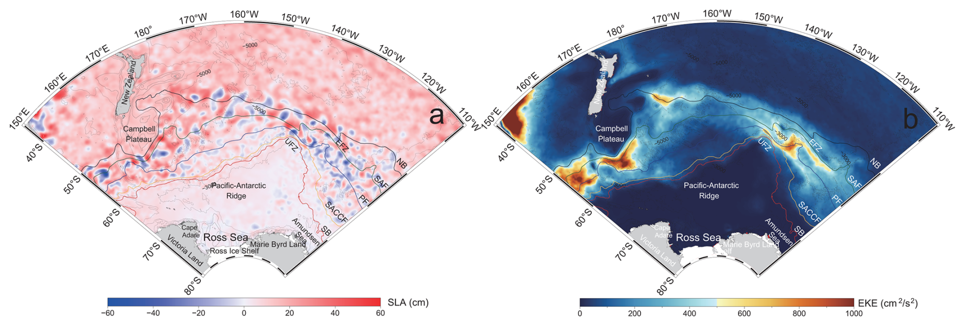
Figure 1 Study region. (a) Sea Level Anomaly (SLA) distribution on 20 January 2022. (b) Spatial distribution of mean eddy kinetic energy (EKE) during 2000–2022. Thick colored lines from north to south represent the northern boundary of ACC (NB), the Subantarctic Front (SAF), the Polar Front (PF), the Southern Antarctic Circumpolar Current Front (SACCF) and the southern boundary of ACC (SB; Park et al., 2019). Significant seafloor topographies have been labeled, with UFZ and EFZ denoting the Udintsev Fracture Zone and the Eltanin Fracture Zone, respectively.

The geographical positions of the ACC's fronts and boundaries used in this study are from the synthesis of Park et al. (2019). This dataset provides the most updated mapping of the ACC frontal system and its associated boundaries, derived from satellite altimetry and independently validated against extensive subsurface observations, including Argo float profiles (2001–2017) and dedicated CTD surveys (2016–2017). As shown in Fig. 1, the dataset defines five major streamlines from north to south: the Northern Boundary (NB), the Subantarctic Front (SAF), the Polar Front (PF), the Southern ACC Front (SACCF), and the Southern Boundary (SB). Specifically, the NB represents the northern dynamical limit of the ACC and coincides with the northern expression of the Subantarctic Front system (SAF-N) in this region. The SAF, PF, and SACCF correspond to the core frontal jets.

Furthermore, a total of 1094 quality-controlled Argo profiles (0–2000 m; https://argo.ucsd.edu/data/, last access: 23 April 2024) located within detected eddies were utilized to analyze the internal thermohaline structure of cyclonic (CEs) and anticyclonic eddies (AEs) The potential temperature (θ) and salinity (S) within each eddy were normalized radially by binning profiles according to their relative distance from the eddy center (normalized by the eddy radius, R), at an average interval of 0.03R. Owing to limited spatial coverage, profiles from the SB-SACCF zone and areas south of the SB were excluded. Consequently, the analysis focused on the northern inter-frontal zones of SAF-NB, PF-SAF, and SACCF-PF, which contained 400, 150, and 252 profiles, respectively. Furthermore, temporal variability (e.g., interannual and seasonal) was not considered in this composite analysis due to the uneven distribution of profiles over time.

2.2 Eddy detection, tracking and CFE categorization

We combined the Okubo-Weiss (OW) parameter method with the outermost closed contour of SLA to detect eddies. As a widely used eddy detection method, the OW parameter method was developed based on flow field deformation by high vorticity or high strain (Okubo, 1970; Weiss, 1991). The OW parameter is defined as:

$$\begin{array}{}\text{(1)}& W=s_{\mathrm{n}}^{\mathrm{2}}+s_{\mathrm{s}}^{\mathrm{2}}-{\mathit{\omega }}^{\mathrm{2}},\end{array}$$

where $s_{\mathrm{n}}=\frac{\partial u^{\prime }}{\partial x}-\frac{\partial v^{\prime }}{\partial y}$ and $s_{\mathrm{s}}=\frac{\partial v^{\prime }}{\partial x}+\frac{\partial u^{\prime }}{\partial y}$ are the normal and shear components of strain, respectively, and $\mathit{\omega }=\frac{\partial v^{\prime }}{\partial x}-\frac{\partial u^{\prime }}{\partial y}$ is the relative vorticity of the flow. The sign of W determines a region to be strain-dominated (W > 0) or vorticity-dominated (W < 0). Eddies are highly vorticity-dominated circulations, thus corresponding to coherent negative-W areas (for both CEs and AEs), and the negative W must be larger than that for the background field (Henson and Thomas, 2008).

To identify physically consistent eddy boundaries, we adopt the hybrid geometric–physical approach validated by Saraceno and Provost (2012), which avoids common biases associated with fixed W thresholds. A threshold of W < −0.2 σ_w is often used to delineate eddy boundaries, with σ_w being the standard deviation of W over the entire region (e.g., Henson and Thomas, 2008; Isern-Fontanet et al., 2006; Frenger et al., 2015). However, this method can underestimate eddy area in certain regions (Matsuoka et al., 2016) and misidentify meanders as eddies in energetic frontal zones (Saraceno and Provost, 2012). Our approach proceeds as follows: after detecting the eddy center using the OW-based method, we identify the outermost closed SLA contour that encloses this point. This contour defines the eddy boundary, and the center was then recalculated as its geometric centroid. Eddy radius was computed as the radius of a circle of equivalent area, and eddy amplitude is the absolute SLA difference between the center and along the contour.

For eddy tracking, the algorithm identifies eddies at time t + 1 that meet the following criteria relative to time t: (1) minimal centroid distance, (2) identical polarity (i.e., rotation direction), and (3) the minimum radius variation. If no eddy at t + 1 satisfies these proximity thresholds for a given eddy at t, the eddy is considered dissipated. Conversely, if an eddy detected at t + 1 does not match any eddy at t, it is classified as a newly generated eddy.

To ensure statistical robustness, our analysis focused exclusively on significant mesoscale eddies, which were defined as well-resolved, energetic eddies with sufficient temporal coherence. Eddies meeting all of the following criteria were retained as the core dataset for subsequent analyses: (1) radius > 30 km; (2) amplitude > 5 cm; and (3) lifespan > 14 d.

The EKE was computed from geostrophic velocity anomalies using the equation EKE$=({u^{\prime }}^{\mathrm{2}}+{v^{\prime }}^{\mathrm{2}})/\mathrm{2}$. In this study, except for Fig. 1, all analyses of EKE variation during cross-frontal processes were based on the total EKE within each eddy interior (EKE_T) for better tracking EKE changes in specific eddies, calculated as ${\mathrm{EKE}}_{\mathrm{T}}={\sum }_{i=\mathrm{1}}^N{\mathrm{EKE}}_i\cdot \mathrm{d}s$, where EKE_i is the EKE for grid i, N is the grid amount within an eddy, and ds is the grid area. The eddy nonlinearity parameter (β) was computed based on $\mathit{\beta }=U/C$, where U is the maximum circum-average geostrophic velocity within the eddy, and C represents the eddy's transporting speed (Chelton et al., 2011). The eddy is nonlinear when β > 1, indicating the presence of trapped fluid parcels advected with the eddy movement.

While climatological fronts define the ACC's mean structure (Park et al., 2019), their positions exhibit meridional variability influenced by both bathymetry and eddy activity (Kim and Orsi, 2014; Thompson et al., 2010). Fronts stabilize over major bathymetric features (e.g., the Pacific-Antarctic Ridge) but show maximum variability in flat basins. Due to eddy-mean flow interaction processes, frontal zones become greater downstream of topographic obstacles like the Campbell Plateau. Based on the observed frontal variability in the Pacific sector, the maximum total meridional frontal drift during 1993–2010 is approximately 80 km southward (at 150° E), and annual cycle amplitude is < 40 km (Kim and Orsi, 2014). To account for these frontal displacements, we first defined a baseline frontal zone as a ±15 km strap in the normal direction from each climatological front. Then, to objectively identify eddy-front interactions, we applied a geometric criterion: an eddy was considered interacting when its boundary contacted the frontal zone. Since all analyzed eddies have a radius (R) > 30 km, this criterion effectively creates a dynamic interaction zone with a minimum half-width of 45 km (15 km + 30 km), which comfortably exceeds the observed ranges of frontal variability. To further ensure robustness, we conducted a sensitivity analysis by expanding the frontal zones to a ±25 km strap (see Supplement), which confirmed that all key findings are insensitive to the exact zone definition.

The eddy-front interaction was then divided into three sequential phases: pre-cross-frontal, cross-frontal, and post-cross-frontal. CFEs were further categorized into four types: (1) Front-generated eddies, generated within the dynamic interaction zone and subsequently propagating away, (2) Front-dissipated eddies, propagating into the dynamic interaction zone and dissipated there, (3) Transient frontal eddies, both generated and dissipated within the same interaction zone, and (4) Complete CFEs, undergoing all three phases (pre-, cross-, and post-frontal) relative to the dynamic interaction zone. Both types (1) and (2) eddies were collectively classified as partial CFEs. Hereafter, all frontal zones refer to dynamic interaction zones. Notably, according to the definition, the partial frontal crossing eddies of Type 1 include rings pinched off from the meandering structures of a front.

3 Results

3.1 Analysis of CFE characteristics

CFE transport is active across all major ACC frontal zones in the Pacific sector (Fig. 2). At each front, equatorward-moving CFEs consistently outnumber poleward-moving eddies (Fig. 2b). CEs dominate equatorward CFEs, with CEs outnumbering AEs by a factor of ≥ 1.5, while AEs prevail in poleward CFE motions. The resulting hierarchy of CFE prevalence is as follows: equatorward CEs are the most frequent (36 % of total CFEs), followed by poleward AEs (30 %) and equatorward AEs (18 %), with poleward CEs (16 %) being the least frequent. Among the different frontal zones, the SAF hosts the most eddy occurrences (30 % of total CFEs), followed by the PF (27 %), reflecting intense eddy-mean flow interactions around these two fronts. The northernmost NB (23 % of total CFEs) and the SACCF (16 %) exhibit comparable and moderate CFE levels, while the southernmost SB (7 %) displays the lowest CFE exchanges.

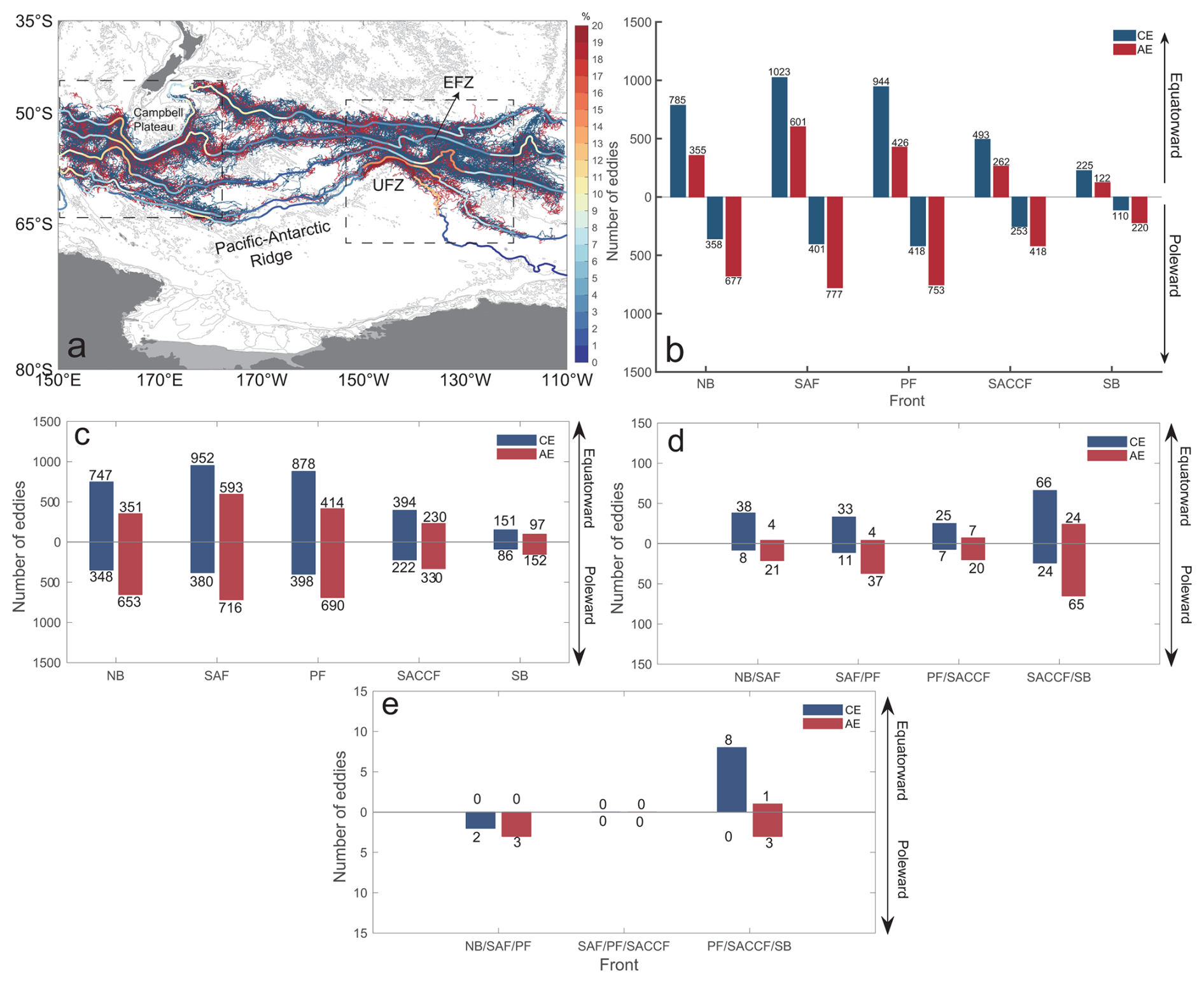
Figure 2 CFE trajectories and statistics of eddy counts. (a) CFE trajectories. The color along each front represents the relative occurrence of CFEs (%) per 5° latitudinal bin. The framed regions denote the area where active CFE activity occurs. (b) Total number of CFEs, divided into types of equatorward and poleward directions, shown as a function of the different ACC fronts; (c–e) Numbers of single-, double-, and triple-frontal crossing CFEs, respectively. Red represents anticyclonic eddies (AEs) and dark blue denotes cyclonic eddies (CEs).

The frontal system exhibits strong meandering patterns due to topographic steering, accompanied by spatially heterogeneous CFE distributions. CFE occurrence peaks downstream of prominent topographic features, particularly near the Campbell Plateau (150° E–180° E; 41 % of total CFEs) and downstream of the Udintsev Fracture Zone (125° W–160° W; 38 %), where multiple fronts converge (Fig. 2a). Eddies may cross multiple fronts sequentially at these frontal convergent regions. The majority of eddies cross a single front (Fig. 2c). Double-frontal crossings (total 411) occur preferentially at southern fronts (SACCF/SB; > 50 % of cases; Fig. 2d). Triple-frontal crossings are rare and primarily limited to the PF/SACCF/SB system (Fig. 2e), and no instances of quadruple-frontal crossings were observed.

Consistent with the ACC dynamics, over 70 % of cross-frontal CEs and AEs propagate eastward (Fig. 3), a notable contrast to the typical westward propagation of mesoscale eddies driven by Rossby waves in other ocean basins (Frenger et al., 2015). Short-distance movements (< 2°) are more frequent for AEs at each front. In contrast, CEs dominate long-distance propagation, particularly at the SAF and PF. The majority of CEs propagate northward (over 64 % of all CEs), while over 54 % of AEs are oriented southward. The greater energetic content of CEs, as indicated by their dominance in long-distance transport, aligns with their role as primary agents of meridional exchange. These patterns highlight how ACC-steered eddy motions facilitate distinct transport pathways, with CEs disproportionately driving long-distance exchanges, particularly at major fronts such as the SAF and PF.

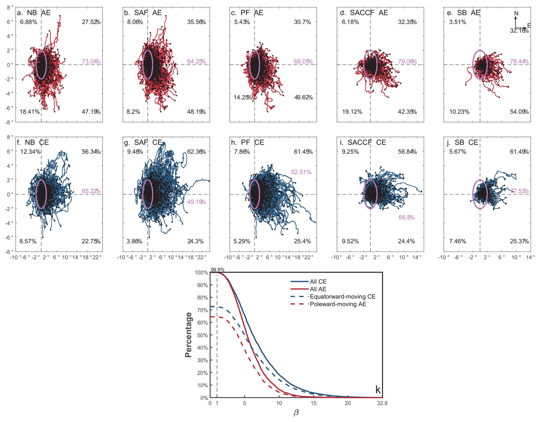
Figure 3 Relative movement trajectories of CFEs (a–j) and the percentage distribution of eddy nonlinearity β (k). In (a–j), black percentages represent the proportion of eddies moving in different quadrant directions calculated based on the end point of the trajectory, and purple percentages indicate the proportions of eddies with movement distances within a 2° range, with the coordinate origin (0°, 0°) denoting the eddies' generation locations. Note that eddies crossing multiple fronts may appear repeatedly at different frontal positions in this analysis.

Most CFEs (99 %) exhibit nonlinear characteristics (Fig. 3k), confirming their capability to trap and advect water mass during their lifespan. In the nonlinearity regime (β > 1), equatorward-moving CEs constitute 72.6 % of the total cross-frontal CEs, and 64.5 % of the total cross-frontal AEs are poleward-moving ones (Fig. 3k). In the high nonlinearity regime (β > 5), the proportion of CEs is notably higher than AEs, consistent with the greater dynamic vigor of CEs observed in the above analyses. Therefore, the cross-frontal transport achieved by eddies, primarily equatorward-moving CEs and poleward-moving AEs, can facilitate the redistribution of distinct source water masses and reduce thermohaline gradients across frontal zones.

Cross-frontal CEs and AEs show similar distributions in lifespan, propagation distance, and size (Fig. 4). Both types show a steep decline in abundance with increasing lifespan. Eddies with lifespans ≤ 50 d dominate, constituting 55 % of the total eddy population, while only 3 % exceed 200 d (Fig. 4a). Propagation distances are confined predominantly to ≤ 400 km (56 % of total CFEs). CEs slightly outnumber AEs at longer distances (400–1000 km; Fig. 4b). Size distributions reveal that ∼ 75 % of the total sample have mean radii of 30–50 km (Fig. 4c). Notably, CEs dominate at smaller radii (< 50 km), while AEs prevail among larger eddies. This distribution pattern is consistent with maximum radius statistics (Fig. 4d). These CFE characteristics align with previously reported eddies in the Pacific sector (Duan et al., 2016).

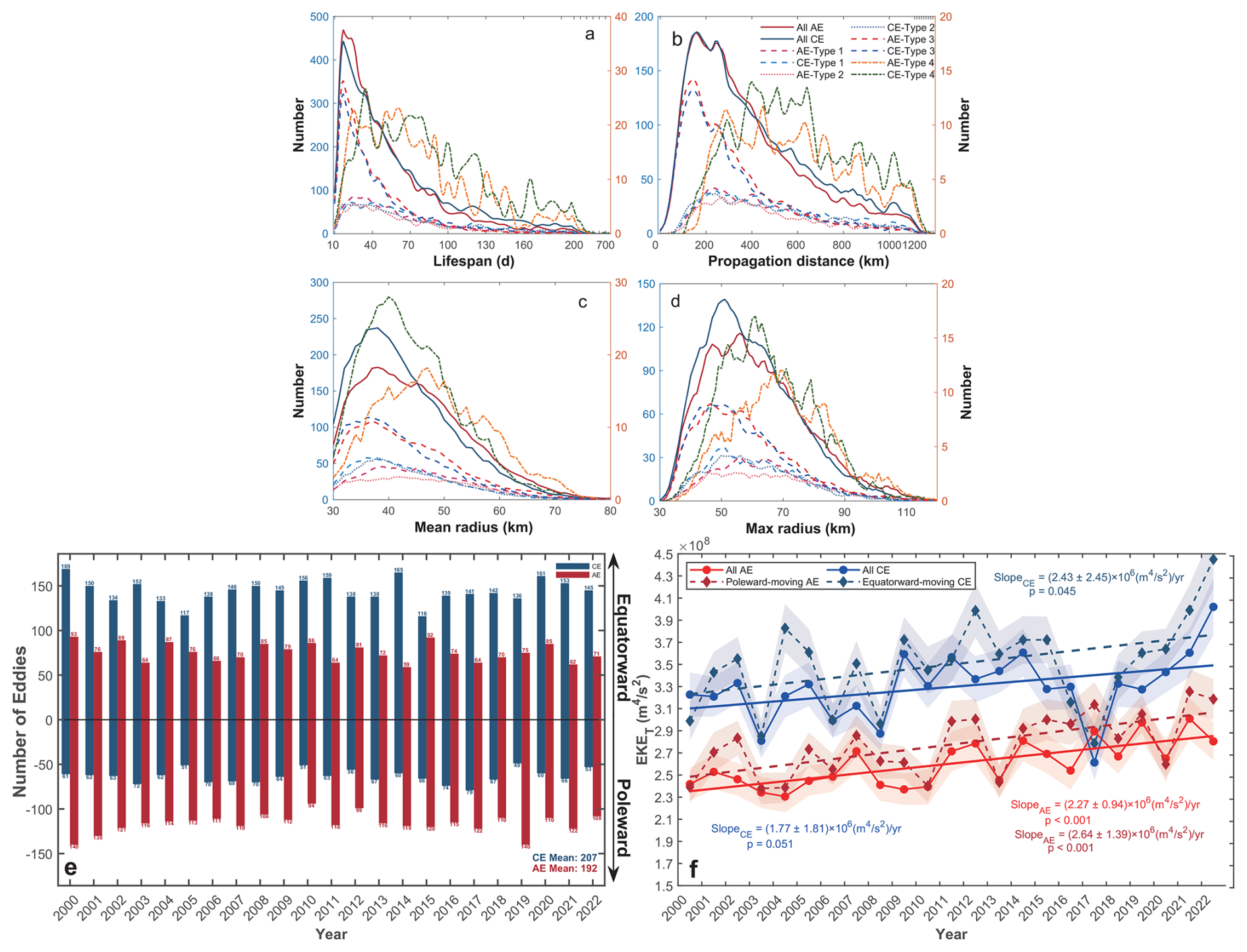
Figure 4 Statistical characteristics of different types of CFEs (a–d), time series of annual CFE counts (e), and annual mean EKE_T (f). Eddy counts according to (a) eddy lifespan, (b) propagation distance, (c) mean radius over lifespan, and (d) maximum radius in the lifespan. In (a–d), “All” represents all CFEs, “Type 1” denotes eddies front-generated and subsequently transported away, “Type 2” indicates eddies transported into the frontal zone and dissipated there, “Type 3” represents eddies generated and dissipated within the same frontal zone, and “Type 4” shows complete CFEs experiencing pre-crossing, crossing and post-crossing phases. The left y-axis is for the first three subsets, and the right axis is for the Type 4 eddies to clarify their distribution. The x-axes in (a) and (b) are compressed at higher values. In (e), all-year mean counts of CEs and AEs are indicated at the bottom right. In (f), the annual mean EKE_T for all AEs and CEs and the linear trends are depicted by dots, red and blue solid lines, respectively. The extracted subsets of poleward-moving AEs and equatorward-moving CEs are depicted by diamonds, red and blue dashed lines, respectively. Error shadings represent ±1 standard deviation, and slope values are given with ±95 % confidence intervals.

Subsequently, we found distinct characteristics among types regarding their behaviors, when dividing the CFEs into partial CFEs, generated within and subsequently transported away (Type 1) and transported into and dissipated within the frontal zones (Type 2); transient CFEs, both generated and dissipated within the same frontal zone (Type 3); and complete CFEs, experiencing pre-crossing, crossing, and post-crossing phases (Type 4). Transient CFEs dominate numerically, accounting for 48 % of all CFEs, and partially generated and dissipated CFEs constitute 23 % and 20 %, respectively (Fig. 4a–d). These proportions collectively indicate that the frontal zones primarily act as terminal/starting areas for eddy life cycles, rather than a simple transit pathway. The proportion of transient CFEs falling within low-value parameter ranges is substantially higher than that of the other types: 59 % of these eddies have lifespans ≤ 40 d and propagation distances ≤ 300 km, as well as 58 % have mean radius ≤ 43 km and 63 % have maximum radius ≤ 60 km. These values confirm the intrinsic nature of transient eddies as “generated and dissipated locally”, and reveal the constraining role of the frontal system on eddy evolution. In stark contrast, completely transported CFEs exhibit markedly different dynamical characteristics: 81 % have lifespans > 40 d, 90 % propagate > 300 km, and 68 % have maximum radii > 60 km, indicating that these eddies have completely escaped the constraints of the local frontal environment and possess the capability for long-distance cross-frontal transport. Notably, among completely transported CFEs, small-scale CEs dominate significantly, with CEs accounting for 63 %, while AEs account for only 37 % for eddies with mean radii of 30–50 km and maximum radii < 70 km. This polarity bias suggests that small-scale CEs may possess higher transport efficiency in cross-frontal material and energy exchange due to their unique dynamical structure.

Quantitative analysis of CFE types reveals distinct frontal-zone behaviors (Table 1). Transient eddies (Type 3) account for the largest proportion overall (> 40 % by summing the transient AEs and CEs at each front), particularly at the two weaker southern fronts (SACCF and SB). Their proportions are lower at the SAF and PF, indicating that these two major fronts host more eddies that interact with areas outside the frontal zone during their lifecycle. For partially front-generated eddies (Type 1), both AEs and CEs exhibit relatively high proportions at the SAF and PF. At the southern SACCF and SB, however, the proportion of AEs drops markedly, whereas CEs show no such reduction. Among partially front-dissipated eddies (Type 2), the three northern fronts consistently show a higher proportion of CEs than AEs. At the two southern fronts, the pattern reverses, CE proportions decline sharply, causing a higher proportion of AEs. This suggests that in the southern fronts, local cross-frontal CEs are more readily generated and propagated outward, while being relatively resistant to dissipation.

Table 1 Proportions of numbers of different eddy types relative to the total number of CFEs at each frontal zone.

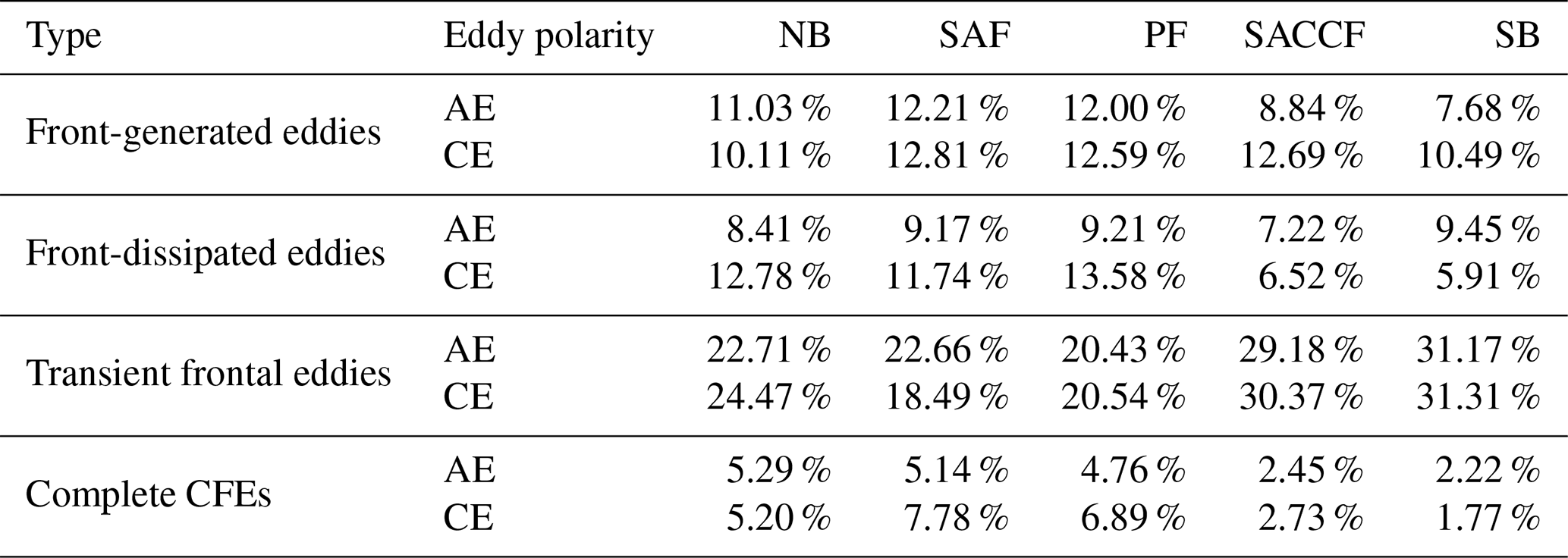
Regarding the partial CFEs, the proportion of front-generated AEs consistently exceeds that of front-dissipated AEs (except the SB), indicating that AEs are more likely to be generated within the fronts than to dissipate locally, particularly at the three northern fronts. For complete CFEs (Type 4), the proportion of AEs decreases with frontal latitude, while CEs reach their maximum proportions at the SAF and PF. These results demonstrate that different CFE types exhibit distinct behaviors when interacting with each front, shaped by frontal dynamics and latitudinal position.

Over the 23 years, the counts of poleward- and equatorward-moving eddies show pronounced interannual variability (Fig. 4e). The annual abundance hierarchy, equatorward CEs > poleward AEs > equatorward AEs > poleward CEs, mirrors the total distribution in Fig. 2b. In terms of EKE_T, CEs consistently exhibit approximately 1.5-fold greater EKE_T than AEs (Fig. 4f), consistent with their longer propagation distances and higher nonlinearity (Fig. 3). While the increasing trend in CEs' EKE_T is not statistically significant overall (1.77 ± 1.81) × 10⁶ m⁴ s⁻² yr⁻¹ (p = 0.051), this result is influenced by an anomalously low value in 2017, coinciding with an EKE minimum reported by Fu et al. (2023) in the central Pacific sector. Excluding this outlier yields a significant trend of (2.27 ± 1.45) × 10⁶ m⁴ s⁻² yr⁻¹ (p = 0.003). In contrast, AEs' EKE_T displays a robust increase by (2.27 ± 0.94) × 10⁶ m⁴ s⁻² yr⁻¹ (p < 0.001). These results indicate that both eddy polarities contribute to the long-term EKE_T rise, with CEs exhibiting greater interannual variability. As established in Fig. 2, equatorward-propagating CEs and poleward-propagating AEs dominate cross-frontal eddy abundance. Their EKE_T signals are substantially stronger than those of the overall CFE population, with significant increasing trends of (2.43 ± 2.45) × 10⁶ m⁴ s⁻² yr⁻¹ (p = 0.045) for equatorward CEs and (2.64 ± 1.39) × 10⁶ m⁴ s⁻² yr⁻¹ (p < 0.001) for poleward AEs. Thus, beyond their numerical dominance, these two subsets also govern the EKE level of CFEs and its intensification over the study period.

More specifically, all CFE types exhibit pronounced interannual variability and follow the same abundance hierarchy observed in Fig. 4e in annual counts, with CEs dominating equatorward-moving eddies and AEs prevailing among poleward-moving ones (Fig. 5a–d). Among the four types, complete CFEs of both polarities show the largest annual mean EKE_T, and display statistically significant increases over the study period with (4.16 ± 3.54) × 10⁶ m⁴ s⁻² yr⁻¹ (p = 0.024) for CEs and (3.17 ± 2.49) × 10⁶ m⁴ s⁻² yr⁻¹ (p = 0.015) for AEs, respectively (Fig. 5h). The dominant contributors to this enhancement are the same subsets that dominate abundance, equatorward-moving CEs and poleward-moving AEs, underscoring their role as the primary EKE_T source for complete CFEs. In contrast, partial and transient CFEs exhibit substantially lower EKE_T levels, with transient eddies showing the weakest energy content. Most of their increasing trends are not statistically significant (Fig. 5a–c), with the notable exception of transient AEs, which display a significant EKE_T increase (Fig. 5c).

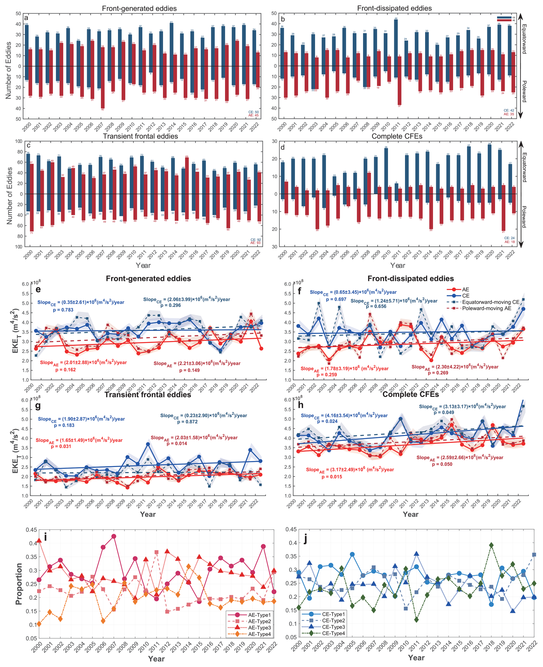
Figure 5 Annual statistical characteristics of four types of CFEs, including their counts, mean EKE_T, and proportions of the summed EKE_T relative to all EKE_T. Time series of annual counts for (a) Front-generated eddies (Type 1), (b) Front-dissipated eddies (Type 2), (c) Transient frontal eddies (Type 3), and (d) Complete CFEs (Type 4). (e–h) Annual mean EKE_T for these four types of eddies. (i, j) Annual summed EKE_T for each type relative to all EKE_T for total CFEs. In (a–d), all-year mean counts of CEs and AEs are indicated at the bottom right. In (e–h), the annual mean EKE_T for all AEs and CEs and the linear trends are depicted by dots, red and blue solid lines, respectively. The extracted subsets of poleward-moving AEs and equatorward-moving CEs are depicted by diamonds, red and blue dashed lines, respectively. Error shadings represent ±1 standard deviation, and slope values are given with ±95 % confidence intervals.

The relative contribution of each type to the total annual EKE_T reveals distinct energy compensation patterns between AEs and CEs (Fig. 5i, j). For AEs, the primary energy compensation occurs between Type 1 (front-generated) and Type 4 (complete frontal-crossing) eddies (correlation coefficient R = −0.59; p = 0.003), indicating that enhanced activity of partially frontal-generated AEs tends to suppress complete frontal-crossing AEs, and vice versa. A secondary compensation is between Type 2 and Type 3 (R = −0.46; p = 0.027). For CEs, the dominant compensation is between Type 3 (transient) and Type 4 (complete) eddies ($R=-\mathrm{0.66}$; p < 0.001), with a modest compensation between Type 1 and Type 4 (R = −0.44; p = 0.032). These results suggest that more energetic complete CFEs tend to coexist with reduced activity of either partially frontal-generated or transient eddies. This compensatory relationship is critical for understanding mesoscale eddy-front interactions, particularly during the period of elevated EKE_T in complete CFEs.

3.2 EKE_T evolution of complete CFEs during frontal crossing

Although only a small fraction of eddies complete full cross-frontal transport (Table 1; Fig. 5), these energetic features, originating in non-frontal zones and crossing entire frontal boundaries, likely dominate long-distance heat and material exchange between inter-frontal zones. Their rising EKE_T underscores their increasingly important dynamic role, motivating a closer examination of EKE_T evolution during frontal crossing. The Southern Hemisphere's intrinsic vorticity asymmetry (clockwise CEs vs. counterclockwise AEs) creates fundamental polarity differences in energy exchange when interacting with eastward frontal jets. Consequently, eddies of opposing polarities and directions are expected to exhibit distinct patterns of EKE_T variability during the cross-frontal transport.

Complete CFEs at the northern ACC fronts, NB, SAF, and PF, exhibit substantially higher EKE_T than those at the southern fronts (SACCF, SB; Figs. 6, 7), consistent with their more frequent occurrence at the northern fronts (Table 1). For instance, mean EKE_T at the SAF (4.21 × 10⁸ m⁴ s⁻²) exceeds that at the SB (9.51 × 10⁷ m⁴ s⁻²) by 3.26 × 10⁸ m⁴ s⁻². During frontal crossing, EKE_T evolution exhibits clear polarity- and direction-dependence. Poleward-moving AEs consistently gain kinetic energy during crossing (3.23 %–88.02 % increase), and experience further post-crossing amplification at the three northern fronts (43.52 %–71.76 %), indicating sustained energy extraction from the mean flow (Fig. 6; Table 2). In contrast, poleward CEs subsequently lose energy both during and after crossing, with reductions of 31.22 %–72.74 % in the post-crossing phase. Equatorward-moving CFEs exhibit opposing behaviors (Fig. 7; Table 2). AEs consistently lose energy, showing reductions of 2.59 %–27.47 % during frontal crossing and further decline post-crossing (by 18.41 %–69.02 %). In contrast, CEs generally gain energy, with post-crossing increases of 48.13 %–76.70 % at the four northern fronts. This pattern reverses at the SB, where CEs show subsequent EKE_T loss (e.g., 43.02 % decrease after crossing).

Table 2 Changes in mean EKE_T during different phases for complete cross-frontal eddies (CFEs) relative to pre-crossing values (+: increase; −: decrease). Crossing phases represent when eddies are in the frontal zones, while post-crossing phases indicate when eddies are moving away from the frontal zones. “–” denotes no data.

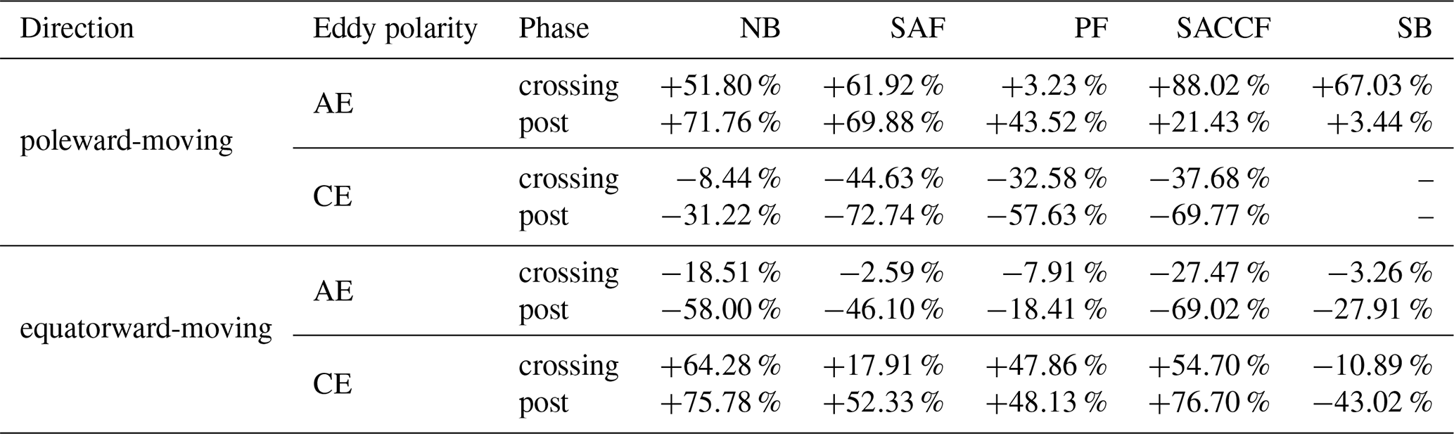
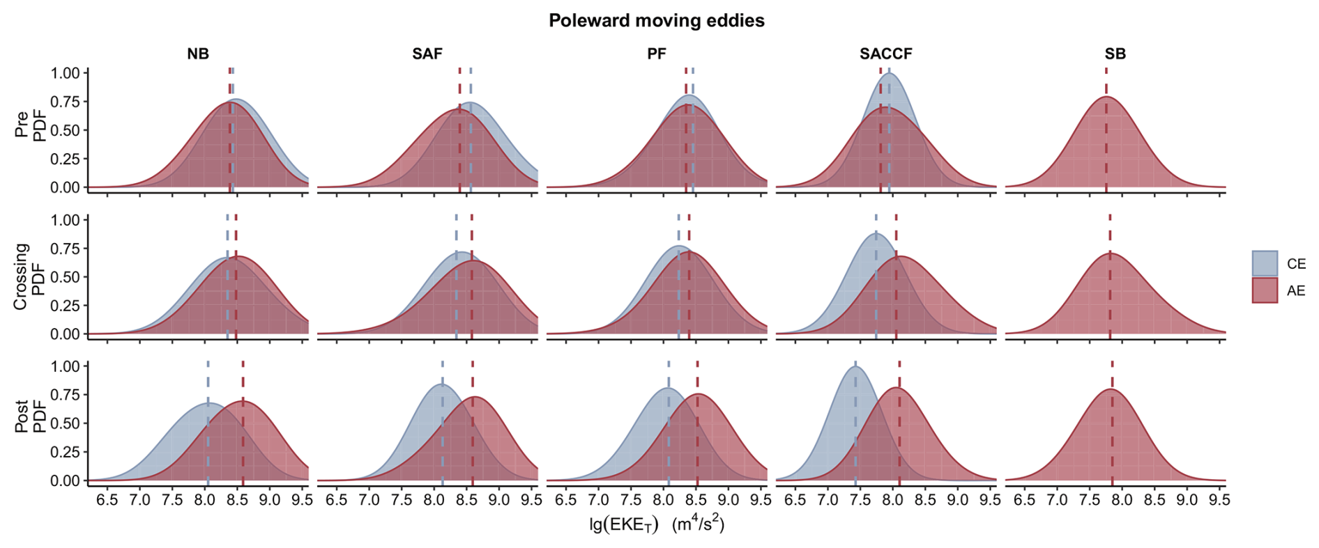
Figure 6 Probability density function (PDF) of EKE_T for poleward-moving CFEs in pre-crossing, crossing, and post-crossing phases. Dashed lines indicate median EKE_T values. Blue and red colors represent CEs and AEs, respectively.

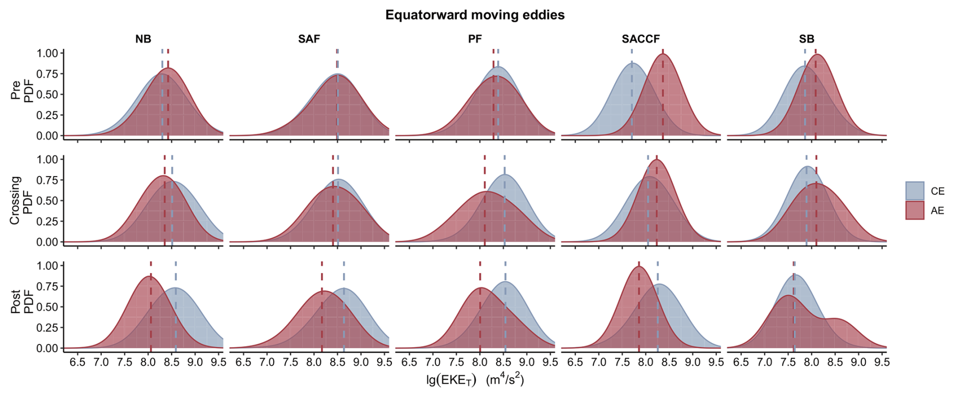
Figure 7 Probability density function (PDF) of EKE_T for equatorward-moving CFEs in pre-crossing, crossing, and post-crossing phases. Dashed lines indicate median EKE_T values. Blue and red colors represent CEs and AEs, respectively.

These results highlight fundamental asymmetries in eddy-front energy exchange governed by eddy polarity, movement direction, and frontal latitude. They also elucidate the energy compensation observed between frontal-generated partial/transient eddies and complete CFEs (as shown in Fig. 5i, j): greater vorticity release to complete CFEs intrinsically reduces local eddy generation. Thus, the energy extraction from frontal jets fuels the complete frontal-crossing equatorward CEs and poleward AEs, contributing to their enhanced post-crossing energetics, consistent with the mesoscale principle of potential vorticity conservation. The anomalous energization of equatorward CEs at the SB, as well as lower post-crossing EKE_T relative to in-crossing values for poleward AEs at SACCF and SB, is likely related to the weaker dynamical but stronger hydrographic characteristics of these southernmost fronts (Park et al., 2019; Thorpe et al., 2002; Vereshchaka et al., 2021).

3.3 Thermohaline transport effects of CFEs

Argo θ–S profiles (Fig. 8) reveal that cyclonic eddies (CEs) and anticyclonic eddies (AEs) exhibit distinct, polarity-dependent hydrographic signatures within the same interfrontal zones. CEs consistently contain colder, fresher water with shallower isopycnals (upper 1000 dbar), whereas AEs are characterized by warmer, saltier water and deeper isopycnals. These contrasts underscore the role of nonlinear eddies in mediating cross-frontal exchange. However, a subset of AEs in the SACCF-PF zone trap anomalously cold, fresh polar waters (θ_min = −1.76° C and S < 34.0 psu), similar to those observed in some AEs within the SB-SACCF zone, indicating that AEs can also transport polar waters equatorward. Notably, eddy-induced vertical motions, upwelling in CEs and downwelling in AEs, produce vertical displacements but do not alter θ–S properties of source water columns (Falkowski et al., 1991; Li et al., 2022a). Therefore, this mechanism can only account for overlapping θ–S signatures that arise from vertical repositioning of the same water mass, rather than true cross-frontal modification.

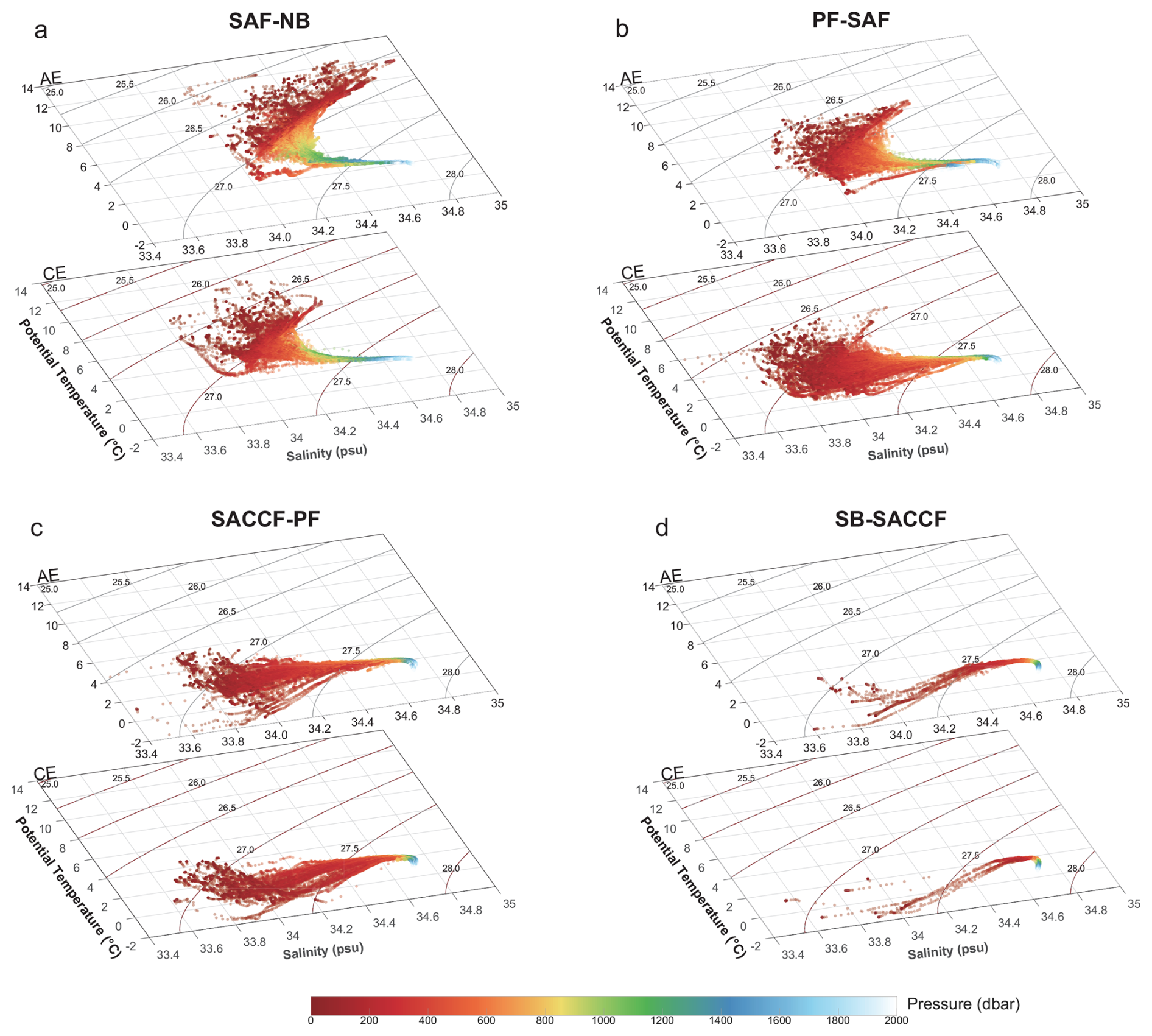
Figure 8 Potential temperature-salinity (θ–S) diagrams in the eddy interiors observed in different inter-frontal zones. (a) SAF-NB; (b) PF-SAF; (c) SACCF-PF; (d) SB-SACCF.

Analysis of radius-normalized θ–S distributions reveals distinct water mass signatures in CEs and AEs across northern interfrontal zones (SAF-NB, PF-SAF, and SACCF-PF). Core water masses, especially Subantarctic Mode Water (SAMW) and Antarctic Intermediate Water (AAIW), are not circumpolarly uniform but exhibit substantial regional variability (Bostock et al., 2013; Li et al., 2022b). For instance, within the Pacific sector, the salinity minimum of AAIW ranges from ∼ 34.2 in the southeast Pacific formation region to greater than 34.5 in the Tasman Sea after mixing (Bostock et al., 2013). Similarly, SAMW exhibits distinct spatial patterns in its formation and properties (Li et al., 2021). Accordingly, the ranges in Table 3 are intended as a practical guide for identifying water masses within the specific Pacific sectoral context of this study.

Table 3 Criteria for the division of water masses according to potential temperature (θ, °C), salinity (S, psu) and neutral density (γⁿ, kg m⁻³). Note: The ranges listed, particularly for SAMW and AAIW, are primarily representative of the Pacific sector of the Southern Ocean.

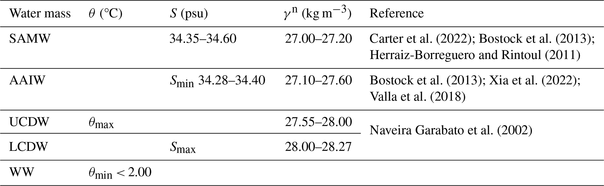
Note: SAMW, Subantarctic Mode Water; AAIW, Antarctic Intermediate Water; UCDW, Upper Circumpolar Deep Water; LCDW, Lower Circumpolar Deep Water; WW, Winter Water.

Between the SAF and NB, well-defined layers of SAMW, AAIW, and Upper Circumpolar Deep Water (UCDW) are observed from the upper to lower layer in the AE (Fig. 9d, j), confirming their local origin within the Antarctic Convergence Zone. Conversely, the CE in the same zone shows markedly different θ–S structure (Fig. 9a, g), with upper layers (< 1000 dbar) lacking SAMW/AAIW signatures and instead containing colder, fresher waters of southern origin. Neutral density (γⁿ) surfaces in the CE are approximately 200 dbar shallower than in the AE, demonstrating that CEs effectively transport high-potential-energy southern waters into the SAF-NB zone. This establishes strong mesoscale potential energy contrasts between the low-potential-energy waters in AEs and the high-potential-energy waters in CEs, an energetic precondition for baroclinic instability via the release of available potential energy (Fu et al., 2023).

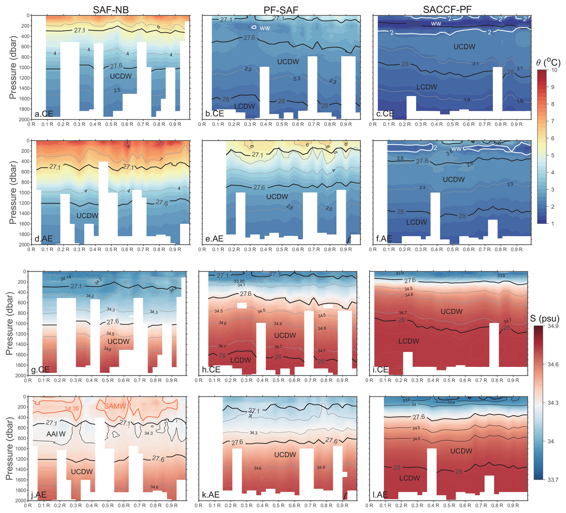
Figure 9 Sectional distributions of θ (a–f) and S (g–l) along normalized eddy radius (R) direction in the interfrontal zones of SAF-NB (the left panels), PF-SAF (the middle panels), and SACCF-PF (the right panels). Black thick contours indicate neutral density (γⁿ, kg m⁻³), thin contours represent θ or S isolines, respectively.

In the PF-SAF region, both the CE and AE maintain thermohaline contrasts similar to those in the SAF-NB zone but with reduced magnitude, preserving the characteristic warmer/saltier AE and colder/fresher CE signatures (the middle panels of Fig. 9). Notably, only the CE's upper layer exhibits distinct Winter Water (WW) characteristics, confirming their southern origins. Below this, the normalized CE sequentially displays UCDW and LCDW, while the AE shows only UCDW beneath the relatively warm and salty Antarctic Surface Water within the upper 2000 dbar. The vertical isopycnal structure reveals depth-dependent displacements: in the near-surface layer, the CE's isopycnal γⁿ=27.1 kg m⁻³ is ∼ 100 dbar shallower than the AE, while at intermediate depths, the CE's isopycnal γⁿ=27.6 kg m⁻³ (400–600 dbar) is ∼ 500 dbar shallower than the AE (∼ 1000 dbar).

The thermohaline anomalies between CE and AE still exist in the SACCF-PF zone (the right panels of Fig. 9). In the CE, a subsurface WW layer overlies a warm UCDW core, with LCDW dominating below 1000 dbar, showing a characteristic of waters south of the SACCF (Aoki et al., 2013; Auger et al., 2021). While the AE also contains these water masses, they show weaker WW expression, a more pronounced θ_max core, and vertically extended UCDW, reflecting their relatively northern origins. Isopycnals in the CE remain consistently 300–400 dbar shallower than in the AE throughout the water column.

Therefore, the normalized AE and CE possess distinct water mass distributions within the same inter-frontal zones, marked by profound isopycnal thermohaline differences. AEs and CEs transport their respective source water masses into the same zones, amplifying mesoscale hydrographic variability. The above comparative analysis demonstrates that cross-frontal CEs play a dominant role in meridional water mass transport, particularly in the SAF-NB and SACCF-PF zones, consistent with their greater dynamical vigor. This cross-frontal exchange reduces baroclinicity between interfrontal zones while enhancing mesoscale available potential energy within individual zones.

4 Discussion

This study reveals a fundamental polarity- and direction-dependent asymmetry in cross-frontal eddy (CFE) dynamics within the Pacific sector of the SO. This asymmetry manifests in three key aspects: (1) a distinct abundance hierarchy among CFE types, (2) contrasting EKE intensities and trends, and (3) polarity- and direction-selective energy transfers during eddy-frontal jet interactions. The observed hierarchy, in which CEs predominantly migrate equatorward and AEs poleward, aligns with established eddy dynamics in the SO (He et al., 2023; Li et al., 2022a; Patel et al., 2019). Beyond abundance, the dominant types (equatorward CEs and poleward AEs) exhibit superior energetic characteristics, including higher EKE levels (Fig. 4f), longer propagation distances (Fig. 3), and stronger nonlinearity compared to their counterparts. Our results demonstrate that substantial energy gain during frontal crossing sustains the enhanced energetics of these two dominant complete CFE types, as illustrated in Fig. 11. Moreover, the energy compensation relationships (Fig. 5i, j) suggest that partial and transient CFEs of the same dominant polarity-direction combinations likely follow a similar energization mechanism. Taken together, these findings indicate that polarity- and direction-dependent eddy-front interactions fundamentally govern CFE energetics and, consequently, their capacity to drive meridional heat and material transport across Southern Ocean frontal zones.

Although CFE abundance shows no significant trend over 2000–2022, both polarity groups experienced substantial EKE_T intensification, with CEs gaining energy at (2.27 ± 1.45) × 10⁶ m⁴ s⁻² yr⁻¹ (excluding the anomalously low 2017 value) and AEs at (2.27 ± 0.94) × 10⁶ m⁴ s⁻² yr⁻¹. The increasing trends are also robust in terms of annual area-weighted mean EKE (EKE = EKE${}_{\mathrm{T}}/S$, where S is the total area of an eddy; Fig. S1 in the Supplement), with trends of 3.71 ± 2.08 cm² s⁻² yr⁻¹ for CEs and 2.58 ± 0.97 cm² s⁻² yr⁻¹ for AEs. The EKE enhancements are even more pronounced for the dominant subsets, equatorward CEs and poleward AEs (Figs. 4, S1). These rates substantially exceed previously reported EKE trends. Hogg et al. (2015) estimated a regional mean EKE increase of 14.9 ± 4.1 cm² s⁻² per decade under intensifying westerlies in the Pacific sector (1990–2015). Similarly, Zhang et al. (2021) documented an EKE increase of < 20 cm² s⁻² per decade south of New Zealand and downstream of the Campbell Plateau, identified as the only region with significant EKE rise in the SO during 1993–2018. The EKE trends for CFEs presented here are considerably larger than these basin-scale estimates. In contrast, non-CFEs exhibit lower EKE levels and no comparable EKE_T increase (Fig. 10). The significant area-weighted mean EKE trend for non-frontal crossing CEs is also weaker (Fig. S2). These contrasts suggest that the overall EKE increase in the Pacific sector is primarily attributable to CFEs. Non-CFEs contribute little to, or may even obscure, the observed EKE trends. This finding implies that eddy-front interactions, rather than basin-scale wind forcing alone, may be the primary driver of recent EKE trends in the Pacific sector of the SO.

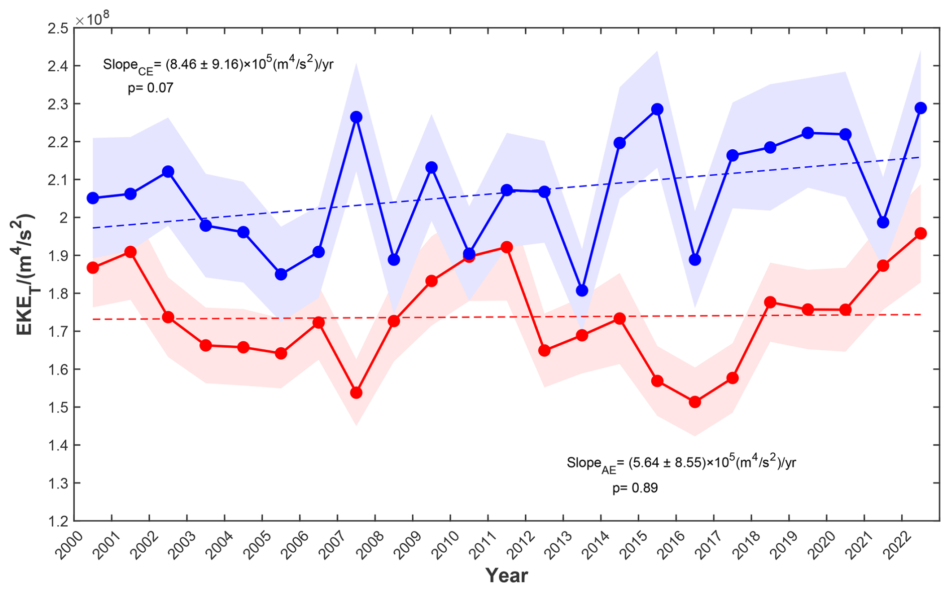
Figure 10 Time series of annual mean EKE_T for eddies in the interfrontal zones. EKE_T is shown by blue solid line for CEs and red solid line for AEs, with linear regression indicated by dashed lines, error shadings representing one standard deviation, and slope values given with ±95 % confidence intervals.

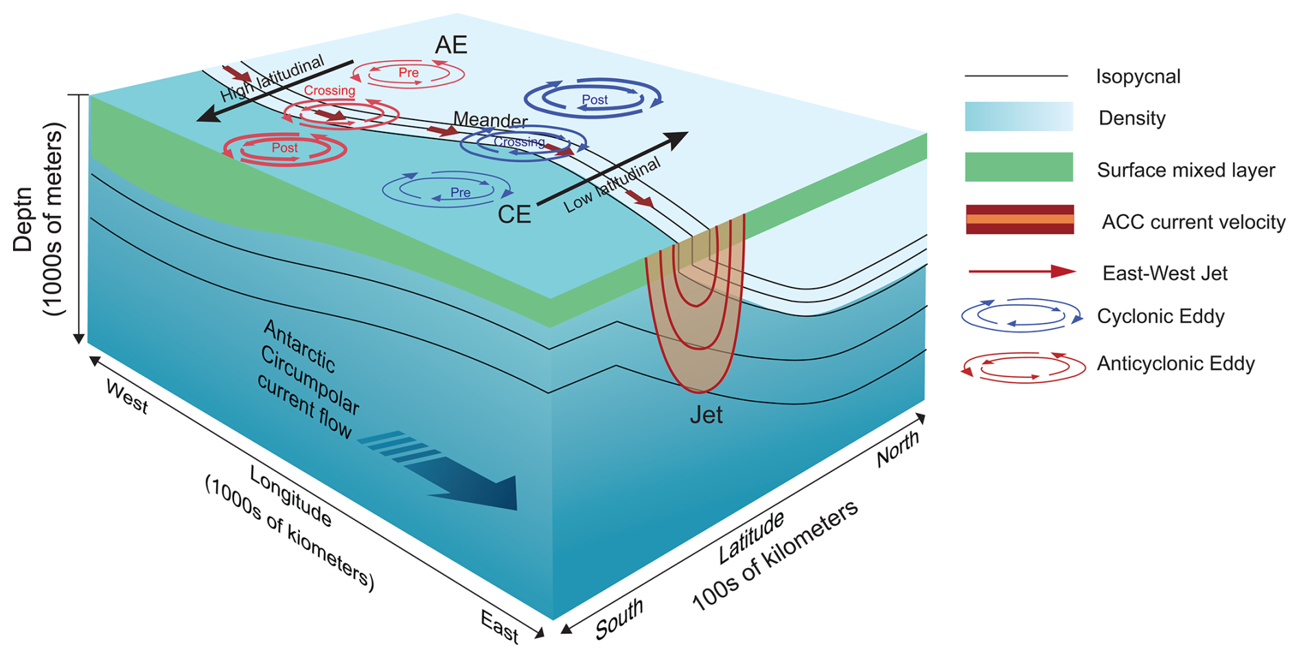
Figure 11 Illustrations of EKE variations during frontal crossing for poleward AEs and equatorward CEs (modified from Fig. 1 in Chapman et al., 2020). The thickness of rotational velocity vectors represents relative flow intensity.

Our results suggest that the enhanced wind stress (Hogg et al., 2015; Menna et al., 2020) could preferentially energize cross-frontal activity, especially the CFEs achieving complete frontal crossing (Fig. 5). The predominance of equatorward CEs aligns with intensified Ekman transport patterns reported by Shi et al. (2025), also suggesting wind-driven facilitation of meridional eddy migration. Building on Fu et al.'s (2023) framework of wind-driven energy pathways (baroclinic: mean kinetic energy → mean available potential energy → mesoscale available potential energy → EKE; barotropic: mean kinetic energy → EKE), we found that only equatorward CEs and poleward AEs gain kinetic energy from frontal jets (Table 2; Figs. 6, 7). This energization likely arises from two synergistic mechanisms: (1) barotropic instability from enhanced horizontal shear when eddy rotation aligns with the eastward jet (Qiu et al., 2024), and (2) baroclinic instability triggered by potential energy release for enhanced hydrographic gradients with ambient waters (Fu et al., 2023). Conversely, significant energy losses of poleward CEs and equatorward AEs during frontal crossing, possibly due to counter-rotational turbulent dissipation (Dong et al., 2017; Jan et al., 2017) and upwelling (downwelling)-induced baroclinicity reduction with the ambient waters.

Intensifying and poleward-shifting westerlies have emerged as a dominant dynamic forcing mechanism in the SO (Behrens and Bostock, 2023; Hogg et al., 2015). Meanwhile, buoyancy forcing from meridionally inhomogeneous ocean warming has been shown to accelerate the ACC at 48° S–58° S (Shi et al., 2021). Our results demonstrate that CFEs play a vital role in mediating the oceanic response to these forcings by compensating for heat transport (Fig. 9). By facilitating equatorward cold-water transport via CEs and poleward warm-water transport via AEs, CFEs reduce cross-frontal water mass property gradients. This process effectively buffers wind- or warming-induced increases in baroclinicity. thereby maintaining the SO's thermal equilibrium and modulating the ACC's response to external forcing. These findings highlight the dual role of CFEs as both energy transporters and dynamical stabilizers in a changing climate.

This study has several limitations that should be noted. First, the analysis does not account for potential interannual or seasonal variations in frontal positions. However, a comprehensive sensitivity analysis, in which the frontal zone half-width was expanded to $\pm (\mathrm{25}+R)$ km, confirms that all key conclusions remain qualitatively and statistically robust (see Supplement, Tables S1 and S2, and Figs. S3–S6). Second, the hydrographic analysis utilized all qualified Argo profiles from 2000 to 2022 without segregating interannual or seasonal variability, which may introduce some uncertainty into the normalized water mass properties. Finally, while this study focuses on eddy characteristics, it does not evaluate the dynamic properties of the frontal jets themselves. A detailed analysis of jet variability and energy transfer is essential for a more comprehensive mechanistic understanding of eddy-jet interactions and represents an important direction for future research.

5 Conclusions

This study provides a comprehensive characterization of cross-frontal eddies (CFEs) in the Pacific sector of the Southern Ocean, revealing fundamental asymmetries that govern their role in meridional transport and energy exchange. Through the integration of multi-decadal satellite altimetry and in-situ hydrographic data, we have demonstrated that CFE activity is not random but follows a well-defined polarity- and direction-dependent hierarchy. The predominance of equatorward-moving cyclonic eddies (CEs) and poleward-moving anticyclonic eddies (AEs) reflects an intrinsic organization in cross-frontal exchange pathways that has profound implications for Southern Ocean dynamics.

Three key findings emerge from our analysis. First, the observed CFE abundance hierarchy is complemented by significant differences in energetic characteristics, with the dominant types (equatorward CEs and poleward AEs) exhibiting superior kinetic energy levels, longer propagation distances, and stronger nonlinearity. Second, these eddies experience sustained energization through polarity-selective energy transfers during frontal crossings, gaining kinetic energy from the eastward frontal jets while their counterparts experience energy dissipation. The intensification of CFE activity has occurred over the past two decades, with EKE trends substantially exceeding previous basin-scale estimates, suggesting that eddy-front interactions, rather than wind forcing alone, drive recent energetic changes in the region. Third, hydrographic analyses confirm that CFEs function as effective transporters of distinct water masses, with CEs and AEs maintaining sharp thermohaline contrasts within the same interfrontal zones. This cross-frontal exchange reduces large-scale baroclinicity while enhancing mesoscale available potential energy, creating a dynamic balance that regulates meridional heat transport.

As climate change intensifies westerly winds and modifies buoyancy forcing, CFEs are likely to play an increasingly important role in modulating the ACC's response to external forcing. Their ability to maintain thermal equilibrium across frontal zones highlights their significance for understanding future changes in Southern Ocean circulation, carbon uptake, and global climate feedbacks. Future research should focus on quantifying the precise contribution of CFEs to meridional heat and carbon fluxes and investigating how their stabilizing role might evolve under continued climate change.