Passive acoustic monitoring from profiling floats as a pathway to scalable autonomous observations of global surface wind

Wind forcing plays a pivotal role in driving upper-ocean physical and biogeochemical processes, yet direct wind observations remain sparse in many regions of the global ocean. While passive acoustics have been used to estimate wind speed from moored and mobile platforms, their application to profiling floats has been demonstrated only in limited cases. Here we report the first deployment of a biogeochemical profiling float equipped with a passive acoustic sensor explicitly designed for wind retrieval, aimed at detecting wind-driven surface signals from depth. The float was deployed in the northwestern Mediterranean Sea near the DYFAMED (DYnamique des Flux Atmosphériques en MEDiterranée) meteorological buoy from February to April 2025 and operated at parking depths of 500–1000 m. We demonstrate that wind speed can be successfully retrieved from subsurface ambient noise using established acoustic algorithms, with float-derived estimates showing good agreement with collocated surface observations. To evaluate scalability to remote regions, we simulate a remote deployment scenario by refitting the acoustic model of Nystuen et al. (2015) using ERA5 reanalysis as a reference for surface wind. The ERA5-based calibration performs well under moderate winds but exhibits systematic high-wind bias (≥ 10 m s⁻¹). Finally, we apply a residual learning framework to correct these estimates using a limited subset of DYFAMED wind data, simulating conditions where only brief surface observations are available. The corrected wind time series achieved a 38.6 % reduction in RMSE, demonstrating the effectiveness of combining reanalysis with sparse in-situ calibration. This framework improves agreement with in-situ wind observations relative to reanalysis alone, supporting a scalable strategy for float-based wind monitoring in data-sparse ocean regions. Such capability has direct implications for improving estimates of air–sea exchanges, interpreting biogeochemical fluxes, and advancing climate-relevant ocean observing.

1 Introduction

Wind plays a fundamental role in driving ocean circulation, mediating air–sea gas exchange, and shaping climate-related biogeochemical processes (Wanninkhof, 2014; McGillicuddy, 2016). Recent studies show that wind-driven circulation strongly influences regional climate trends (eg., Pellichero et al., 2020; Trenberth et al., 2025; McMonigal et al., 2025). Despite its central importance, accurately quantifying wind variability in remote ocean basins remains challenging. Satellite scatterometers suffer from coarse resolution, reduced performance under extreme weather and heavy cloud cover, and signal degradation in high-latitude regions, while surface moorings provide limited spatial coverage (Bentamy et al., 2003; Chelton et al., 2007; Stoffelen et al., 2008).

Passive acoustic monitoring of underwater ambient noise offers a complementary approach for inferring surface meteorological conditions from surface-generated underwater noise. The relationship between wind speed and high-frequency (1–20 kHz) noise generated by wave breaking and bubble entrainment has been extensively documented (Vagle et al., 1990; Farmer et al., 1998; Oguz and Prosperetti, 1990). This principle underpins the Weather Observations Through Ambient Noise (WOTAN) techniques and the development of Passive Acoustic Listener (PAL) instruments (Nystuen, 2001), enabling autonomous, long-term estimates of wind and rainfall from fixed and drifting platforms.

Although widely used, these approaches still face several limitations. The empirical relationships underpinning WOTAN-type methods are often site dependent, with deviations arising from bathymetry, wave regime, and water depth; even under wind-dominated conditions, shallow-water environments can yield substantially different spectral levels (Ingenito, 1987). Model skill is also limited by model design, as single-regime formulations underestimate the slope at higher winds and bias comparisons across SPL–wind relationships (Schwock and Abadi, 2021). These factors complicate the selection of an appropriate empirical law for a given platform or region. To address these challenges, recent studies have explored data-driven and machine-learning approaches that learn wind–noise relationships directly from observations and reduce reliance on fixed empirical models (Taylor et al., 2020; Trucco et al., 2023; Zambra et al., 2023).

Despite these limitations, the WOTAN framework has proven applicable across a wide range of platforms. Wind-driven signatures have been detected from moorings (Ma and Nystuen, 2005; Nystuen et al., 2015; Pensieri et al., 2015), gliders (Cauchy et al., 2018; Cazau et al., 2019) and profiling floats (Riser et al., 2008; Yang et al., 2015; Yang et al., 2016; Bytheway et al., 2023; Ma et al., 2023), and even from biologged marine mammals operating in remote regions (Menze et al., 2013; Cazau et al., 2017; Gros-Martial et al., 2025a). Beyond wind estimation, acoustic sensors integrated into autonomous platforms have supported a wide range of geophysical and ecological applications, including marine mammal monitoring (Matsumoto et al., 2013; Cauchy et al., 2020; Fregosi et al., 2020; Baumgartner and Bonnel, 2022), and hydroacoustic earthquake detection and characterisation of ambient ocean noise (Baumgartner et al., 2017; Pipatprathanporn and Simons, 2022).

Recognising this broad utility, the Ocean Sound Essential Ocean Variable (EOV), coordinated by the International Quiet Ocean Experiment (IQOE) and endorsed by the Global Ocean Observing System (GOOS), identifies autonomous platforms such as profiling floats as ideal platforms for distributed global acoustic monitoring (Tyack et al., 2023). In recent decades, biogeochemical (BGC)-Argo floats have become a central component of global ocean observing systems. Their persistence at sea, broad spatial coverage, and cost-effectiveness have demonstrated clear advantages over traditional ship-based measurements (Roemmich et al., 2009; Riser et al., 2016). As their capabilities have expanded, these platforms now host increasingly sophisticated multidisciplinary sensor suites, with measurements of oxygen, nitrate, chlorophyll, pH, and irradiance (Johnson and Claustre, 2016; Claustre et al., 2020; D’Ortenzio et al., 2020). Yet, despite this progress, the integration of passive acoustics into BGC-Argo remains largely unexplored. Incorporating acoustic wind sensing would supply the atmospheric forcing needed to interpret biogeochemical variability, particularly in high-latitude or storm-dominated regions where wind products remain sparse or uncertain.

Here, we present the first deployment of a biogeochemical profiling float equipped with a passive acoustic sensor explicitly designed for wind speed estimation from underwater ambient noise. Deployed in the northwestern Mediterranean Sea, near the DYFAMED (DYnamique des Flux Atmosphériques en MEDiterranée) meteorological buoy, this float serves as a proof-of-concept demonstration to: (1) determine whether wind-driven acoustic signatures can be detected at profiling float parking depths; (2) evaluate the performance of established acoustic wind models on this platform; and (3) develop a practical framework combining acoustic observations with reanalysis data and machine learning to enable wind estimation in remote regions. Through this approach, we demonstrate the potential of acoustic-equipped profiling floats to expand global wind observations, close persistent observational gaps, and support interpretation of biogeochemical and climate-relevant processes.

2 Materials and Methods

2.1 Study area and DYFAMED weather station

The acoustic wind sensing trial was conducted in the Ligurian Sea, a sub-basin of the northwestern Mediterranean, in proximity to the DYFAMED (DYnamique des Flux Atmosphériques en MEDiterranée) oceanographic time series station (Fig. 1). This station is part of the national observation program MOOSE (Mediterranean Ocean Observing System for the Environment, https://www.moose-network.fr, last access: 28 May 2025), funded by CNRS–INSU, and has been integrated since 2016 into the national research infrastructure ILICO (Infrastructure de recherche littorale et côtière; Cocquempot et al., 2019).

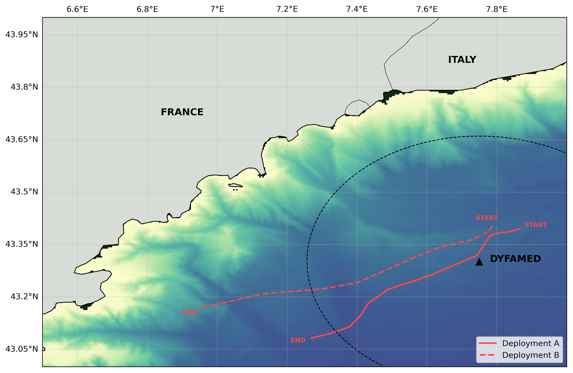
Figure 1 Float trajectories during sea trials conducted in the Ligurian Sea in February and March 2025. Deployment A (solid line) and Deployment B (dashed line) are shown along with a concentric dashed circle (40 km radius) centred on the DYFAMED station. The 40 km radius was used to spatially filter float data for refitting and validation of wind estimates at DYFAMED, as described in Cauchy et al. (2018).

Located at 43.42° N, 7.87° E, DYFAMED has served as a key reference site for air–sea exchange, upper ocean dynamics, and biogeochemical cycling since the early 1990s. The site is equipped with continuous meteorological and oceanographic monitoring, including high-quality wind speed and direction measurements from the Côte d'Azur meteorological buoy operated by Météo-France, located at the DYFAMED site. These data are reported at hourly resolution following WMO (World Meteorological Organization) standards and include wind parameters, air temperature, pressure, humidity, and sea state.

During the study period, wind speeds at DYFAMED ranged from 0.5 to 16.1 m s⁻¹, with a mean of 6.8 m s⁻¹ and a measurement precision of one decimal place.

2.2 Acoustic sensor integration

The float used in this study was equipped with a passive acoustic module jointly developed by NKE and ABYSsens in collaboration with LOV. This module was specifically designed for integration into the PROVOR CTS5 BGC-Argo platform, with the aim of minimizing power consumption and data volume while remaining compatible with the operational constraints of the BGC-Argo program.

The module consists of two main parts enclosed in a dedicated external housing: (1) a low-noise HTI-96-Min hydrophone (sensitivity: −165 dB re 1 V µPa⁻¹; frequency range: 2 Hz–30 kHz), mounted externally to capture pressure fluctuations, and (2) an ABYSsens acquisition board, which conditions, digitizes, and processes the signal.

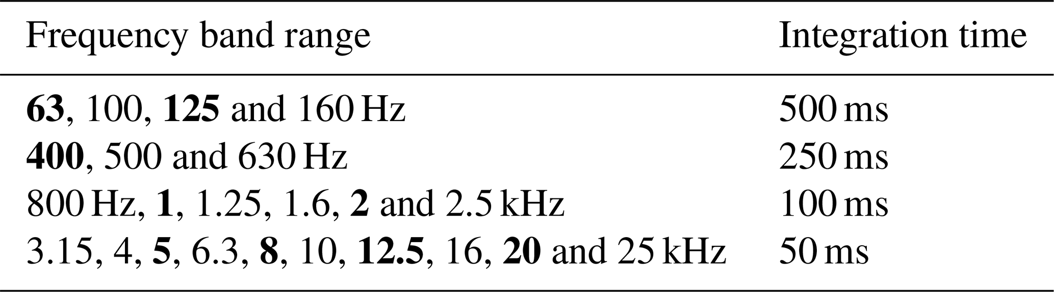
The acquisition system operates in a low-power pulsed mode (220 mW) with a sampling frequency up to 62.5 kHz and 24-bit resolution. To limit power usage and transmission needs, raw acoustic signals are not stored. Instead, the sensor performs direct onboard integration into 23 third-octave bands, spanning from 63 Hz to 25 kHz with a variable integration time (see Table 1). Higher-frequency bands (e.g., 3.15–25 kHz) used shorter integration times (50 ms), while low-frequency bands used longer windows (up to 500 ms).

Table 1 Integration times applied to third-octave bands during acoustic signal processing, varying by frequency range to balance energy and spectral accuracy. In bold, the bands transmitted in the 9-band float configuration.

The acoustic unit is mounted on the upper section of the float chassis and is configured to operate exclusively during the parking phase (500–1000 m depth; Fig. 3). During this phase, the float drifts with only routine background measurements (e.g., pressure, CTD), and acoustic acquisition is automatically suspended whenever noisy operations such as ballast pumping or CTD sampling occur, thereby avoiding contamination from self-noise.

The float system allows for flexible and modifiable configuration via satellite: the user can define the number of bands transmitted (23, 9, or a compact onboard estimate of wind/rain), the acquisition interval (typically 5–15 min), and the number of acoustic samples averaged per measurement. In this study, we used a 5 min interval with 10 averaged acquisitions per measurement (each acquisition is a spectral estimation using the integration times defined in Table 1).

The telemetry and energy impact of adding an acoustic sensor to a 6-variable biogeochemical float was evaluated by using the programming interface provided by NKE. The estimated reduction in the number of cycles varies from 18 % for acquisition every 5 min to 7 % for acquisition every 15 min during the whole parking drift of a 10 d Argo cycle and with 5 averaged acquisitions per acoustic measurement. The data volume increase depends on the transmission format: from ∼ 9 % for onboard wind–rain estimates (15 min period) to ∼ 85 % for a full 23-band spectrum (5 min period). A 9-band spectrum every 15 min – a likely recommended setup – adds ∼ 16 %. These overheads remain within the platform's capacity, confirming compatibility with concurrent BGC measurements.

Each sensor output transmitted by the float corresponds to the Third Octave Level (TOL), i.e., the sound pressure level integrated over a third-octave band, expressed in dB re 1 µPa. These TOLs represent the float's primary spectral product and are used as input to the wind speed retrieval models. The amplitude resolution of the transmitted data is 0.2 or 0.5 dB, with a dynamic range up to 127 dB. This discretisation arises because the data are transmitted as integers to save bandwidth, which requires selecting a resolution step.

2.3 Depth correction and spectral normalization

To account for the attenuation of surface-generated noise with depth, a correction term β(h,f) was applied to all acoustic measurements (Fig. 2). Because β depends on the ambient temperature–salinity structure, we quantified hydrographic stability over the 60 d deployment using all profiles that reached at least 1000 dbar. Each profile was interpolated onto a 1 m grid and compared to the deployment-mean temperature/salinity profiles. Depth-averaged RMS deviations were 0.14 ± 0.04 °C for temperature and 0.06 ± 0.02 for salinity, and no profile exceeded $|z=\mathrm{2}$ standardised deviation, confirming weak hydrographic variability. Because such differences are far below hydrophone measurement uncertainties, β(h,f) was computed once using the deployment-mean profile and applied uniformly to the full record. For longer or more dynamic missions, β(h,f) should be recomputed for each profile. Modern hardware makes this operation computationally inexpensive, but the negligible hydrographic variability in this deployment renders repeated recalculation unnecessary.

Following Cauchy et al. (2018), the correction takes the form:

$$\begin{array}{}\text{(1a)}& {\displaystyle }{\mathrm{TOL}}_{\mathrm{0}}\left(f\right)=\mathrm{TOL}(h,f)+\mathit{\beta }(h,f),\text{(1b)}& {\displaystyle }\begin{array}{rl}\text{where}& \mathit{\beta }\left(h,f\right)=\\ & -\mathrm{10}\log \left\{\mathrm{2}\underset{\mathrm{0}}{\overset{\mathrm{\infty }}{\int }}\left[{\displaystyle \frac{r{\sin }^{\mathrm{2}}{\mathit{\theta }}_{r,h}{e}^{-{\mathit{\alpha }}_f{l}_{r,h}}}{l_{r,h}^{\mathrm{2}}}}\right]\mathrm{d}r\right\},\end{array}\end{array}$$

with TOL(h, f) as the raw TOL measurement from the profiling float, h as the sensor depth, f the centre frequency of the band, r the horizontal distance from a surface noise source to the point vertically above the sensor, l the total pathlength between source and receiver (accounting for depth and refraction), including refraction effects, θ the angle between the emitted acoustic ray and the horizontal axis, and α the frequency-dependent attenuation coefficient for bubble-free water. The integral considers contributions from all surface-generated acoustic sources over the sea surface, assuming radial symmetry, and accounts for geometric spreading, frequency-dependent absorption, and angle-dependent energy emission along each path. This correction was originally derived for third-octave levels and is directly applicable here, as the float outputs TOLs at fixed centre frequencies. Then, depth-corrected third-octave levels TOL₀(f) (dB re 1 µPa) were converted to spectral density levels SPL(f) (dB re 1 µPa Hz⁻¹) by normalising to the bandwidth of each band. In the following, SPL always refers to these depth-corrected, bandwidth-normalised values derived from TOL₀(f). This step ensures consistency across frequencies and comparability with model spectra. In future deployments, this spectral correction will be applied directly onboard the float.

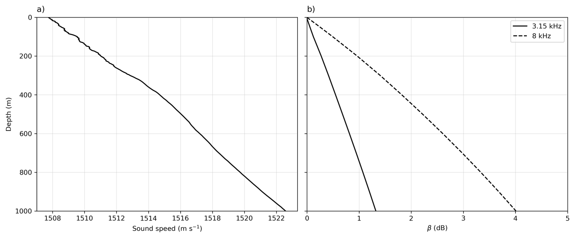
Figure 2 (a) Mean sound-speed profile derived from the deployment-average temperature and salinity, and used to compute (b) the depth-correction term β(h,f) following Cauchy et al. (2018). The correction accounts for the attenuation of wind-generated surface noise with increasing hydrophone depth and was applied prior to wind-speed retrieval. β is shown here for 3.15 and 8 kHz.

2.4 Profiling float deployments

Two deployments of an acoustic-equipped float (PROVOR CTS5) were carried out near DYFAMED between February and April 2025 (Fig. 1). Deployment A lasted 30 d, from 10 February to 11 March, and Deployment B continued for 24 d starting on 12 March and remained active until 4 April. The float operated in park-and-profile mode at three parking depths (500, 700, and 1000 m; Fig. 2), collecting biogeochemical data during ascent and passive acoustic data exclusively during the parking phases to minimize self-generated noise.

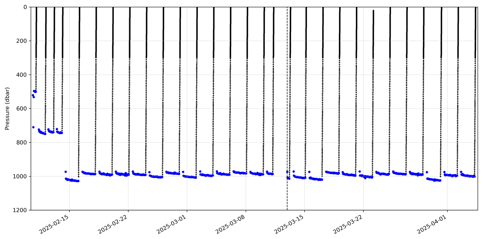
Figure 3 Vertical profiles from the acoustic-equipped profiling float deployed near DYFAMED between February and April 2025. Blue points indicate times when passive acoustic data were successfully recorded. The vertical dashed line marks the transition between Deployment A and Deployment B.

While Riser et al. (2008) previously demonstrated the feasibility of acoustic wind sensing from Argo floats, their system transmitted only pre-processed wind estimates derived onboard using a simplified version of the algorithm by Nystuen et al. (2015), without retaining or transmitting spectral band data. This limited the possibility of reanalysis or applying alternative processing schemes. In contrast, the floats used in this study recorded and transmitted full third-octave band spectra, enabling detailed post-processing and algorithm refinement tailored to the float's specific acoustic characteristics.

2.5 Transient and anthropogenic noise mitigation

Transient noise (i.e., episodic non-wind-related events) was mitigated by removing values exceeding the 99th percentile within a ±1.5 h window centred around each matched timestamp. This percentile corresponds to discarding roughly the top 1 % of samples over a 3 h window (≈2 min of data). No physically meaningful wind- or wave-driven variability relevant to this study evolves on such short timescales, making this filter effective at removing brief acoustic artefacts without suppressing real high-wind conditions. This approach is conceptually similar to the transient-noise mitigation used in glider-based PAM studies (e.g., Cauchy et al., 2018), which suppress short-lived spikes in the spectra to isolate wind-generated noise.

To further reduce short-term variability and emphasize quasi-stationary wind-driven acoustic patterns, we applied a 3 h rolling mean to each frequency band. This smoothing window is conceptually consistent with the profile-scale averaging used in glider-based acoustic wind studies (e.g., Cauchy et al., 2018), where acoustic measurements are aggregated over ∼ 2 h glider dives to suppress transient variability. While smoothing inevitably attenuates rapid fluctuations, the 3 h window stabilises the spectra without erasing multi-hour wind events relevant for air–sea flux applications. Alternative strategies, such as post-processing the wind speed estimates rather than the spectral bands, could be explored in future deployments if finer-scale variability is a priority.

Anthropogenic noise was mitigated using AIS vessel tracks. Because the float only provides GPS positions at the surface, we reconstructed a continuous trajectory by linearly interpolating its positions between successive surfacings at hourly resolution. Each 5 min acoustic record was then associated with the nearest interpolated position. An observation was flagged as potentially contaminated when an AIS-reported vessel was located within 20 km of this interpolated float position and within ±30 min of the acoustic timestamp. The 20 km radius corresponds to the distance over which ship-radiated noise commonly dominates the ambient sound field in the 1–10 kHz band under low-to-moderate sea states, while the ±30 min window accounts for the typically irregular AIS reporting interval offshore. As an additional safeguard, we excluded cases where the float-derived wind speed deviated from the DYFAMED buoy by more than the RMSE computed under uncontaminated conditions. This RMSE criterion is used only as a secondary check to capture possible contamination during periods of poor AIS coverage. Sensitivity tests indicate that moderate changes to these thresholds do not affect the main conclusions.

2.6 Application of established acoustic models

Empirical models have long been used to estimate surface wind speed from underwater ambient noise, exploiting the link between wind-driven bubble formation and acoustic energy in the 1–20 kHz band. These models typically relate surface wind speed U to the sound pressure level L_f measured in selected frequency bands. While many models use third-octave bands, others rely on custom-defined or narrowband frequencies, often with variable bandwidths (e.g., 16 % of the centre frequency in Vagle et al., 1990).

Table 2 Summary of acoustic wind speed estimation models and their input requirements. Input units refer to the spectral level units used in model calibration. Central frequency indicates the nominal retrieval frequency, and the third-octave band column specifies the corresponding bandwidth. All models were calibrated and validated against standard 10 m wind speed.

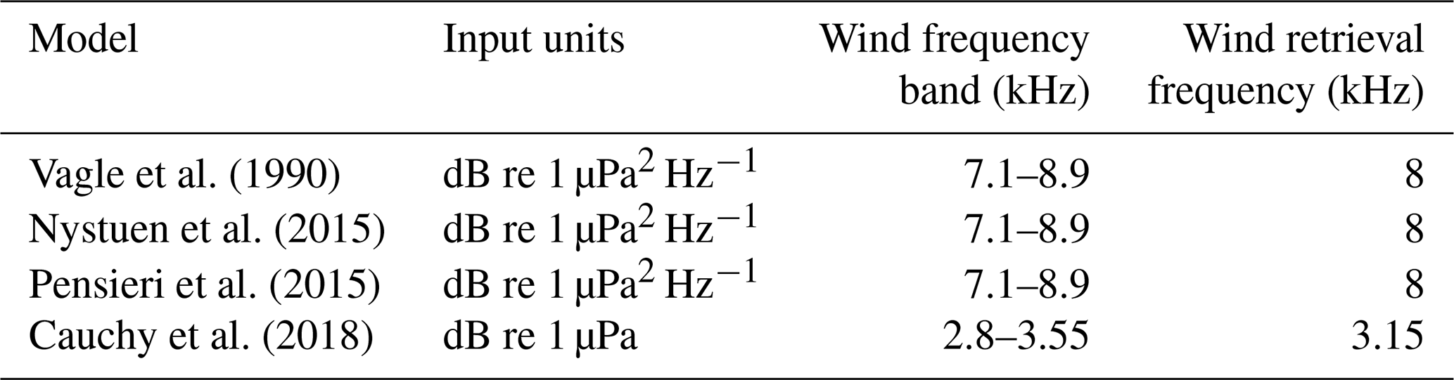
We applied four established wind retrieval models spanning a range of functional forms – cubic, two-regime linear–quadratic, composite, and two-regime log–linear. All wind models were applied using acoustic levels consistent with their original formulations (Table 2). This diversity allowed us to assess sensitivity to model structure and evaluate performance under float-specific conditions. Each model was first implemented using its published coefficients to generate wind speed estimates from float acoustic data, and the results were evaluated against collocated meteorological observations (Fig. 4). Subsequently, the parameters of each model were refitted using collocated float acoustic and wind data from the DYFAMED meteorological buoy (Figs. 4 and 5), which provides hourly 10 m wind speed. Model refitting was performed using nonlinear least-squares optimization (Table 3). Wind records from DYFAMED were matched to float measurements by nearest timestamp.

Following the spatial filtering approach of Cauchy et al. (2018), only float data within 40 km of DYFAMED were retained for refitting and validation (Fig. 1). This threshold corresponds to the estimated confidence radius around the DYFAMED meteorological buoy, within which wind speed measurements show high spatial coherence (R = 0.86, RMSE = 2.5 m s⁻¹) when compared to the AROME-WMED atmospheric model (Rainaud et al., 2014). Although originally derived from the spatial wind-field decorrelation scale reported by Cauchy et al. (2018), this 40 km radius reflects a regional mesoscale atmospheric property rather than a platform-specific constraint. Because our deployment occurred in the same NW Mediterranean basin, this decorrelation length remains appropriate for our case. We note, however, that this threshold is region-dependent and should be re-evaluated for future deployments elsewhere.

The updated coefficients were then used to generate wind estimates over the full float dataset. While this spatial proximity improves wind representativeness, it does not account for variations in wind fetch, a parameter known to influence ambient noise generation, particularly through wave and bubble field development (e.g., Prawirasasra et al., 2024).

These four models were selected to represent a range of analytical formulations commonly used in acoustic wind retrievals. They all use frequency bands where wind-driven bubble noise typically dominates the local ambient sound field, with reduced interference from low-frequency sources such as distant shipping. Our aim was not to exhaust all available models, but rather to evaluate a representative subset under consistent float-specific conditions, emphasizing the effect of model structure and local fitting.

The specifications and key features of each model are summarized in Table 2 for reference. For all models and validation steps throughout the rest of Methods section, wind speed refers to the standard 10 m wind speed, consistent with both the ERA5 reanalysis product and the DYFAMED buoy observations used for calibration and evaluation.

The first model, from Vagle et al. (1990), was derived from moored hydrophone data in the North Atlantic and relates wind speed to high-frequency noise at 8 kHz using a cubic formulation:

$$\begin{array}{}\text{(2)}& U_{\mathrm{Vagle}\mathrm{1990}}={\mathrm{10}}^{\left(\frac{-\mathrm{38.70}+\sqrt{-{\mathrm{38.70}}^{\mathrm{2}}-\mathrm{4.7}\cdot \mathrm{38}\cdot ({\mathrm{SPL}}_{\mathrm{8}\mathrm{kHz}}-\mathrm{21.69})}}{-\mathrm{7.38}\cdot \mathrm{2}}\right)}.\end{array}$$

Next, we applied the cubic model from Nystuen et al. (2015), developed using long-term acoustic records from fixed hydrophones in both the Pacific and Atlantic. This model targets wind-generated noise at 8 kHz and includes band-specific criteria to distinguish wind contributions from other sources such as rain and shipping (Table 2).

$$\begin{array}{}\text{(3)}& \begin{array}{rl}{U}_{\mathrm{Nystuen}\mathrm{2015}}& =\mathrm{0.0005}\cdot {\mathrm{SPL}}_{\mathrm{8}\mathrm{kHz}}^{\mathrm{3}}-\mathrm{0.0310}\cdot {\mathrm{SPL}}_{\mathrm{8}\mathrm{kHz}}^{\mathrm{2}}\\ & +\mathrm{0.4904}\cdot {\mathrm{SPL}}_{\mathrm{8}\mathrm{kHz}}+\mathrm{2.0871}\end{array}\end{array}$$

We then tested the two-regime linear–quadratic model from Pensieri et al. (2015) at 8 kHz, developed using moored hydrophone data from the Ligurian Sea, near our study area. Calibrated for Mediterranean conditions, the model relates wind speed to ambient noise levels at the 8 kHz band, applying distinct linear and quadratic fits across low- and high-noise regimes. Notably, the transition between regimes is defined at 38 dB, corresponding to a wind speed of 2.39 m s⁻¹ in their framework. However, it is important to note that the threshold separating high and low regimes is not standardized across the literature and may vary between studies.

$$\begin{array}{}\text{(4)}& \begin{array}{rl}& U_{\mathrm{Pensieri}\mathrm{2015}}=\\ & \left\{\begin{array}{c}\mathrm{0.044642}\cdot {\mathrm{SPL}}_{\mathrm{8}\mathrm{kHz}}^{\mathrm{2}}-\mathrm{3.2917}\cdot {\mathrm{SPL}}_{\mathrm{8}\mathrm{kHz}}+\mathrm{63.016}\\ \mathrm{0.1458}\cdot {\mathrm{SPL}}_{\mathrm{8}\mathrm{kHz}}-\mathrm{3.146},\text{for}{\mathrm{SPL}}_{\mathrm{8}\mathrm{kHz}}<\mathrm{38}\mathrm{dB}\end{array}\right.\end{array}\end{array}$$

Finally, we included the two-regime log–linear model from Cauchy et al. (2018), developed using acoustic data from a glider operating in the western Mediterranean. Designed for mobile platforms, the model relates wind speed to third-octave noise levels centred at 3.15 kHz. The model uses distinct logarithmic and linear fits across two noise regimes.

This choice of 3.15 kHz, instead of the more commonly used 8 kHz, was based on empirical observations showing greater dynamic range and lower variance in this band, which may reflect sensor-specific factors or the sensor's mounting configuration on the glider (Cauchy et al., 2018). The relationship goes as:

$$\begin{array}{}\text{(5)}& \begin{array}{rl}& U_{\mathrm{Cauchy}\mathrm{2018}}=\\ & \left\{\begin{array}{l}\frac{\mathrm{1}}{\mathrm{0.4}\times {\mathrm{10}}^{\mathrm{4}}}\cdot \left({\mathrm{10}}^{\frac{{\mathrm{SPL}}_{\mathrm{3.15}\mathrm{kHz}}-S_{\mathrm{off}}}{\mathrm{20}}}+\mathrm{0.2}\times {\mathrm{10}}^{\mathrm{4}}\right)\\ \frac{\mathrm{1}}{\mathrm{1.6}\times {\mathrm{10}}^{\mathrm{4}}}\cdot \left({\mathrm{10}}^{\frac{{\mathrm{SPL}}_{\mathrm{3.15}\mathrm{kHz}-S_{\mathrm{off}}}}{\mathrm{20}}}+\mathrm{12.5}\times {\mathrm{10}}^{\mathrm{4}}\right)\text{for}U>\mathrm{10}\mathrm{m}{\mathrm{s}}^{-\mathrm{1}}\end{array}\right.\end{array}\end{array}$$

The wind retrieval relationship is modelled using a two-regime log-linear function. The transition between regimes occurs at wind speeds of approximately 10–11 m s⁻¹, established empirically. To represent this switching behaviour, a relative threshold level is introduced, expressed as SPL – S_off, where S_off denotes the sea-state 0 noise reference. This formulation highlights when wind-driven noise becomes dominant relative to the reference background noise.

2.7 Simulated wind estimation using reanalysis and residual learning

To assess the ability of float-derived acoustic measurements to estimate surface wind speed in regions lacking direct atmospheric observations, we developed a two-step framework based on (i) calibration to ERA5 reanalysis winds and (ii) residual correction using sparse in-situ measurements. The goal was to emulate realistic deployments of acoustic-equipped profiling floats in remote regions where only global reanalysis products and limited ship- or buoy-based wind measurements are available.

2.7.1 ERA5-based calibration of the acoustic model

To evaluate the ability of float-derived acoustic measurements to estimate surface wind speed in regions lacking direct atmospheric observations, we used the ERA5 reanalysis from ECMWF (Bell et al., 2021). ERA5 provides global 10 m wind at 0.25° resolution and hourly frequency. We extracted zonal and meridional wind components (u₁₀, v₁₀) from the grid cell containing the float's position and computed wind speed U as:

$$\begin{array}{}\text{(6)}& U=\sqrt{u_{\mathrm{10}}^{\mathrm{2}}+v_{\mathrm{10}}^{\mathrm{2}}}\end{array}$$

These values were time-matched to float and DYFAMED measurements using the nearest available ERA5 hour.

The empirical acoustic–wind model of Nystuen et al. (2015; Eq. 3) was then re-fitted to the float's measured 8 kHz SPL using ERA5 wind speed as the reference. This produced an ERA5-calibrated acoustic wind estimate, representing a realistic scenario in which profiling floats operate in regions lacking direct wind observations and rely solely on reanalysis for model tuning.

Uncertainty in the ERA5-calibrated estimate was quantified using a 100-member bootstrap ensemble. For each iteration, we resampled the float dataset with replacement and perturbed the ERA5 wind input by adding Gaussian noise consistent with its reported uncertainty (σ=1.5 m s⁻¹). The acoustic model was re-fitted for each bootstrap sample, and the ensemble standard deviation was used to characterise uncertainty arising from both ERA5 input variability and the parameter sensitivity of the fitted empirical model.

2.7.2 Residual-learning correction using limited in-situ observations

To correct systematic errors in the ERA5-calibrated acoustic estimate, we used the limited DYFAMED buoy observations obtained within 40 km of the float. These collocated measurements represent approximately 40 % of the full dataset and simulate practical scenarios in which only short-duration local reference winds (e.g., during deployment or opportunistic ship passages) are available.

Residuals between DYFAMED wind speed and the ERA5-calibrated acoustic estimate were modelled using four predictors: SPL at 8 kHz, ERA5 10 m wind speed, normalised deployment day, and the Nystuen-model wind estimate. These variables capture the local acoustic signal, large-scale atmospheric forcing, slow temporal drift, and the first-order empirical fit. Residuals were estimated with XGBoost regression (Chen and Guestrin, 2016), using all float–buoy collocations within 40 km (∼ 40 % of the dataset). To maintain generalisation, we applied a compact hyperparameter set (300 estimators, learning rate 0.05, max depth 3, subsample 0.9, colsample_bytree 0.8) together with safeguards against overfitting, including bootstrap resampling, Gaussian perturbations of ERA5 winds (σ=1.5 m s⁻¹) during training and prediction, shallow trees, and subsampling of both rows and features. Uncertainty was quantified using a 100-member ensemble, with each model trained on a bootstrap resample of the DYFAMED-matched subset and forced with perturbed ERA5 winds. This dual bootstrapping captures variability associated with the machine learning model structure and with ERA5 uncertainty. Corrected wind speeds were obtained by adding the ensemble-mean residual to the ensemble-mean Nystuen estimate, with total uncertainty expressed as ±1σ by combining the XGBoost ensemble spread and ERA5 input uncertainty in quadrature. The bootstrap uncertainty of the Nystuen fit is reported separately. This framework provides a transparent and robust correction method, illustrating how float acoustics, reanalysis winds, and sparse in-situ observations can be combined to estimate surface wind speed in remote regions.

3 Results and Discussion

3.1 Assessing the performance of float-based acoustic wind estimation

We applied four previously published wind retrieval models to float-measured sound pressure levels (SPLs) at 8 and 3.15 kHz. Using the original coefficients from these studies, wind speed estimates deviated significantly from collocated DYFAMED observations, particularly in their ability to reproduce the magnitude of wind events (Fig. 4a). This mismatch reflects the sensitivity of empirical acoustic models to deployment context, including platform geometry, acoustic propagation, and local noise environment.

When these same models were refitted using collocated float acoustics and DYFAMED wind observations within 40 km (Fig. 1), performance improved substantially (Fig. 4b; Fig. 7). Among the models, the cubic formulation by Nystuen et al. (2015) achieved the best fit (R² = 0.88; Fig. 5b) and successfully captured the full observed wind range (0.5–16.1 m s⁻¹; Figs. 5 and 7). It was also the only model resolving wind speeds < 2 m s⁻¹, a regime often missed due to weak surface forcing and minimal bubble generation. This low-wind sensitivity strengthens its relevance for air–sea gas-exchange studies and suggests broad applicability in moderate wind regimes. High-quality wind estimates are particularly important for interpreting float-based biogeochemical measurements, as air–sea oxygen fluxes respond sensitively to short-timescale wind variability (Bushinsky et al., 2017).

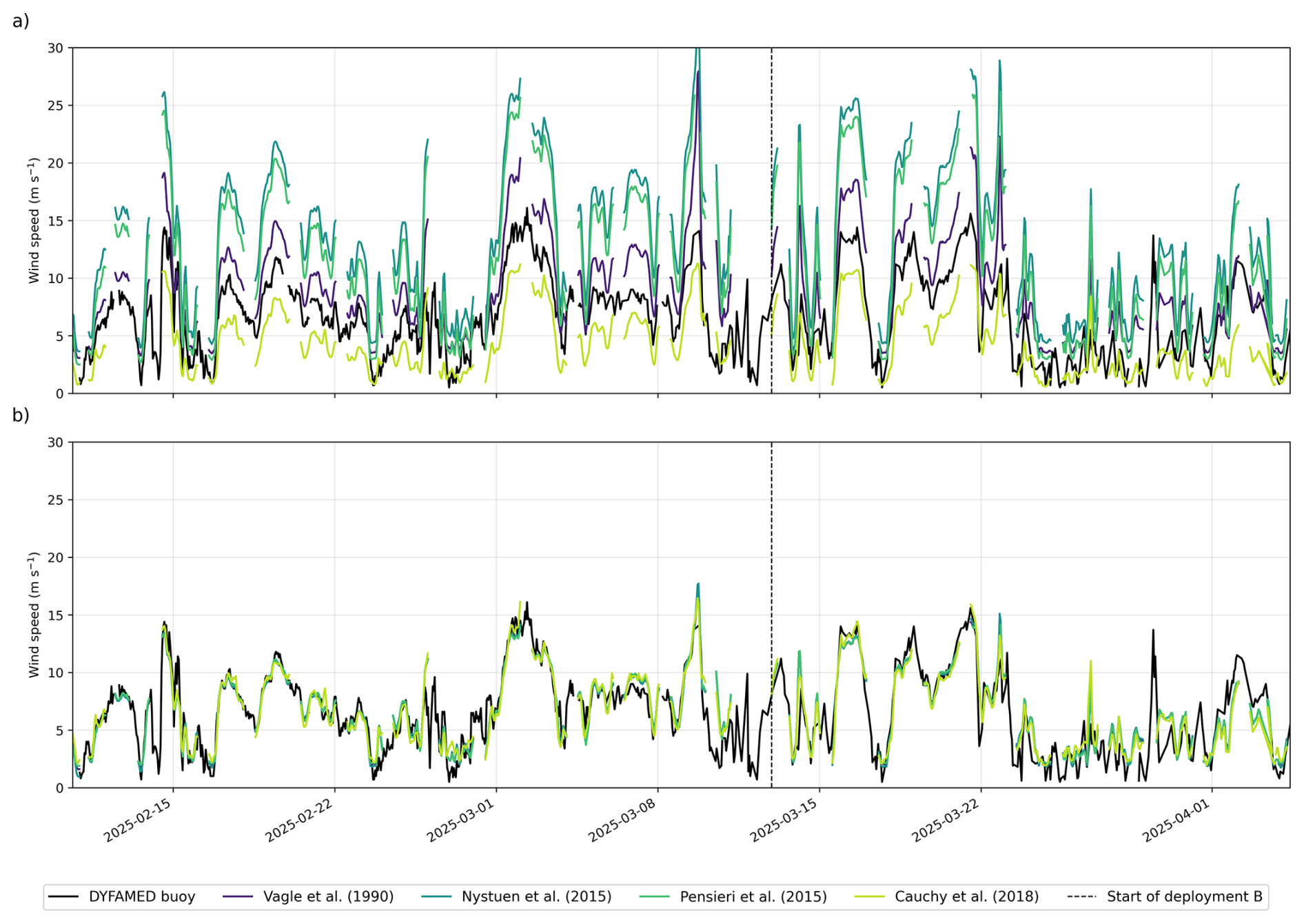
Figure 4 Comparison of unoptimized (top) and optimised (bottom) wind speed models against DYFAMED buoy observations. Each subplot shows modelled wind speed estimates from four literature models (Vagle et al., 1990; Nystuen et al., 2015; Pensieri et al., 2015; Cauchy et al., 2018) compared with collocated buoy wind data (black line). The unoptimized models (a) use original published coefficients, while the optimised models (b) are re-fitted using data within 40 km of the DYFAMED site. The dashed vertical line indicates the start of deployment B.

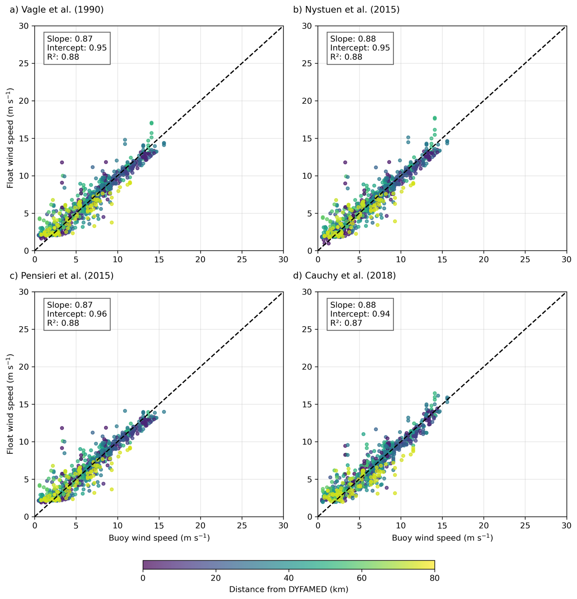
Figure 5 Comparison of optimised wind speed estimates from four literature models against collocated DYFAMED buoy wind measurements. Each subplot (a–d) shows scatter plots of float-derived wind speed vs. buoy wind speed using model-specific optimised coefficients: (a) Vagle et al. (1990), (b) Nystuen et al. (2015), (c) Pensieri et al. (2015), and (d) Cauchy et al. (2018). Points are color-coded by distance from the DYFAMED buoy, and the dashed line represents the 1:1 reference. Insets display linear regression slope, intercept, and coefficient of determination (R²).

However, even after successful fitting, the portability of acoustic–wind models remains uncertain. Factors such as noise contamination, ambient biological activity and regional propagation conditions can vary substantially between deployments, affecting both the shape and robustness of the acoustic–wind relationship (Gros-Martial et al., 2025b). Moreover, profiling floats introduce their own artifacts, which may arise from hydrodynamic turbulence, buoyancy engine activity, bubble release, or electronic interference, each of which can contaminate the acoustic signal independently of wind forcing. Even models developed in the same basin required refitting (i.e. Pensieri et al., 2015; Figs. 4, 5 and 7).

A promising direction would be to classify deployments into broader “acoustic environment types”, such as open-ocean gyres, coastal shelves, or high-latitude storm zones, within which shared model parameters could be defined and validated. This aligns with the priorities outlined in the Ocean Sound Essential Ocean Variable (EOV) Implementation Plan, which emphasizes the need for community-agreed metadata standards, calibration protocols, and classification schemes to support global comparability across acoustic deployments (Tyack et al., 2023). Evaluating these frameworks for profiling floats may help standardize acoustic wind retrieval and integrate it more effectively into global observing systems.

3.2 Generalizing float-specific wind modelling using reanalysis

While site-specific fitting of acoustic wind models yields accurate float-derived wind estimates, such fittings are not feasible in most regions of the global ocean where in-situ wind observations are unavailable. To assess whether the acoustic–wind relationship can be generalized for remote deployments, we investigated the use of reanalysis wind products as a proxy reference for model fitting. Specifically, we used the ERA5 atmospheric reanalysis (Bell et al., 2021) to refit the Nystuen et al. (2015) model to float-measured acoustic data, simulating a scenario where no collocated buoy or shipboard wind measurements are available (Figs. 6 and 8).

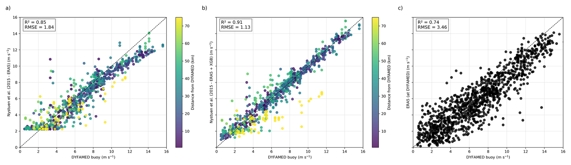
Figure 6 Comparison between DYFAMED buoy wind speed measurements and float-derived estimates using the Nystuen et al. (2015) acoustic model: (a) wind speeds estimated using Nystuen's polynomial formulation fit to ERA5; (b) same model corrected using a residual-learning approach with XGBoost, trained on the differences between ERA5-based estimates and DYFAMED observations; and (c) ERA5 wind speed at the DYFAMED grid point compared directly to buoy measurements for February, March and April 2025. Each point is colored by the float's distance from DYFAMED in panels (a) and (b). Dashed lines denote 1:1 agreement. All wind speeds are expressed in meters per second (m s⁻¹).

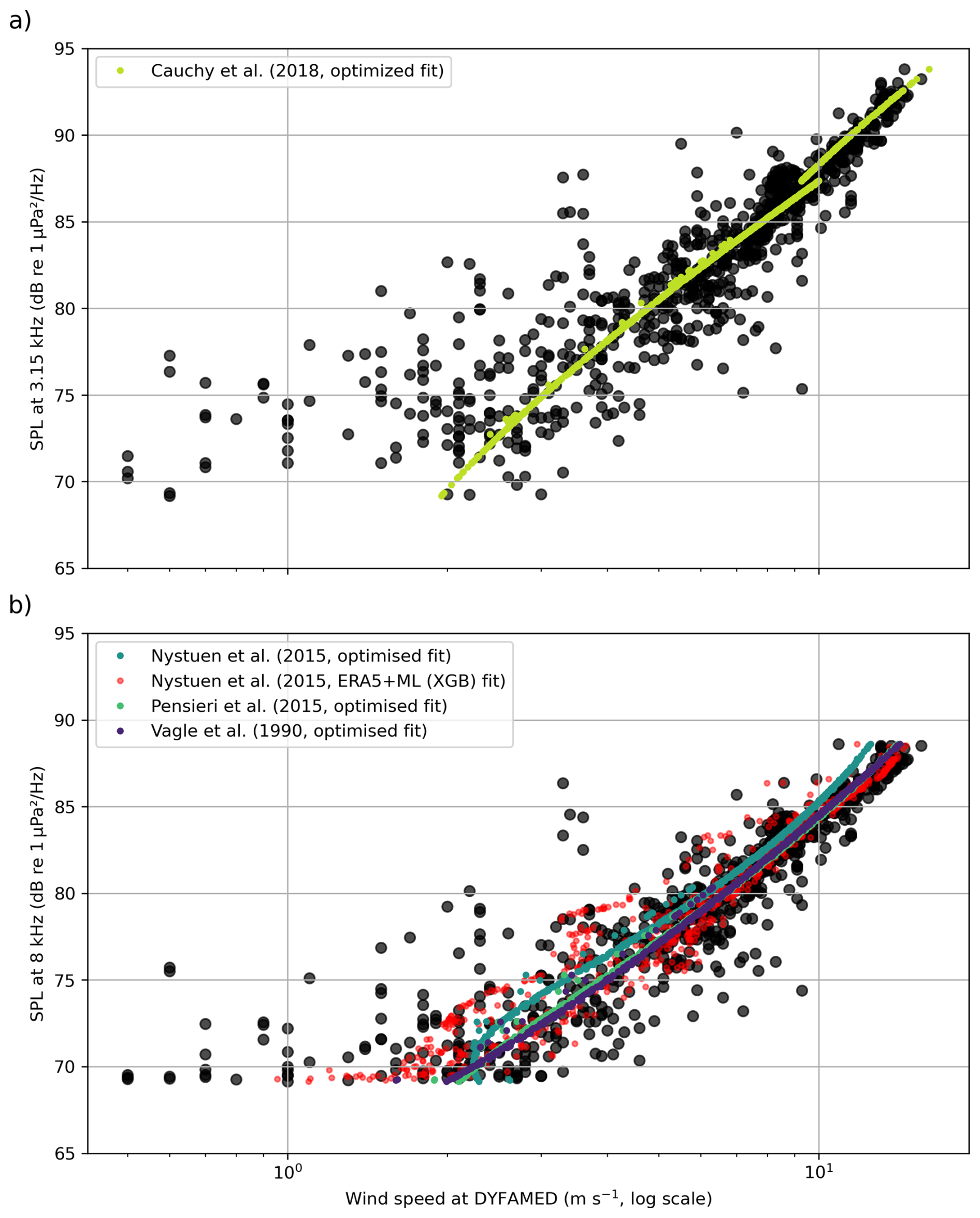
Figure 7 Optimised 10 m wind speed (log scale) as a function of observed underwater sound pressure level (SPL) at DYFAMED for (a) 3.15 kHz and (b) 8 kHz. Observed wind speed is shown in black.

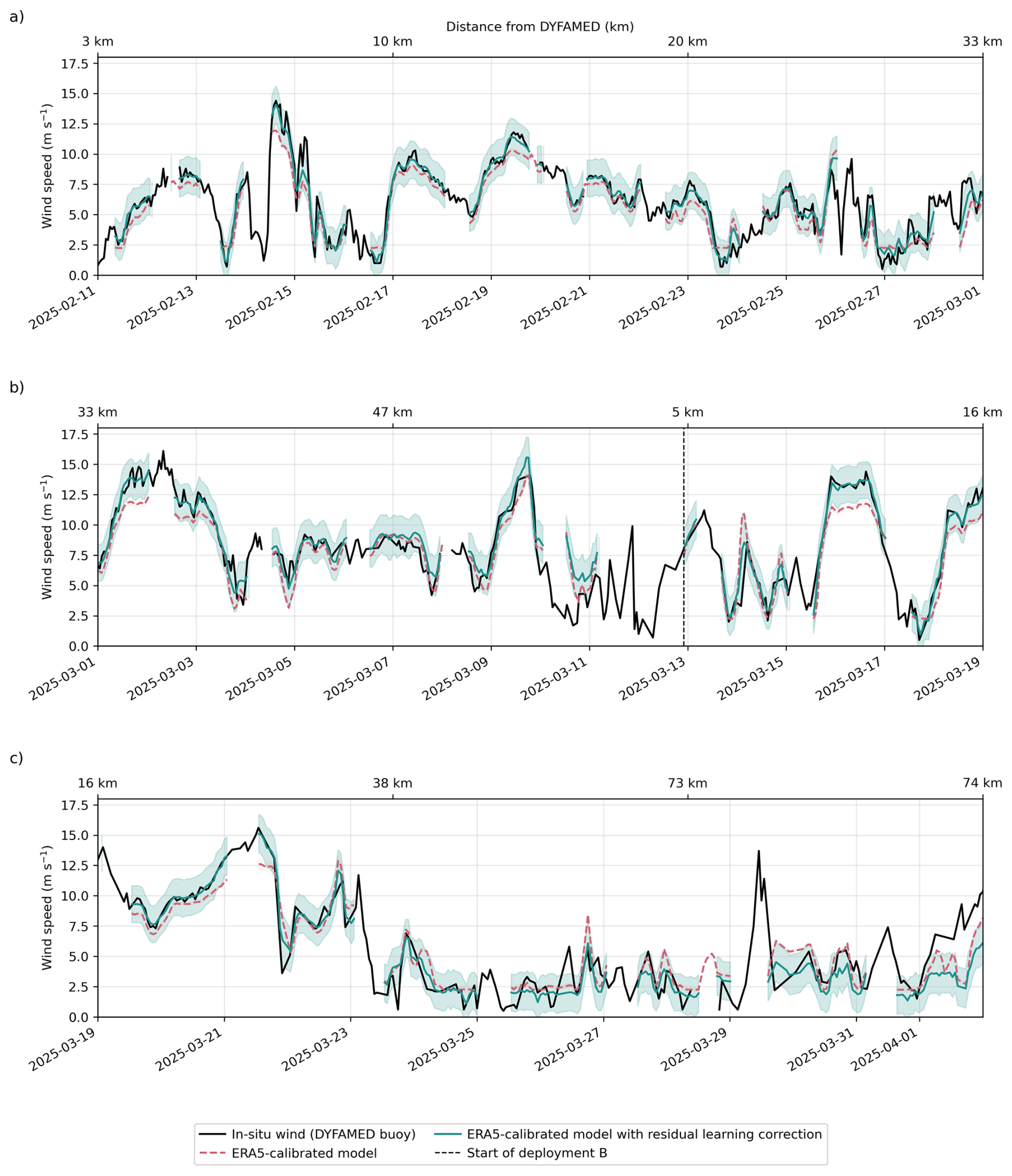
Figure 8 Time series comparison between acoustic float wind estimates and DYFAMED buoy winds, displayed over three consecutive 18 d windows (a–c). The dashed pink curve corresponds to wind speeds predicted using the Nystuen et al. (2015) acoustic model calibrated solely with ERA5 reanalysis winds. The solid blue line shows the same model after applying the residual-learning correction (XGBoost), and the shaded region indicates its associated predictive uncertainty. Buoy-measured wind speed is shown in black. The upper x-axis reports the float's distance from DYFAMED throughout the record, and the dashed vertical line indicates the transition to deployment B.

Using time-matched float sound pressure level at 8 kHz and collocated ERA5 wind speed, we derived a new set of coefficients (Sect. 2.6), producing a general-purpose fit based solely on float data and reanalysis inputs. The goal was to test whether an existing model can be adapted for use in data-sparse regions, enabling scalable wind estimation from profiling floats.

As shown in Fig. 6a, the ERA5-calibrated Nystuen et al. (2015) model reproduced wind variability within the 2.5–10 m s⁻¹ range with moderate skill (R²=0.85), and performed best during Deployment A, when wind conditions remained relatively stable (Fig. 8). Performance deteriorated during stronger wind events, particularly in Deployment B, where the model systematically underestimated wind, with errors > 3 m s⁻¹ (Figs. 6a and 8).

Comparison with DYFAMED also revealed broader limitations of ERA5. Although ERA5 provides a globally consistent wind product, it diverged from buoy observations during several high-wind episodes (Figs. 6c, 8). This behaviour is consistent with earlier reports of reanalysis underestimating localised, orographically forced winds in semi-enclosed basins such as the Mediterranean (Bentamy et al., 2003; Bell et al., 2021). Such biases are critical in regions like the Southern Ocean, where frequent high-wind events dominate air–sea CO₂ fluxes and gas exchange scales nonlinearly with wind speed (Wanninkhof, 2014; Wanninkhof et al., 2025).

Thus, while float reanalysis-based calibration enables acoustic wind estimation in the absence of local observations, its accuracy depends strongly on the reliability of the reference product used for fitting.

3.3 Simulating scalable wind estimation in data-sparse regions

While reanalysis-calibrated acoustic models offer a pathway for estimating surface wind speed in remote regions, the results in Sect. 3.2 show that this approach alone is insufficient during high-wind or rapidly evolving events. This limitation is especially critical in high-latitude regions such as the Southern Ocean, where extreme wind forcing drives critical fluxes of heat, momentum, and carbon (Gray et al., 2018; Dotto et al., 2019; Zhang et al., 2022; Gruber et al., 2023).

3.3.1 Local model correction using residuals learning

To overcome this, we implemented a residual learning framework that combines the generalizability of reanalysis-based fitting with the accuracy of localized corrections. Specifically, we trained an ensemble of XGBoost regression models to predict the residuals between the ERA5-calibrated estimates and collocated DYFAMED buoy observations (see Sect. 2.6). The model was trained using float data within 40 km of DYFAMED and bootstrapped over 100 iterations to quantify mean corrections and prediction uncertainty (Figs. 1, 6b). The 40 km radius was selected based on the sensitivity analysis of Cauchy et al. (2018), who found it to balance proximity with data availability; though this threshold is likely site-dependent and should be reassessed in future deployments.

The corrected wind time series showed substantially better agreement with DYFAMED observations (Fig. 8), especially during high-wind events where the uncorrected model underestimated wind speeds. This bias correction increased R² from 0.85 to 0.91 and reduced RMSE from 1.84 to 1.13 m s⁻¹, a 38.6 % reduction in prediction error. While other learning-based methods have achieved similar improvements (e.g., Zambra et al., 2023, 16 % RMSE reduction), our method explicitly uses reanalysis as a prior and relies only on sparse in-situ fitting, making it more realistic for remote deployments.

The machine learning model does not estimate wind speed directly but instead learns to adjust biases using a small set of predictors (i.e. acoustic signal intensity, deployment day, ERA5-calibrated prediction). In effect, it identifies conditions under which ERA5 is likely to fail, applying larger corrections during high-wind events.

These results demonstrate that even limited in-situ reference data – for example, brief engine-off ship-based winds during deployment – can significantly improve estimates along the full float trajectory. In our case, in-situ points represented approximately 40 % of the record due to the short deployment but this introduces potential limitations. First, because fitting and evaluation used the same dataset, the performance metrics may be optimistic. Future deployments should use spatially or temporally separate validation or fully independent reference stations. Second, the RMSE reduction reflects improvements mainly at high wind speeds, where raw errors are largest, and may overstate gains at lower winds. Taken together, these factors imply that these performance metrics likely represent an upper bound of the framework's accuracy for long-duration or multi-region deployments. The generalisation across sites, seasons and events remains untested and will require validation using spatially or temporally independent datasets.

3.3.2 Strategies for sparse in-situ calibration

In practical terms, acquiring suitable reference observations can be challenging. While ship-based wind measurements are a natural candidate, particularly during float deployment or recovery, they may be unsuitable for model fitting if the ship is too close, as engine noise can contaminate the float's acoustic signal. A practical compromise is to station the ship far enough to avoid acoustic interference while keeping wind measurements representative. Alternatively, a more robust strategy is to deploy floats in proximity to existing meteorological buoys, which provide collocated wind observations without interfering with subsurface acoustic recordings.

In regions where neither buoys nor suitable ship data are available, identifying whether the available in-situ coverage is sufficient becomes more complex. This will depend not only on the duration and trajectory of the float mission, but also on the opportunistic use of additional reference sources encountered along the way, for example, other buoys, or wind observations from vessels transiting the area. Where such sources are absent, satellite products, particularly synthetic aperture radar (SAR), can provide episodic but high-resolution wind fields that capture localized variability and serve as intermittent calibration points.

More broadly, these scenarios highlight the need for flexible modelling approaches that can exploit heterogeneous and temporally limited reference data. Rather than relying on dense training datasets or persistent surface observations, future efforts could employ machine-learning strategies such as domain adaptation, transfer learning, or few-shot learning to adapt models to new environments with minimal retraining. For instance, recent work by Wang et al. (2020) has shown that few-shot transfer methods can yield competitive performance even when only a small number of target-domain samples are available.

In the context of profiling floats, such strategies could enable a more scalable approach to acoustic model tuning, leveraging sparse data from ships, buoys, or satellites, each limited individually but collectively offering adequate diversity. We propose framing this as opportunistic multisource model fine-tuning: a hybrid calibration scheme in which local corrections are derived from whatever reference sources are available, without requiring dense or continuous in-situ coverage. Developing and validating such approaches will be essential for global deployment of acoustically equipped floats while maintaining robustness across diverse environmental and acoustic conditions.

3.3.3 Implications for global observing

While ERA5 provides a useful climatological reference, it tends to underestimate short-lived, high-wind events due to spatial and temporal smoothing (Fig. 8). This is an issue particularly for gas exchange studies, as extreme winds disproportionately contribute to total fluxes. Acoustic float data, collected continuously and at high resolution, offer the potential to complement satellite or reanalysis wind products, particularly during short-lived wind events that are smoothed out in coarse-resolution products.

However, model performance degrades with increasing distance from DYFAMED, reflecting the spatial decorrelation of wind fields and the limited spatial representativeness of the buoy observations. Beyond 73 km during Deployment B, both the Nystuen et al. (2015) – ERA5 fit and the machine-learning-corrected float estimates begin to diverge from DYFAMED winds (Figs. 6 and 8). This divergence likely reflects true spatial variability rather than model failure, as the float and buoy may be sampling different wind regimes. One way to address this uncertainty is to analyse float trajectories that pass between two surface reference stations, testing whether refitting at the final station yields consistent corrections or reveals systematic regional shifts in wind decorrelation. Such an approach will require future deployments that span multiple buoys, enabling a systematic evaluation of how model performance degrades, or remains robust, across both time and space.

Additionally, in the Southern Ocean, where anthropogenic noise is relatively low, lower-frequency bands (< 1 kHz) may be viable for wind estimation, as they are more sensitive to high wind speeds due to increased bubble activity and longer propagation ranges. These bands could outperform higher-frequency bands under strong forcing conditions, provided contamination from distant shipping or other sources remains minimal.

Several recent studies have applied machine learning to underwater acoustic data to estimate wind and rainfall, often relying on long-term, stationary deployments and direct spectral prediction (Taylor et al., 2020; Trucco et al., 2022; Trucco et al., 2023; Zambra et al., 2023). While effective under controlled conditions, these approaches depend on dense labelled datasets and assume stable acoustic environments. In contrast, our residual-learning strategy is designed for sparse, mobile deployments: it corrects reanalysis-based estimates using short-duration in-situ fitting and does not require full acoustic labels, making it more compatible with the operational realities of profiling floats.

While in-situ data remains the most difficult to obtain in remote regions, our method supports opportunistic fitting, for example, brief ship-based winds during deployment or nearby meteorological buoys. This hybrid strategy balances scalability and realism, enabling more robust performance even where long-term reference data are scarce.

Another important consideration is the potential for regional bias introduced by the depth correction applied to acoustic levels. This correction compensates for effects driven by local hydrographic structure and was derived from the float's mean profile at the start of the deployment. Applying a single correction to the full mission introduces a location-dependent bias that may vary across floats or seasons. Ideally, the correction should be recalculated with each new hydrographic profile, especially for long-term or wide-ranging deployments. To ensure basin- to global-scale comparability, these corrections should be standardised and explicitly documented in processing protocols for acoustic-equipped floats.

This deployment-focused flexibility is key to scaling up acoustic wind estimation globally. By combining reanalysis for first-order fitting with localized corrections when available, our framework improves agreement with in-situ winds without requiring long-term surface infrastructure. Scaling this approach across the BGC-Argo array would provide high-resolution, all-weather wind monitoring in regions poorly served by existing observing networks.

4 Conclusions

This study provides a proof of concept for retrieving surface wind speeds from subsurface ambient noise recorded by a profiling float equipped with a passive acoustic sensor and operated alongside standard biogeochemical sensors. Float-measured acoustic noise captured surface wind variability from 500–1000 m depth, and empirically calibrated estimates closely matched buoy observations, confirming the feasibility of subsurface acoustic wind retrieval. Reanalysis-based calibration reproduced moderate winds but underestimated high-wind events, highlighting the limits of using reanalysis alone in dynamic environments. A residual-learning correction using sparse local reference data substantially improved performance, particularly during strong winds. These findings underscore the potential of acoustic-equipped profiling floats to provide scalable, high-resolution wind observations in remote regions, supporting improved estimates of wind-driven air–sea fluxes.

Nevertheless, our results stem from a single short-duration deployment. Broader validation across regions, seasons, and acoustic environments is needed, and performance estimates likely represent an upper bound. Recent benchmarking efforts (e.g., Gros-Martial et al., 2025b) already demonstrate the value of assembling multi-site acoustic–meteorological datasets and highlight the challenges of model transferability across diverse soundscapes. Future missions should employ independent training–validation–test partitions to rigorously evaluate generalizability, following best practices established in recent WOTAN studies that explicitly address temporal correlation and multi-site validation requirements (e.g., Cauchy et al., 2018; Taylor et al., 2020; Trucco et al., 2022; Trucco et al., 2023).

Acoustic wind retrieval offers a promising pathway for expanding autonomous wind monitoring within the global BGC-Argo array, improving coverage in regions poorly served by existing systems. Sparse in-situ calibration also provides a valuable new data stream for validating and potentially correcting regional biases in global wind reanalyses. Ultimately, this work supports the Ocean Sound EOV's call for standardized methodologies and demonstrates the feasibility of integrating passive acoustics into sustained, basin- to global-scale observing systems.