Atlantic Water flow through Fram Strait to the Arctic Ocean measured by repeated glider transects

We present transport estimates of Atlantic Water (AW) and Recirculating Atlantic Water (RAW) across a zonal transect at 77°15^′ N using repeated ocean glider observations. Over three missions during autumn and winter of 2020 to 2022, 22 high-resolution sections were collected, enabling detailed characterization of circulation branches and volume transport. On average, the West Spitsbergen Current (WSC) and the Front Current each transport approximately 2.5 Sv of AW (Θ>2 °C, $S_{\mathrm{A}}>\mathrm{35.06}\mathrm{g}{\mathrm{kg}}^{-\mathrm{1}}$) northward, yielding a combined net flux of about 5 Sv toward the Arctic. Variability in transport and current structure is substantial and appears linked to atmospheric forcing. Case studies reveal that anomalous northward wind stress coincides with peak AW transport, roughly twice the seasonal mean, consistent with Ekman dynamics and elevated sea surface height along the coast. Conversely, strong southward wind stress weakens the WSC and nearly eliminates the Front Current. Transport of RAW (Θ>0 °C, $S_{\mathrm{A}}>\mathrm{35.06}\mathrm{g}{\mathrm{kg}}^{-\mathrm{1}}$) west of the Front Current is estimated to be about 1 Sv, but this does not capture the expected stronger recirculation transport further west, beyond the glider's target transect. These results highlight the capability of gliders to resolve spatial variability in boundary currents that mooring arrays cannot capture. Extended seasonal coverage, including summer, is needed to assess transport variability under peak wind forcing.

1 Introduction

Poleward flow of Atlantic Water (AW) from the Nordic Seas is the main contributor of oceanic heat and salt into the Arctic Ocean (Aagaard et al., 1987; Rudels, 2015), with far reaching effects on sea ice cover, ocean stratification and ecological environments (Ingvaldsen et al., 2021; Polyakov et al., 2025). Fram Strait, located between Greenland and Svalbard, is the deepest connection between the Arctic Ocean and the Nordic Seas, and the main pathway for AW into the Arctic.

The circulation patterns of AW in Fram Strait are complex (Fig. 1). To monitor the ocean currents, and temperature and salinity structure in this passage, an array of oceanographic moorings has been maintained at 78°50^′–79° N since 1997 as a joint effort between the Alfred Wegener Institute and the Norwegian Polar Institute (Schauer et al., 2004; Beszczynska-Möller et al., 2012). The measurements from this array have been used to quantify the volume and heat fluxes, and their variability at this section. These moorings have provided observations with high temporal resolution over long time periods, and given insight into long-term changes as well as seasonal and short-term variability in circulation and hydrography in Fram Strait (Beszczynska-Möller et al., 2012; von Appen et al., 2016). The lateral and vertical resolution of instrumentation in the mooring array is, however, relatively coarse and does not capture the detailed horizontal structure of currents and hydrography. Here, we analyze observations from repeated ocean glider sections taken during three consecutive years (Fer et al., 2025) with the aim to resolve the lateral and vertical structure of the AW flow and its variability in Fram Strait. These observations have a horizontal length scale of order 1 km and vertical scales of 1 m, which complements the high temporal resolution provided by the mooring array.

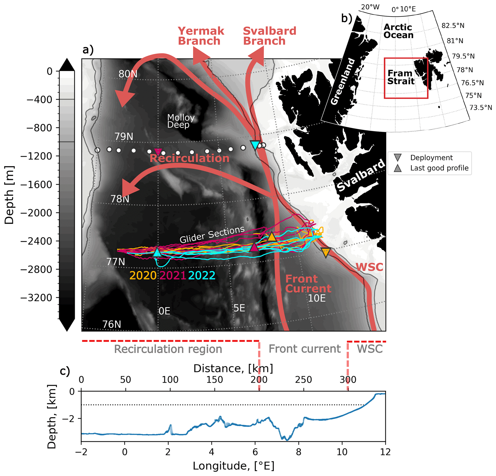
Figure 1 (a) Bathymetry in Fram Strait (Jakobsson et al., 2020) including sections from glider mission 1 (2020, yellow), mission 2 (2021, pink), and mission 3 (2022, cyan). Locations of deployment (∇) and the last good profile (Δ) are indicated in corresponding colors. Circulation pattern of the warm Atlantic current including the West Spitsbergen Current (WSC), the Front Current, the Yermak Branch, the Svalbard Branch and Recirculation branches are indicated based on our observations and observations from the literature. The −400 and −1000 m isobaths are highlighted. White circles indicate the location of moorings in the 78°50^′ array (Beszczynska-Möller et al., 2012). (b) Location map showing the study the region and the boundaries of panel (a) in red. (c) The bathymetry along the target section. The dotted black line indicates the glider's maximum depth of 1000 m. Selected boundaries at 200 and 300 km distance along the transect (dashed red lines) delineate the different current regions.

AW is brought into Fram Strait by the Norwegian Atlantic Current system comprised of the Norwegian Atlantic Slope Current flowing along the shelf break of Norway and the Barents Sea opening, and the Norwegian Atlantic Front Current following the Mohns and Knipovich ridges (Orvik and Niiler, 2002). Both branches are guided by topography, but the front current is a surface-intensified baroclinic jet, while the slope current is more barotropic. Along the southern West Spitsbergen Shelf edge, the slope current is referred to as the West Spitsbergen Current (WSC). Along the west coast of Svalbard, parts of the AW carried by the WSC can diverge from its core, intruding eastward onto the West Spitsbergen Shelf and further toward the adjacent fjords (Frank et al., 2025), effecting the regional hydrography, marine biosphere, sea ice variability as well as melting and calving rates of marine-terminating glaciers. As the offshore topographic contours converge near 78° N, the Front Current branch merges into the WSC (Orvik and Niiler, 2002; Walczowski et al., 2005). Approximately half of the AW in Fram Strait enters the Arctic Ocean whereas the remaining AW recirculates and joins the southward flowing East Greenland Current (Quadfasel et al., 1987; Manley, 1995; Dale et al., 2024). As a consequence of the recirculation, warm temperature anomalies in the WSC partly control Atlantic Water temperatures on the Northeast Greenland continental shelf, which in turn control the melt rate of major glaciers in the region (McPherson et al., 2023).

Based on the mooring observations, the average structure of the currents carrying AW at 79° N can be described by three components: (i) The WSC core (or the Svalbard branch), which is an extension of the slope current and flows on the upper shelf slope, (ii) an outer offshore branch which is an extension of the front current and extends to the shelf rise, and (iii) several recirculating branches mid-strait (Fig. 1a, Beszczynska-Möller et al., 2012). The outer branch is referred to as the Yermak branch north of 79° N. Recirculation of AW captured by moorings along the prime meridian is relatively continuous at 78°50^′ N, but is characterized by passing eddies at 80°10^′ N (Hofmann et al., 2021). Eddy-resolving numerical models show that the bulk of the recirculation occurs along two pathways between 78 and 81° N (Hattermann et al., 2016; Wekerle et al., 2017): one along the Spitsbergen Fracture Zone and south of the Molloy Hole and the other is located along the Molloy Fracture Zone and north of the Molloy Hole (Fig. 1a).

At the Fram Strait mooring array, the average (1997–2010) northward volume transport of water warmer than 2 °C is 3.0±0.2 Sv (Sverdrup, 1 Sv ≡10⁶ m³ s⁻¹), showing a strong seasonal signal with summer averages approximately doubling in late autumn and winter due to variability within their defined offshore WSC branch (Beszczynska-Möller et al., 2012). Out of these 3 Sv, 1.3±0.1 Sv is carried in the WSC core (Beszczynska-Möller et al., 2012), and the remaining can be considered to contribute to the recirculation and the Yermak Branch. Consistently, further north, at roughly 80° N after the circulation branches separate (Fig. 1a), year-round observations from moorings on the southern slope of the Yermak Plateau show an average AW transport of 1.1±0.2 Sv with a maximum in autumn (1.4±0.2 Sv), and a minimum in summer (0.8±0.1 Sv, Fer et al., 2023).

Moorings provide highly valuable time series of oceanic conditions, but their limited lateral and vertical resolution introduces substantial uncertainty in AW transport estimates. For instance, moorings may fail to capture the current core, leading to underestimation of AW fluxes, while coarse estimates of current width can result in both over- and underestimations. It is also difficult to determine whether observed fluctuations in current strength and hydrographic properties reflect lateral shifts in the core's position or actual changes in its properties. Ship-based hydrographic and current sections help address these questions, but such data are generally collected during summer, and therefore not a good representation of annual variability. Repeated observations with high lateral and vertical resolution are essential, yet traditionally lacking. Ocean gliders help fill this gap by providing data with the required spatial coverage and resolution.

Ocean gliders (gliders hereafter) have become widely-used platforms enabling ocean research and sustained observation at relatively fine horizontal scales (Rudnick, 2016). A glider is a buoyancy-driven, remotely-piloted autonomous vehicle, which profiles in a sawtooth trajectory as it travels between way points (Eriksen et al., 2001; Rudnick, 2016; Testor et al., 2019). A glider changes its buoyancy to profile vertically, typically to 1000 m depth and slanted at 20 to 30°. Wings generate hydrodynamic lift force with a horizontal component propelling the glider horizontally. A glider covers 𝒪(100) km transects (e.g. covering a boundary current) in about 4 d, providing profiles with horizontal separation of 1 to 4 km and vertical resolution of 1 to 5 m.

Here, we use fine-resolution spatial data collected using gliders that were operated in Fram Strait from autumn to winter for three years between 2020 and 2023, repeating sections along 77°15^′ N. We present average current and hydrography fields, and the AW volume transport in the WSC, the Front Current and the Recirculation region throughout the glider missions, and discuss their variability in relation to atmospheric forcing.

2 Data and methods

2.1 Glider data

We analyze data from three glider missions in Fram Strait, conducted between October 2020 and February 2023, using 1000 m rated Seagliders, operated by the Norwegian Facility for Ocean Gliders at the Geophysical Institute, University of Bergen. Seaglider is a widely-used type of ocean glider (Eriksen et al., 2001). The glider data together with a detailed description of data processing, calibration and quality control are available from Fer et al. (2025).

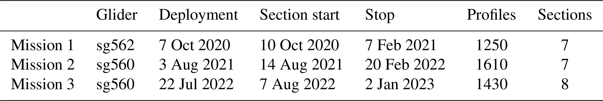
The target section was selected to capture the front and slope branches before they merge, enabling separate estimates of their volume transport and variability. It was located at 77°15^′ N between 2° W to 12° E. Deployments were made from a ship of opportunity at locations close to the target section that were also convenient for the ship's cruise plan. As a result, there is a period during which the glider was in transit toward the target section at the beginning, or toward the recovery location at the end of each mission. In 3 missions, a total of 22 sections were collected. Of these, five sections are incomplete, mainly because of recovery and deployment transits. Mission details are summarized in Table 1.

During the first mission (7 October 2020–8 February 2021), the glider completed 625 dives and collected 1250 profiles before entering recovery mode. The second mission (3 August 2021–10 March 2022) included 805 dives (1610 profiles), with science operations ending on 20 February. The third mission (22 July 2022–8 February 2023) performed 960 dives (1920 profiles), but science data collection stopped after dive 715 (profile 1430) on 2 January to conserve battery for recovery. We only use the profiles from the target section in our analysis and exclude the periods when the gliders were in transit. The transit period to the target section was longest, approximately two weeks, during mission 3. Missions were conducted primarily during autumn and winter, and are separated by a gap of five to six months.

The gliders operated between the surface and 1000 m depth, or 10 to 15 m above seafloor for shallower depths, sampling during both dives and climbs. The vertical velocity was typically 10 cm s⁻¹. The gliders were equipped with a Kistler pressure sensor, a Sea-Bird Scientific CT Sail (unpumped) measuring conductivity and temperature, and an Aanderaa dissolved oxygen sensor. The sampling rate of the sensors was variable. Typically the CT sail sampled every 10 s in the upper 300 m, 15 s between 300 and 600 m, and 20 s between 600 and 1000 m. The optode sampled a factor of five slower, every 50, 75 and 100 s, respectively. The vertical resolution of the temperature and conductivity profiles are ∼1 m in the upper 300 and ∼1.5 m from 300 to 600 m. The data set was processed using the Seaglider Basestation3 (v3.0.4) software, including a hydrodynamic flight model regression, correction for the thermal lag of the conductivity cell, and quality control. Temperature and salinity profiles, as well as the derived density, are quality controlled, first using automated routines, and then applying additional despiking and manual quality control, as detailed in the data files.

In our data set, the mean (± one standard deviation) horizontal spacing at the surface of subsequent downward (dive) and upward (climb) profiles was 3.5±2.3 km and 5.3±2.0 h. The spacing of the profiles is primarily set by the profiling depth, which ranged from approximately 150 to 1000 m (99 % of all profiles were deeper than 150 m). The average duration for a glider to sample the target section is 23 d (based on the 15 sections with >80 % coverage of the target section). Sampling the WSC and the Front Current region takes on average 9 d (based on 21 sections with >80 % coverage). The main reason that not all sections cover the full target section is because of the opportunistic deployment and recovery location of the gliders.

Table 1 Deployment details for the three missions. “Section start” is the start date of the first profile on the target section and the “stop” date is the date of the last good profile in a mission. Additional information can be found in the metadata of the data files in Fer et al. (2025).

After initial processing, the profile data were averaged onto the target section using bins of 2 km in width and 2 dbar in pressure (approximately 2 m depth). The section spans 342 km in longitude. We define the horizontal eastward distance along the target section starting from 2° W and refer to it as “distance” hereafter. Gridding is based on distance. East of 300 km (∼10° E, ∼1600 m isobath), however, currents are strongly influenced by the steep bathymetry near the continental shelf break. Profiles collected in this region are assigned to their corresponding isobaths and distance on the target section before gridding. This is a typical method when gliders are advected by boundary currents that are guided by topography. Profiles sampled more than 30 km away from the target section are discarded.

We construct horizontal distance versus depth sections of measured variables using an objective interpolation algorithm using the GliderTools package for Python (Gregor et al., 2019). We estimate horizontal (40 km) and vertical (40 m) length scales, the nuggets (temperature: 0.1075, salinity: 0.0012) and partial sills (temperature: 0.3105, salinity: 0.0025) using GliderTools' semivariance function over a region that captures northward Atlantic Water variability (20 to 200 m depth and 230 to 340 km distance). These parameters are then applied for objective mapping of the gridded data fields to the target section. We thus have 22 mapped sections of the target transect.

In season-specific calculations, autumn and winter are defined as the parts of a mission before or after 15 November. To keep a section intact, if it includes 15 November, the section is assigned to the season it contains the most observations from. One section exclusively contains data from August and is thus disregarded from season-specific estimates.

Absolute Salinity S_A, Conservative Temperature Θ, and potential density anomaly σ₀ are obtained using TEOS-10 and the Gibbs Seawater toolbox for Python (McDougall and Barker, 2011). Velocity-weighted temperature and salinity are defined as:

$$\begin{array}{}\text{(1)}& Y={\displaystyle \frac{\sum v_{\mathrm{g}}(x,z)y(x,z)\mathrm{\Delta }x\mathrm{\Delta }z}{\sum y(x,z)\mathrm{\Delta }x\mathrm{\Delta }z}},\end{array}$$

where Y is the velocity-weighted temperature or salinity, v_g(x,z) is the velocity field, y(x,z) is the temperature or salinity field, and Δx and Δz are the horizontal and vertical resolution of the gridded data.

2.2 Geostrophic currents

Geostrophic shear of the horizontal velocity component perpendicular to the target section is calculated from the thermal wind equation, using the horizontal slope of density surfaces from the final gridded and objectively interpolated glider data with the Gibbs Seawater (GSW) Oceanographic Toolbox (McDougall and Barker, 2011). The smoothing length scales applied to the hydrographic data are appropriate for geostrophic calculations.

To obtain absolute geostrophic currents, accurate reference currents representative of barotropic flow are required. Typically, glider-based depth-averaged currents (DAC) over the upper 1000 m, smoothed over the same horizontal scale as the hydrographic data, can be used. However, during the first half of the second mission, DAC estimates exhibit erroneous values: northward currents are anomalously strong across the full transect for several months (Fig. A1b), a pattern not confirmed by independent ocean monitoring and forecasting fields from the Copernicus Marine Service or by mooring data at 79° N (Rebecca McPherson, personal communication, 14 November 2024).

Outside this period, depth-averaged currents from the glider agree well with surface geostrophic currents from the gridded altimeter product (Global Ocean Gridded L4 Sea Surface Heights And Derived Variables Reprocessed 1993 Ongoing, 2024, horizontal resolution 0.125°) calculated from the slope of the absolute dynamic height using a geostrophic balance (Fig. A1). Therefore, for consistency, we combine baroclinic currents estimated from glider hydrography data with the surface geostrophic currents from the altimeter product for all sections to obtain absolute geostrophic currents.

Mork and Skagseth (2010) used repeated hydrographic data in the Svinøy section (at 62° N off the coast of Norway) with absolute dynamic sea surface topography data to quantify the mean flow and the variability in the slope and front branches of the Norwegian Atlantic Current. For the slope branch, the estimated currents agreed well with the current measurements within the error range, but they were approximately 15 % lower and the lateral structure was smoother, as a result of the relatively coarse resolution and the gridding of the altimeter data. Excluding the first half of Mission 2 (sections 7 through 10) with erroneous DAC estimates, the absolute depth-averaged current estimated by the gliders is, on average, 4 % weaker than the satellite altimetry estimates. The difference between the volume transports estimated using DAC from the glider and the surface current from the altimetry is generally less than one standard deviation of the two estimates (not shown), lending credibility for using the satellite derived values for the full data set.

2.3 Atmospheric forcing

We use hourly output of wind stress and sea ice concentration from ERA5 reanalysis (Hersbach et al., 2023). Wind stress curl is estimated from the wind stress vector and the uniform 0.25°×0.25° horizontal resolution, using $\mathrm{\nabla }\times \mathit{\tau }=\mathrm{\Delta }{\mathit{\tau }}_y/\mathrm{\Delta }x-\mathrm{\Delta }{\mathit{\tau }}_x/\mathrm{\Delta }y$. When presenting zonal sections of wind stress and wind stress curl we average meridionally between 76°30^′ N and 78° N and temporally over the time a glider traveled between the eastern boundary and 200 km, which is the western boundary of the Front Current in our study. When presenting the full horizontal wind stress field, the same temporal averaging is used. Wind stress timeseries extracted in our study region, covering the period of the three glider missions are shown in Fig. 2, and present context for the wind forcing conditions over three years. The variability in AW volume transport in relation to wind stress forcing is discussed in Sect. 3.4.

During the mission years (2020–2022), the average wind stress across the target transect was directed southwestward, with a magnitude of 0.08 N m⁻² (Fig. 2). A pronounced seasonal cycle is evident from 2020 through 2022, with strong southward wind stress reaching nearly 0.3 N m⁻² in spring. Only the onset of these strong wind periods are captured at the end of glider missions two and three (Fig. 2a). The average conditions during the mission years are representative of the long-term average (Fig. A4). Average wind stress obtained from ERA5 between 1979 and 2024 is $-\mathrm{0.04}\pm \mathrm{0.07}\mathrm{N}{\mathrm{m}}^{-\mathrm{2}}$.

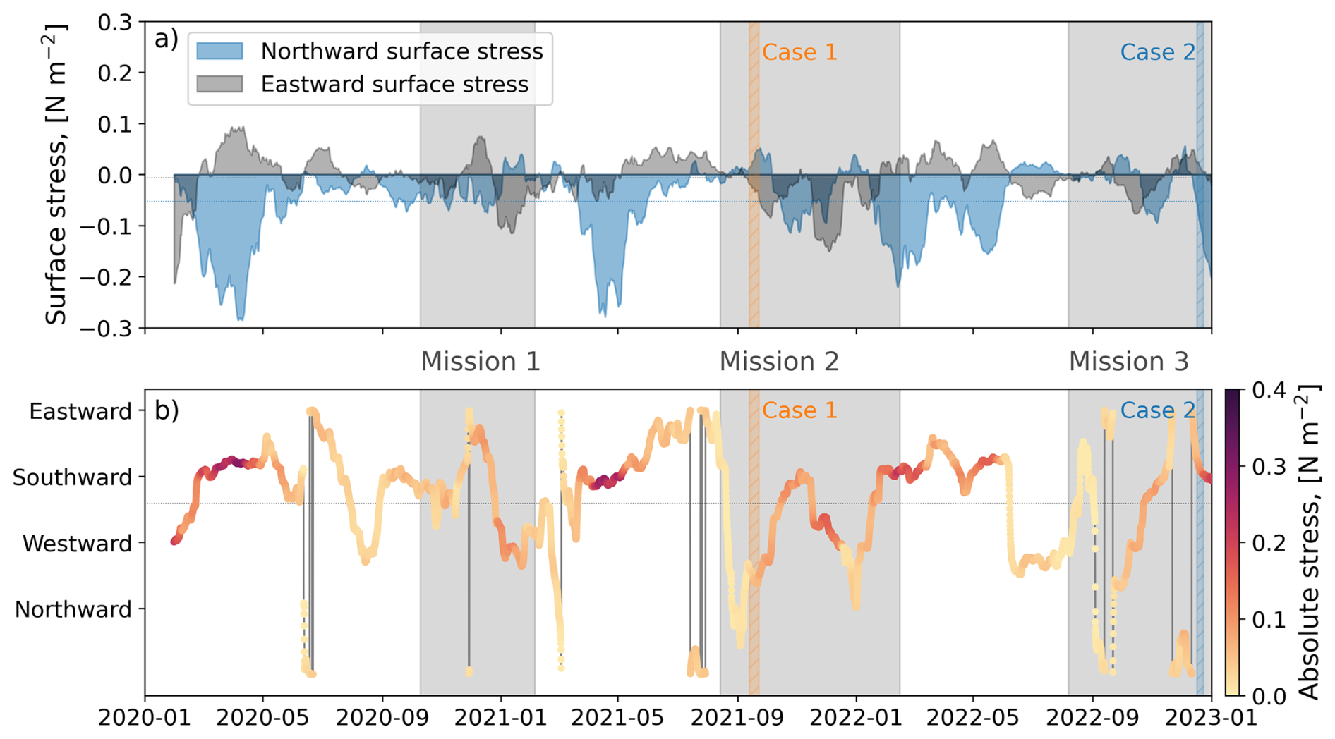
Figure 2 30 d rolling averages of surface stress (Hersbach et al., 2023) averaged over 2°  W–12° E and 77.25° N±0.25° N. (a) Northward (blue) and eastward (grey) average surface stress, and (b) its direction (grey line) and absolute magnitude (color). In both panels, the mission periods are indicated with grey background and the two case study periods are indicated by orange and blue hatched bars. The thin dotted horizontal lines in (a) indicate the mean northward (blue) and eastward (grey) stress, and (b) the mean stress direction (grey).

2.4 Identification of circulation branches

To distinguish the volume transport of the WSC core, the Front Current branch and the recirculating Atlantic Water, we apply boundaries at 300 and 200 km distance on the target section (indicated between panels a and c in Fig. 1). We base the separation of these regions on the structure of the section-averaged meridional velocity fields and their standard deviation shown in Fig. 3a, b. This definition is comparable with, e.g., the definitions used by Beszczynska-Möller et al. (2012). While the WSC core and the Front Current can often be clearly distinguished from one another in our data set, i.e., when they merge north of our target section, in some sections these two branches appear as one combined northward flowing current. Attempts to isolate the two current cores in all sections using an automated routine failed, requiring complex methods and subjective choices. Therefore, we consider that the simple fixed boundaries along the transect is a reasonable choice. Applying the same vertical boundaries gives a consistent lateral extent for currents in all sections, making the volume transport estimates between different occupations directly comparable.

2.5 Volume transport estimates

For each section, the volume transport, Q, is estimated as

$$\begin{array}{}\text{(2)}& Q=\sum v_{\mathrm{g}}(x,z)\mathrm{\Delta }x\mathrm{\Delta }z,\end{array}$$

where v_g(x,z) is the absolute geostrophic velocity directed northward, perpendicular to the section, Δx=2000 and Δz=1.97 m (we used 2 dbar vertical bins). The resulting estimates are given in Sverdrup, where 1 Sv≡10⁶ m³ s⁻¹. Different conditions are applied to the data fields before estimating different parts of the transport across the target section. The transport over the full vertical extent of measurements, independent of water mass classification, is indicated by Q, and calculated separately for the identified branches: 0–200 km for recirculation, 200–300 km for the Front Current, and >300 km for the WSC.

Θ–S_A diagrams for all missions and separated into the Recirculation region and the Front Current/WSC region are shown in Fig. 4 together with water mass definitions. Volume transport of Atlantic Water, Q_AW, is calculated within the WSC core and the Front Current, using the data points with northward velocities and with temperatures above 2 °C and $S_{\mathrm{A}}>\mathrm{35.06}\mathrm{g}{\mathrm{kg}}^{-\mathrm{1}}$ (indicated in Fig. 4b), consistent with Beszczynska-Möller et al. (2012).

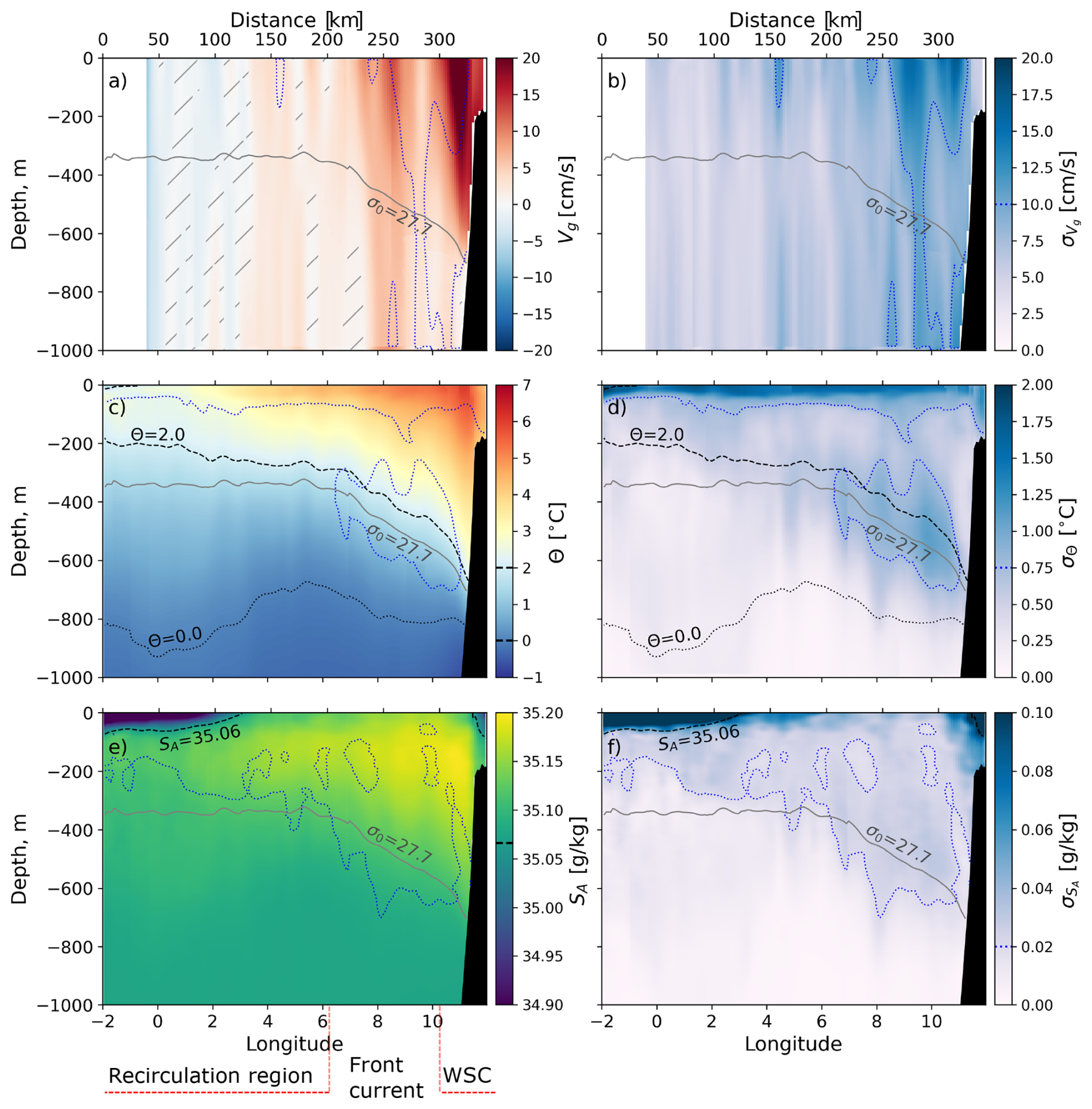
Figure 3 Average (left column) and standard deviation (right column) fields of the (a, b) geostrophic velocity, v_g, (positive northward), (c, d) temperature, Θ, and (e, f) salinity, S_A, based on the 22 glider sections. In (a) absolute velocities less than 1 cm s⁻¹ are hatched. Average contours of σ₀=27.7, Θ=2.0 and 0.0 °C and S_A=35.06 are indicated. Blue dotted contours indicate standard deviation of (a, b) ${\mathit{\sigma }}_{v_{\mathrm{g}}}=\mathrm{10}$ cm s⁻¹, (c, d) σ_Θ=0.75 °C, and (e, f) ${\mathit{\sigma }}_{S_{\mathrm{A}}}=\mathrm{0.02}$. Below panel (e) the regions of Recirculation, Front Current, and the WSC are indicated.

Volume transport of recirculating Atlantic Water (Q_RAW) is calculated in the region west of 200 km. Within the recirculation region we estimate the volume transports of both northward and southward flowing warm water as we expect that warm water flowing northward at these longitudes might eventually recirculate farther north in Fram Strait, and ultimately be brought southward instead of entering the Arctic Ocean (e.g., Hattermann et al., 2016; Hofmann et al., 2021; Wekerle et al., 2017). When presenting estimates of Q_RAW we indicate the northward and southward components separately. The magnitude of the largest of the two estimates may serve as a potential upper limit of the total Q_RAW in the part of Fram Strait covered by the gliders. The same salinity limit as for Atlantic Water is applied, but the temperature threshold is lowered to 0 °C following the water mass classification of RAW by Rudels et al. (2005). The water mass classification and the data selected as RAW are highlighted in Fig. 4a. We do not apply the density limits of σ₀>27.97 for RAW and σ₀>27.7 for AW as this disregards much of the near-surface warm water that is saline enough to be Atlantic Water (Fig. 4). Note that southward flowing Atlantic Water east of 200 km, e.g., due to eddies, is not included in our estimate of recirculating Atlantic Water.

The glider does not always cover the full target section. Consequently, the volume transport of the most eastern and western regions cannot always be estimated directly. To directly compare the volume transport of all the sections, however, the transect area should always be the same. We, therefore, approximate the average AW and RAW volume transport as a function of zonal distance using all the sections. These estimates are then used to fill the missing edges of the sections that do not sample the complete target transect. The average added volume transport is 1.6 % of the total volume transport for the WSC core estimate (east of 300 km), 2.1 % for the Front Current region (200–300 km), and 16.6 % for the Recirculation region (west of 200 km). Sections with no data in the relevant regions are omitted from these estimates. Out of the total 22 sections, two sections had less than 75 % data coverage in the WSC and the Front Current regions while eight sections had less than 75 % data coverage in the Recirculation region.

Some uncertainty in the transport estimates arises from the methodology used to prepare the glider data for analysis. Uncertainties on transport estimates using similar analysis of glider data have been carefully estimated and described earlier (e.g., Kolås et al., 2020, 2024). Their objective mapping, gridding and transport calculations are similar to those presented here. Conservative estimates of the uncertainty in transport calculations of AW in the boundary current north of Svalbard from Seaglider sections were 0.1 to 0.2 Sv (Kolås et al., 2020), and less than 0.1 Sv in the Barents Sea (Kolås et al., 2024). This is much less than the variability quantified by the standard deviation in our results (e.g. Tables 2 and 3, and the shading in Fig. 6) and is typically less than 0.1 standard deviation. Added uncertainties include those arising from filling the missing edges of the sections (quantified above) and those arising from using surface geostrophic currents from the altimeter instead of DAC from the glider (quantified in Sect. 2.2).

3 Results and discussion

In the following we first present the average structure of the observed transect, followed by volume transport estimates of AW and RAW. We next discuss the temporal variability, in particular in relation to wind forcing, and lastly present two case studies of the conditions at the transect during anomalous wind stress conditions.

3.1 The average state

The composite average of the absolute geostrophic velocity, temperature and salinity are presented in Fig. 3, together with their standard deviations over the different occupations. The WSC and the Front Current are both clearly represented in the average velocity sections (Fig. 3a). On average, the WSC is centered over the 1100 m isobath and brings AW northward at a mean velocity of $\mathrm{14.6}\pm \mathrm{9.9}\mathrm{cm}{\mathrm{s}}^{-\mathrm{1}}$. Further west, the Front Current is, on average, positioned between approximately 230 and 280 km, however, its strength, width, and location vary considerably, as indicated by the large standard deviation between the two current cores (Fig. 3a, b). This implies that the two branches are sometimes separated and at other times merged.

Intermittent merging of the current cores makes it difficult to apply an objective and robust method to delineate the cores. A simplified estimate of the WSC core width can be made based on the northward volume transport. We consider the vertically integrated volume transport of each section (i.e., Q as a function of zonal distance) and estimate its maximum value east of 275 km in each section, Q_max. We limit the estimate to the east of 275 km to only select sections with distinct WSC and Front Current cores. We then compute the average northward volume transport across all sections with Q_max greater than the 60th percentile. The zonal extent of the region with transport exceeding this threshold gives a representative estimate of the WSC width, 28± 7 km. The standard deviation is due to variability at the western boundary.

The average temperature and salinity fields illustrate how the warm AW of the WSC closely follow the continental shelf break, where AW reaches depths of approximately 600 m (Fig. 3c, e). The velocity-weighted average temperature (Eq. 1) within the WSC is more than 1 °C warmer than within the Front Current region (4.1 °C vs. 2.8 °C, Fig. 4). The velocity-weighted average salinity is 35.156 g kg⁻¹ within the WSC and 35.146 g kg⁻¹ within the Front Current. While the highest average temperatures occur near the shelf break, waters warmer than 2 °C extend across the entire transect. Still, differences in water mass properties east and west of 200 km are evident in Θ−S_A space: Both the average northward and southward temperature within the Recirculation region is colder than 2 °C, the limit of AW (Fig. 4). In addition to the zonal variability, the standard deviation of the temperature field highlights variability in the vertical extent of the thermocline, allowing for a temporally variable amount of AW past the transect.

Atlantic Water is present throughout all missions but reached a maximum temperature of 9.2 °C in early autumn 2022. The highest salinity, 35.2 g kg⁻¹, was recorded during the subsequent section, while the maximum velocity (60 cm s⁻¹) occurred the previous year, in November 2021. The coldest water masses observed were sufficiently dense to meet the Nordic Seas Deep Water characteristics as defined by Rudels et al. (2005). These water masses were only detected within the WSC and Front Current regions (Fig. 4).

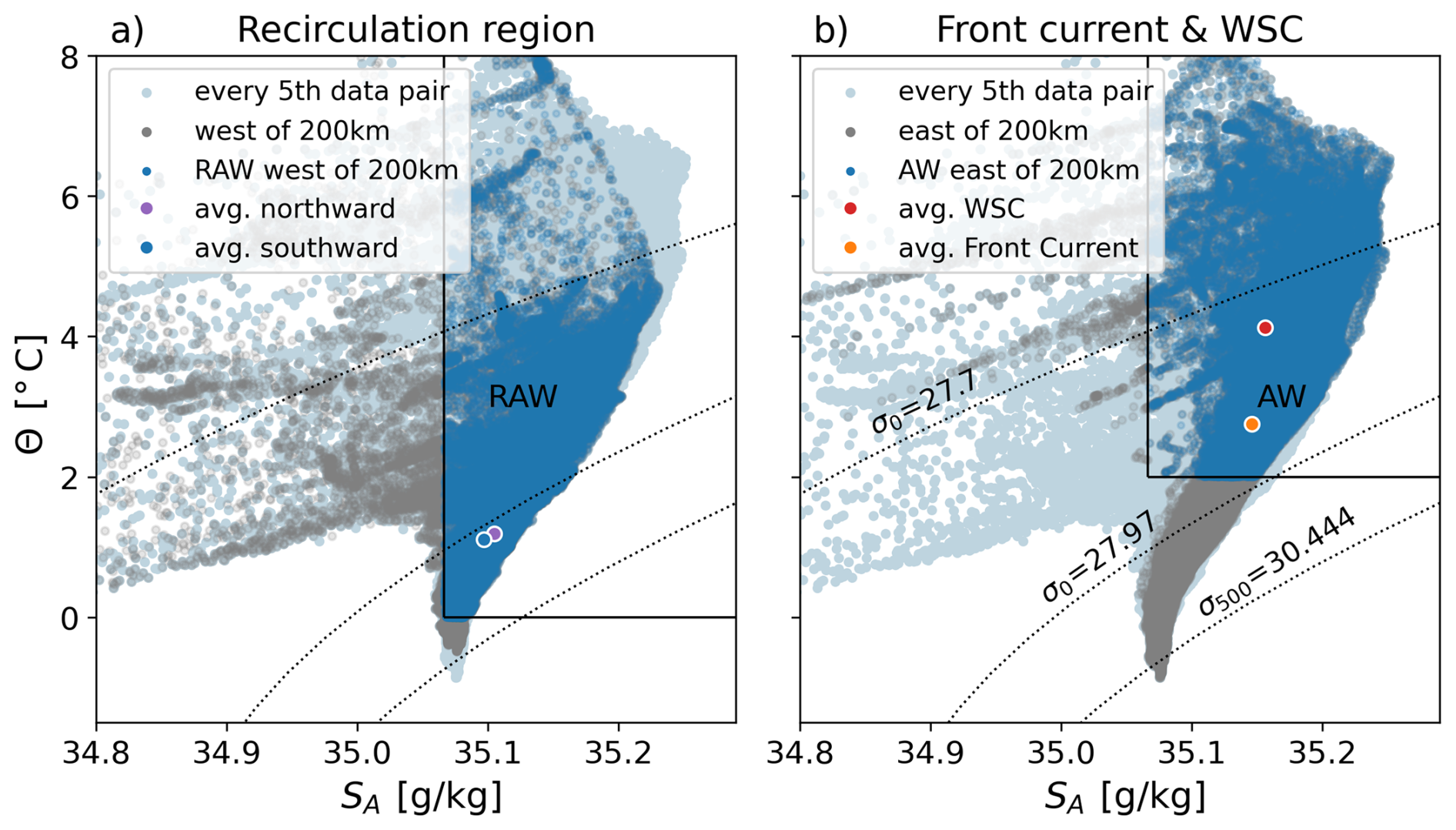
Figure 4 Θ–S_A diagrams for the (a) Recirculation region and (b) the Front Current and WSC, i.e., west and east of 200 km, respectively (grey dots). Temperature and salinity that corresponds to (a) recirculating Atlantic Water (RAW) and (b) Atlantic Water (AW) are highlighted in blue. The light blue markers in the background show the data from the full transect and are the same in both panels for reference. Every fifth data point is shown. Average Θ–S_A values of (a) the Recirculation region within the northward and southward current domains, and (b) within the WSC and Front Current regions are indicated according to the legend.

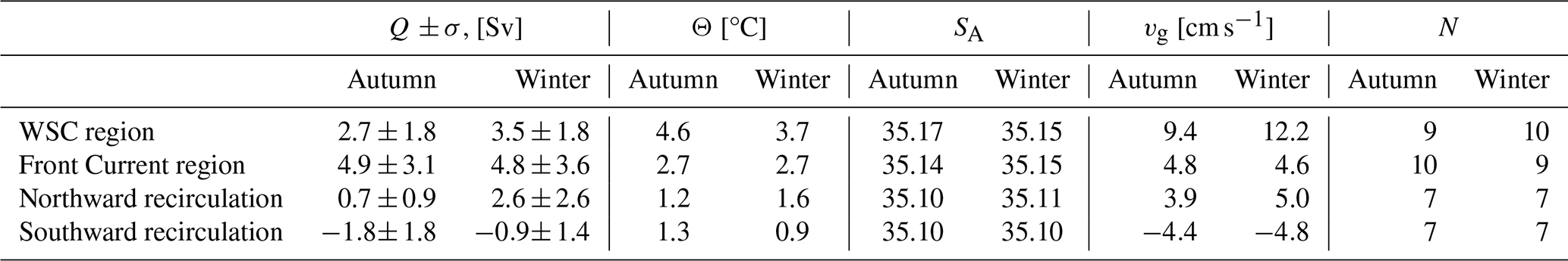
Average properties and volume transports during autumn and winter, computed over the selected branches, are listed in Table 2. These calculations are not constrained by water mass criteria. The WSC is clearly enhanced in winter relative to autumn (12.2 cm s⁻¹ vs. 9.9 cm s⁻¹), in agreement with Beszczynska-Möller et al. (2012). The velocity-weighted mean temperature of the WSC branch, however, decreases from 4.6 °C in autumn to 3.7 °C in winter. In the Front Current, neither the velocity nor the temperatures in winter and autumn are significantly different from each other. In the Recirculation region, the northward transport increases 3 to 4 times in winter relative to autumn, however, both average values are enveloped by equally large standard deviations, highlighting the large variability.

Table 2 Volume transport (Q), velocity-weighted mean temperature (Θ) and salinity (S_A), and mean velocity (v_g) during the glider missions, computed over the selected circulation branches from the average autumn and winter fields. N denotes the number of sections with more than 75 % data coverage included in each average. The total number of sections is 10 for autumn and 11 for winter. Calculations are over the horizontal extent of the branches and the full vertical extent of the measurement, not constrained by water mass criteria. Net values are shown for the WSC and Front Current regions, while the Recirculation region is separated into northward and southward transports. σ is one standard deviation.

3.2 Volume transport: Atlantic Water and recirculation

Net volume transport estimates for AW (in the WSC and Front Current regions) and RAW in the Recirculation region are listed in Table 3 for autumn, winter and the total period. For comparison, the long-term mean (1997–2010) net volume transport of water warmer than 2 °C (same temperature limit as in our analysis) past the full Fram Strait mooring array is 3.0±0.2 Sv (Beszczynska-Möller et al., 2012), with 1.3±0.1 Sv carried in the WSC core.

Transport estimates in temperature–salinity bins, presented in Θ−S_A space, show largest volume transports in the Atlantic Water class between the 27.7 and 27.97 isopycnals (Fig. 5c). As the barotropic component generally dominates the northward current (Fig. A2), there is also a substantial northward transport of the deeper cold and denser water masses (Figs. 5c and A3). There is a clear distinction in water mass density classes transported by the WSC and the Front Current (Fig. A3). The WSC transports a relatively broad density range centered around ${\mathit{\sigma }}_{\mathrm{0}}=\mathrm{27.75}\mathrm{kg}{\mathrm{m}}^{-\mathrm{3}}$, while the Front Current carries denser waters characterized by two narrow peaks: one centered at approximately σ₀=27.9, and one at ${\mathit{\sigma }}_{\mathrm{0}}=\mathrm{28.05}\mathrm{kg}{\mathrm{m}}^{-\mathrm{3}}$. This is a manifestation of the different water mass modifications the slope and front branches of the Norwegian Atlantic Current experience as they move poleward. Huang et al. (2023) showed that in the mean state from 2005 to 2018, air-sea heat flux accounts almost entirely for the net cooling of AW along the Front Current, while oceanic lateral heat transfer appears to dominate the temperature change along the Slope Current. At approximately 77° N, before the two branches merge in Fram Strait, the average density of the Slope Current is about 27.8 whereas the Front Current is 27.9 kg m⁻³ (their Fig. 2e). Similarly, Walczowski (2013) presents the 1996–2007 summer mean transect along 76°30^′ N (his transect “N” and Fig. 5.6), at a location before the different branches converge. Two zones of baroclinicity and resulting baroclinic currents are clearly distinct: above the Knipovich Ridge (the Front Current) and above the Spitsbergen slope (the WSC core), with the front branch approximately 0.1 to 0.15 kg m⁻³ denser. Our observations are thus consistent with these analyses.

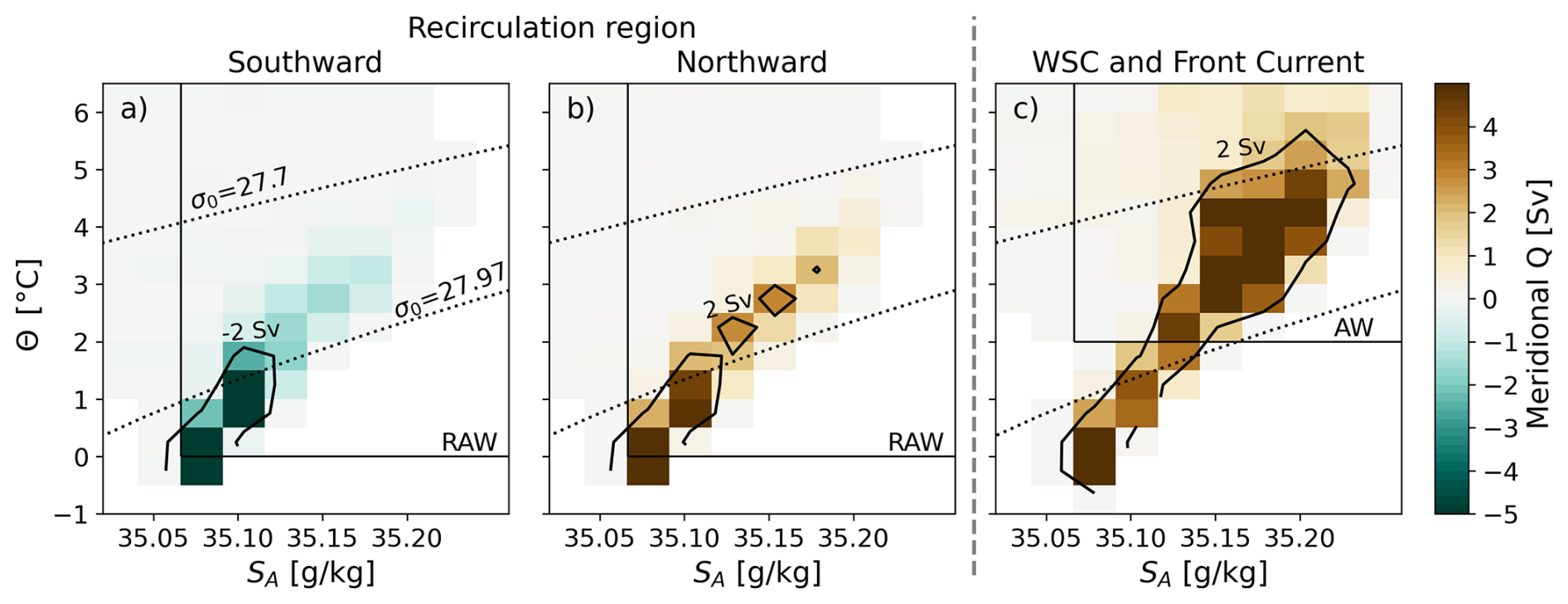
Figure 5 Volume transport in Θ−S_A space for (a) southward and (b) northward velocities in the Recirculation region west of 200 km, and (c) the full velocity field east of 200 km covering WSC and the Front Current. Vertical and horizontal black lines indicate salinity and temperature limits for RAW in (a), (b) and AW in (c). The black contours indicate volume transport of 2 Sv (a) southward and (b) northward in the Recirculation region, and (c) net in the WSC and Front Current region.

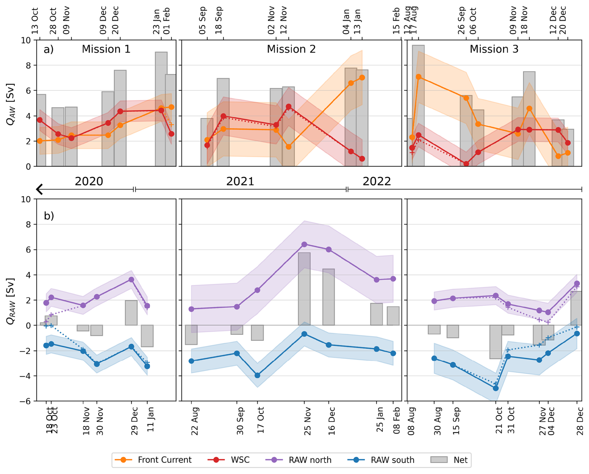
Figure 6 Volume transport, Q, of (a) northward Atlantic Water (AW) and (b) Recirculating Atlantic Water (RAW) separated into (a) northward Q_AW within the WSC (red) and the Front Current (orange) and (b) northward (purple) and southward (blue) Q_RAW. Grey bars indicate total transport in each panel. Colored shading represents the standard deviation of the transports. Dates correspond to the temporal midpoint of the glider's transit across each domain (east of 200 km for AW and west of 200 km for RAW). Sections not fully sampled by the glider are extrapolated using the average volume transport, except section 14 for Q_AW and sections 7 and 15 for Q_RAW, which are omitted due to missing data in the eastern and western domains, respectively. Estimates without extrapolation are shown as dotted lines in the respective colors. Note that the x-axes of the two rows align, although the time labels differ, and that there is five to six months gap between missions.

Table 3 Volume transport (Q) during the average autumn, winter, and total average fields constrained by water mass criteria. Section nr 14 is not included in the total estimate since it lasted from 7 to 15 August, which is not categorized as winter or autumn. Net values are shown for the WSC and Front Current regions, while the Recirculation region is separated into northward and southward transports. σ is one standard deviation.

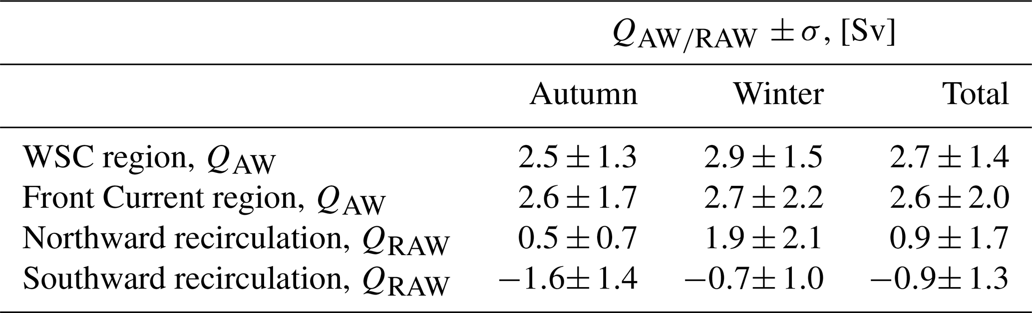
West of 200 km, in the region of recirculation, there is relatively strong average volume transport of RAW both northward (0.9 Sv) and southward (−0.9 Sv, Table 3). This could amount to a total recirculation of 0.9 Sv assuming that the northward flowing RAW within the defined recirculation region follows the recirculation branch at about 78° N (Hattermann et al., 2016; Hofmann et al., 2021), veering westward and ultimately flowing south, captured again at the western part of our glider transect.

Assuming our limited observations are representative for a longer-term average, the large difference between our estimates of total Q_AW (WSC region and Front Current region: $\mathrm{2.7}\mathrm{Sv}+\mathrm{2.6}\mathrm{Sv}=\mathrm{5.3}$ Sv) and the mooring-based transport (3 Sv, Beszczynska-Möller et al., 2012), further implies that approximately 2 Sv of AW must have been lost to recirculation between 77°15^′ and 79° N. This agrees with the recirculation estimate by Marnela et al. (2013). A fraction of the discrepancy could also be due to high-resolution measurements from gliders resolving the branches better relative to the mooring array.

The discrepancy between the glider-based estimate of 0.9 Sv southward RAW and the potential 2 Sv of AW lost to recirculation between 77°15^′ and 79° N might be due to the limited westward extent of the glider sections. At the latitudes of our target section, eddy-resolving model studies locate the equatorward limb of the southern recirculation branch between 0–3° W, near the 3000 m isobath, and of the northern recirculation branch between 3–5° W, near the 2000 m isobath (Wekerle et al., 2017, e.g., their Fig. 7). It is therefore likely that the glider sections do not capture the full southward recirculation as the glider often had to turn west of the Prime Meridian because of sea ice in the region. Since the glider target section was at 77°15^′, i.e., upstream of where the Front Current and the WSC tend to merge and south of where the northern recirculation branch is expected to diverge from the slope current (Hattermann et al., 2016; Wekerle et al., 2017), it is also likely that our northward recirculation transport is an underestimate.

While the northward and southward recirculation transports nearly balance for most sections (Table 3, Fig. 6b), the properties of the waters they carry differ markedly (Fig. 5a, b). This indicates that these transport components are not isolated eddies or other reversible flow across the glider transect. The northward transport is warmer and more saline than the southward transport (Fig. 5a, b). This change in water mass properties suggests a coherent recirculation pattern, where relatively warm northward-flowing waters are modified during their southward return, cooling and mixing with colder, fresher waters along the path.

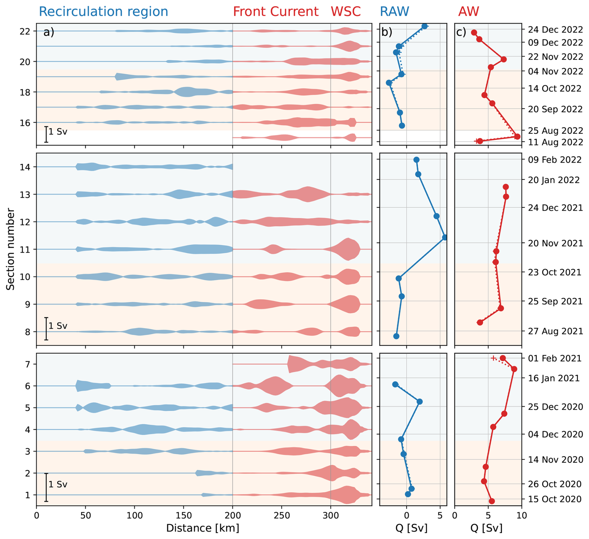
Figure 7 The volume transport of net recirculating Atlantic Water (Q_RAW, blue) and northward-flowing Atlantic Water (Q_AW, red). (a) The zonal variability of Q_RAW west of 200 km (blue) and Q_AW east of 200 km (red) for each section in 2 km binned averages. The volume transport is mirrored over the horizontal axis to emphasize the zonal variability. A scale of volume transport is indicated in the lower left corner of each row. The scales differ because the height of the panels is determined by the total duration of the mission, not the number of sections during the mission. The zonally summed (b) net Q_RAW and (c) northward Q_AW with (solid) and without (dotted) extrapolation of unsampled regions. The dates along the vertical axis of panel (c) are the temporal midpoints of each section. Autumn and winter are indicated by the blue and orange background shading.

3.3 Temporal variability of volume transport

Gliders traversed the target section repeatedly over three years, and offer some insight on seasonal and interannual patterns. Note that the full seasonal cycle cannot be resolved as the gliders mostly sampled autumn and winter, and lack sections in spring and summer.

During 2020 and 2022 there appears to be systematically higher transport of AW within the WSC during winter than autumn (Fig. 6). This seasonality agrees with the seasonality within the offshore WSC branch observed in Beszczynska-Möller et al. (2012), but disagrees with the lack of seasonality within their main WSC core. This partial agreement could be fortuitous and due to lateral adjustments in current characteristics or interannual variability. For example, during mission 2, the AW transport in the WSC was relatively high during both crossings in autumn, and low in January.

While the mean net transport of the WSC and Front Current are comparable (within 0.1 standard deviation, Table 3), some sections have significantly larger near-instantaneous northward Q_AW in the Front Current, e.g. in January 2022 and the second half of August to September 2022 (∼2 times the average, Fig. 6a). The lack of seasonal variability within the core defined by Beszczynska-Möller et al. (2012) implies that the near-zero Q_AW estimates within the WSC in our data (e.g., January and September 2022) likely occur because the core is displaced out of the zone selected for this branch and potentially merged with the Front Current, or temporarily suppressed. Figure 7 complements the overview presented in Fig. 6 of volume transport estimated per branch and section, and illustrates the distribution of volume transport across the transect for each section, highlighting variability in the position of the circulation cores. The tendency of higher Q_AW in the Front Current when it is weaker in the WSC, supports that displacement but not suppression is the reason for the low WSC transport (Fig. 6a).

A reduced amount of water warm and saline enough to be considered AW could also explain the sections of low AW volume transport. However, the area of AW present in the WSC region remains relatively stable throughout the glider sections and there is no correlation with Q_AW (R²=0.01, excluding section nr 14 as it did not cover the WSC and Front Current regions). Conversely, in the Front Current region, the cross-sectional area of AW does co-vary with the AW volume transport (R²=0.7, excluding section nr 14). This suggests that the volume of AW limits Q_AW in the Front Current region but not in the WSC region. The current speed is thus the remaining factor that can control the AW transport in the WSC region. If this is the case, we would expect a large AW area to yield high Q_AW in the Front Current but not in the WSC unless the currents are also strong. Two examples with anomalously weak Q_AW in the WSC but large Q_AW in the Front Current are sections 12 and 13 (Figs. 6a and 7a). During these sections, the σ₀=27.97 isopycnal is deep and relatively flat (630 ± 50 and 600 ± 95 m compared to 490 ± 120 and 380 ± 95 m for the case study sections 9 and 22 discussed below), sustaining a large volume of AW in both the Front Current and WSC regions. However, the average WSC velocities are low (section 12: 5 cm s⁻¹ and section 13: 2 cm s⁻¹), and the large cross-sectional area of warm water thus does not translate into high Q_AW in the WSC.

While the divide between the Front Current and WSC regions at 300 km appears to be a robust choice (Figs. 3 and 7), these two current cores do occasionally merge (e.g., sections 2, 5, 12) and shift (e.g., sections 13 and 17, Fig. 7). This contributes to the apparent fluctuation between strong Q_AW in the Front Current and the WSC during some instances. We thus note that a larger sample size would be necessary to make a more confident conclusion regarding the possible distinction in limiting factors of Q_AW (area of AW vs. current speed) in the WSC and the Front Current.

In the Recirculation region there is a tendency for co-variability between the northward and southward transports (Fig. 6b). This indicates that the region is either dominated by northward current or southward current, rather than separated into two segments with northward flow furthest east and southward in the west. Limited to only 7–8 data points with irregular temporal spacing per mission, we cannot confidently quantify the amplitude and lag of co-variability. For most sections, the net volume transport of RAW is directed southward (Fig. 6b). Considering observed and modeled mean circulation in this region (e.g., Hattermann et al., 2016; Beszczynska-Möller et al., 2012; Wekerle et al., 2017; Hofmann et al., 2021) where the main recirculation occurs west of 0° E, it is surprising that the southward component dominates as far east as in our defined Recirculation region (∼0°–6° E). The main exception is in November and December 2021, when there is a strong (>4 Sv) northward transport of RAW also in the Recirculation region. This variability in direction of the RAW transport is likely not influenced by the position of the Front Current, as its average position and region of high standard deviation are well away from the boundary between the Recirculation and Front Current regions (Fig. 3a, b). It thus indicates relatively large variability in the circulation pattern between the northward AW branches and the southward East Greenland Current.

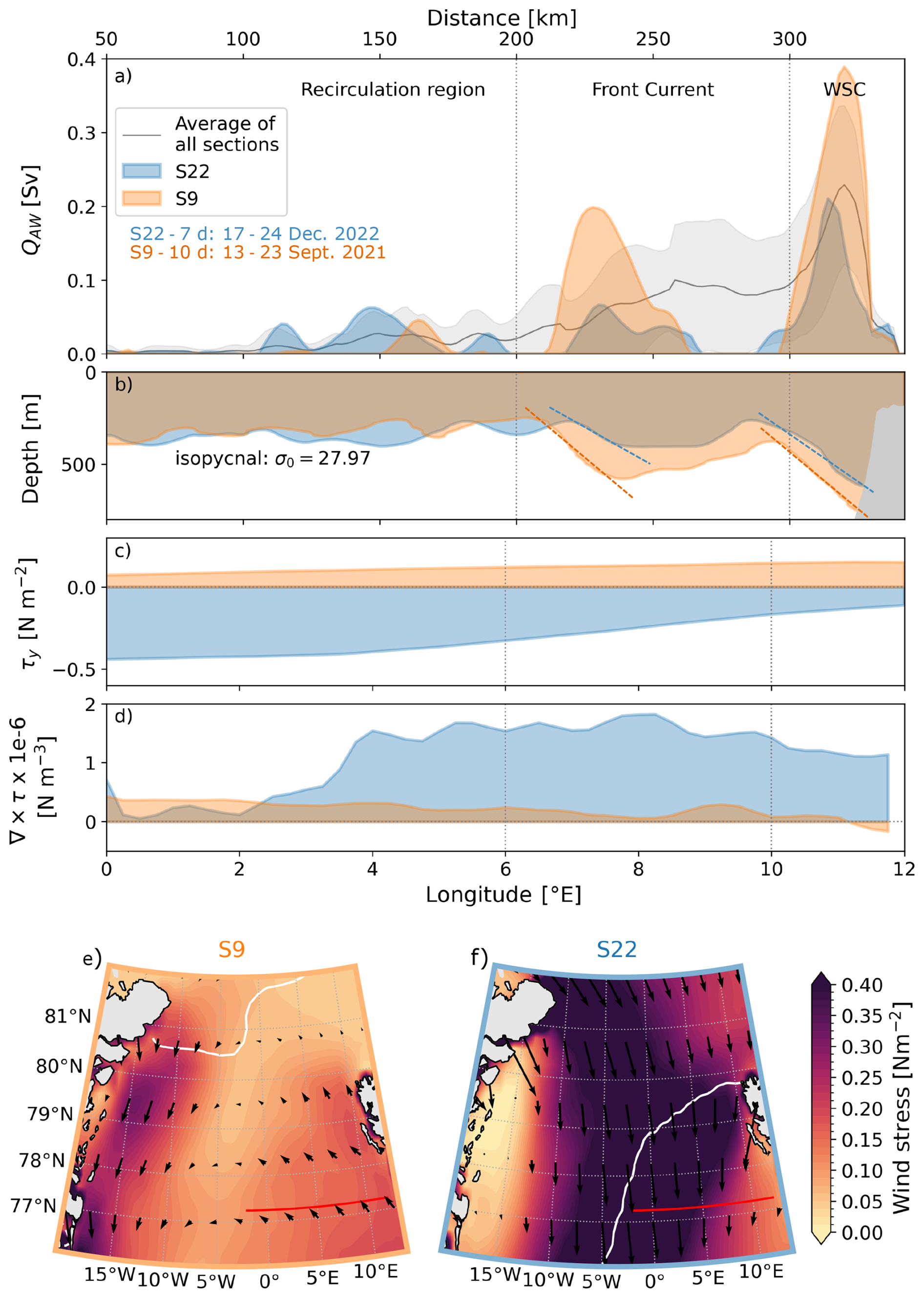
Figure 8 (a) Northward Q_AW in 2 km binned averages and (b) the σ₀=27.97 isopycnal depth of glider sections 9 (S9, orange) and 22 (S22, blue). The gray line and shading in panel (a) are the average and standard deviation over all sections. The colored dashed lines in panel (b) indicate the slopes of the fronts supporting the WSC and the Front Current. Average (c) meridional wind stress and (d) wind stress curl over 77.25° N±0.75° and the full wind stress field for (e) section 9 and (f) section 22 during the time it took the glider to cross the distance spanning from 200 km on the target transect to the eastern boundary for sections 9 and 22. White contour is the sea ice edge and the red line is the target transect.

3.4 Case study: Atmospheric forcing of Q_AW variability

To investigate potential drivers of the variability in Q_AW, we identify two sections of distinctly different wind stress forcing over the glider transect: September 2021 (case S9) and December 2022 (case S22, Fig. 8). During September 2021, the wind stress was anomalously strong northward and aligned with the shelf break, while during December 2022, the wind stress was anomalously strong southward (compared to conditions during the glider deployment periods). We expect that the effect of wind stress on the WSC through coastal Ekman transport can happen quickly (< day). The response time is likely longer (day to week) for the effect of Ekman pumping/lifting of the isopycnals supporting the Front Current. In comparison, the average duration to cover the WSC and Front Current region is 9 d, and the WSC region alone is approximately 3 d. During the case studies, the wind field is averaged over 7 (S22) and 10 d (S9).

The wind stress conditions during these two cases are not rare in a long-term perspective (Fig. A4). An analysis of wind stress extracted from ERA5 during 1979–2024 and averaged over our analysis section within 7 d-long overlapping windows shows that northward wind stress values exceeding the maximum during case S9 occur 2–15 times each year. Similarly, values of southward wind stress stronger than the maximum southward stress during case S22 occur 1–12 times each year. The maximum stress values during the two case studies are within the 5th and 95th percentiles of the maximum absolute wind stress for each 7 d-long window between 1979 and 2024 (Fig. A4b). The cases highlighted are thus not extreme conditions in terms of maximum wind stress but represent atmospheric forcing that may be expected to occur several times each year.

Unlike the wind stress, while the September 2021 case (S9) was within the typical expected values of wind stress curl (horizontally averaged over the Front Current and WSC regions: 6–12 °E, 77.25° N±0.75°), the average wind stress curl during section 22 in December 2022 was stronger than the 95th percentile (Fig. A4c).

During case S22 when southward wind stress dominates, the WSC is relatively weak and the outer core is nearly disintegrated (Fig. 8a, blue). This reduced WSC strength might be a direct result of the anomalous wind stress through positive zonal gradients (Fig. 8c, d) and resulting Ekman transport away from the coast which (i) lifts and flattens the isopycnals reducing the baroclinic current component, and (ii) reduces the sea surface anomaly towards the coast which reduces the barotropic current component. The reduced AW volume transport in the Front Current region during southward stress might be related to open-ocean divergence in the Ekman layer. Just as over the WSC region, the zonal gradient in the meridional wind stress is strongly positive over the Front Current (Fig. 8c, d). The average wind stress over the WSC is roughly $-\mathrm{0.15}\mathrm{N}{\mathrm{m}}^{-\mathrm{2}}$ and the maximum southward wind stress further east is 0.4 N m⁻², causing a wind stress curl of almost $\mathrm{2}\times {\mathrm{10}}^{-\mathrm{6}}\mathrm{N}{\mathrm{m}}^{-\mathrm{3}}$. The resulting divergence might have caused anomalously strong lifting and flattening of the isopycnals that support the Front Current, consequently slowing down the current. While limited in sample size by 22 sections, a more robust conclusion can be attempted based on a composite analysis using sections with weak Front Current transport. We select the sections with Q_AW, max within the Front Current less than its 10th percentile over all sections. The average wind stress field during these three sections has a dominant southward component (not shown), supporting a relationship between the southward wind stress and the Front Current strength. Note that the significance of this composite is limited by the sample size of three out of 22 sections.

During the northward wind stress anomaly, in case S9, the maximum AW volume transport within the WSC is nearly twice as strong as the average (Fig. 8a, orange vs. gray). There is also a clear core within the Front Current region, and these two current cores are distinctly separated. The northwestward wind stress likely heightens the sea surface along the coast and steepens the isopycnals, driving both an enhanced northward barotropic and baroclinic current component. Similarly to cases of weak Front Current transport, a composite can be made of the wind stress field during strong WSC transport. We detect three sections when Q_AW, max in the WSC was larger than its 90th percentile over all sections. The average wind stress field during these three sections has a clear northwestward component (not shown). Conversely, the wind stress curl during case S9 was nearly zero, thus yielding minimal impact on the deep isopycnals. In agreement with this weak wind stress curl, the 27.97 kg m⁻³ isopycnal is steeper in both the Front Current and the WSC regions during case S9 when the volume transport is strongest (Fig. 8b). This suggests that the observed difference in AW volume transport is at least partly baroclinically driven.

Frank et al. (2025) investigated warm AW intrusions onto the West Spitsbergen Shelf as identified from high-resolution regional model output across zonal cross-shelf sections starting from 77°20^′ N, close to our target section. The amplitudes of WSC velocity peaks appear to be reduced during prolonged periods of strong offshore Ekman transport, and the current tends to be positioned further offshore over deeper bathymetry – similar to our case S22. They emphasize that events of on-shelf AW intrusion were influenced by multiple cross-shelf exchange mechanisms that may act simultaneously (e.g., increase in core speed, displacement of core on the slope, near-surface onshore Ekman transport of warm water, upwelling of deeper waters in response to offshore Ekman transport etc.). Similarly, we could expect multiple processes leading to variability in the relative position, strength and interactions of the Front Current and the WSC.

4 Conclusions

We present transport estimates of warm Atlantic Water (AW) and Recirculating Atlantic Water (RAW) across a zonal transect at 77°15^′ N based on repeated ocean glider sections. In total, 22 sections were collected during three missions covering autumn and winter in 2020, 2021 and 2022. The fine spatial resolution of the glider transects provides well-resolved circulation cores, lending confidence to the estimated volume transports. Although glider data require more extensive post-processing compared to mooring or ship-based observations, their high spatial resolution offers an advantage over traditional mooring arrays, and repeated seasonal coverage provides an improvement over single ship-based sections.

On average, the WSC and the Front Current each transports approximately 2.5 Sv of AW (Θ>2 °C, $S_{\mathrm{A}}>\mathrm{35.06}\mathrm{g}{\mathrm{kg}}^{-\mathrm{1}}$) northward during autumn and winter, resulting in a combined transport of about 5 Sv toward the Arctic. There is an indication of higher AW transport in the WSC during winter compared to autumn, but this difference is not significant within one standard deviation. Additional missions would be required to confirm this apparent seasonality. The elevated winter transport in the WSC coincides with stronger current speeds. Within the Front Current, high AW volume transport also co-varies with the cross-sectional area of warm AW, whereas this is not the case in the WSC region. This suggests that AW availability is a limiting factor for the Front Current but not in the WSC during autumn and winter.

Two cases of anomalous surface wind stress are examined. During the event with strong northward stress over the WSC and Front Current regions, northward transport of warm Atlantic Water is enhanced: both the maximum Q_AW in the WSC and the Front Current are approximately twice their respective average values. This is consistent with the expected Ekman dynamics, where northward wind stress west of Svalbard elevates sea surface height along the coast and strengthens northward barotropic currents. Conversely, during the event with a strong southward wind stress, the WSC weakens and the Front Current nearly disintegrates. During this period, the wind stress curl is positive, suggesting that both lifting of isopycnals and reduced sea surface height anomalies likely contribute to the weakened currents.

Our target section partly captured the southern, weaker recirculation branch in Fram Strait. The net volume transport of RAW (Θ>0 °C, $S_{\mathrm{A}}>\mathrm{35.06}\mathrm{g}{\mathrm{kg}}^{-\mathrm{1}}$) west of the Front Current is close to zero, i.e., the northward and southward average transports approximately balance. However, the properties of the waters they carry indicate a coherent recirculation pattern, where relatively warm northward-flowing waters are modified during their southward return, cooling and mixing with colder, fresher waters along the path. Under this assumption, we estimate the strength of the recirculation at the observed section to be approximately 1 Sv.

This study demonstrates the capability of ocean gliders as observing platforms – even in regions of strong boundary currents. The pronounced variability in the strength, structure, and position of both the WSC and the Front Current could not be captured by a traditional mooring array. This variability appears to reflect atmospheric conditions; however, because the strongest wind stress typically occurs in spring and summer, i.e., between the glider deployments presented here, we cannot assess the most anomalous Q_AW conditions. A mission program extending through summer as well as winter would provide critical insight into current core dynamics and Q_AW under such atmospheric forcing, particularly for the Front Current, which is not constrained by the continental shelf break.

Appendix A: Supporting figures

The depth-averaged currents (DAC) estimated by the gliders agree with the currents we expect from this region for most of the missions, except for roughly the first half of mission 2. Sections 7–10 collected during mission 2 have strong northward DAC estimates ($>\mathrm{10}\mathrm{cm}{\mathrm{s}}^{-\mathrm{1}}$) across the full extent of the section (Fig. A1b). We compared the DAC estimates to surface geostrophic currents from gridded altimeter product (Global Ocean Gridded L4 Sea Surface Heights And Derived Variables Reprocessed 1993 Ongoing, 2024) and concluded that these two estimates compare well except in the period with anomalously high velocities during mission 2 (Fig. A1). While we could not identify the cause, we suspect DAC estimates are erroneous. We therefore use the altimetry based surface geostrophic currents instead of the depth-averaged currents from the glider in our estimates of absolute geostrophic currents for all sections for consistency.

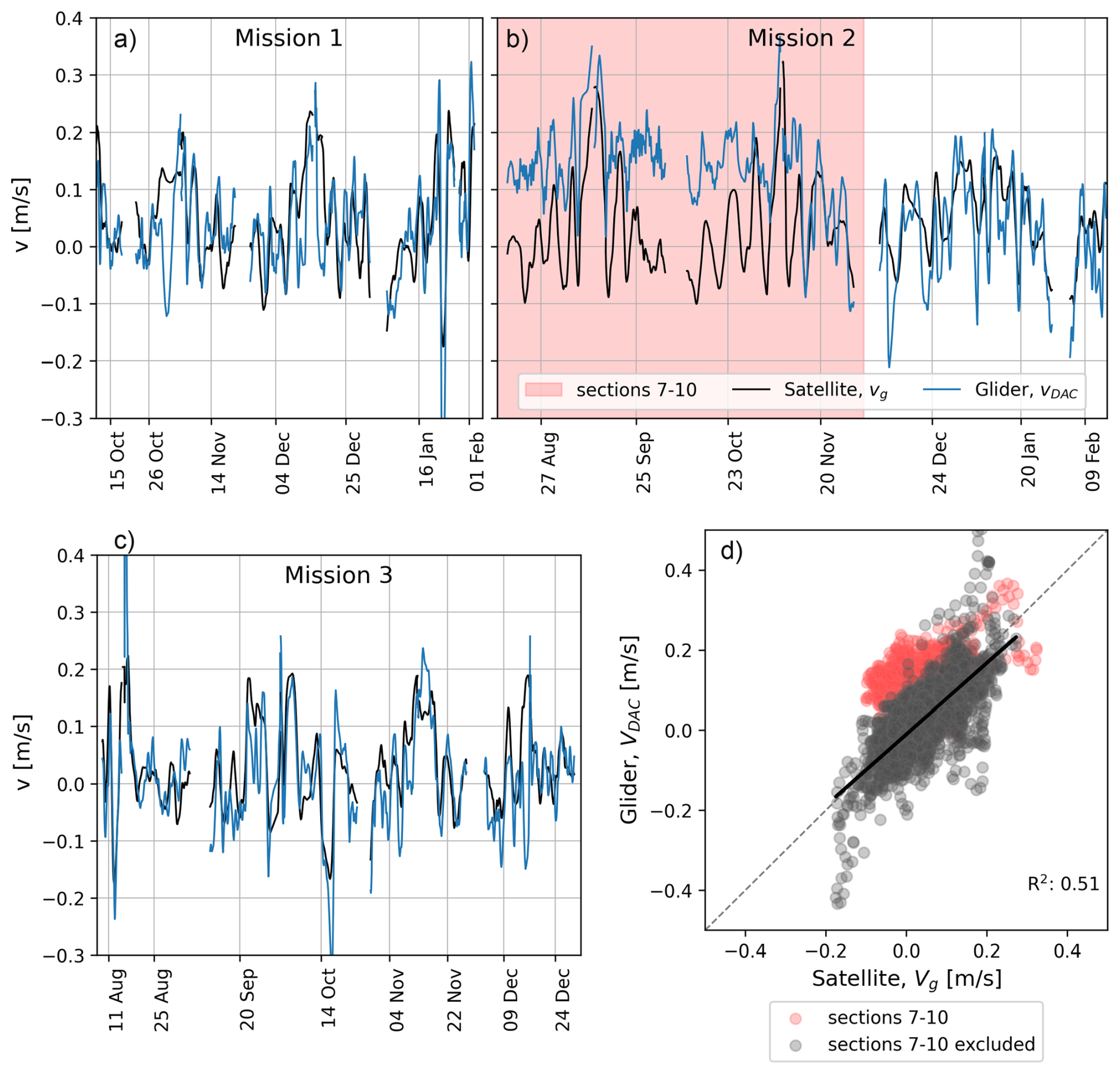
Figure A1 (a–c) Time series and (d) scatter plot of the northward surface geostrophic current (Satellite, v_g) versus the northward component of the depth-averaged current (DAC) between dives estimated by the gliders (Glider, v_DAC). In (b), (d) the pale red region and markers indicate sections seven through ten where v_DAC was suspiciously strong over large parts of the target section. The value of R² in (d) is estimated based on data points excluding sections seven through ten, and the dashed grey line indicates the perfect agreement for reference.

The barotropic and baroclinic current components can be approximated as the depth-averaged current and as the depth-averaged current subtracted from the full current field, respectively (Fig. A2). The velocities are consistently higher in the approximated barotropic component than in the baroclinic component when considering the velocity field averaged over all 22 glider sections (Fig. A2). The same is true for nearly all periods both spatially and temporally when considering each section individually (not shown).

The different regions (WSC, Front Current and Recirculation) carry different water masses across the transect. Both the WSC and the Front Current have a net northward transport within all density classes, including the densest registered water masses (Fig. A3). The WSC brings the lightest AW northward: its distribution peaks at roughly σ₀=27.75, while the Front Current brings denser AW northward, peaking at almost σ₀=27.90 (Fig. A3). Both within the Front Current and the Recirculation region there is a distinct maximum in the densest water mass, with approximately σ₀=28.05 (Fig. A3) and Θ=0 °C (Fig. 5). A small negative value indicates net southward volume transport in the Recirculation region at approximately σ₀=28.0.

In a long-term perspective, the wind stress conditions during the glider missions, and the two case studies (S9 and S22 specifically) were relatively common. Based on wind stress from ERA5 averaged from 1979 to 2024 and in the region 77.25° N±0.75° and 0–12° E, similar conditions are expected several times each year (Fig A4). While there is a substantial seasonal cycle in the wind stress, the distributions of magnitude of maximum and minimum wind stress across the target section are similar, both for the full year (not shown) and for the period August to February (Fig. A4b), covering the glider missions. The wind stress curl is extreme during our case study S22, and is likely representative of the conditions during maximum Ekman lifting.

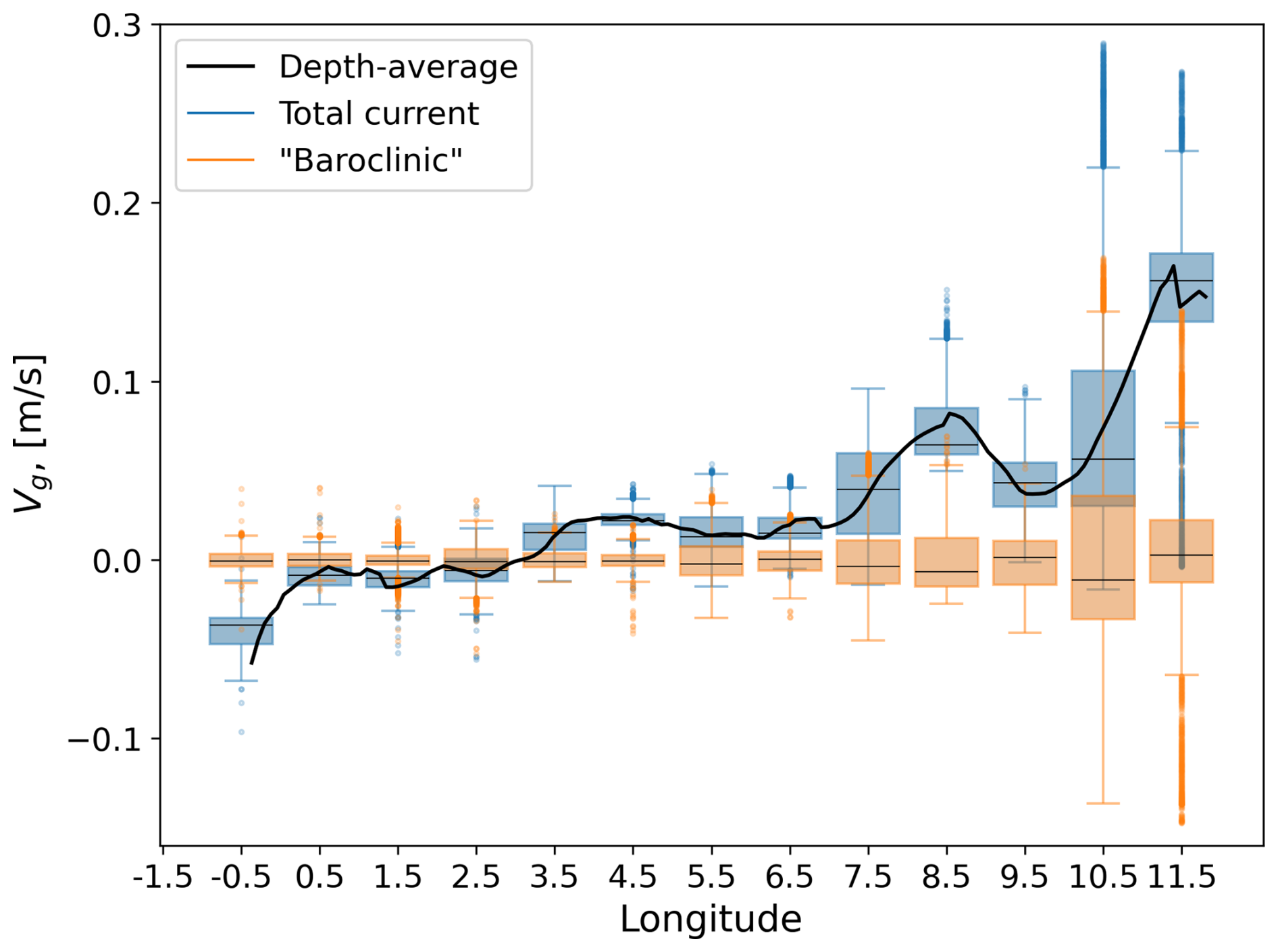
Figure A2 Average current across the target section based on all 22 glider sections. The depth-averaged current (black) and box plots of the depth-varying total current (blue) and the approximated baroclinic current component (total current minus the depth average, orange) in 1° longitude bins. The median of each bin is indicated by horizontal black lines, the box indicates the quartiles, the whiskers indicate the remaining distribution, and the dots are outliers as defined by Seaborn's boxplot function (Waskom, 2021).

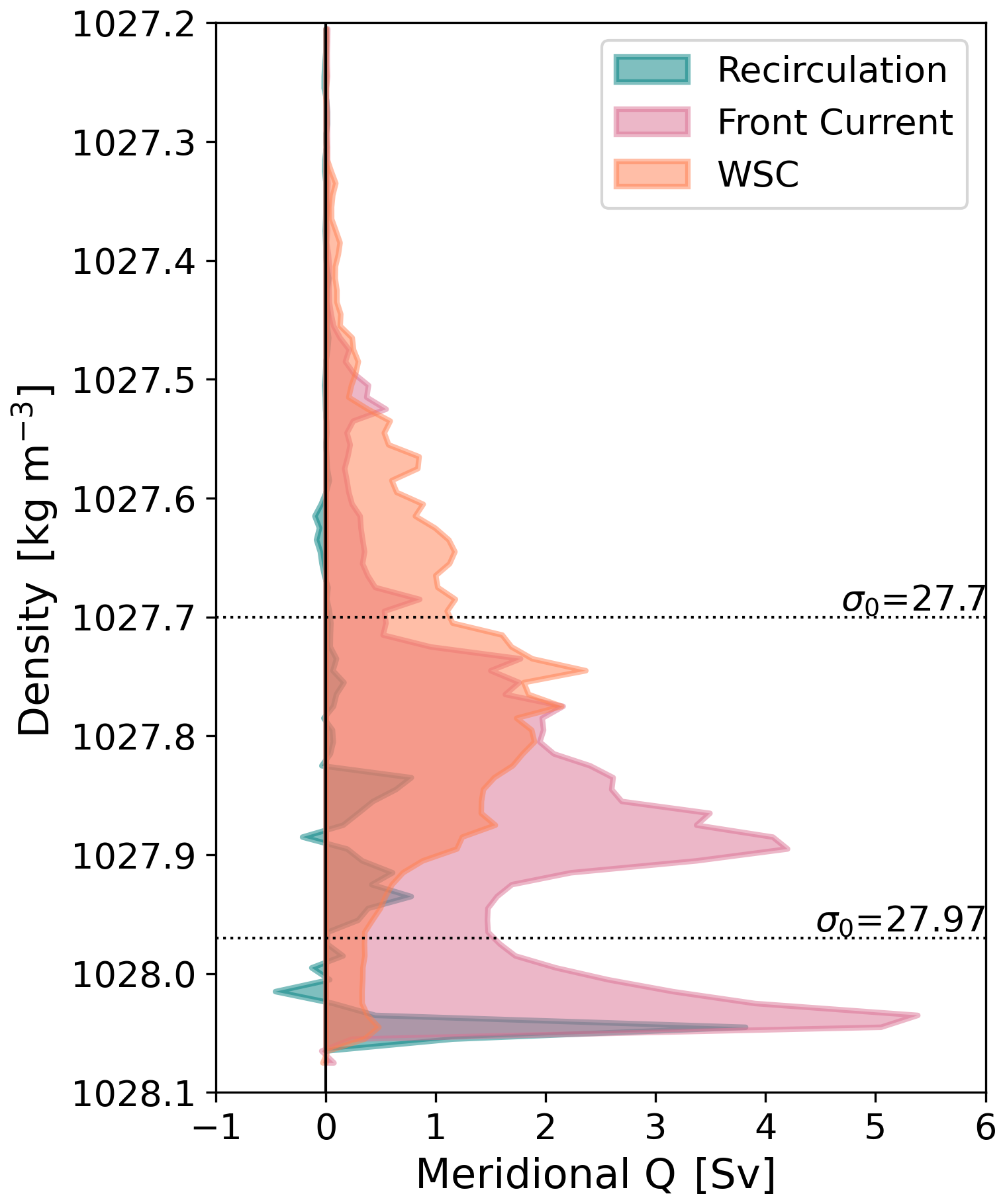
Figure A3 Meridional volume transport as a function of potential density classes for the Recirculation region (teal), the Front Current region (pink), and the WSC region (orange). Selected σ₀ values are indicated.

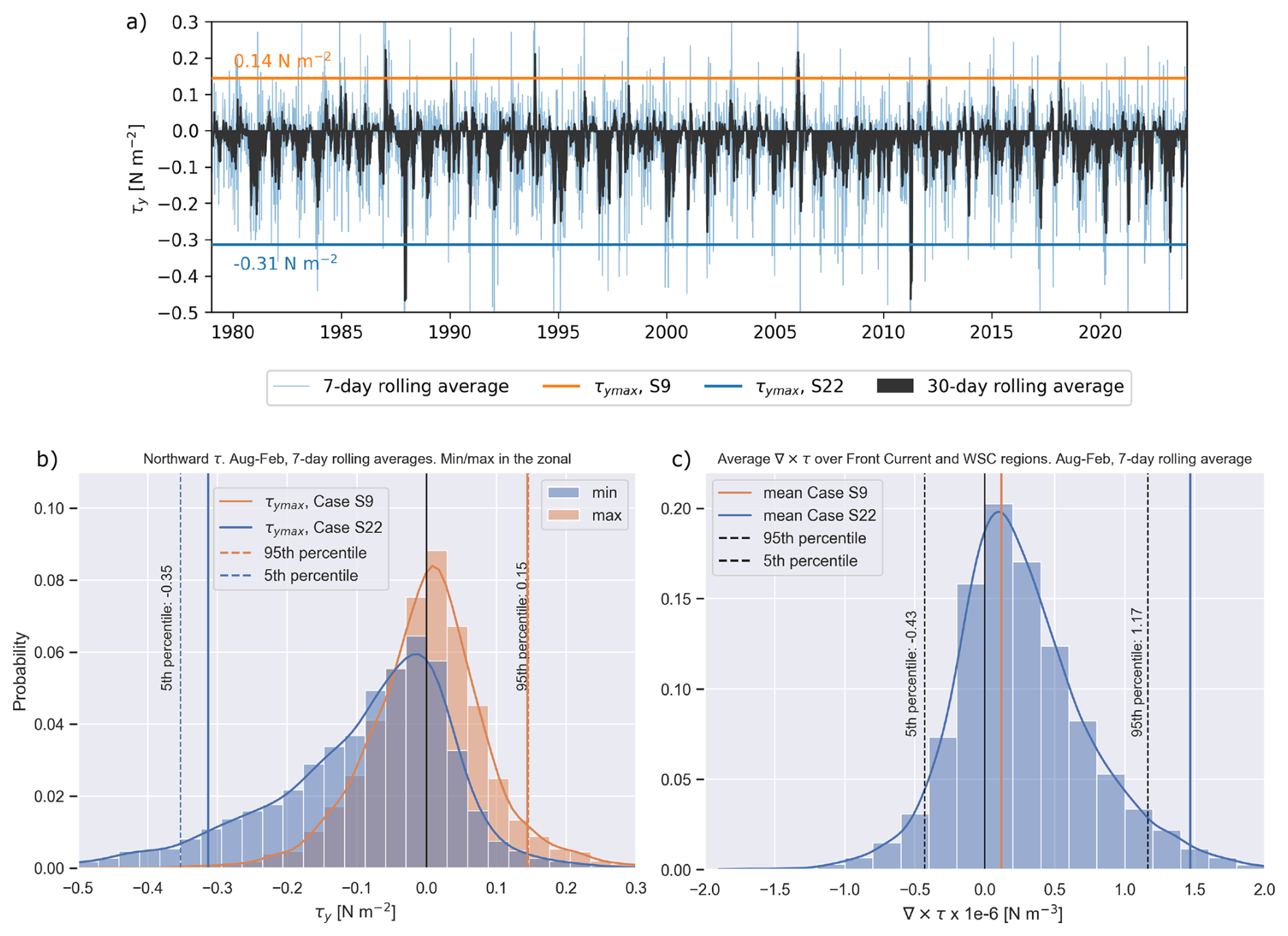
Figure A4 Meridional wind stress (1979–2024) averaged over 77.25° N±0.75° and 0–12° E. (a) Time series of 7 d (light blue) and 30 d rolling averages (dark grey). The maximum wind stress amplitude during sections 9 (orange) and 22 (blue) based on the 7 d rolling average are indicated by horizontal lines. Panels (b) and (c) are both based on the 7 d rolling averages from August to February, the typical coverage of glider missions. (b) Histogram of the zonal maximum northward (orange) and maximum southward (blue) wind stress. Vertical dashed lines show the 5th percentile of the southward stress (blue) and 95th percentile of the northward stress (orange). Vertical solid lines show the maximum amplitudes during the two case studies as in panel (a). (c) Histogram of the wind stress curl over the Front Current and WSC region. The mean wind stress curl during cases S9 (orange) and S22 (blue) are shown in vertical lines. The 5th and 95th percentiles are indicated in vertical dashed black lines.