Quantification of Baltic sea water budget components using dynamic topography

Accurate quantification of the Baltic Sea's dynamics and water budget components is essential for understanding both seasonal and long-term variations influenced by climate change. In this study, we utilize dynamic topography (DT), referenced to a geoid-based chart datum, to derive dynamic water volume and to improve estimates of the main water balance components, such as river runoff and water exchange through the Danish Straits. We utilize DT for the period from 2017 to mid-2021, which was corrected for vertical sea level biases and whose vertical datum thus coincides with the geoid. Our findings reveal seasonal dynamic volume variations, with a minimum in spring (78.9 ± 60 km³) and a maximum in autumn and winter (121 ± 57 and 124 ± 80 km³, respectively). Anomalies in DT highlight a specific region (northern Baltic Proper) as representing equilibrium mean DT for the entire Baltic Sea, while areas in the eastern and southern Baltic are prone to extremes. Barotropic exchange analysis shows that no major Baltic inflows occurred during the study period, with small to medium inflows averaging 1.6 km³ d⁻¹ in autumn and winter, while outflows averaged 2.36 km³ d⁻¹. River discharge, indirectly calculated from the water budget, peaked in summer (2.08 km³ d⁻¹) and was lowest in autumn (1.26 km³ d⁻¹), with hydrological models underestimating flows in these seasons. As a result, the method and results show great potential for quantification, validation, and a better understanding of the dynamics of the Baltic Sea, especially with a changing climate.

1 Introduction

The Baltic Sea is a shallow, semi-enclosed estuary located in northern Europe (Fig. 1) that is quite sensitive to present and future impacts of climate change, for instance, increasing water temperature and sea level and decreasing ice extent. These impacts are projected to be more pronounced in the Baltic Sea than in the global ocean (HELCOM, 2021; Barghorn et al., 2023; BACC II Author Team, 2015). Therefore, these changes signal the importance of understanding and accurately quantifying some of the main components of the Baltic Sea water budget, which happens to be related to the sea level variation of the Baltic Sea.

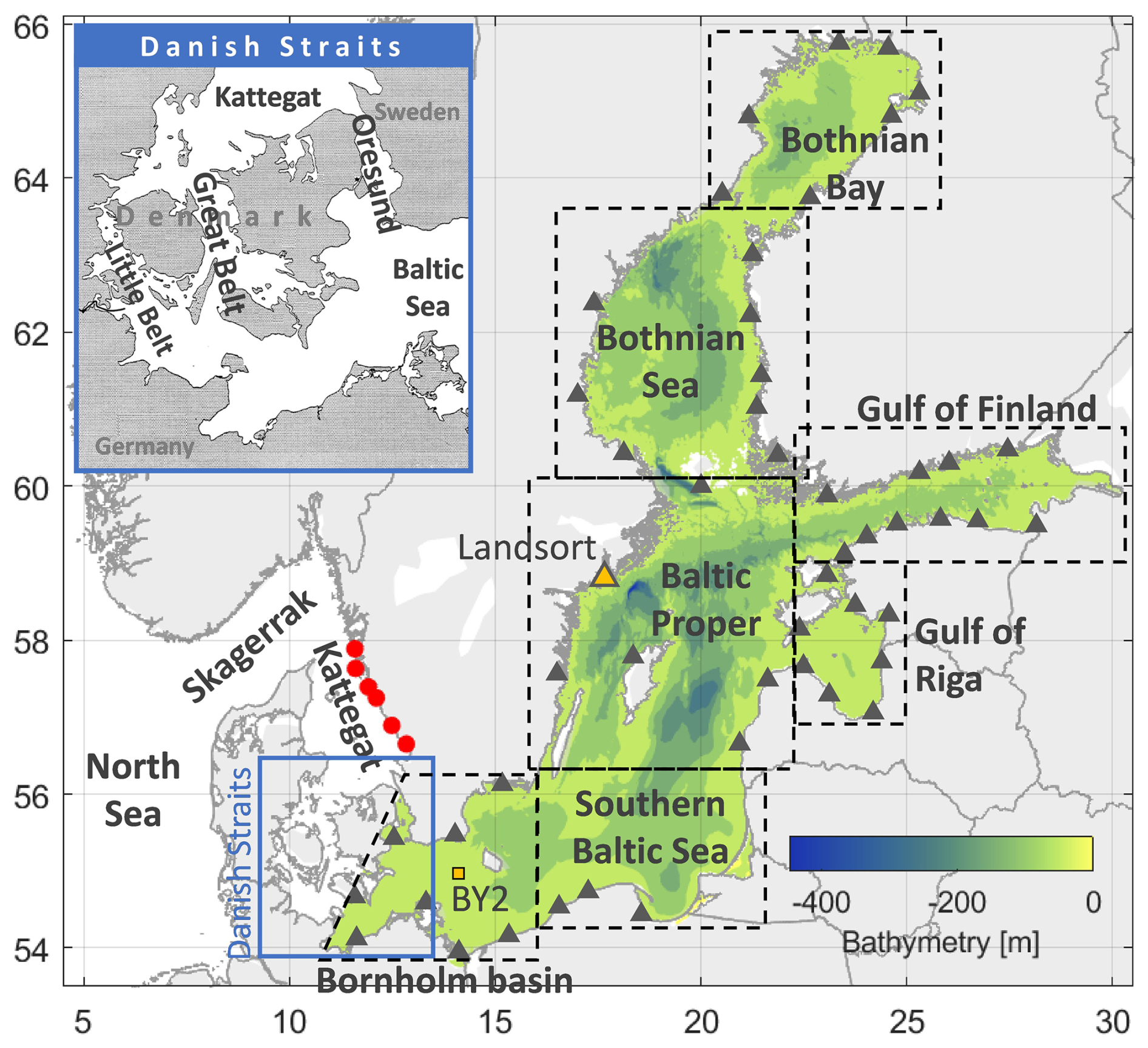
Figure 1 Location of the Baltic Sea and its depth distribution (obtained from GEBCO Compilation Group, 2022). Dashed boxes show the boundaries of the Baltic sub-basins used in this study. Red dots show the location of tide gauges used to calculate volume transport between the Baltic and North Sea. Black triangles denote tide gauge stations that are used for correcting and evaluating the original Nemo-Nordic model in Jahanmard et al. (2023a).

The water structure of the Baltic Sea is highly stratified with a permanent halocline. This stratification results from several factors: (i) voluminous river runoff, with the largest discharges originating from the northern and eastern sections; (ii) restricted and intermittent saline-water inflows from the North Sea through the narrow and shallow Danish Strait; and (iii) limited vertical mixing as processes such as convection, mechanical mixing, entrainment, and advection are known to be limited when tidal amplitudes are relatively small. In addition, a permanent horizontal density gradient exists in the north-to-south direction, making the sea level always higher in the northern regions than in the southern regions (Leppäranta and Myrberg, 2009).

Ideally, the sea level component in hydrodynamic models (HDMs) can be employed for assessing the water budget. However, HDMs are limited by modelling errors and a vertical reference bias that, altogether, constitutes an overall bias which varies both spatially and temporally. This often prevents the link with other sea level data sources (in situ and satellite data). In the Baltic Sea, methods such as interpolation and deep learning were used to examine the bias by employing a common geoid-based vertical reference surface for data sources, through which absolute ocean dynamic topography (DT) was determined (Jahanmard et al., 2022, 2023a). The use of DT enables the calculation of dynamic water volume relative to a physically meaningful reference surface, which is used later in the calculations of the water budget variations and barotropic flows in the following sections.

Regional variations in sea level and coastline dynamics within the Baltic Sea provide a valuable framework for investigating climate variability, extreme events, and processes with global significance, supported by extensive historical and instrumental records (Harff et al., 2017; Weisse et al., 2021). Sea level variability in the Baltic Sea can be categorized into processes that alter the total Baltic water volume and that redistribute water within the Baltic Sea (Samuelsson and Stigebrandt, 1996). Timescales of about half a month or longer predominantly influence changes in the total water volume of the Baltic Sea. Conversely, shorter-term processes, constrained by the limited transport capacity across the Danish Straits, primarily result in the redistribution of water within the basin (Johansson, 2014; Soomere et al., 2015; Weisse et al., 2021). The long-term variability of the Baltic Sea water budget is influenced by basin-averaged mean sea level rise – primarily driven by the influx of mass from the adjacent North Sea as an external signal, with minor contributions from basin-internal water mass redistribution due to local baroclinicity (Gräwe et al., 2019) – and by crustal deformation in the Baltic region caused by postglacial uplift (Richter et al., 2012). The multitude of processes contributing to sea level variations in the Baltic Sea complicates the interpretation of its dynamics and inflows (Weisse et al., 2021). Therefore, quantifying the dynamics of the water column within the Baltic Sea and its interactions with the North Sea and river inflows provides important insights into regional hydrodynamics and water exchange processes.

Utilization of DT allows us to (i) examine the dynamic water volume distribution and its seasonal and sub-basin variations, (ii) quantify barotropic inflow and outflow through the Danish Strait, and (iii) estimate river runoff by using the Baltic Sea water balance computation (Omstedt et al. 2004; Reckermann et al., 2011).

Employing a common geoid-base vertical datum enables us to make modifications to the quadratic friction law used for Baltic water exchange at the Danish Straits (Omstedt, 1987; Mohrholz, 2018) by removing the bias term and considering the water level of the entire Baltic Sea. This, in essence, allows us to calculate all the barotropic water exchanges. To confirm the characteristics of inflows that occur, we also examine in situ bottom salinity data for the Bornholm basin, along with hydrodynamic model data. Previous studies used the difference between Landsort tide gauge station (which roughly represents the Baltic Sea's mean sea level) and the Kattegat sea level. This approach, without considering a common reference surface for sea level determination and relying on a single-point observation, may introduce errors, offsets, or discrepancies. In this study, we show that accurately quantifying DT relative to a geoid-based vertical datum for the entire Baltic Sea (Jahanmard et al., 2023a) enables the determination not only of dynamic volume but also of barotropic Baltic water exchange. Moreover, river runoff can be estimated through water balance calculations.

To understand the study area a bit more, recall that the Baltic Sea is a highly stratified estuary, and, despite the limitation in vertical mixing, water still recirculates by means of the “Baltic Sea haline conveyor belt”, where incoming saline water propagates through the Danish straits (Øresund, Great Belt, Little Belt), upwells within the Baltic, mixes with freshwater inputs, and returns to the North Sea as brackish outflow (Döös et al., 2004). Under favourable wind conditions, major Baltic inflow can occur in the deep water layers of the central Baltic Sea. As a result, both barotropic and baroclinically driven inflows can transport saline water into the halocline or below it, which depends on the density of the inflow water (Reissmann et al., 2009). The inflows of saline water are forced by winds from the west, and outflows are forced by winds from the east.

The winds, when strong enough, can actually reverse the Ekman transport. For example, persistent westerly winds of 2–5 m s⁻¹ can stop the almost constant surface outflow layer of brackish water (Lehmann et al., 2012; Delpeche-Ellmann et al., 2017 and 2021). Also, due to the freshwater surplus, the water volume of the Baltic Sea will increase even though no direct inflow takes place, and this will affect all sub-basins (will be discussed in Fig. 4). As a result, atmospheric forcing plays a major role in the dynamics of the Baltic Sea; it more or less depends on the exact location of the polar front and the strength of the westerlies. Thus, the North Atlantic Oscillation (NAO) index and the Baltic Sea Index can, to some extent, characterize the variations observed in the Baltic Sea (Lehmann et al., 2002; Leppäranta and Myrberg, 2009).

This study aims to use DT of the corrected HDM for the period from 2017 to mid-2021 to quantify (i) the dynamic water volume of the Baltic Sea; (ii) the seasonal and spatial distribution of DT anomalies, which represent internal dynamics and the variation and/or co-oscillation of water volume within the Baltic sub-basins; (iii) barotropic water exchange between the Baltic and North seas; and (iv) total river runoff to the Baltic Sea using the water budget equation. Additionally, examining the seasonal balance of water budget components can reveal biases in existing models. The present paper first introduces the method, with some relevant background concepts, in Sect. 2. The method for assessing the Baltic Sea's dynamics and for computing Baltic inflows is presented in Sect. 3. This is followed by the results and a discussion in Sect. 4 and a conclusion in Sect. 5.

2 Background and dataset

The geoid is the shape of the equipotential ocean surface under the influence of gravity and the rotation of Earth alone. Therefore, its interpretation represents the natural zero vertical datum for sea level (Jahanmard et al., 2021). This implies that any sea level deviation from the geoid (e.g. due to winds, tides, river discharge) is expressed by dynamic topography (DT). Therefore, using a consistent geoid-based vertical datum across diverse sea level data sources allows for the direct integration of model data and observations to determine accurate DT. This data fusion helps mitigate certain modelling and observational errors and addresses absolute sea level variabilities relative to a well-defined reference level (e.g. NAP, Normaal Amsterdams Peil).

Although an equipotential surface is what realistically should be used for expressing physically meaningful heights and depths, in reality, different sea level measurements (e.g. tide gauges, HDMs, and satellite altimetry) may refer to various vertical datums. For instance, tide gauge records are often referenced to national chart datums, which may use the mean sea surface, a geoid-based chart datum, or the lowest astronomical tide as the zero-level surface. Satellite observations provide sea surface height, which is, by definition, referenced to a reference ellipsoid. A geoid model is required to compute DT (Mostafavi et al., 2023). HDMs tend to ideally present sea level with respect to a constant geopotential W as its implicit vertical reference surface (Hughes and Bingham, 2008). Hence, the sea level derived from HDMs is often referred to as DT. However, the vertical reference surface of an HDM may differ from that of the geoid model used for observations in its origin, which can be quantified by a reference bias (Jahanmard et al., 2023a). HDMs may also be subject to modelling errors due to numerical modelling limitations when compared to in situ and satellite altimetry. Therefore, referencing sea level data sources enables the minimization of the modelling errors and provides opportunities for further studies, such as developing data-driven sea level forecasting (Rajabi-Kiasari et al., 2023) and quantifying the components of the Baltic Sea water budget, as will be discussed in this study.

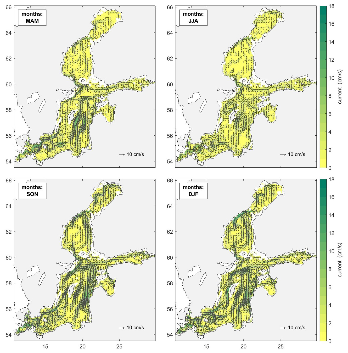
Figure 2 Seasonal surface geostrophic currents computed form the corrected HDM for the period of 2017 to mid-2021.

In this study, we use the Nemo-Nordic model (NEMO NS01) obtained from the Swedish Meteorological and Hydrological Institute (SMHI) and the corrected hydrodynamic model from Jahanmard et al. (2023a). The corrected model was adjusted using a deep learning model to reduce the modelling errors with respect to geoid-referenced tide gauge observations (dataset available in Jahanmard et al., 2023b). The deep learning model resolved the errors (with a range of about 80 cm) through finding relationships between spatiotemporal variables, such as winds and sea level pressure, and modelling errors observed at location of tide gauges.

The assessment of the corrected model demonstrates notable spatial and temporal improvements with respect to satellite observations, with a root mean squared error of 4 cm, limited to less-than-daily errors. In addition, the vertical reference bias between the model and observations was reduced by 18.1 cm, enabling a direct comparison of the corrected DT with observations referenced to the Baltic Sea Chart Datum (BSCD2000) geoid-based vertical datum (Liebsch et al., 2023). The corrected HDM presents an average correlation of 0.98 with 52 tide gauge records, while the original hydrodynamic model shows a correlation of 0.93 (for more details, refer to Jahanmard et al. 2023a). Figure 2 shows the surface geostrophic currents computed from the corrected HDM. This figure confirms that the corrected HDM aligns with the quasi-steady circulation patterns observed in the Baltic Sea (Döös et al., 2004; Soomere and Quak, 2013; Placke et al., 2018; Hinrichsen et al., 2018; Barzandeh et al., 2024). Surface currents in the Baltic Sea are influenced by sea surface tilt; wind stress at the sea surface; and the thermohaline horizontal gradient of density steered by Coriolis acceleration, topography, and friction (Leppäranta and Myrberg, 2009; Soomere et al., 2011). As a result, this figure indicates that our DT correction approach not only improves the accuracy of sea surface determination by integrating model data and observations but also preserves the underlying circulation patterns.

Water transport between the Baltic and the North Sea can be assessed by comparing the volume of water stored in the Baltic basin with the water column in the Kattegat basin (discussed in Sect. 3.1). For this purpose, the dynamic topography of the Kattegat basin (DT_K) is determined by averaging six geoid-referenced tide gauge readings located in Kattegat (Fig. 1). Tide gauge records are referenced to the same vertical datum, BSCD2000, as the corrected HDM. Therefore, the difference in DT between the two basins reflects deviations from the equipotential surface.

To investigate the occurrence of barotropic Baltic inflow events (discussed in Sect. 3.2) with salinity changes in the southern sub-basins, the bottom salinity dataset is obtained from the Baltic Sea Physics Reanalysis model (Baltic Sea Physics Reanalysis, 2024). We evaluated this dataset with CTD (conductivity, temperature, and depth) observations at station BY2, located in the Bornholm basin, which shows a good agreement between the model and observations. The bottom salinity signal is averaged over the southern Baltic sub-basins indicated in Fig. 1. Comparing changes in the spatial average of bottom salinity in the sub-basins can indicate events of saline-water inflow into the Baltic Sea.

We also obtained the European Hydrological Predictions for the Environment (E-HYPE) dataset (Berg et al., 2021) for the period of this study to compare with the river inflow computed from the Baltic water volume balance. The Nemo-Nordic model is also forced by E-HYPE river discharge (Kärnä et al., 2021). The river discharge signal from the E-HYPE model is determined by integrating the river discharges along the boundary of the Baltic Sea on a daily timescale.

3 Method

3.1 Dynamic water volume

The Baltic Sea has an average volume of 21 205 km³, with an annual addition of about 480 km³, mainly from river runoff and net atmospheric flux (precipitation minus evaporation). The volume decreases via outflows through the Danish Straits. The total freshwater budget remains consistently positive due to substantial river runoff, with monthly runoff ranging from 0.85 to 2.16 km³ d⁻¹ (Leppäranta and Myrberg, 2009).

Conventionally, the water volume is computed by integrating the water column from the seafloor to the sea surface. To study the water balance of a basin, it is beneficial to separate the total water volume into two components: the dynamic water volume V(t), which fluctuates over time, and the constant water volume V₀. These two components can be distinguished using an equipotential surface (e.g. a geoid model). Therefore, considering DT to be a sea level variation relative to a stable geoid-based vertical reference surface, the dynamic volume is calculated through the spatial integration of DT fluctuations. Hence, the constant water volume is the integration of water columns from the seafloor to the geoid surface.

In fact, V(t) represents the volume variations from V₀ due to factors such as inflow or outflow, river runoff, and net atmospheric flux. Note that the constant volume can also experience changes over the years due to sediment redistribution and/or vertical land movements (e.g. glacial isostatic adjustment). However, its dynamic effects on the basin are reflected in the dynamic component as the geoid surface is (quasi-)static. The slow changes in the geoid over time due to factors such as glacial isostatic adjustment and variations in the Earth's mass distribution can be accounted for in the computations (Kakkuri and Poutanen, 1997). Therefore, total water volume V(t) is determined as follows:

$$\begin{array}{}\text{(1)}& \begin{array}{rl}V\left(t\right)& =V_{\mathrm{0}}+V\left(t\right)=\underset{A}{\iint }H(x,y)\mathrm{d}x\mathrm{d}y\\ & +\underset{A}{\iint }\text{DT}(x,y,t)\mathrm{d}x\mathrm{d}y,\end{array}\end{array}$$

where H represents the charted depth relative to the geoid surface, and x and y represent the Cartesian zonal and meridional coordinates, respectively. In this study, the focus is on the utilization of dynamic water volume V(t).

To examine the variation in the dynamic water volume for each sub-basin, their volume was normalized by the sub-basin area A_b. This term is equivalent to the spatial mean of DT for each sub-basin (DT_b), with the distinction that meridian convergence is also considered. Therefore,

$$\begin{array}{}\text{(2)}& {\text{DT}}_{\mathrm{b}}\left(t\right)={\displaystyle \frac{\mathrm{1}}{A_{\mathrm{b}}}}{V}_{\mathrm{b}}\left(t\right),\end{array}$$

where V_b(t) is the dynamic water volume obtained from Eq. (1) for sub-basin b. DT_b enables the determination of the water balance between sub-basins, as will be discussed in Sect. 4.1.

Therefore, one can compute the spatial anomaly of DT_b by subtracting the spatial mean DT of the entire Baltic Sea. The variable DT anomaly (DTa) represents relative variations in DT among the sub-basins. This can indicate co-oscillations between sub-basins and enable the assessment of the correlation between DT distribution in the Baltic Sea and factors such as wind. Therefore,

$$\begin{array}{}\text{(3)}& {\text{DTa}}_{\mathrm{b}}\left(t\right)={\text{DT}}_{\mathrm{b}}\left(t\right)-{\text{DT}}_{\text{BS}}\left(t\right),\end{array}$$

where DT_BS represents the spatial mean DT (according to Eq. 2) over the entire Baltic Sea. The variable of DTa_b can, in fact, serve to illustrate the internal dynamics of the Baltic Sea and reveals the co-oscillations among its sub-basins.

3.2 Water exchange between the Baltic Sea and the North Sea

The saline-water exchange between the Baltic Sea and the North Sea typically occurs somewhere between the Kattegat and the Danish Straits, which varies depending on the prevailing baroclinic and barotropic forcing conditions. This study examines the barotropic water exchange between the Baltic and North seas, where the Baltic Sea maintains equilibrium with the open ocean through the shallow, narrow Danish Straits (Omstedt et al., 2014). These straits act as a low-pass filter for the Baltic Sea, preventing the entry of high-frequency variations from the Nordic Sea (Weisse and Hünicke, 2019). Water exchange is driven by differences in sea level (barotropic) and density gradients (baroclinic) between the Kattegat and Arkona basin. Baroclinic events, primarily driven by salinity gradients, occur mainly during calm summer conditions. For most of the year, barotropic forcing exceeds baroclinic forcing considerably as wind forcing (especially zonal) and air pressure establish sea level differences between the Kattegat and Baltic Sea (Mohrholz, 2018; Leppäranta and Myrberg, 2009).

Due to the anisotropic wind properties of the Baltic Sea (Soomere, 2003) and the requirement of favourable conditions that allow water exchange between the Baltic and North Sea (Zhurbas and Väli, 2022), these input–output events typically occur intermittently on different scales (small, medium, or large). Also, inflows have a seasonal trend, with intense events usually occurring in November–January and with a minimum in May. Inter-annual and intra-annual variations also occur and are influenced by air pressure, winds, and sea level differences between the Baltic and North Sea.

However, replenishing the deep bottom waters of the Baltic Sea requires a large inflow, often referred to as a major Baltic inflow (MBI). Such MBIs typically occur once per decade, and, apart from increasing the total water volume in the Baltic Sea, they also bring salty, oxygen-rich waters and dense water to the deep areas of the Baltic, extending as far as the Gotland basin (Purkiani et al., 2024). There was no MBI during the period of this study; therefore, our focus is not on determining MBI, for which several methods have been employed (Matthäus, 1993; Lehmann and Post, 2015). Instead, we demonstrate how the corrected HDM model can be used to quantify all the barotropic water exchanges between the Baltic Sea and North Sea basins. Utilizing DT with a common reference surface facilitates accurate calculation of sea level slopes between the two basins.

Quantifying volume transport through the Danish straits requires consistent time series of the mean sea levels of the Baltic Sea and Kattegat, along with river runoff data (Mattsson, 1996; Mohrholz, 2018). In Mohrholz (2018), the mean sea level time series for the Baltic was derived from tide gauge measurements at Landsort, which is a reasonable representation of the mean sea level of the Baltic. This study employs a similar approach with some modifications. The main difference is the use of the mean DT of the entire Baltic Sea from the corrected model and the concept of using a stable geoid-based reference surface, which allows for an accurate determination of dynamic water volume and DT inclination between the Baltic Sea and Kattegat basin, thus making the quantification simpler and more accurate. As a result, the barotropic flow through the Danish Straits can be quantified by the quadratic frictional law:

$$\begin{array}{}\text{(4)}& Q\left(t\right)=\sqrt{{\displaystyle \frac{{\text{DT}}_{\text{BS}}\left(t\right)-{\text{DT}}_{\text{K}}\left(t\right)}{K_{\mathrm{f}}}}},\end{array}$$

where Q represents the flow rate, and positive values indicate outflow from the Baltic Sea. DT_BS and DT_K are, respectively, the DT of the Baltic Sea and of the Kattegat, and K_f is the empirical flow resistance coefficient (Stigebrandt, 1983). In this equation, offset correction is no longer needed as both DT measurements were taken based on a common reference surface. The value of K_f is 2.03 × 10⁻¹⁰ s² m⁻⁵, with an uncertainty of approximately 10 % (Mattsson, 1995, 1996).

3.3 Water budget of the Baltic Sea

The water budget of the Baltic Sea consists of several main parameters, such as river runoff R, evaporation E, precipitation P, and inflow and outflow through the Danish Straits Q (see Eq. 5). The two main parameters are Baltic inflows and outflows and mean river discharge. The mean annual river discharge of 436 km³ is almost as dominant as the total inflow of saline water from the North Sea. The net atmospheric flux (precipitation and evaporation) is about 10 times smaller than the river inflow, and it shows positive values from January to August and negative values from September to December (Leppäranta and Myrberg, 2009). As a result, the total freshwater budget of the Baltic Sea, primarily dominated by river inflow, consistently remains positive on a monthly timescale. The following simplified equilibrium equation can express the conservation of Baltic water mass and account for temporal variations in water volume (Omstedt et al., 2004; Reckermann et al., 2011; Mohrholz, 2018):

$$\begin{array}{}\text{(5)}& {\displaystyle \frac{\mathrm{d}V\left(t\right)}{\mathrm{d}t}}=R\left(t\right)+\left(P\right(t)+E(t\left)\right)-Q\left(t\right),\end{array}$$

where R, P, E, and Q are the rates of river runoff, precipitation, evaporation, and Baltic flow, respectively. Given the fact that the water volume time series V(t) was derived from Eq. (2) and the Baltic flow rate Q(t) was determined by Eq. (4), the rate of total river runoff can also be derived from an accurate DT of the Baltic Sea as follows:

$$\begin{array}{}\text{(6)}& R\left(t\right)={\displaystyle \frac{\mathrm{d}V\left(t\right)}{\mathrm{d}t}}-\left(P\right(t)+E(t\left)\right)+Q\left(t\right).\end{array}$$

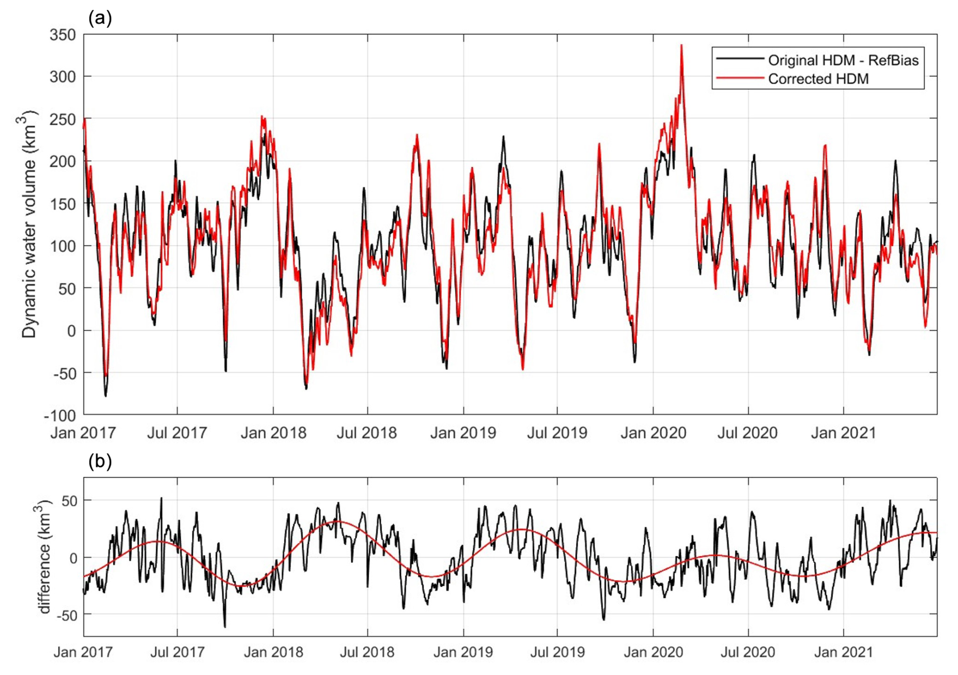
Figure 3 Dynamic water volume V(t) of the Baltic Sea during the designated period. Panel (a) shows the water volume from the Nemo-Nordic model (black) and the corrected model (red). Panel (b) presents the discrepancy between the two models (original – corrected) in black, whereas its smoothed version is in red.

The net atmospheric flux (P+E) is the sum of the precipitation and evaporation, where the positive evaporation is downward. The precipitation and evaporation datasets were downloaded from ERA5 hourly data (Hersbach et al., 2023). The precipitation parameter is the accumulated rain and snow over the Baltic Sea. The precipitation and ice melting on land, as well as groundwater flow, are included in the total river runoff. It should be emphasized that the steric correction is incorporated into the corrected HDM, whereby, as a result, the density-related volume changes are included in the term $\mathrm{d}V/\mathrm{d}t$. In addition, the volume change due to land uplift was accounted for through the definition of using absolute DT relative to a reference epoch. Comparing Baltic inflows and outflows and total river runoff, computed from the original and corrected Nemo-Nordic models, can also provide insights into the source of seasonal bias in sea level modelling (see Sect. 4.1), as will be shown in the “Results and discussion” section.

4 Results and discussion

By using the corrected DT, a more accurate quantification and examination of the Baltic sea dynamics and water budget components can be achieved. Such a method, to our knowledge (Sect. 3), has not been utilized before. In this section, we present (i) the visualization and examination of the Baltic Sea's dynamic water volume and its internal dynamics through the DT anomalies in different sub-basins of the Baltic Sea, (ii) quantification of all barotropic exchanges between the Baltic Sea and North Sea, (iii) utilization of the water budget equation to derive river runoff, and (vi) examination of the seasonal distribution of the dynamic water volume.

4.1 Dynamic water volume and co-oscillation of sub-basins

The dynamic water volume of the Baltic Sea is governed by several factors functioning on different timescales, with both periodical and irregular frequencies. The sub-basins also oscillate under the influence of atmospheric forcing and permanent features, such as geometry, bathymetry, and their location. In this section, we present the changes in water volume within the Baltic basin and the internal redistribution of water columns between sub-basins using DT anomalies (Eq. 4), which represent a normalized change in sub-basin water volume.

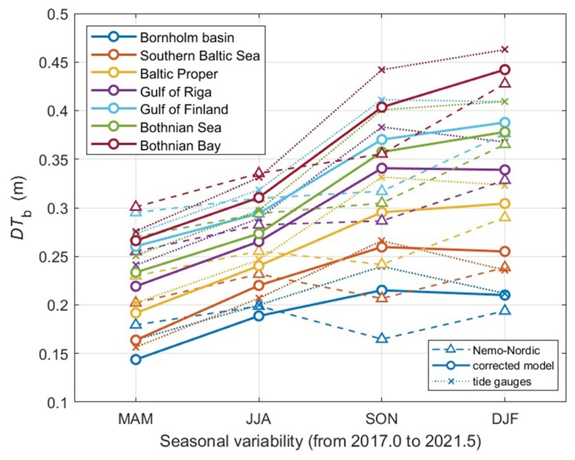
Figure 4 Seasonal DT_b computed from Eq. (2) for the Baltic sub-basins, represented by different colours. Dashed, solid, and dotted lines denote DT values from the original Nemo-Nordic model, the corrected model, and tide gauge observations, respectively.

Figure 3 shows the dynamic water volume of the Baltic basin, computed using both the corrected and the original HDM. The difference between the two (shown in the bottom panel) demonstrates the impact of modelling errors on representing the dynamics of the Baltic Sea. To align origin zero levels between the original Nemo-Nordic model and the corrected model, the constant reference bias (18.1 cm) was removed from the original model (see Jahanmard et al., 2023a, for details). Figure 3 shows that the dynamic water volume of the Baltic Sea varies from −75 to 340 km³, and the difference between the two models reveals a seasonal error in water volume estimation by the Nemo-Nordic model, ranging from −60 to 50 km³.

The original Nemo-Nordic model tends to overestimate water volume during spring and summer and underestimate it during autumn and winter months. A change of 10 km³ in water volume is associated with an approximate sea level variation of 2.6 cm based on the geometry of the study area. It would be worth noting that the steric effect correction was also included in the corrected DT (Jahanmard et al., 2023a), which may contribute to the seasonal difference.

Other drivers also contribute to the overestimation or underestimation of the original Nemo-Nordic model. For instance, peak river discharge in the Baltic Sea, primarily driven by atmospheric precipitation and snowmelt, occurs between April and June (Graham, 2004; Raudsepp et al., 2023). This may have introduced a seasonal bias into the model. Additionally, the discrepancy could be related to underestimating wind forces, as southwesterly and westerly winds dominate in autumn and winter, usually resulting in sea level accumulation in the eastern and northern regions of the Baltic Sea (Alenius et al., 1998). Further investigation is needed to confirm these hypotheses.

Figure 4 shows the seasonal variation of DT_b, the spatial average of sub-basins, for both the corrected and the original HDM, along with the average tide gauge readings from the sub-basins. Key findings include the following: (i) the corrected DT closely follows the seasonal pattern observed by tide gauges, (ii) sub-basin DT is higher in autumn and winter, and (iii) water levels in the northern sub-basins (Bothnia Bay, Bothnia Sea, and Gulf of Finland) are consistently higher than in the southern sub-basins (Bornholm basin and southern Baltic Sea). This is mainly due to permanent horizontal water density differences, driven primarily by salinity, which result in a higher sea level in the north. On average, sea level is expected to decline by 35 to 40 cm from the Bay of Bothnia to the Skagerrak (Leppäranta and Myrberg, 2009), which is partially reflected in Fig. 4, where the difference between Bothnia Bay and Bornholm basin is 24 cm in winter and 13 cm in spring. Additionally, the original Nemo-Nordic model displays different seasonal variations compared to the tide gauges and the corrected model, with its discrepancy remaining relatively constant across sub-basins. The difference between the tide gauge and the corrected model arises because the corrected model averages DT across the entire sub-basin, whereas tide gauges reflect DT variation at specific locations. These two measures align when the corrected model is averaged at the tide gauge locations.

Table 1 Annual and seasonal average dynamic topography (in metres) for sub-basins. Numbers in parentheses indicate the difference between seasonal and annual means. The sub-basins are listed from south to north (see Fig. 1).

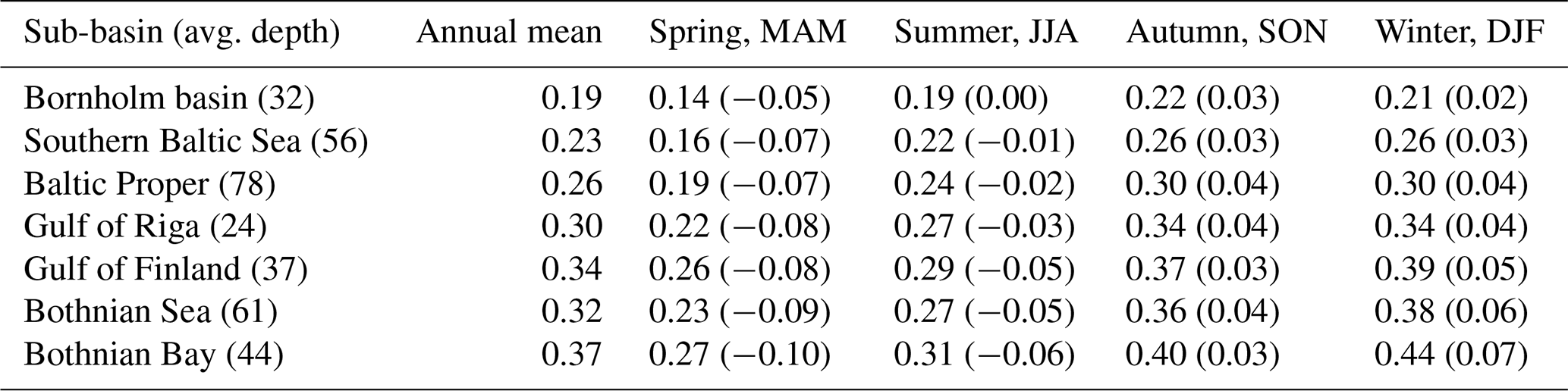
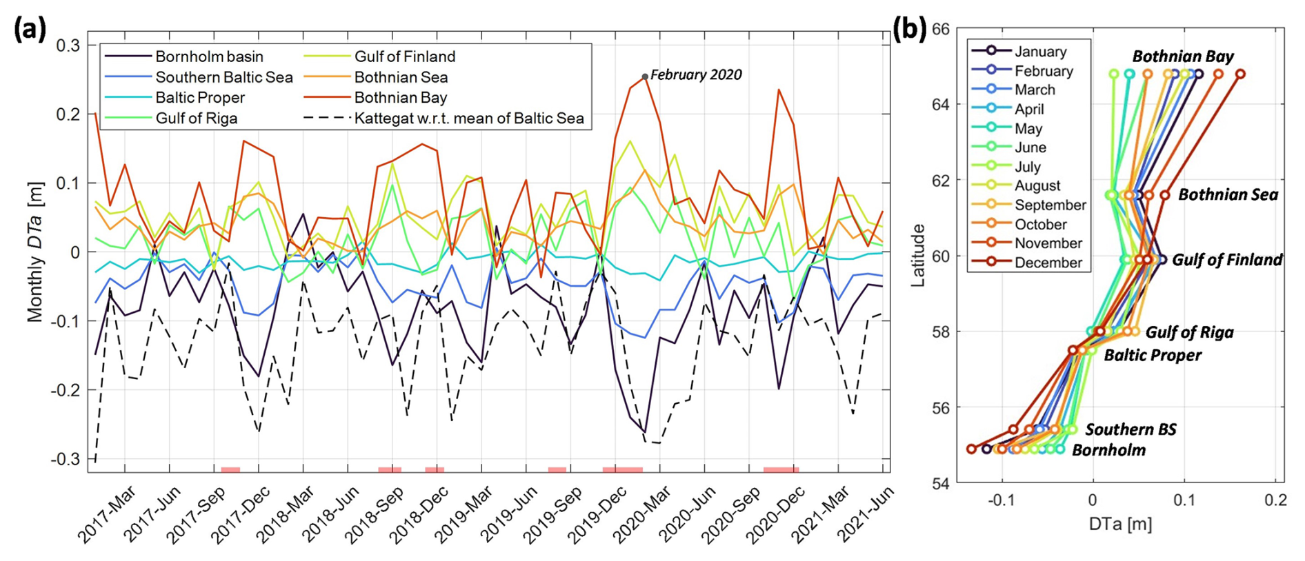
Figure 5 Spatial anomalies in DT of sub-basins. (a) Monthly mean of DTa for different sub-basins, along with mean DT of Kattegat with respect to the mean of the Baltic Sea. (b) Climatological monthly mean DTa for the designated time period plotted against the latitude midpoint of sub-basins.

The Baltic Sea water level increases in autumn (SON) and winter (DJF) and decreases in spring (MAM) and summer (JJA). This seasonal increase in autumn and winter months is attributed to the following: (i) dominant southwesterly and westerly winds pile up water in the eastern and northern sub-basins; (ii) river inflow is still significant, and the freshwater budget remains positive (Leppäranta and Myrberg, 2009); and (iii) Baltic inflow shows the trend of being highest for these months. Table 1 presents the mean DT of the Baltic sub-basins, as well as their seasonal and annual distributions obtained by applying Eq. (3).

Anomalies in DT (DTa from Eq. 3) allow for the analysis of oscillations amongst sub-basins at different timescales. This is done by subtracting the spatial mean DT of the entire Baltic Sea from the DT of any given sub-basin at an identified timescale. As a result, DTa(t) represents the water level of sub-basins in relation to each other. Figure 5 illustrates the monthly DTa of the sub-basins shown in Fig. 1. We observe a consistently positive DT in the northern and eastern sub-basins and negative values in the southern region of the Baltic Sea, along with co-oscillation between sub-basins on a monthly timescale. To emphasize the greatest difference observed between basins, we highlight an extreme case that occurred in February 2020, where the difference between the DT in the northern and southern parts of the Baltic Sea reached up to 50 cm. Figure 5b shows the seasonal perspective, where an obvious increase in sea surface tilt during autumn and winter months occurs, with a maximum difference of 32 cm between the northern and southern basins in December. The occurrence of these maximum differences usually takes place during the autumn and winter months, when predominant southwesterly and westerly winds are the strongest (Leppäranta and Myrberg, 2009). Contrarily, the sea surface shows minimal DTa inclination in summer months. In general, the Bornholm and Bothnian Bay basins experience the highest variability throughout the year (32 and 29 cm, respectively), while the Baltic Proper shows the least variation.

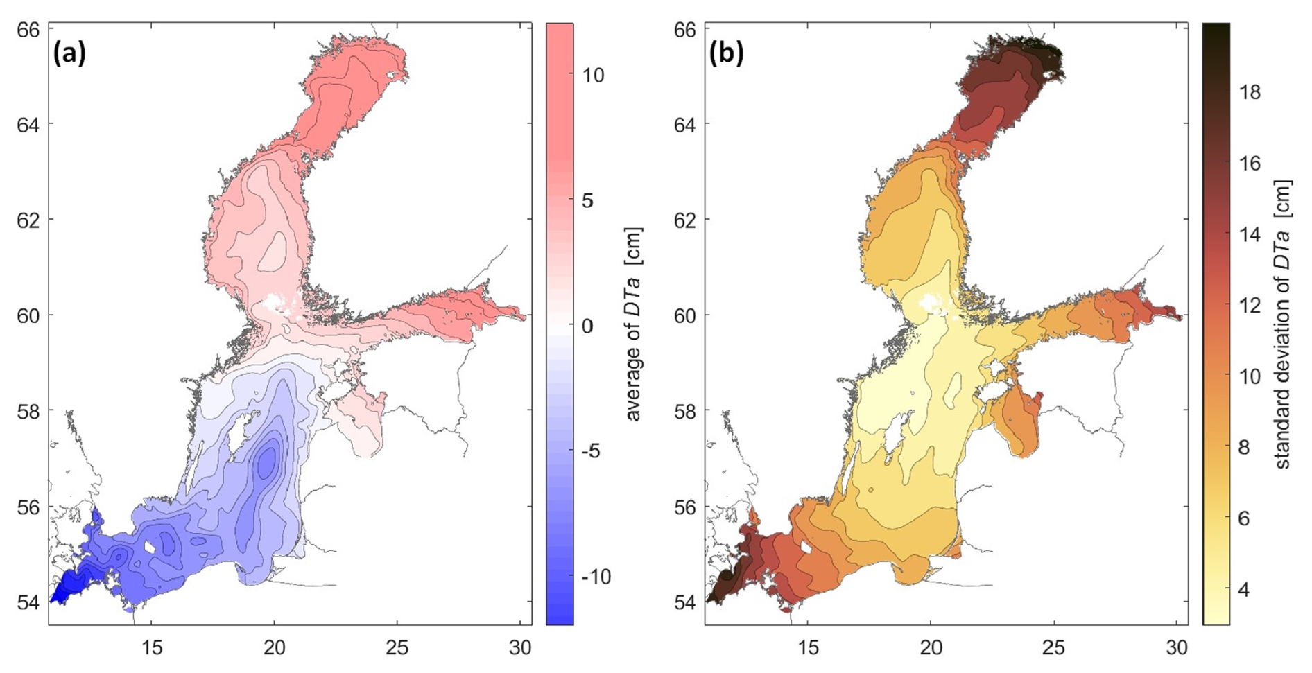
Figure 6 Temporal mean (a) and standard deviation (b) of DTa (Eq. 3), computed at model grid points based on hourly data.

The Kattegat and Danish Straits are known as transition areas that allow the exchange of the salty North Sea waters and the fresher Baltic Sea waters. The variation in the DT of Kattegat relative to the mean of the Baltic Sea is also depicted in Fig. 5a by a dashed line. We observe that this variation consistently remains below the average water level of the Baltic Sea. This positive sea level compared to the Kattegat leads to a predominant outflow from the Baltic Sea. However, during some events on this monthly timescale, the DTa of Kattegat surpasses that of the southern sub-basins. This consequently causes the inflow of saltwater into the southern Baltic basin (highlighted in Fig. 5a by red boxes). These results of the exchange of the Baltic and North Sea waters are examined more deeply in Sect. 4.2.

Figure 6 shows the average DTa and its standard deviation at model grid points as computed from hourly data. On average, the northern and eastern sections of the Baltic Sea display a consistently positive dynamic topography of about 10 cm relative to the mean states of the Baltic Sea, while the southern part exhibits lower DTa (about −10 cm) than the Baltic average. The variability in DTa across the Baltic Sea (Fig. 6b) can highlight the first barotropic basin mode (Wubber and Krauss, 1979) under the influence of atmospheric forcing. High-frequency DT variations in the Baltic Sea are internally isolated due to the characteristics of the Danish Straits (Weisse and Hünicke, 2019), which result in the Baltic seiches (Jönsson et al., 2008). The variability in DTa increases to over 15 cm with distance from the Baltic Proper. Greater DTa variability may indicate areas with a higher potential to be impacted by extreme sea level events. Areas with a high standard deviation and average DTa overlap with some of the identified areas of coastal erosion, especially those in the Gulf of Finland, the Gulf of Riga, and the southern Baltic Sea (Weisse et al., 2021; Pindsoo and Soomere, 2020).

As observed in Fig. 6 for the northern Baltic Proper, the DTa values approach 0 cm, and the standard deviation is less than 4 cm. This is also complemented by Fig. 5b, which shows that the seasonal variation in the Baltic Proper is very small compared to in other sub-basins. These observations signify that this particular region in the Baltic Proper can be used to closely represent an equilibrium mean DT for the entire Baltic Sea. This indicates that any significant changes in DT values in this area may be used as climatic change indicators or for the occurrence of the ocean dynamics of the Baltic Sea (BS) (e.g. Baltic inflows).

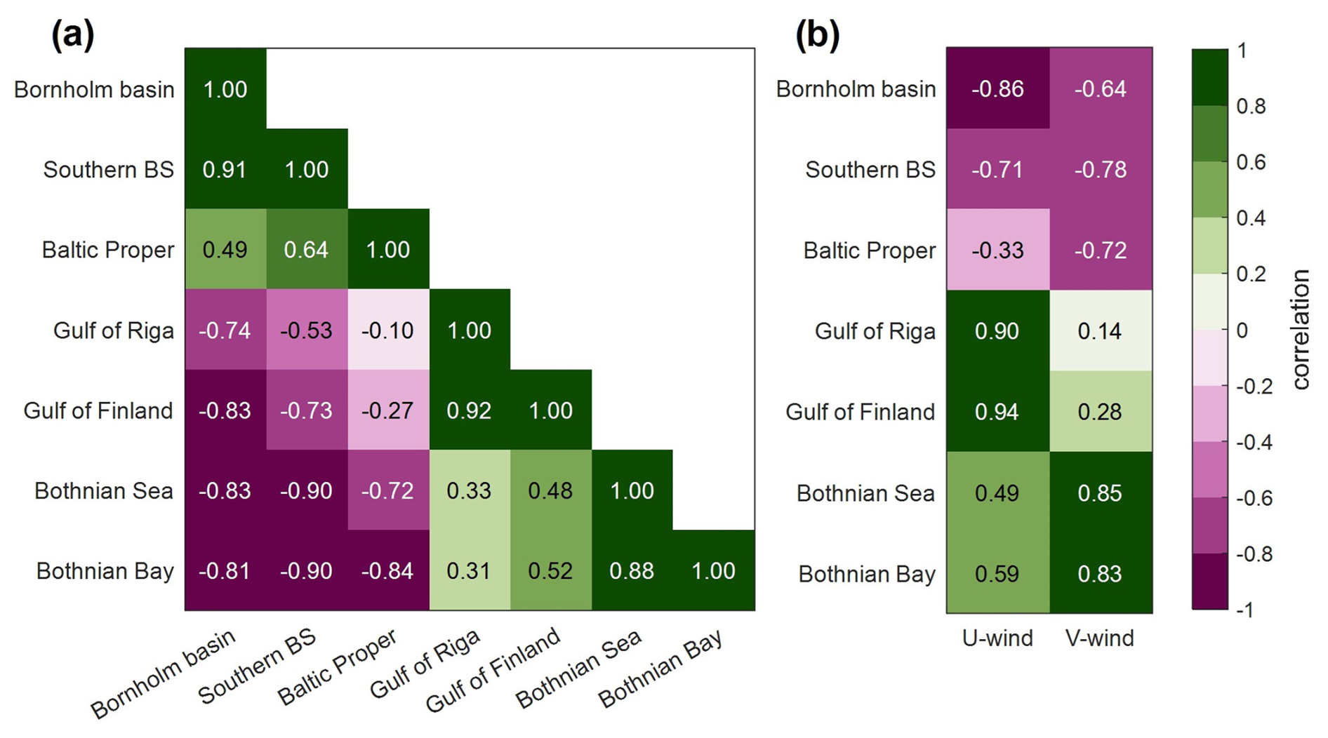
Figure 7 Correlation of sub-basin DTa on a monthly timescale (a) and the correlation of DTa with the predominant wind across the Baltic Sea.

The co-oscillation amongst sub-basins is determined by the correlation coefficient of DTa on a monthly timescale. Figure 7 shows a strong anti-correlation between the southern and northern (eastern) sub-basins of about −0.90 (−0.80). Since the DTa of sub-basins was normalized to the mean sea level of the Baltic Sea, the oscillation of DTa is mostly controlled by atmospheric forcing across the entire basin. Figure 7b shows the correlation between sub-basin DTa and the predominant wind over the Baltic Sea. The northern (eastern) regions display a strong correlation of 0.85 with meridional winds (0.94 with zonal winds). This can indicate that the highest DTa variation and the monthly dynamics of these sub-basins are mostly driven by winds, especially westerly and southwesterly winds, which pile up water in the northern and eastern sub-basins. Also, strong anti-correlations between the DTa values of southern basins and winds are observed.

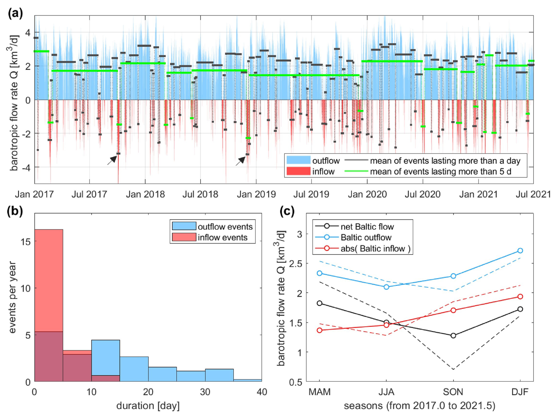
Figure 8 Barotropic Baltic water exchange calculated from hourly time series of dynamic topography inclinations between the Baltic Sea and the Kattegat basin. (a) Time series showing positive (outflow, in blue) and negative (inflow, in red) Baltic flow rates, along with the mean values of events lasting more than 1 and 5 d. (b) Histogram of event duration per year for events longer than 1 d. (c) Average flow rates over seasonal timescales, with solid lines for the corrected model and dashed lines for the original model.

4.2 Barotropic water exchange between the Baltic Sea and the North Sea

As was described in Sect. 3.2, the DT inclinations between the Kattegat and the Baltic sea can be used to indicate the occurrences of barotropic water exchanges (inflow and outflow) between the Baltic Sea and the North Sea. This can be accomplished by computing the flow rate (Q) based on Eq. (4). Thus, the computed barotropic Baltic flow rate through the Danish Straits for the period of 2017 to mid-2021 is presented in Fig. 8. Note that, for the period examined in this study, no MBI occurred; thus, the results described below relate to medium and small exchanges.

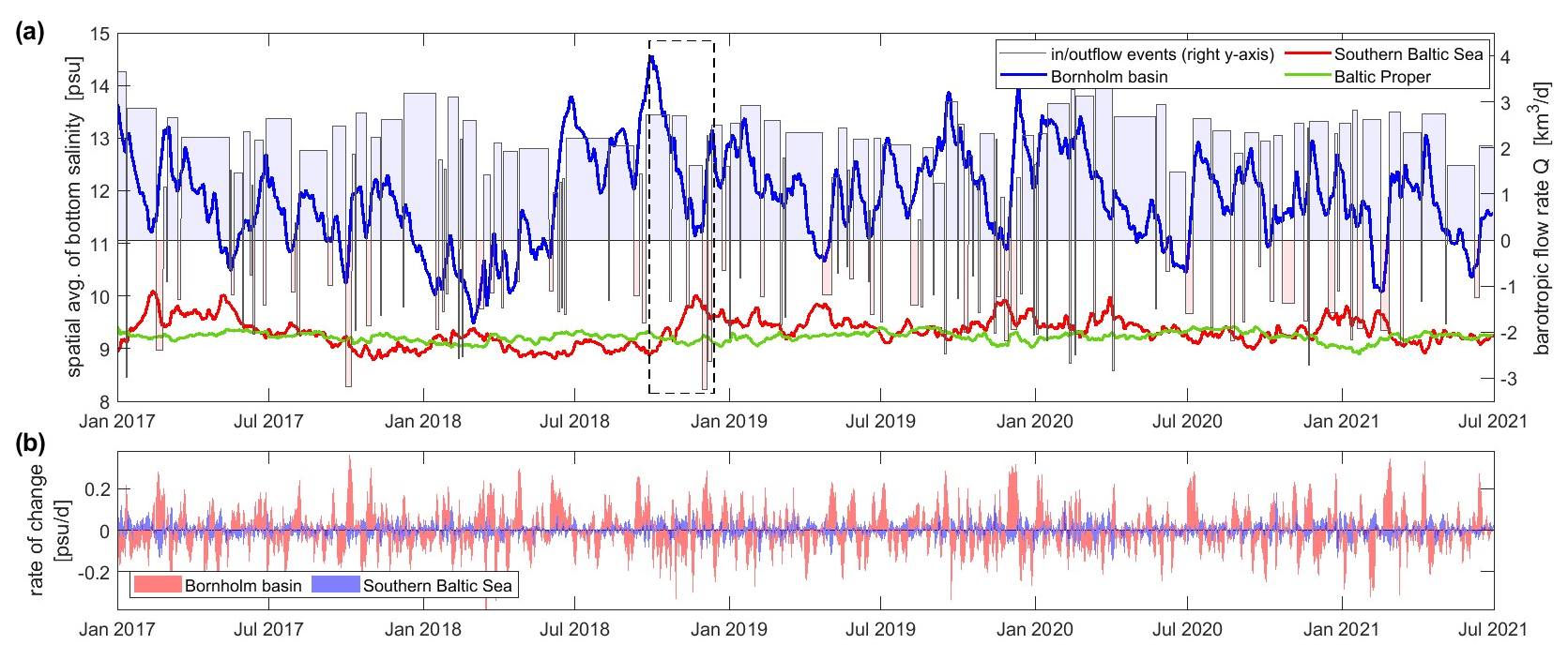
Figure 9 Bottom salinity: (a) spatial average of bottom salinity in southern basins, along with barotropic flow rate from Fig. 8a on the right y axis. (c) Rate of change in (time-derivative) bottom salinity.

At first glance, the average outflow and inflow rates display high-frequency signals (Fig. 8a). However, by applying specific temporal criteria to filter out the high-frequency variations, it becomes possible to distinguish the relevant inflow and outflow events. For the statistical analysis, the inflow events (when negative) and outflow events (when positive) can be distinguished using the criterion outlined in Fischer and Matthäus (1996), where each event should last at least a day (as indicated by the horizontal black lines in Fig. 8a). Therefore, the histogram of event durations (Fig. 8b) presents the number of inflow and outflow events based on their duration. In Fig. 8a, another criterion for classifying each event that lasts at least 5 d is also indicated by the green lines.

Figure 8b shows that most inflow events, based on the 1 d lasting criterion, have a duration of less than 5 d, with about 16 events occurring per year. For inflow duration of more than 5 d, the number of occurrences is about four events per year and less than one event per year for durations lasting more than 10 d. However, this result is sensitive to changes in event classification criteria, which subsequently alter the event histogram. Nevertheless, the overall inflow pattern confirms that Baltic Sea inflow events are sparse and brief compared to the outflow.

Two inflow events that were significant in terms of duration and magnitude occurred in October 2017 and November 2018 (denoted by arrows in Fig. 8a). Each event lasted about a week, with inflow rates of 3.19 and 3.24 km³ d⁻¹, respectively. The total volume of inflow water for the events was approximately 22.5 km³, which is small compared to MBIs (e.g. 198 km³ in December 2023 for 14 d; Purkiani et al., 2024) but comparable to the average daily outflow (2.36 km³). Recall that, due to the predominantly positive freshwater budget dominated by river runoff, the Baltic Sea consistently experiences outflow. These outflows occur at different rates, with a seasonal pattern (Leppäranta and Myrberg, 2009).

Figure 8c shows the seasonal mean values of the calculated Baltic flow rate, with an average outflow of 2.36 km³ d⁻¹ and average inflow of 1.6 km³ d⁻¹. These values are closely aligned with the long-term mean water exchanges reported by Liljebladh and Stigebrandt (1996), which are 2.59 km³ d⁻¹ for outflow and 1.3 km³ d⁻¹ for inflow. In winter, both inflow and outflow rates reach their maximum value due to increased wind variations and storm conditions. Concerning the net Baltic flow, a consistent positive outflow is observed on a seasonal timescale, with a maximum in spring and a minimum in autumn. Interestingly, the dashed black line in Fig. 8c represents the net Baltic flow from the original Nemo-Nordic model, which indicates a significant difference in autumn.

To assess the occurrence of barotropic inflow events with salinity changes in the southern sub-basins, we compare the bottom salinity signals of the sub-basins with the Baltic flow rate in Fig. 9a. The barotropic flow lasting more than 1 d (from Fig. 8a) is shown in the background (right y-axis). The bottom salinity of the Bornholm basin and the southern Baltic Sea follows a pattern: it increases with sustained inflow and decreases when there is no significant inflow. This observation in the southern Baltic Sea basin suggests that the medium and small inflow events can reach as far as the southern basins (red line) but are not effective enough to introduce saline water into the deeper waters of the Baltic Proper.

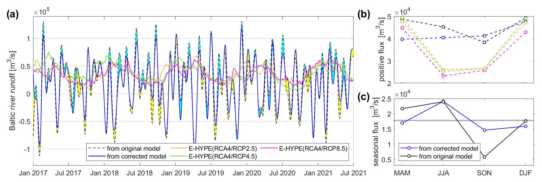
Figure 10 River runoff computed from Eq. (6) using both original and corrected model: (a) daily timescale, along with total river discharge obtained from E-HYPE dataset; (b) seasonal averages of positive runoff (flux into the sea) and E-HYPE river discharge; (c) seasonal average of the river runoff computed from original and corrected model.

A pattern observed is that, prior to certain inflow events, such as the one that occurred in October–November 2018, highlighted by the dashed box, the two southern sub-basins mix in such a way that the bottom salinity decreases in the Bornholm basin while increasing in the southern Baltic Sea basin. The rates of bottom salinity change for these two sub-basins are also presented in Fig. 9b. This figure shows positive spikes in the Bornholm sub-basin when the 1 d lasting criterion denotes an inflowing event. This pattern, where bottom salinity in these sub-basins starts to mix before an inflow event, may be influenced by factors such as wind and pre-event mixing. Further research can explore this topic.

4.3 River runoff

The voluminous river runoff from the Baltic Sea catchment areas is a significant contributor to the water budget of the Baltic Sea. In this section, the total river runoff is indirectly retrieved using Eq. (6) by considering the conservation of Baltic Sea water mass. Note that the computed river runoff also includes groundwater flow into the Baltic basin as we simplified this equation (cf. Eq. 6 of this paper and Eq. 1 in Omstedt et al., 2004).

Figure 10a shows the runoff computed from the original and corrected model. A fourth-order Butterworth low-pass filter with a cutoff frequency at $\mathrm{1}/\mathrm{30}$ d⁻¹ was applied to remove undesirable high-frequency components of the runoff. The river runoff derived from the corrected model (blue line) varies in a range from −1 × 10⁵ to 1.2 × 10⁵ m³ s⁻¹. Positive runoff indicates the addition of flow to seawater, whereas negative runoff signifies the withdrawal of water from the sea. This withdrawal may result in temporary inflows of seawater into the river or estuarine system due to rising Baltic water level or storm surges. In this figure, the yellow area indicates the period during which the river runoff of the corrected model was computed to be higher than that of the original model, while the light-blue area indicates the opposite.

The river discharge signal from three versions of the E-HYPE model is also shown in Fig. 10a and b. Note that the Baltic river runoff estimated from the water balance calculation can differ from the river forcing used for the model as these are two different concepts for deriving river discharge. Based on our knowledge, the E-HYPE model does not specifically account for seawater withdrawal (i.e. reverse flow from sea to land). It is typically used to model the flow from land to sea as the model considers the sea basin as the downstream. In comparison with the computed runoff using Eq. (6), it can be observed that the presented approach is able to determine the flow interactions between land and sea in more temporal detail due to the accurate water balance computation. This estimation can potentially be coupled with a hydrological model.

Table 2 Seasonal variation in the Baltic dynamic water volume and water budget components.

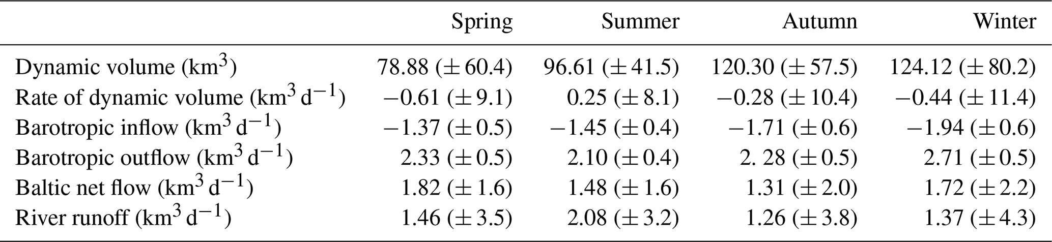
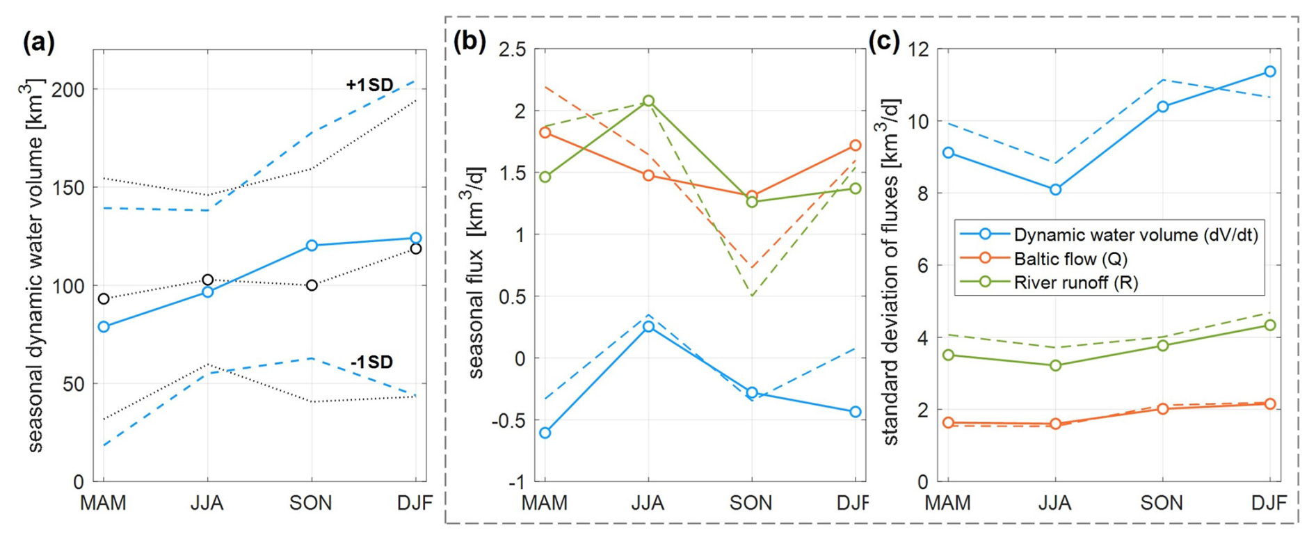
Figure 11 Seasonal variability of dynamic water volume and the Baltic water mass fluxes. (a) Dynamic water volume computed from the original model (dotted lines) and corrected model (solid lines). Average (b) and standard deviation (c) of the Baltic water mass flux (Eq. 5), computed from daily time series. Solid lines and dashed lines represent the corrected model and the original model, respectively.

Figure 10b shows the seasonal average of the positive fluxes, where a discrepancy can be observed between E-HYPE and the presented approach in summer and autumn. To fully understand this, we refer to Sect. 4.4, with reference to Table 2 and Fig. 11, where it is explained that, during summer, the Baltic basin experiences a low “dynamic water volume”, while its rate of change ($\mathrm{d}V\left(t\right)/\mathrm{d}t)$ is positive and at its highest level. Also observe that the water volume increases in the following autumn season (see Fig. 11a); this indicates that the most likely source of replenishment that the Baltic Sea experiences in the summer is due to river runoff. Therefore, it can be inferred (according to Fig. 10b) that the E-HYPE dataset underestimates river discharge in the summer months. In addition, since the original Nemo-Nordic utilized the E-HYPE model, this underestimation is also instilled in the original Nemo-Nordic model and is most visible in the autumn months, where the hydrodynamic model compensates for its lost water volume by overestimating the Baltic inflow and underestimating the outflow (see net Baltic flow in Fig. 8c).

The long-term monthly mean of Baltic river runoff ranges from 1 × 10⁴ to 2.5 × 10⁴ m³ s⁻¹ (Leppäranta and Myrberg, 2009). In Fig. 10c, it can be observed that the seasonal average of the computed runoff from the corrected model roughly follows the long-term mean. One can also observe that the original model has difficulties tuning water flow inputs in autumn, which leads to a substantial underestimation of the runoff.

4.4 Seasonal water budget

This section summarizes the computations of the Baltic Sea water balance on a seasonal timescale. The seasonal average of dynamic water volume calculated using Eq. (1) is shown in Fig. 11a. This figure shows that, for spring, the volume is the lowest (78.9 ± 60 km³), whilst, for autumn and winter, the volume is the highest (120 ± 58 and 124 ± 80 km³, respectively). The lowest standard deviation is for summer (42 km³), when the basin experiences calm sea conditions. The corresponding values calculated from the original Nemo-Nordic model are indicated by dotted black lines.

Figure 11b and c demonstrate the seasonal variation in the parameters described in Eq. (5) in terms of the seasonal average and standard deviation for the original model (dashed lines) and corrected model (solid lines). The seasonal mean of the net atmospheric flux (P+E) is insignificant, with a range of 5 × 10⁻³ km³ d⁻¹, and is therefore not included in this figure. The significant discrepancy in water volume rate occurred in winter (0.51 km³ d⁻¹) and spring (0.27 km³ d⁻¹). The seasonal variations in river runoff (shown in green lines) and Baltic inflow (shown in red lines) were discussed above and are also depicted in these figures. The standard deviation of the water volume rate indicates that the original model exhibits greater variation than the corrected model (except in winter), likely because of the influence of the river runoff, which follows a similar pattern. The standard deviation in the Baltic inflow and outflow (Fig. 11c) remains consistent both before and after model correction.

Figure 11 illustrates that the discrepancy in the original model water volume (V) is compensated for by river runoff (R) and Baltic flow (Q). This figure indicates the balance of the Baltic input water mass flux, where the observations confirm the hourly corrected model. Table 2 summarizes the computed values using the corrected DT from Figs. 8, 10, and 11. On the seasonal timescale, one can observe that the Baltic Sea has a high river discharge rate in summer months compared to during other seasons. Thus, in summer, the primary source of replenishment in the Baltic Sea is river runoff as the water exchange through the Danish Straits is limited; the Baltic Sea still has a positive DT with respect to the Kattegat, and this season has typically calm conditions, and there is no dominant wind for water piling up in northern and eastern basins. This study shows that a recursive analysis of the Baltic Sea equilibrium can help identify potential biases in the datasets and enhance model performance.

5 Conclusions

This study demonstrates that the utilization of dynamic topography (DT), which is the deviation of the sea level from a geoid reference surface, offers new and accurate possibilities for quantifying and contributing to a better understanding of the most relevant parameters, such as the spatial anomaly of DT, dynamic water volume, and components of the Baltic Sea's water budget (in particular, Baltic inflow and outflow, variations in water volume, and river runoff rates).

Specifically, and most importantly, we first emphasize calculating the dynamic water volume V(t), which represents the water volume that varies over time on top of the constant water volume in the Baltic Sea. Quantification of the dynamic water volume allows for the derivation of the Baltic flow rate through the Danish Straits (the main channel connecting the Baltic Sea to the open ocean), and, as a consequence, we could compute and examine (i) changes in the inflow and outflow of the Baltic Sea and also, indirectly, (ii) river discharge.

Results show, on average, a permanent positive dynamic water volume of 100 km³ relative to the global mean sea level reference marked at the NAP. The volume typically decreases by 78.9 ± 60 km³ during the spring and increases by 121 ± 57 and 124 ± 80 km³ during the autumn and winter months, respectively. This seasonal trend exists for all of the sub-basins.

Furthermore, by deriving the spatial anomaly of DT, we can examine the variation in each of the sub-basins relative to each other. It is known that a permanent density gradient exists between the northern and southern sub-basins, and this causes a sea level difference between these two basins. The calculated DT anomalies also showed a strong anti-correlation between the northern and southern regions, with a maximum during the autumn and winter months (maximum difference of 32 cm). Also, atmospheric drivers (especially winds) were found to influence the anomaly of the DT in the sub-basins. In the Baltic Proper, the anomaly of DT approaches around 0 cm; this indicates that this region closely represents an equilibrium mean DT for the entire Baltic Sea (Fig. 7), indicating that, in terms of a monitoring aspect, any significant changes in DT values in this area may be used as climatic change indicators or as indicators of the changing ocean dynamics of the Baltic Sea (e.g. Baltic inflows).

Examination of the spatial anomaly of DT and its standard deviation can also potentially identify the areas that may be most affected by increasing sea levels, extremes, and coastal erosion. In this study, we identified sensitive areas, including the Gulf of Finland, the Gulf of Riga, and the southern Baltic Sea. These findings align with those reported in other studies (Weisse et al., 2021; Pindsoo and Soomere, 2020). Therefore, it can be inferred that sea level rise in this basin, coupled with changes in the wind pattern and ice formation, could potentially increase the frequency and intensity of extreme sea levels, especially in the northern and eastern regions of the Baltic Sea (Weisse et al., 2021).

The water exchange between the Baltic Sea and the North Sea represents a vital process that discharges and replenishes the waters of the Baltic Sea. By comparing the DT of the entire Baltic Sea with that of the Kattegat, the barotropic flow through the Danish Strait was calculated. Based on the criterion of events lasting at least 1 d, classification of the inflow and outflow events was performed. Our results confirm that, due to the positive freshwater budget of the Baltic Sea, there is basically a constant outflow of water through the Danish Strait, with rates averaging 2.36 km³ d⁻¹ for outflow and 1.6 km³ d⁻¹ for inflow (when they occur). Thus, during the time frame of this study, the maximum volume of imported saline water from North Sea was 22.5 km³. In addition, per year, five inflow events with durations of more than 5 d were observed. Major Baltic inflow was not observed during our study; thus, the examined events were mostly of medium and small scales. A seasonal pattern was observed with the highest inflows mainly occurring in the autumn and winter months and with the lowest outflows occurring in the summer months. As a result, the net Baltic flow's maximum positive rate occurs in spring and winter, and the minimum positive rate occurs in autumn.

It was demonstrated that, for some of the inflow events, salty bottom water reached as far as the southern Baltic Sea but not as far as the Baltic Proper. This has previously been known to occur for small and medium flows (Sellschopp et al., 2006). Additionally, most intriguing was the fact that, prior to intense inflow events, an increase in bottom salinity anomaly was observed in the southern Baltic Sea basin, yet the Bornholm basin shows a decrease (Fig. 9). This may be due to the influence of winds and mixing; however, to fully understand this, further examination and data sources are required, which can be used for future studies.

River runoff flux was indirectly derived, with results showing maximum values of approximately 2.1 km³ d⁻¹ in summer. This rate decreases to below 1.5 km³ d⁻¹ for other seasons. These rates are similar to those found in other studies (Leppäranta and Myrberg, 2009). A comparison with the E-HYPE dataset showed that this dataset seems to underestimate river discharge flux during summer and autumn. This leads to the original HDM compensating for the input flows by overestimating or underestimating Baltic inflows and/or outflows during the autumn months. This research suggests that the presented approach for deriving river runoff could enhance our understanding of hydrological models and improve the accuracy of river discharge modelling.

In this study, some simplifications have been made, especially in Eq. (6), where the complete form of the equation should contain volume change due to ice advection, thermal expansion and salt contraction, groundwater inflow, and volume change due to vertical land motion in Baltic Sea (Omstedt et al., 2004). However, we assume that the corrected DT – and, subsequently, the dynamic water volume based on its geoid-referenced definition – explains these changes in water volume, and the groundwater inflow was merged with river runoff for simplification. This can be an advantage for the indirect approach used in calculating river discharge flow. In addition, an empirical equation (Eq. 5) was used for estimating Baltic inflow and outflow, and we mainly considered barotropic flows where baroclinic flows can also occur in the Baltic sea, especially during the summer months (Feistel et al., 2006; Mohrholz, 2018).

The method and results of this study demonstrate that utilizing a geoid-referenced DT can significantly contribute to the quantification and better understanding of the marine dynamics of the Baltic Sea. The sea level dynamics of this complex and sensitive sea area can greatly contribute to understanding the processes governing the hydrodynamics. Such insights are important for informing sustainable management practices for marine resources and for developing effective mitigation and effective strategies to mitigate and adapt to the adverse effects of climate change on the Baltic Sea ecosystem. In addition, accurate sea level measurements can improve forecasting skills, particularly in predicting extreme events, which have gained significant attention due to the effects of climate change.

Note that climate change impacts usually require a longer time series of data, but this study focuses on quantifying the seasonal characteristics of the water budget components. The method employed can also be used for longer time series and may be beneficial for climate studies (Hordoir et al. 2015; Meier et al., 2023).