Tracing suspended sediment fluxes using a glider: observations in a tidal shelf environment

Underwater gliders equipped with current profilers and optical turbidity sensors offer a low-energy solution for high-resolution measurements of currents, suspended particle properties, and sediment transport in coastal waters. Because the spatial structure of hydrosedimentary processes often changes on short time scales (hours to weeks), especially in coastal areas, validating the distribution of glider observations is required to assess our capacity to represent hydrosedimentary processes. Here we propose to validate in a shelf tide-dominated environment, both (i) glider-based currents, and (ii) glider-based acoustic backscatters and optical turbidities in full resolution delayed mode, using in situ collocated and synchronous ancillary observations. The deployed glider system correctly measures the periodic pattern of the tidal current, with a RMSD of O(3 cm s⁻¹), demonstrating the system's ability to accurately capture tidal variability. Glider optical turbidities highly correlate with the ancillary observations (R² up to 0.83). They also correlate well with their glider acoustic counterpart for most of the campaign period (R²=0.76), allowing an estimation of suspended particulate matter concentrations from acoustic measurements. Hence, the glider could observe not only the presence of bottom nepheloid layers of several mg L⁻¹ but also residual fluxes of the order of 1 $\mathrm{g}{\mathrm{m}}^{-\mathrm{1}}{\mathrm{s}}^{-\mathrm{1}}$ on the shelf. These results highlight the potential of gliders for quantifying sediment fluxes and advancing our understanding of coastal hydrosedimentary processes.

1 Introduction

To advance ocean monitoring efforts, Essential Ocean Variables (EOVs) have been identified as critical metrics for understanding energy and matter transport across the land-to-sea continuum by the Global Ocean Observing System (https://www.goosocean.org, last access: 12 December 2025). In coastal regions, where rapid temporal and spatial variability governs material exchanges, EOVs like currents and suspended particulate matter (SPM) are pivotal for sediment transport, carbon cycling, and nutrient dynamics (Durrieu de Madron et al., 2008). Accurate observation of these variables is essential for predicting sediment fluxes and assessing environmental changes under increasing anthropogenic and climatic pressures (Ouillon, 2018). However, capturing the full dynamics of the water column in coastal zones, such as continental shelves, remains challenging due to the highly dynamic nature of these environments and the limitations of traditional tools like moorings, satellites, and research vessels in providing adequate spatio-temporal coverage.

Over the past decade underwater gliders equipped with advanced sensors–including acoustic Doppler current profilers (ADCPs) and bio-optical instruments–have emerged as promising tools to address these challenges (Glenn et al., 2008; Bourrin et al., 2015; Miles et al., 2015, 2021; Many et al., 2016; Gentil et al., 2020, 2022). These autonomous, torpedo-shaped platforms are capable of diving up and down the water column by adjusting their buoyancy (Davis et al., 2002; Rudnick, 2016), enabling them to collect high-resolution temporal and spatial data over long deployment periods. By complementing traditional observation systems, gliders offer a unique opportunity to resolve the full water column dynamics in coastal environments.

Despite these advancements, validating glider-derived currents, remains a challenge. The typical accuracy of glider-ADCP measurements is about 0.05–0.1 m s⁻¹ (Ordonez et al., 2012; Todd et al., 2017; Heiderich and Todd, 2020; Jakoboski et al., 2020; Gentil et al., 2020), assessed using methods such as geostrophy balance, bottom tracking, or depth-averaged currents (DACs). While these approaches are useful, they often present biases in coastal zones where numerous processes–such as tides, internal waves, and wind-driven currents–interact and create significant spatio-temporal variability. Using in situ collocated and simultaneous Eulerian measurements has been shown to provide the most reliable validation of glider-derived currents, as reported by Thurnherr (2010) and Ellis et al. (2015). This type of validation remains rare due to the difficulty in maintaining instrumentation over the shelf, given the risks associated with intensive trawling activities (Ferré et al., 2008). Furthermore, the above-mentioned studies have, for the most part, not been carried out exhaustively when compared to the periodicity of the hydrodynamic forcing that drives the coastal currents being measured.

Beyond currents, SPM plays an equally critical role in shaping sediment transport on continental shelves. Optical and acoustic signals are often used as a proxy of suspended particulate matter which can vary significantly with respect to particle concentration and particle properties such as size, nature, and shape (Lynch et al., 1994). Optical turbidity for a given concentration of suspended particles increases with decreasing particle size, due to both increased abundance and to light scattering from smaller particles (Kitchener et al., 2017). ADCPs integrated into gliders operate at between 0.614–2 MHz, measuring the acoustic intensity of the received reflections from particles. At these frequencies, the peak sensitivity of the sensor is comprised between 250–775 µm (Lohrmann, 2001), which allows to measure large particles or aggregates in suspension in the water column. While glider-based measurements have demonstrated potential for distinguishing small and large sediment particles (Miles et al., 2015; Gentil et al., 2020), efforts to quantify SPM concentrations and fluxes remain limited, often hampered by uncertainties in sensor calibration and environmental variability. This limitation affects our ability to validate sediment transport models, especially under highly dynamic conditions such as storms or floods.

Given the glider observation distribution in space and time, we are left with the following questions: (i) Are the full-resolution optical and acoustic observations of gliders sufficiently accurate and reliable to allow to quantify hydro-sedimentary processes in the coastal zone? (ii) What are the processes involved in the spatio-temporal changes of particles properties in this study and what are the implications in terms of SPM fluxes? By addressing these questions, gliders offer the potential to not only enhance our understanding of sediment dynamics but also provide critical data for managing and predicting coastal processes. This study investigates the hydro-sedimentary dynamics of a tidal continental shelf using a SeaExplorer underwater glider equipped with ADCP and bio-optical sensors. Combining glider observations with co-located moored ADCPs and rosette sampling, we aim to validate glider-derived currents and SPM estimates over multiple tidal cycles. This approach seeks to improve the accuracy of sediment flux quantification in dynamic coastal environments.

The article is organized as follows: Sect. 2 presents the field campaign while Sect. 3 describes the instrumentation used. Section 4 details the processing methods applied to recorded data and Sect. 5 displays and discusses the results obtained for currents, Suspended Particulate Matter Concentrations (SPMC) and SPM fluxes, with a focus on the accuracy of glider observations and the hydro-sedimentary processes driving spatio-temporal variability in particle properties. Finally, a conclusion draws a perspective for this work.

2 Field campaign

A survey entitled MELANGE happened between 07:30 UTC 14 February 2021 and 13:00 UTC 18 February 2021 on the French Armorican shelf. Section 2.1 presents the studied area, while Sect. 2.2 describes the environmental conditions encountered.

2.1 Study Area

In order to validate the glider observations of the ocean currents in a meso-tidal area, the French Armorican shelf has been chosen because it is a well-known study area where the semi-diurnal tide is the main hydrodynamic forcing (Vincent and Le Provost, 1988). In order to observe suspended particle fluxes as well, the survey has been settled more precisely inside a broader belt-shaped area comprised of muds and silts known as the “Grande Vasière” (Dubrulle et al., 2007). The geographic centre of the survey is a mooring called GV1, which is also part of a long-term (5 years) network of benthic measurements around French Brittany, called ROEC/Benth (Marchès et al., 2019). All MELANGE measurements were performed in a square area centred on GV1 and having a side length of about 10 NM (Fig. 1a). This square is located at around 25 NM from the coast, at mean ocean depths of 115±4 m. The extent and location of the area were chosen on the mid-continental shelf in order to encompass along-shelf and cross-shelf gradients of ocean turbidity.

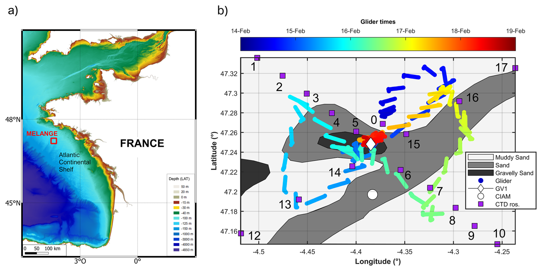
Figure 1 (a) The MELANGE campaign area, off the French Atlantic coast. Bathymetry from SHOM (2015); (b) SeaExplorer glider path with locations of CIAM (white disk) and GV1 (white diamond) moorings, and CTD-Rosette casts (purple squares), superimposed on the surface sediment composition of the ocean floor according to Garlan et al. (2018).

2.2 Sea conditions

The main hydrodynamic forcing in the validation area is the semi-diurnal tide, dominated by the M2 and S2 components (Vincent and Le Provost, 1988). During the validation campaign, the tidal range decreased from 3.9 to 2.5 m at the GV1 mooring (Fig. 2b). The south-to-north component v reached its extrema in the 5th hour before slack water (Fig. 2c). The west-to-east component u, 2 h approximately phase shifted, reached its extrema in the 2nd hour before slack water, with lower maxima than v (Fig. 2c). Consequently, the overall tidal current was maximal in the SSW-NNE directions, minimal in the orthogonal directions, and had magnitudes between 0.1–0.3 m s⁻¹.

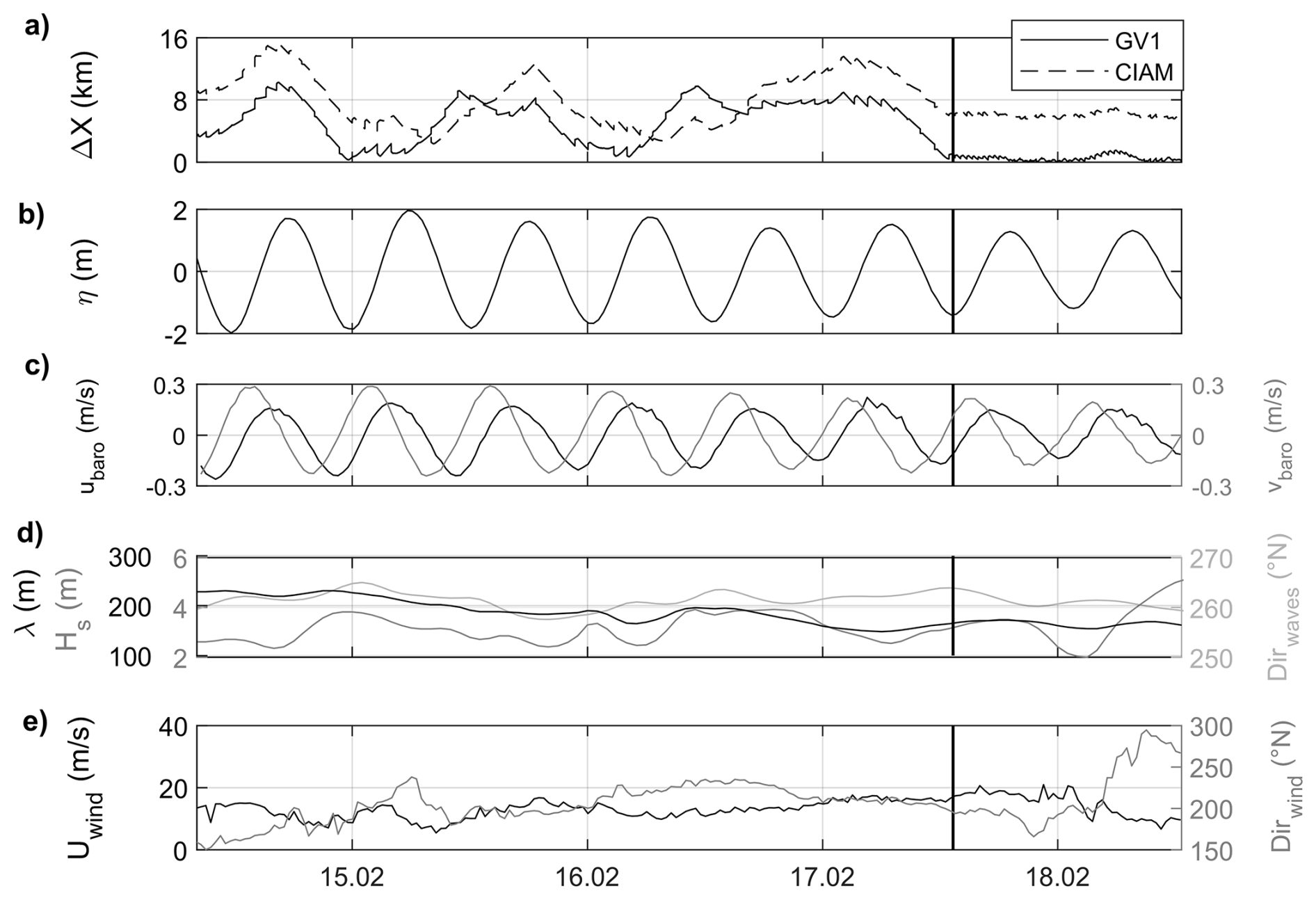
Figure 2 Environmental settings: (a) Glider-moorings geographic distance, (b) tidal elevation [m] from the GV1 ADCP pressure sensor, (c) tidal current components u and v from the GV1 ADCP (depth-averaged), (d) significant wave height, wavelength and direction estimated from the WAVEWATCH-III model from Ifremer (2022) at GV1 location, (e) wind speed and wind direction from RV Thalassa weather station. The black line delineates the Butterfly and Virtual Mooring survey periods (cf. Sect. 3.1).

The wave characteristics for the validation period, calculated with the WAVEWATCH-III wave generation and propagation model (Tolman, 2009) and interpolated at the GV1 mooring, show mean significant heights and wavelengths of 4 and 148 m, respectively, mostly coming from the west (Fig. 2d), and maximum values of 5 and 245 m, respectively. According to the meteorological equipment installed on RV (Research Vessel) Thalassa, the wind blew from the SSW, with a mean intensity of 12 m s⁻¹ and peaks up to 23 m s⁻¹ (Fig. 2e). The spatial extent of the validation area (∼10 NM) is small enough to consider that the physical parameters described in this paragraph (representative of larger-scale conditions, ∼30–60 NM) are homogeneous and thus valid across the entire study domain. Furthermore, the measurement period allowed us to sample 8 tidal cycles, i.e. 8 times the period of the dominant forcing, with variable amplitudes, enabling us to assess the performance of the glider over a representative period of the tidal forcing.

3 Materials

Figure 3 displays the scientific instrumentation used during the MELANGE campaign, corresponding to a measurement strategy that is exposed in Sect. 3.1. It first involves a glider (Sect. 3.2), two bottom moorings (Sect. 3.3) and a CTD-Rosette deployed from the research vessel entitled “La Thalassa” (Sect. 3.4). The dataset used in this study (Homrani et al., 2025) is publicly available on Zenodo.

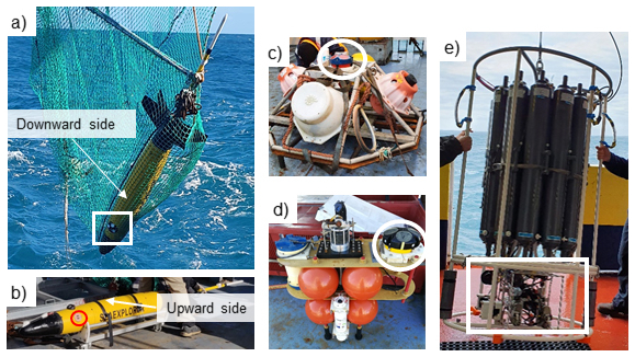
Figure 3 Scientific instrumentation used: (a) The SeaExplorer glider during its recovery, with the Nortek AD2CP current profiler (white rectangle); (b) The same glider with its Wetlabs FLBBCD probe including an optical backscattering sensor (red circle). (c) The CIAM upward-looking moored ADCP (white circle); (d) The GV1 upward-looking moored ADCP (white circle); (e) The CTD rosette, equipped with 11 Niskin bottles, a LISST-100X and a turbidity probe (in the white rectangle section).

3.1 Measurement strategy

During the first period of the campaign, lasting from 07:30 UTC 14 February to 13:20 UTC 17 February 2021, the glider navigated following a BUtterfly pattern (hereafter abbreviated BU) centred on GV1 (Fig. 1b). This pattern is relevant for comparing fixed measurements and glider measurements within a 10 NM scale, as it enables repeated sampling along two orthogonal transects, thereby improving spatial coverage and capturing both along- and cross-track variability (Bosse and Fer, 2019; Rollo et al., 2022; Cauchy et al., 2023). During BU the glider acquired more than 170 vertical profiles at distances less than 6 NM from GV1. For the remaining period, the glider performed a Virtual Mooring (hereafter called VM) with almost 45 profiles in much closer vicinity of GV1 (at 500±150 m from it), in order to acquire the most consistent data for comparison with this mooring. During the whole campaign, each glider profile lasted about 20 min allowing a sampling of each semidiurnal cycle with about 36 profiles. The glider vertical velocity is 0.2 m s⁻¹ on average.

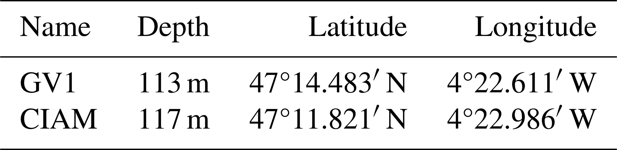
In order to evaluate the spatial consistency of the currents, a second ADCP was moored at a distance of about 3 NM south of GV1. This mooring, whose location is also displayed in Fig. 1b, is called CIAM, standing for “Châssis d'Instrumentation Autonome de Mesures”. The coordinates of the two moorings are given in Table 1.

Table 1 Locations of the two moorings (ITRF2014 geodetic system) with their Lowest Astronomical Tide (LAT) chart datum depths.

Finally, a CTD-Rosette sampler was deployed, performing an along-shelf section with 11 stations on 14 February and a cross-shelf section with 6 stations on 18 February (Fig. 1b). These CTD-Rosette casts, with in situ calibrated acquisitions based on water samples, are considered as the reference measurements for temperature, salinity, bio-optics with SPM measurements especially.

The glider, CIAM and the CTD-Rosette were deployed from RV Thalassa. GV1 was previously moored in January 2021, in the framework of ROEC/Benth.

3.2 Glider instrumentation

The ALSEAMAR SeaExplorer glider was equipped with a 1 MHz Nortek AD2CP Acoustic Doppler Current Profiler with a downward-looking configuration in the same way as in Pasqueron de Fommervault et al. (2019). The glider was programmed to dive with a pitch angle of approximately ±22°, with the design of the AD2CP allowing 3 beams in a optimal “Janus” configuration (Mullison, 2017) either for descents or ascents (Ma et al., 2019). The AD2CP compass is calibrated far from any magnetic disturbance to avoid biasing the current direction. In the present study, the calibration has been realized with the AD2CP mounted on the fully equipped glider, using the standard ALSEAMAR and Nortek (2022) procedures.

The AD2CP was configured to collect measurements in beam coordinates in 15 sampling cells, with a 2 m resolution and a 0.2 m blanking distance (Table 2). The profiler pinged 4 profiles per 1 s average ensemble, every 5 s. Bottom tracking was configured at the same sampling frequency, with a 0.1 m blanking distance, to detect the bottom position in the lowest ten meters of the water column. Velocities were acquired in beam coordinates.

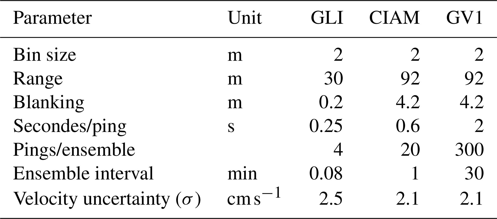
Table 2 Configurations of the downward-looking glider mounted AD2CP and the two upward-looking CIAM and GV1 moored ADCPs. The velocity uncertainty (last Table line) is the standard deviation error for both components (u and v) of the velocity profiles. The standard deviation values has been estimated in Sect. 4.5 for the glider and in Sect. 4.6 for the moorings.

To measure optical turbidity throughout the water column, the dry payload section of the SeaExplorer was also equipped with a Seabird WetLabs ECO-Puck FLBBCD sensor, which delivered light scattering measurements (expressed in m sr⁻¹) at a wavelength of 700 nm. A Seabird Glider-Pumped Conductivity, Pressure and Temperature probe (GPCTD), was also integrated into the nose of the SeaExplorer, to acquire ancillary hydrological measurements. The FLBBCD probe acquired optical backscattering every 1 s, and the GPCTD probe measured every 4 s.

3.3 Bottom moorings instrumentation

Each mooring contained an upward-looking RD Instrument ADCP, both operating at 300 kHz, each of them having four transducers forming 4 beams equally slanted with a 20° angle from the vertical direction. Table 2 specifies their configurations. Their vertical resolutions and ranges were identical but their temporal resolutions differed. CIAM ADCP was configured to acquire data with high temporal resolution as it had been specifically deployed for the MELANGE validation campaign. The temporal resolution of GV1 was lower (10 min measurements, averaged every 30 min) but it still allowed to collect data at a relevant timescale given the tidal periodicity of about 12 h. Compass calibration was performed on both ADCPs following the Le Menn and Pacaud (2015) procedure.

3.4 CTD-Rosette instrumentation

The CTD-Rosette sampler was notably equipped with a Seabird SBE911plus CTD and a WetLabs FLBBCD probe (same model as the glider), as well as being equipped with a Sequoia Scientific particle size analyzer (LISST-100X Type C) to measure volume distribution of suspended sediment in 32 size classes, logarithmically distributed from 2.5 to 500 µm (Agrawal and Pottsmith, 2000). We used the randomly shaped particle inversion method so that the final size classes used were centred from 2 to 350 µm with upper limits between 2.25–380 µm. Extreme size classes were removed because they showed typical “rising tails” explained by the presence of particles outside the measurement range of the instrument (Mikkelsen et al., 2005). Water samples were collected from the CTD-Rosette for analysis of suspended sediment concentration in particular.

4 Methods

The processing method used to recover the absolute currents recorded by an ADCP onboard a glider has been chosen as the well known “LADCP shear method” (Visbeck, 2002; Ordonez et al., 2012). This method is presented in Sect. 4.1, along with computation of the depth-averaged current components in Sect. 4.2 and fluxes in Sect. 4.3. Concerning SPMC, an ADCP is also able to recover an index of turbidity from the acoustic measurement following a method presented in Sect. 4.4. The assessment of the velocity uncertainties is given in Sect. 4.5, while for the moorings it is given in Sect. 4.6. Final errors given later in the results are computed according to metrics specified in Sect. 4.7. Contrary to the currents, the acoustic and the optical measurements of the particle concentrations need in situ calibrations. They are presented in Sects. 4.8 and 4.9.

4.1 Obtaining ocean currents with a glider-mounted ADCP

Processing of glider-AD2CP data is typically done at the end of a mission, once the full resolution dataset has been recovered. In the following Section we describe the main steps of the Delayed Mode algorithm. The AD2CP measurements take into consideration two contributions: the water current and the motion of the glider relative to the water body. To obtain the ocean contribution as a full water column profile, the LADCP shear method (Visbeck, 2002) was applied to each individual dive–climb cycle (hereafter yo) of the glider. Assuming that the velocity of the glider is constant during a ping (≈10 ms), and that the ocean current is stationary during a yo (≈20 min, see Sect. 4.6), the method is applicable to the AD2CP measurements U_AD2CP(z), such that:

$$\begin{array}{}\text{(1)}& {\displaystyle }{\displaystyle }{U}_{\text{AD2CP}}\left(z\right)=\left(U_{\text{barotropic}}+U_{\text{baroclinic}}\left(z\right)\right)+U_{\text{GLI}}\left(z\right)\end{array}$$

where U_GLI is the glider velocity relative to the water mass, U_barotropic and U_baroclinic are the depth-averaged (barotropic) and depth-varying (baroclinic) ocean current components, respectively, so that the total ocean current is $U_{\text{ocean}}\left(z\right)=U_{\text{barotropic}}+U_{\text{baroclinic}}\left(z\right)$. Based on Eq. (1), and treating u (east-west) and v (north-south) components separately, we then: (i) computed elementary shear profiles using central differences; (ii) averaged overlapping shears; and (iii) retrieved ocean currents by integrating shears, using the ocean velocities from the bottom track as the integration constant (Gentil et al., 2020). As the bottom track shows no variability with respect to sediment type or glider heading, it has been selected as a reference for constraining the relative velocity profiles.

Quality controlled tests are detailed in Pasqueron de Fommervault et al. (2019). The main pipeline of operations is set up:

1. to correct the speed of sound using the salinity and temperature measured by the glider;

2. to discard data with less than 50 % correlations or less than 3 dB signal-to-noise ratios;

3. to discard data when the glider is pitched or rolled enough to displaced cells from their nominal alignment (threshold of 20° around the nominal position);

4. to discard data out of the water column;

5. to discard outliers for which vertical shear velocity exceeds 0.02 s⁻¹;

6. to discard data farther away from the ADCP that are not consistent with those coming from profiles in close vicinity (Todd et al., 2011);

7. to discard data where vertical velocities in two adjacent cells during a ping exceeds the threshold of 0.05 m s⁻¹ (Visbeck, 2002);

8. to discard profiles with too many missing or extrapolated values;

9. to compute the mean shear in each depth interval only where more than 5 remaining (good) values are available.

The final measurements obtained were given as profiles with 2 m cells.

4.2 Computing depth-averaged velocities

The semi-diurnal tide is the main hydrodynamic forcing on the MELANGE area (Vincent and Le Provost, 1988). Accordingly, the measured ocean current was analysed from two perspectives: (i) the total current, that is, the current varying with both depth (cell) and time (profile), and (ii) the depth-independent current computed as the depth-averaged current, which we approximated as the tidal current due to being mostly driven by tide. The bottom boundary layer was estimated to be approximately 9–14 m thick during the 5 d campaign, using the Soulsby (1983) formula for tidal flows. Bottom depth varied over time along the glider track (−121 to −105 m) as the glider moved across spatially varying bathymetry. In order to compare a consistent barotropic layer of the water column for the three current profilers, given their respective deployment depth, data availability near the surface, and time-varying excursion of the tidal boundary layer from the seafloor, the depth-average was calculated for u and v separately as:

$$\begin{array}{}\text{(2)}& {\displaystyle }{\displaystyle }{u}_{\mathrm{t}}\left(t\right)=\underset{-\mathrm{98}\mathrm{m}}{\overset{-\mathrm{52}\mathrm{m}}{\int }}u(t,z)\mathrm{d}z\end{array}$$

with t the time of the glider-AD2CP profile and z the depth computed from the free surface. The value 98 m is the minimum of the difference between the ocean depth recorded (typically 110 m) and the thickness of the bottom boundary layer (typically 12 m) computed using the Soulsby (1983) formula. The value 52 m corresponds to the maximum range of the CIAM ADCP recorded at the end of the survey, as seen in Fig. 6. In the MELANGE area (of size ∼10 NM), the tidal range is considered spatially homogeneous, as it operates on a larger scale than the studied area. Therefore, the depths of the current profiles are given hereafter with respect to the tide-varying free surface position, rather than with respect to the space and time-varying bathymetry.

4.3 Computing suspended sediment fluxes

The instantaneous flux of SPM, at all depths and locations of geographic points surveyed, notated Q_F, and the flux integrated in depth, notated Q_S, with their two components u and v, are calculated separately as follows:

$$\begin{array}{}\text{(3)}& {\displaystyle }\begin{array}{rl}{\displaystyle }{Q}_{\mathrm{S}u}\left(t\right)& {\displaystyle }={\int }_{z\left(\text{bottom}\right)}^{z\left(\text{surface}\right)}{Q}_{\mathrm{F}u}(t,z)\mathrm{d}z\\ {\displaystyle }& {\displaystyle }={\int }_{z\left(\text{bottom}\right)}^{z\left(\text{surface}\right)}\text{SPMC}(t,z)\cdot u(t,z)\mathrm{d}z\\ {\displaystyle }{Q}_{\mathrm{S}v}\left(t\right)& {\displaystyle }={\int }_{z\left(\text{bottom}\right)}^{z\left(\text{surface}\right)}{Q}_{\mathrm{F}v}(t,z)\mathrm{d}z\\ {\displaystyle }& {\displaystyle }={\int }_{z\left(\text{bottom}\right)}^{z\left(\text{surface}\right)}\text{SPMC}(t,z)\cdot v(t,z)\mathrm{d}z\end{array}\end{array}$$

where t the time of the glider-AD2CP profile, u and v the two velocity components and z the depth from the bottom ocean to its surface. Because the glider reverses its trajectory when approaching an interface, there are missing data during those phases. Consequently, at a usual distance of about 8 m from the ocean bottom and 16 m from the ocean surface, data are lacking. The missing data (u,v) and SPMC located near the bottom and the surface are completed by extrapolation, repeating the closest value recorded near the interface.

4.4 Obtaining acoustic backscatter from ADCP data

Acoustic backscatter values were also obtained from the glider-AD2CP profiler and provided an additional (acoustic related) proxy of the suspended sediment concentration (Thorne and Hanes, 2002). The acoustic backscatter S_v (dB], also referred to as volume backscattering strength in the literature, is a metric of the acoustic signal returned by the scatterers in a finite cell-size volume. As in optics, the acoustic backscatter is linked to particulate abundance, and therefore to concentration, but also to particle size as well as to shape and mechanical contrasts with the surrounding fluid, see e.g. Stanton, 1989; Pieper and Holliday, 1984. In the present work, S_v (dB] is computed from the echo amplitude E [counts], i.e. the raw output values given by the AD2CP, as follows Jourdin et al., 2014; Nortek, 2022:

$$\begin{array}{}\text{(4)}& \begin{array}{rl}& S_{\mathrm{v}}=\text{RL}+\mathrm{2}\text{TL}+\text{DT}-\text{SL}-\mathrm{10}{\log }_{\mathrm{10}}\left(V\right)\\ & \text{RL}=\mathrm{10}{\log }_{\mathrm{10}}\left({\mathrm{10}}^{K_{\mathrm{c}}\cdot (E-E_{\mathrm{0}})/\mathrm{10}}-\mathrm{1}\right)\\ & \text{TL}=\mathrm{20}{\log }_{\mathrm{10}}\left(\mathit{\psi }R\right)+{\mathit{\alpha }}_{\mathrm{w}}R\\ & V=\mathit{\varphi }\cdot {\left(\mathit{\psi }R\right)}^{\mathrm{2}}\cdot {\displaystyle \frac{c\mathit{\tau }}{\mathrm{2}}}\end{array}\end{array}$$

The reverberation level RL is calculated according to the formula by Mullison (2017), after Gostiaux and van Haren (2010), with E₀ [counts] the echo noise floor and K_c [$\mathrm{dB}/\mathrm{count}$] the conversion slope. Transmission loss TL is calculated using the range of acoustic cells from transducers R, associated with near-field correction ψ (Downing et al., 1995) and the coefficient of sound absorption α_w (dB m⁻¹]. Our calculation takes into account the contribution of water only, through the formula given by Francois and Garrison, 1982: we consider the absorption by suspended particles to be negligible given their low concentrations (cf. Sect. 5.2.1) far less than 100 mg L⁻¹ (Tessier et al., 2008). SL and DT [dB] represent the Sound Level emitted by the instrument, and its Detection Threshold, respectively set to 217 and 100 dB (Nortek AS, personal communication, 2021). The velocity of sound in water c [m s⁻¹] is set to 1500 m s⁻¹. The volume of an acoustic cell V can be estimated with τ [s], the pulse duration of the acoustic signal, equal to 2.94 ms for our instrument and ϕ the solid beam angle [sr] corresponding to an aperture angle of 2.9°.

Only the two beams that point to the sides (Beams 2 and 4) are selected for the final computation of the backscatter profile, because these beams are always oriented downwards, whether the glider dives up or down. Then, for each bin, we take the minimum value of the two backscatter values recorded, in order to discard possible scattering outliers. In the following analysis, acoustic data recorded in near-surface layers of the ocean (from 0 to 20 m depth) were discarded due to the very noisy accompanying backscatter signal. This is most likely the result of contamination by air bubble clouds which act as high-strength scatterers (Van Haren, 2001). The presence of air bubbles, which are created at the air-water interface and advected downward, is related to rough wind and wave conditions (Wang et al., 2011; Vagle et al., 2010), that occurred during the present campaign (cf. Fig. 2).

4.5 Uncertainty assessment of glider AD2CP velocities

To validate the current estimates, the AD2CP measurement uncertainty for the reconstructed profiles has to be considered. For the Nortek 1 MHz instrument integrated on the SeaExplorer and cells with a resolution of 2 m, the manufacturer specifies a typical ping uncertainty of approximately 6 cm s⁻¹ (the same as for the bottom track ping). The instrument sampled continuously at 4 Hz and recorded 5 s ensemble averages composed of 20 pings, yielding a precision of approximately 3 cm s⁻¹ for each ensemble beam velocity (Table 2). Given the 5 s averaging interval and a typical glider vertical velocity of 0.2 m s⁻¹, the number of overlapping measurements per 2 m cell ranges from 1 near the surface to about 30 over most of the profile. By discarding cells with less than 3 overlaps and propagating independent errors, both due to water pings (WP) and bottom track (BT) pings, the uncertainty on horizontal velocities is computed as:

$$\begin{array}{}\text{(5)}& {\displaystyle }{\displaystyle }{\mathit{\sigma }}_{\text{GLI}}=\sqrt{{\left({\displaystyle \frac{{\mathit{\sigma }}_{\text{WP}}}{\sqrt{N}}}\right)}^{\mathrm{2}}+{\left({\displaystyle \frac{{\mathit{\sigma }}_{\text{BT}}}{\sqrt{N}}}\right)}^{\mathrm{2}}},\end{array}$$

with ${\mathit{\sigma }}_{\text{WP}}={\mathit{\sigma }}_{\text{BT}}=\mathrm{3}$ cm s⁻¹, and N the number of overlapping samples per cell. In the worst-case scenario (N=3), this yields σ_GLI≈2.5 cm s⁻¹. This value is lower than the uncertainties reported in similar high-frequency glider deployments in coastal settings, typically around 4 cm s⁻¹ (Ma et al., 2019).

4.6 Uncertainty assessment of moored ADCP velocities

First, a quality-control filtering was performed, based on standard recommendations (Gordon and RDI, 1996): cells with (i) a range above the maximum range predicted by PlanADCP, (ii) a beam correlation lower than 64 counts, (iii) a sum of the percents good of beams 1 and 4 lower than 75 %, and (iv) an absolute error velocity higher than 6 cm s⁻¹, were discarded. For the CIAM data, the profiles, available every minute, were averaged over the glider profile's inherent averaging period. This averaging also allows computation of corresponding standard deviations for the CIAM horizontal velocities. Hence, a typical standard deviation error σ(CIAM)=2.1 cm s⁻¹ for both components of the horizontal velocities has been estimated, knowing that this standard deviation encompasses not only measurement errors but also the ocean variability at the averaging scales used, over the vertical and in time with O(30 min). For the GV1 data (10 min of measurements averaged every 30 min), we assumed a similar standard deviation value of σ(GV1)=2.1 cm s⁻¹ knowing that the two ADCPs were similarly configured and moored in the same area, with averaging timescales of O(10–20 min) for GV1.

4.7 Further error metrics

ADCP data from the GV1 and CIAM moorings were post-processed in order to match the AD2CP data characteristics of the glider acquisitions. ADCP-AD2CP vertical cells were paired without interpolation when their centre depths differed by less than 1 m. The vertical positions of the cells were then expressed with respect to the free surface (which is the pressure reference for the glider), using the ADCPs' integrated pressure sensors. Finally, glider and mooring profiles were temporally paired by selecting the closest ADCP profiles in time. As said in the previous Section, CIAM data were averaged over the glider profile's inherent averaging period. For the GV1 data, the closest profiles to the glider profiles within a 30 min interval were used. To ensure reliable statistical comparisons between platforms, cells with less than 20 % of overlaps throughout the averaging period, due to failed quality controls, were discarded.

For current comparisons, bias and Root Mean Squared Differences (RMSD) are computed as follows:

$$\begin{array}{}\text{(6)}& {\displaystyle }\begin{array}{rl}\text{bias}& =\text{bias}\left(X\right)\\ & ={\displaystyle \frac{\mathrm{1}}{N}}\sum _{i=\mathrm{1}}^{N}X(\text{Platform2}{)}_i-X(\text{Platform1}{)}_i\end{array}\text{(7)}& {\displaystyle }\begin{array}{rl}\text{RMSD}& =\text{RMSD}\left(X\right)\\ & =\sqrt{{\displaystyle \frac{\mathrm{1}}{N}}\sum _{i=\mathrm{1}}^N{\left(X(\text{Platform2}{)}_i-X(\text{Platform1}{)}_i\right)}^{\mathrm{2}}}\end{array}\end{array}$$

where X is one velocity component; Platform1 and Platform2 can be either GLI, CIAM or GV1; i indicates a common bin cell and N is the total number of bin cells considered in the comparison.

In order to compare the RMSD obtained (in Sect. 5.1.1) with the a priori error estimations performed in previous Sects. 4.5 and 4.6, a Combined Uncertainty (CU) has also been defined as follows:

$$\begin{array}{}\text{(8)}& \text{CU}=\sqrt{{\mathit{\sigma }}^{\mathrm{2}}\left(\text{Platform1}\right)+{\mathit{\sigma }}^{\mathrm{2}}\left(\text{Platform2}\right)}\end{array}$$

where σ is the standard deviation that typically is worth 2.5 cm s⁻¹ for the glider and 2.1 cm s⁻¹ for the moorings. With this definition of CU we assume that errors coming from different platforms are uncorrelated.

Concerning suspended matter, the Root Mean Squared Log Differences (RMSLD) and Relative Percent Difference (RPD) are used:

$$\begin{array}{}\text{(9)}& {\displaystyle }\begin{array}{rl}& \text{RMSLD}=\text{RMSLD}\left(Y\right)\\ & =\sqrt{{\displaystyle \frac{\mathrm{1}}{M}}\sum _{j=\mathrm{1}}^M({\log }_{\mathrm{10}}\left(Y(\text{System2}{)}_j\right)-{\log }_{\mathrm{10}}\left(Y(\text{System1}{)}_j\right){)}^{\mathrm{2}}}\end{array}\text{(10)}& {\displaystyle }\begin{array}{rl}\text{RPD}& =\text{RPD}\left(Y\right)\\ & =\mathrm{100}\cdot {\displaystyle \frac{\mathrm{1}}{M}}\sum _{j=\mathrm{1}}^M{\displaystyle \frac{\left|Y\right(\text{System2}{)}_j-Y\left(\text{System1}{)}_j\right|}{Y(\text{System1}{)}_j}}\end{array}\end{array}$$

where Y is SPMC or a backscattering intensity; System1 and System2 are measurement systems such as filter weighing, optical or acoustic backscattering, where System1 is considered as a reference; j identifies one pair of compared measurements, with M being their total number.

4.8 In situ SPMC calibration of the optical sensors

The glider-mounted WetLabs BB700 optical backscattering sensor outputs were converted from volume scattering measurements into optical particulate backscattering coefficients b_bp [m⁻¹] as proposed by Schmechtig et al. (2018) and Boss and Pegau (2001), using the temperature and salinity concomitantly measured by the GPCTD of the glider to remove the water backscattering contribution (Zhang et al., 2009). The outputs of the CTD-Rosette-mounted WetLabs BB700 optical backscattering sensor (same sensor model and wavelength) were processed identically.

In order to obtain a direct ground estimation of the SPMC (in [mg L⁻¹]), the water samples collected with the CTD-Rosette sampler were filtered, and the corresponding filters were weighted following a standard procedure based on triplicates, e.g. Neukermans et al. (2012). SPMC measurements from filtrations were used to calibrate the CTD-Rosette optical scattering acquisitions, in order to retrieve SPMC from the latter. To do so, the optical measurements acquired when the Niskin bottles were closed (6 measurements) were averaged. The corresponding means were linearly fitted with SPMC values obtained from filtration, taking the log ₁₀ of the two parameters to perform the fit in order to improve the statistical estimation (Fig. 4).

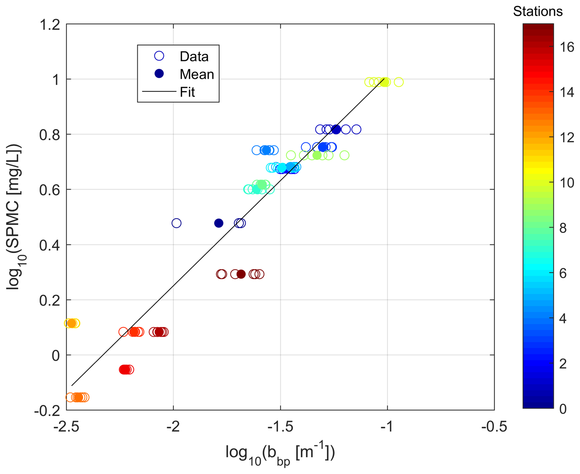
Figure 4 Calibration between the optical particulate backscattering coefficients b_bp, and the Suspended Particulate Matter Concentrations (SPMC), measured with the CTD-Rosette on 17 stations (see locations in Fig. 1). Data correspond to the bottom measurements, with three to six b_bp values for one SPMC value; Mean is the mean b_bp value on this three to six b_bp measurements; Fit is obtained by linear regression (p value $<{\mathrm{10}}^{-\mathrm{8}}$), spelled out in Eq. (11).

The calibration equation was taken for the best coefficient of determination (R²=0.91), obtained when combining the 14 and 18 February 2021 datasets for the bottom measurements, and also leads to the following RMSLD and RPD error values (filter weighing being the reference):

$$\begin{array}{}\text{(11)}& \begin{array}{rl}& {\log }_{\mathrm{10}}\left(\text{SPMC}\right)=\mathrm{0.8}\times {\log }_{\mathrm{10}}\left(b_{\text{bp}}\right)+\mathrm{1.8}\\ & R^{\mathrm{2}}=\mathrm{0.91}\\ & \text{RMSLD}\left(\text{SPMC}\right)=\mathrm{0.11}{\log }_{\mathrm{10}}\left(\mathrm{mg}{\mathrm{L}}^{-\mathrm{1}}\right)\\ & \text{RPD}\left(\text{SPMC}\right)=\mathrm{17}\mathrm{\%}\end{array}\end{array}$$

Bottom data giving the best fit is consistent with numerous observations reported in the literature, as seen for example in Fettweis et al. (2019). Combining the 14–18 February datasets has the advantage of providing a calibration equation that is valid over the full campaign duration. Nonetheless, from the dispersion of some points in Fig. 4, it looks like there are some unresolved dependency on site, i.e. bottom sediment type. Then some variability in the relation can probably be due to seabed sediment type variation not included in the regression.

Also this SPMC calibration is valid only for the optical sensor onboard the CTD-Rosette (carrying the Niskin bottles used in this in situ calibration). The optical sensor onboard the glider is of same model and wavelength as the one onboard the CTD-Rosette, but its last laboratory calibration was carried out on 8 July 2015, while the sensor onboard the CTD-Rosette was calibrated in laboratory on 8 January 2021, only a month ahead of the sea survey. By default we applied the same calibration equation to the optical sensor onboard the glider. However, errors in the laboratory calibration of the glider sensor may propagate through the in situ calibration law and result in additional SPMC errors.

4.9 In situ SPMC calibration of the glider-AD2CP

Acoustic and optical backscatter coefficients recorded from the glider were compared each other in order to derive a correlation law. For pairwise comparison along the vertical, each acoustic backscatter value compared is the median of all values recorded in beam profiles that were stacked at the same vertical height. The final resolution on the vertical being 2 m (the size of each ADCP bin), the typical distance of comparison between optical and acoustic values is of the order of 1 m.

Figure 5 shows the correlation between optical and acoustic backscattering coefficients in the deep layer. Such correlation is expected for suspended sediment particles of mineral origin (Tessier et al., 2008). To ensure consistency, the surface layer was excluded from the regression, as micro-bubbles and plankton can alter the acoustic-to-optical response and introduce strong variability (Jourdin et al., 2014). The resulting calibration (S_v, b_bp), representative of the full MELANGE period, is given by:

$$\begin{array}{}\text{(12)}& \begin{array}{rl}& {\log }_{\mathrm{10}}\left(b_{\text{bp,Gli}}\right)=\mathrm{0.07}\times S_{\mathrm{v}}+\mathrm{0.2}\\ & R^{\mathrm{2}}=\mathrm{0.88}\\ & \text{RMSLD}\left(b_{\text{bp,Gli}}\right)=\mathrm{0.09}{\log }_{\mathrm{10}}\left({\mathrm{m}}^{-\mathrm{1}}\right)\\ & \text{RPD}\left(b_{\text{bp,Gli}}\right)=\mathrm{15}\mathrm{\%}\end{array}\end{array}$$

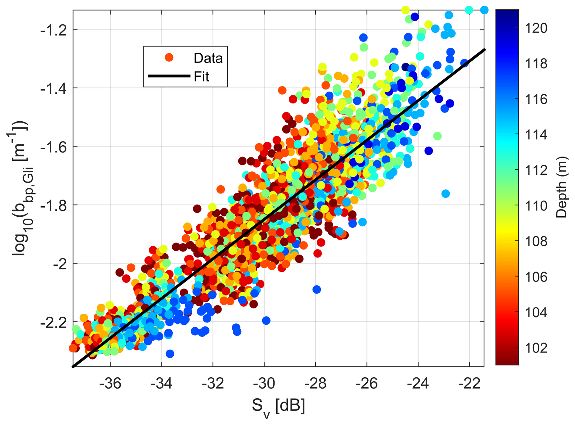
Figure 5 Calibration between the optical particulate backscatter coefficients b_bp and the acoustic backscatter of the AD2CP S_v measured by the glider in the deep layer. Data correspond to the glider measurements (N = 2547). Fit is obtained by linear regression (p value $<{\mathrm{10}}^{-\mathrm{10}}$), spelled out in Eq. (12).

Note that converting Eq. (12) from logarithmic to linear units increases the relative spread of the uncertainty and skews the resulting distribution, even if no additional error is formally introduced. This effect is discussed in Edge et al. (2021), their Fig. 12.

We propose here to calibrate in situ the turbidimeter (backscattering sensor) onboard the glider, using the same calibration equation (Eq. 11) obtained for the turbidimeter onboard the CTD-Rosette, even though the former laboratory calibration was performed at a distant date (see Sect. 4.8). Combining this equation with the previous Eq. (12) leads to an estimation of the SPMC from the glider S_v according to the following new equation (with propagation of errors reported below, assuming independent regression models):

$$\begin{array}{}\text{(13)}& {\displaystyle }\begin{array}{rl}{\displaystyle }& {\displaystyle }{\log }_{\mathrm{10}}\left(\text{SPMC}\right)=\mathrm{0.06}\times S_{\mathrm{v}}+\mathrm{2.0}\\ {\displaystyle }& {\displaystyle }\text{RMSLD}\left(\text{SPMC}\right)=\mathrm{0.13}{\log }_{\mathrm{10}}\left({\mathrm{m}}^{-\mathrm{1}}\right)\\ {\displaystyle }& {\displaystyle }\text{RPD}\left(\text{SPMC}\right)=\mathrm{21}\mathrm{\%}\end{array}\end{array}$$

Finally, for the same reason as in Sect. 4.8 (distant date of laboratory calibration), this estimation of SPMC may include a bias.

5 Results and Discussion

In assessing suspended particulate transport and quantifying hydro-sedimentary processes (presented in Sect. 5.3), the glider needs the ability to sufficiently measure both the general currents (presented in Sect. 5.1) and the suspended particulate concentrations (presented in Sect. 5.2).

5.1 Validation of Glider currents

In this Section, the total currents are first presented (Sect. 5.1.1) and also their depth-averaged components (Sect. 5.1.2), knowing that the water column appeared to be homogeneous in terms of density (temperature and salinity) during the sea survey (not shown here).

5.1.1 Total current

Figure 6 shows that the two current components observed by all platforms display similar patterns and intensities, with a consistent tidal current periodic signal (with M2 the main tidal component with a period of 12 h 25^′). However, we can see sometimes differences in strength between GLI and the moorings, especially near the ocean surface. This comparison relies on the assumption that the spatial variability of the ocean current, at the scale of the MELANGE area, is not significant compared to its temporal variability under tidal forcing.

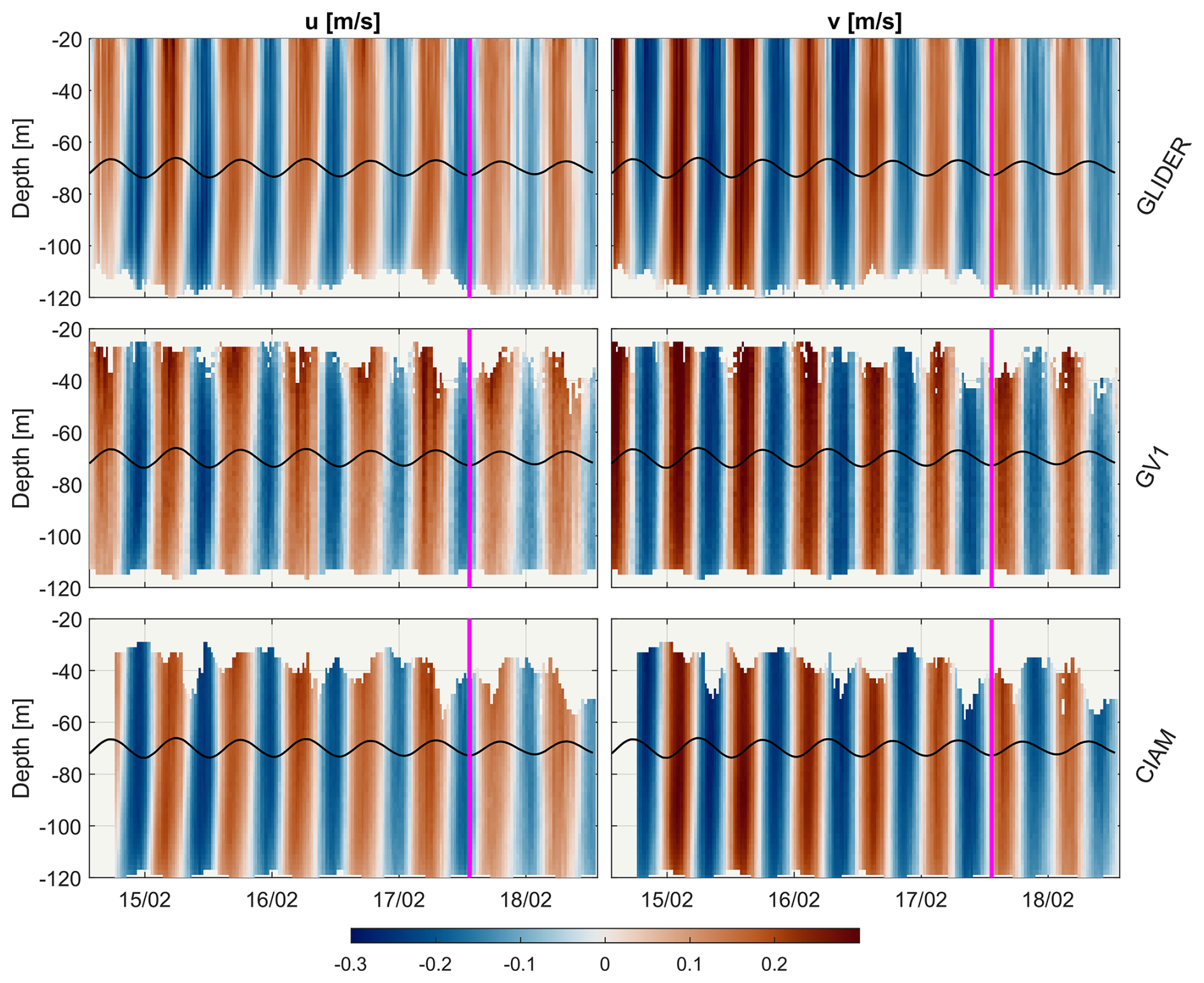
Figure 6 Current components measured by the glider-AD2CP and moored ADCPs from GV1 and CIAM. For glider data, bottom depth evolves with trajectory. Deepest measurements follow the bottom at a distance of about 8 m. Missing data near the bottom (usually less than 8 m) result from reversing of the glider trajectory near the seafloor. GV1 missing data near the bottom is due to the higher position of the ADCP relative to the seafloor compared to CIAM. Moorings' missing data close to the surface correspond to the maximum detection range of the ADCPs. The black line represents the free surface variation with tide (put in the middle of the graphic for a better display), computed from the GV1 pressure sensor. The vertical magenta line delineates the BU and VM survey periods.

To evaluate whether spatial variability is negligible compared to temporal variability, we compared the current measurements from the two moorings (Fig. 7a). The root-mean square difference (RMSD) between the two components ranges from 2.4 to 3.1 cm s⁻¹, which corresponds to about 10 % of the maximum observed current (0.3 m s⁻¹), and is consistent with the Combined Uncertainty (CU) of O(3 cm s⁻¹) between CIAM and GV1 (Table 3). In addition, the high determination coefficients (R²>0.95, $p<{\mathrm{10}}^{-\mathrm{6}}$) indicate that the two moorings capture very similar temporal variability. Together, the low RMSD and high R² support the assumption that spatial differences are minimal during the deployment period, and that both moorings provide consistent measurements of the tidal signal across the study area.

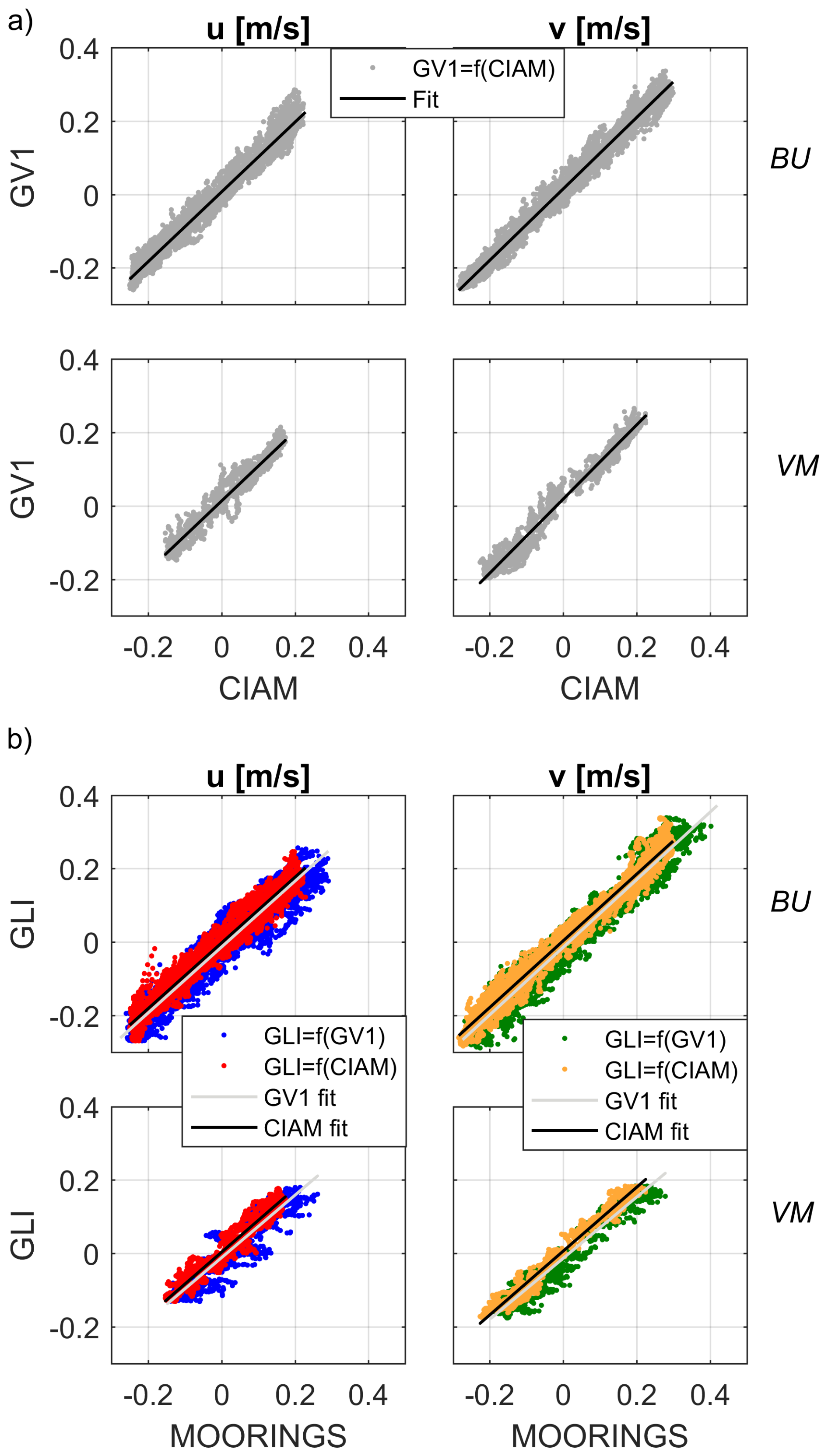
Figure 7 Total current linear regressions for u and v current components: (a) CIAM vs. GV1 moorings comparison; (b) Glider vs. CIAM and GV1 moorings comparison. Subplots distinguish BU and VM data. Associated regression coefficients (p values $<{\mathrm{10}}^{-\mathrm{6}}$) are given in Table 3.

Table 3 Comparison of ADCP horizontal velocity components (u and v) recorded from two different platforms. Indexes BU and VM respectively stand for the BUtterfly-pattern and Virtual-Mooring survey periods. Determination coefficients R² and bias (cm s⁻¹) are obtained after linear regression between the velocity components from the two compared platforms, also with RMSD (cm s⁻¹) from Eq. (7) and Combined Uncertainties (CU) from Eq. (8). All regression p values are lower than 10⁻⁶, meaning the affine-linear relationship is significant. Nota bene: CU values varies slightly depending on the considered component and period of comparison.

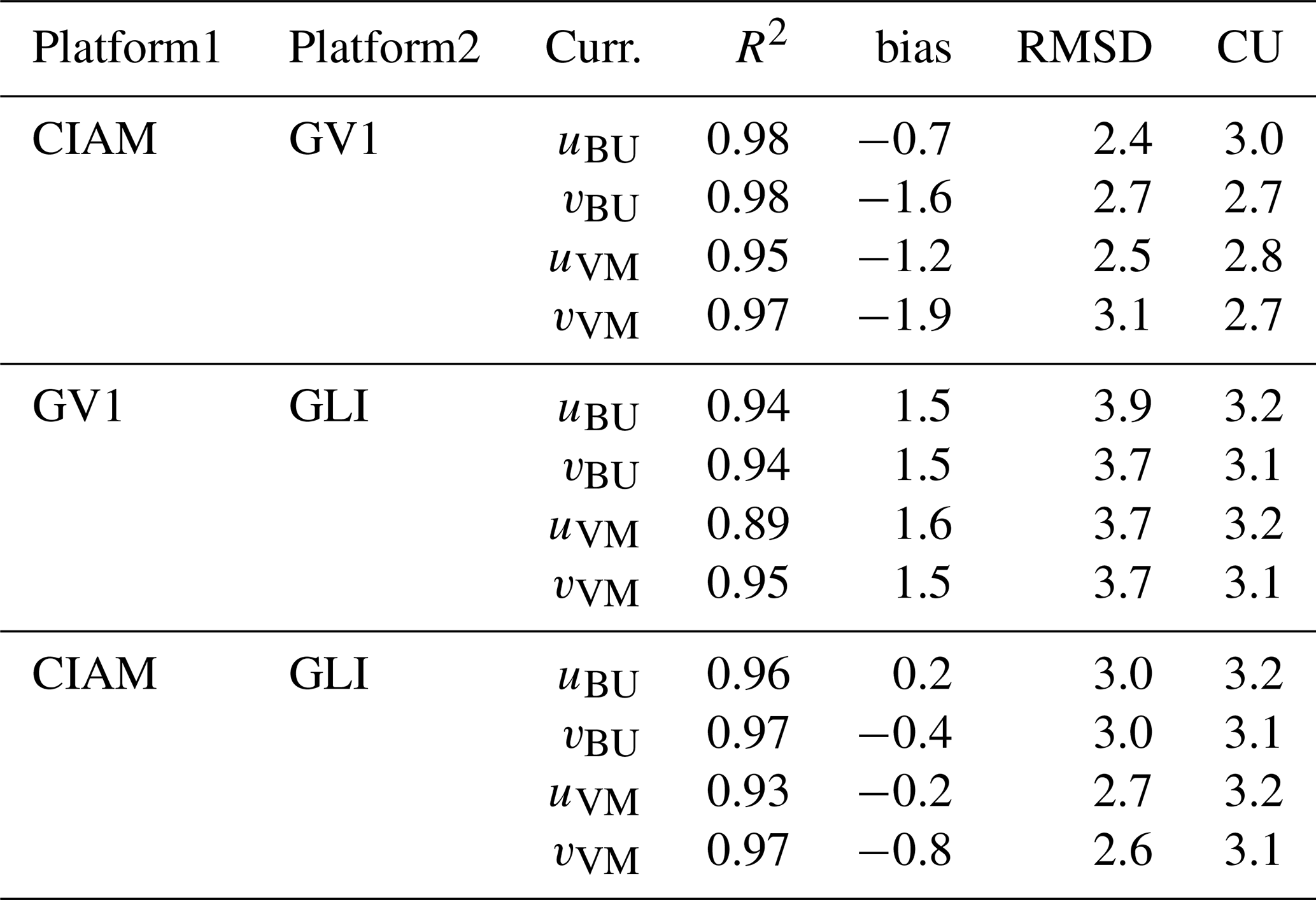
The RMSD between GLI and CIAM is around 3 cm s⁻¹, well within the CU, indicating a strong consistency between glider and mooring measurements. The RMSD with GV1 is slightly higher (4 cm s⁻¹), exceeding the CU by only 0.5–0.7 cm s⁻¹ (Table 3). This modest difference may reflect local flow variability or residual uncertainty associated with the glider's shear-based current reconstruction. This method involves integrating vertical shear over individual yos spanning 25 min and 500 m horizontally, which may challenge the assumption of steady flow during periods of strong tidal variability, such as spring tides (Todd et al., 2017). Despite these factors, the RMSD values remain fully consistent with previous glider validation studies using bottom-track referencing – an approach known to yield the lowest uncertainties (Thurnherr, 2010; Ordonez et al., 2012; Ellis et al., 2015). In all cases, determination coefficients (R²) remain high (0.93–0.97), confirming that the temporal variability is consistently captured across platforms.

Values of biases in Table 3 are larger when GV1 is compared to other platforms. These biases are negative when comparing CIAM with GV1, and positive when comparing GV1 with GLI. This suggests a systematic and oriented shift in the measurements made by the ADCP mounted on GV1. Such a shift might be attributed to the proximity of GV1 to the shipwreck Erika (GV1 is a long term mooring, that is usually put near shipwrecks in order to avoid bottom trawling) potentially causing a minor deviation of its compass. The result is a significant contribution of these large biases to the RMSD values, even during the VM period when the two platforms GV1 and GLI were close together (nearly at the same point). By opposition, biases between CIAM and GLI are smaller, but RMSD values remain at almost 3 cm s⁻¹ during the VM period, even though the two platforms CIAM and GLI were separated by a larger distance of about 3 NM during that period.

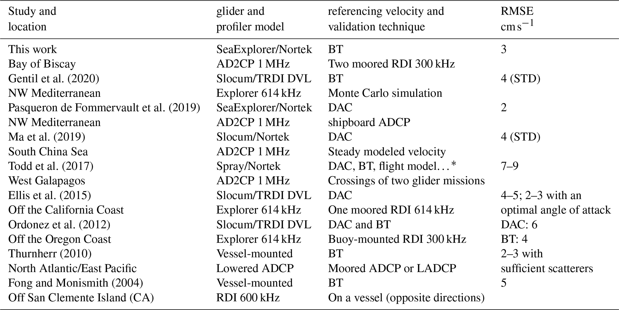
Nevertheless, these results match the values reported in the literature with in situ validations for a wide variety of well-documented deployment and settings of gliders (Table 4). In particular, the mean RMSE of comparison between GLI (glider) and CIAM (mooring) round 3 cm s⁻¹ is in agreement with those obtained in studies also using bottom track referencing, an approach yielding to the lowest uncertainties compared e.g. to dive-averaged referencing (Thurnherr, 2010; Ordonez et al., 2012), either obtained for an optimized angle of attack (Ellis et al., 2015), or for the ideal case of sufficient scatterers in suspension (Thurnherr, 2010).

Gentil et al. (2020)Pasqueron de Fommervault et al. (2019)Ma et al. (2019)Todd et al. (2017)Ellis et al. (2015)Ordonez et al. (2012)Thurnherr (2010)Fong and Monismith (2004)

Table 4 Literature review of the uncertainty (RMSE, cm s⁻¹) obtained in depth-resolved absolute current measured from gliders or vessels. Studies presented here all use the shear method (Visbeck, 2002) to compensate for the glider's motion, except Todd et al. (2017), who uses the inverse method. BT stands for bottom track, DAC for dive-averaged current.

^* see the article by Visbeck (2002) for all the constraints used.

5.1.2 Depth-averaged current

In theory, a purely barotropic tidal flow should vary in time but remain vertically uniform. To evaluate the glider's ability to capture this barotropic flow, we focus herein on the depth-averaged horizontal velocity between 52–98 m (see Sect. 4.2). This depth range was selected to avoid surface and bottom layers, where non-linear processes such as wind forcing, wave–current interactions (Signell et al., 1990; Müller et al., 1986), or bottom friction can alter the vertical structure of the flow (Grant and Madsen, 1986; Soulsby, 1983; Rippeth et al., 2003; Inall et al., 2021).

Figure 8 shows that the depth-averaged current components reach ±0.2 m s⁻¹ for u_t and ±0.3 m s⁻¹ for v_t. Across all current profilers, these components account for nearly all of the total flow (ratio ≈1), which is consistent with a predominantly barotropic tidal signal. The comparison between platforms confirms the accuracy of the glider-derived depth-averaged current. RMSD are consistently around 2 cm s⁻¹ for all components and periods, which represents roughly 10 % of the typical tidal amplitude. R² range from 0.93 to 0.98 (p values $<{\mathrm{10}}^{-\mathrm{10}}$), reflecting a strong temporal coherence between the glider-derived and mooring measurements. Similar statistics are found between the two moorings themselves. The largest discrepancies, up to 6 cm s⁻¹, occur near the tidal maxima: 2 h before high tide for u_t and 4 h before for v_t (Fig. 8). These peaks coincide with spring tide periods, when velocity gradients evolve rapidly. Under such conditions, the steady-state flow assumption – implicit in the glider's shear-based reconstruction over 25 min and 500 m horizontally – may not strictly hold, as discussed in Sect. 5.1.1.

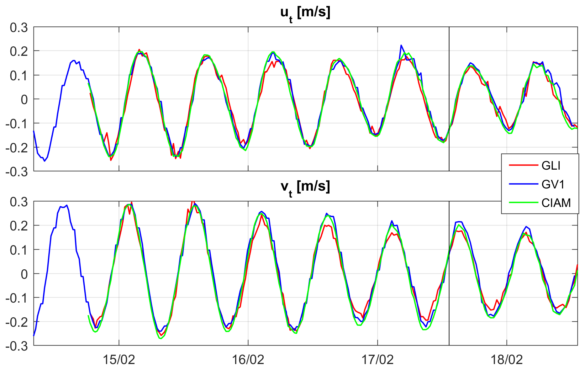
Figure 8 Depth-averaged current components computed from Eq. (2), for the glider-AD2CP (GLI) and moored-ADCPs (CIAM, GV1). The vertical black line delineates the BU and VM survey periods.

As previously mentioned, the tidal flow in the ocean is not strictly vertically uniform, due to nonlinear processes. To quantify such vertical deviations from the depth-averaged flow, we compute the residual field defined as $u(z,t)-\stackrel{\mathrm{‾}}{u}\left(t\right)$, where $\stackrel{\mathrm{‾}}{u}\left(t\right)$ is the depth-averaged velocity. This vertical residual from the depth-averaged flow isolates both instrumental artefacts and possible nonlinear processes. Figure 9 displays this residual for the glider and CIAM data, which offers the highest temporal resolution. While residuals are generally weak (<0.02 m s⁻¹), enhanced differences are observed near the surface and bottom, reaching up to 0.06 m s⁻¹. These depths correspond to the glider's dive and apogee phases, where fewer overlapping measurements are available (typically three after quality control), resulting in noisier profiles and likely contributing to the observed discrepancies. However, quality control alone cannot explain the observed differences, as they are more pronounced near the bottom than at the surface.

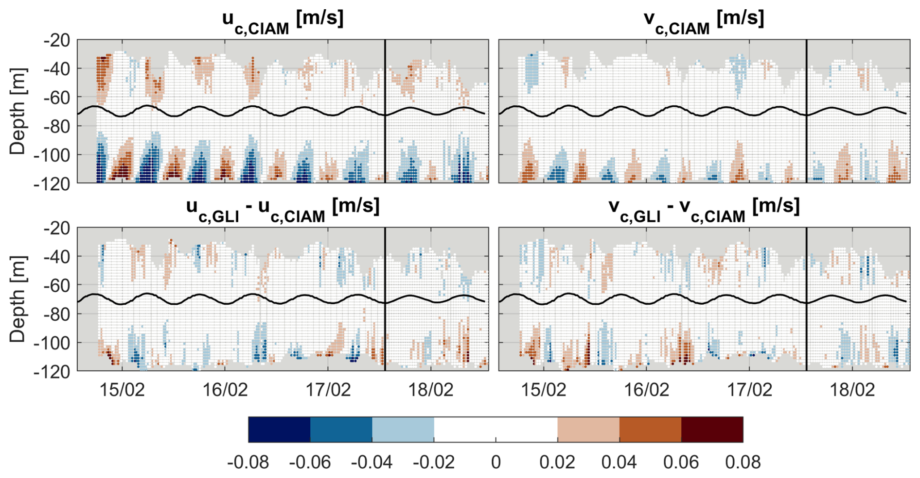
Figure 9 Up) Components of the residual currents (deviation from the depth-averaged constant) measured by the CIAM moored-ADCP. Down) Components of the difference between the residual currents measured by the glider-AD2CP and CIAM moored-ADCP. Residual currents are defined as $u(z,t)-\stackrel{\mathrm{‾}}{u}\left(t\right)$, where $\stackrel{\mathrm{‾}}{u}\left(t\right)$ is the depth-averaged velocity computed from Eq. (2). The black undulated line represents the free surface variation with tide (put in the middle of the graphic for a better display), computed from the GV1 pressure sensor. The black straight line delineates the BU and VM survey periods.

Near-bed discrepancies could in principle be linked to internal waves, which are known to generate baroclinic motions and shear layers close to the seabed in stratified conditions (Moum et al., 2007; Green et al., 2008). Although such motions cannot be entirely excluded, the vertical homogeneity of the water column makes their sustained generation and propagation unlikely. Indeed the glider's CTD data (not shown) measured maximum differences of 0.02 °C and 0.01 PSU in the vertical profiles of temperature and salinity respectively, in the whole water column and during all the survey period. Then the observed vertical patterns of currents are more readily explained by frictionally driven vertical shear within the bottom boundary layer. This process was not expected to spatially vary significantly within the boundary of the campaign area, which was confirmed by validation metrics. Its thickness, estimated between 9–14 m from the Soulsby (1983) formulation using near-bed tidal current amplitudes and the local tidal frequency, decreases over the glider mission in phase with the weakening of the depth-averaged current (from ∼0.3 to ∼0.2 m s⁻¹ on average, Fig. 8). This relationship supports the interpretation that bottom boundary layer thickness is primarily controlled by near-bed stress and dissipation associated with bottom friction (Soulsby, 1983). Within this frictional layer, tidal velocities decay sharply toward the seabed over meter-scale distances, creating strong vertical gradients that are challenging to resolve with glider measurements. As shown by Gentil et al. (2022), the vehicle's coarser vertical sampling and reduced bin overlap near the seabed can hinder accurate reconstruction of such steep profiles. Consequently, even modest differences of only ∼2 cm s⁻¹ between glider and mooring measurements may correspond to substantial limitations in capturing the fine-scale dynamics of the near-bed flow.

5.2 SPMC Estimates

Section 5.2.3 gives a description of the spatio-temporal dynamics of the turbidity observed by the glider. But, first, Sect. 5.2.1 compares the optical sensors and Sect. 5.2.2 compares the optical and acoustic sensing of turbidity in terms of Suspended Particulate Matter Concentration (SPMC).

5.2.1 Optical sensors comparison

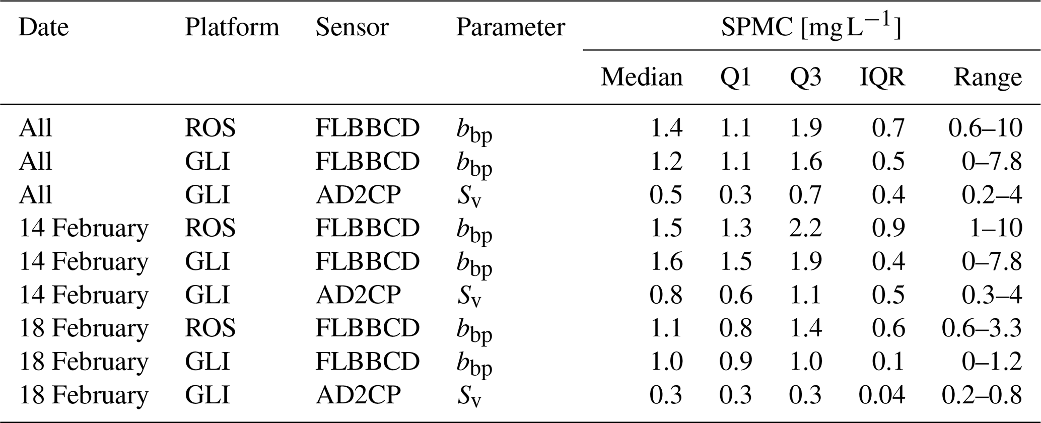
In assessing SPMC, the main sensor to put on board a glider is a turbidimeter (Maa et al., 1992), provided that its output units, either in FNU, NTU or in m⁻¹, is well converted to mg L⁻¹ according to a proper in situ calibration. Here, as a posteriori checks, Table 5 provides statistics for SPMC values measured using the two FLBBCD sensors: one onboard the CTD-Rosette and the other onboard the glider. These statistics show fairly consistent SPMC ranges between the two sensors, especially for the median values, even though the interquartile range (IQR) shows that the CTD-Rosette profiles appear to be a bit more widely spread. These results show at least that, despite their laboratory calibrations performed at 6 years intervals (see Sect. 4.8), both optical sensors seem to broadly record consistent ranges each other.

Table 5 Statistics of SPMC values derived from optical and acoustic sensors. The optical backscattering coefficients are measured by both the CTD-Rosette (ROS) and the glider (GLI), and the acoustic backscattering coefficient is measured by the glider (GLI). Statistics are given for the whole survey period (All) and for the days of 14 and 18 February 2021. Q1 is the first quartile, Q3 is the third quartile, IQR is the Inter-Quartile Range. The extremum Range is [min–max].

5.2.2 Acoustic SPMC estimation

Optical turbidimeters are not always well correlated to SPMC (Downing, 2006). A more comprehensive observation of SPM can make use of both optical and acoustic sensors (Fettweis et al., 2019; Haalboom et al., 2021). Here, Table 5 provides statistics for both optical and acoustic SPMC (with the AD2CP onboard the glider). From these statistics, we see that acoustic SPMC values are broadly lower than the optical ones by roughly a factor two. Indeed, it appears that the calibration between the optics and the acoustics, done in Sect. 4.9, deviates from a linear relation at low and high SPMC values (see Fig. 5) which can explain this factor two.

5.2.3 Temporal and vertical dynamics

Figure 10 displays the temporal evolution of SPMC simultaneously recorded by the glider in three vertical layers: Deep [−125 m; −100 m], Middle [−100 m; −60 m] and Surface [−60 m; −20 m]. Since the acoustic and optical backscattering coefficients derived from the AD2CP and FLBBCD sensors are correlated (see Fig. 5), both acoustic and optical-derived SPMC show similar patterns. However, some differences are observed, with the optical sensor recording higher SPMC near the seafloor compared to the acoustic sensor. This discrepancy suggests that the bottom layer is primarily composed of fine particles, which are more effectively detected by the optical sensor than by the acoustic one.

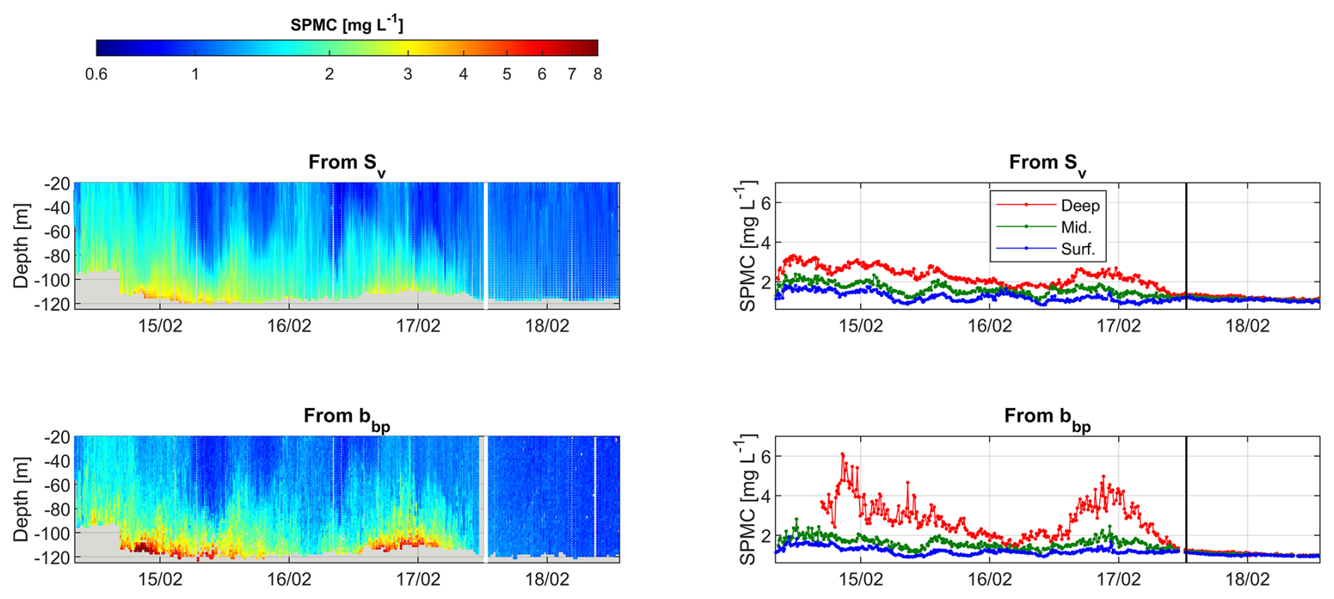
Figure 10 SPM concentrations recorded by the glider. Top: SPMC from acoustic backscattering (S_v). Bottom: SPMC from optical backscattering (b_bp). On the left are hovmöller diagrams. On the right are solid lines displaying corresponding levels in the three main water column layers defined by the following depth ranges: Deep = [−125; −100], Mid. = [−100; −60] and Surf. = [−60; −20] m. Vertical lines separate BU (Butterfly) and VM (Virtual Mooring) periods: white lines on the left and black lines on the right.

In terms of temporal evolution, the glider observes a higher vertical SPMC dynamics during the BU period than during the VM period. In fact, over this period the glider is moving from muddy to sandy to gravel bottoms and the VM phase is on gravel as tides get smaller. This could be a reason why the turbidity is much lower (regardless of the acoustic vs. optical calibration law). In particular two intense events appear in the BU period. They are centered around 17:00 UTC 14 February, and around 00:00 UTC 17 February. During these first and second events, optical values of SPMC in the deep layer are up to 7.8 and 5 mg L⁻¹, respectively, indicating the presence of a well-developed bottom nepheloid layer with a thickness of 15–20 m (Fig. 10). In the intermediate and surface layers both acoustic and optical SPMC are consistent and give values mostly comprised between 1–2 mg L⁻¹. Finally, during the VM period, SPMC levels drop (either from acoustics or optics) with values below 1.5 mg L⁻¹.

In summary, the glider successfully captures the temporal and vertical dynamics of SPMC, with some consistency between optical and acoustic measurements. Additionally the glider demonstrated its capability to provide high-resolution measurements of both barotropic and baroclinic currents with high consistency across platforms. Together, these findings confirm the glider's suitability as a platform for observing hydro-sedimentary processes in coastal zones, providing a solid foundation for process-oriented studies, and allow to compute fluxes.

5.3 SPM: linking properties and transport in a tidal shelf environment

In addition to SPMC range, information on the Particle Size Distribution (given in Sect. 5.3.1) is decisive in the study of hydrosedimentary processes that contribute to suspended sediment fluxes observed and presented in Sect. 5.3.2.

5.3.1 Particle size distribution (PSD)

At each vertical bin of the CTD-Rosette profiles, the LISST-100X measured C_v [µL L⁻¹]: the volumetric concentration by size classes of particles. The PSD is analysed over 30 size classes, logarithmically distributed between 2.4 and 296 µm (center of classes). Table 6 gives the statistical values of C_v, and as well as for the total volumetric concentrations: C_v,Tot [µL L⁻¹]. Median concentration values acquired on 14 February are globally twice as those acquired on 18 February, although concentrations show higher maximal values that day. The median diameter d₅₀ keeps a typical value round 35 µm, with only a slight decrease from 14 to 18 February. Throughout the water column, PSDs are globally homogeneous, except in the upper part (heights above 70 m) on 18 February where a population of particles coarser than the main mode gradually appears, its median size growing as the sea surface approaches (not shown) and could correspond to plankton.

Table 6 Statistical parameters obtained from the LISST measurements onboard the CTD-Rosette stations deployed within the full water column on 14 February and 18 February 2021: with size classes volumetric concentrations C_v, total volumetric concentrations C_v,Tot, and median diameter d₅₀.

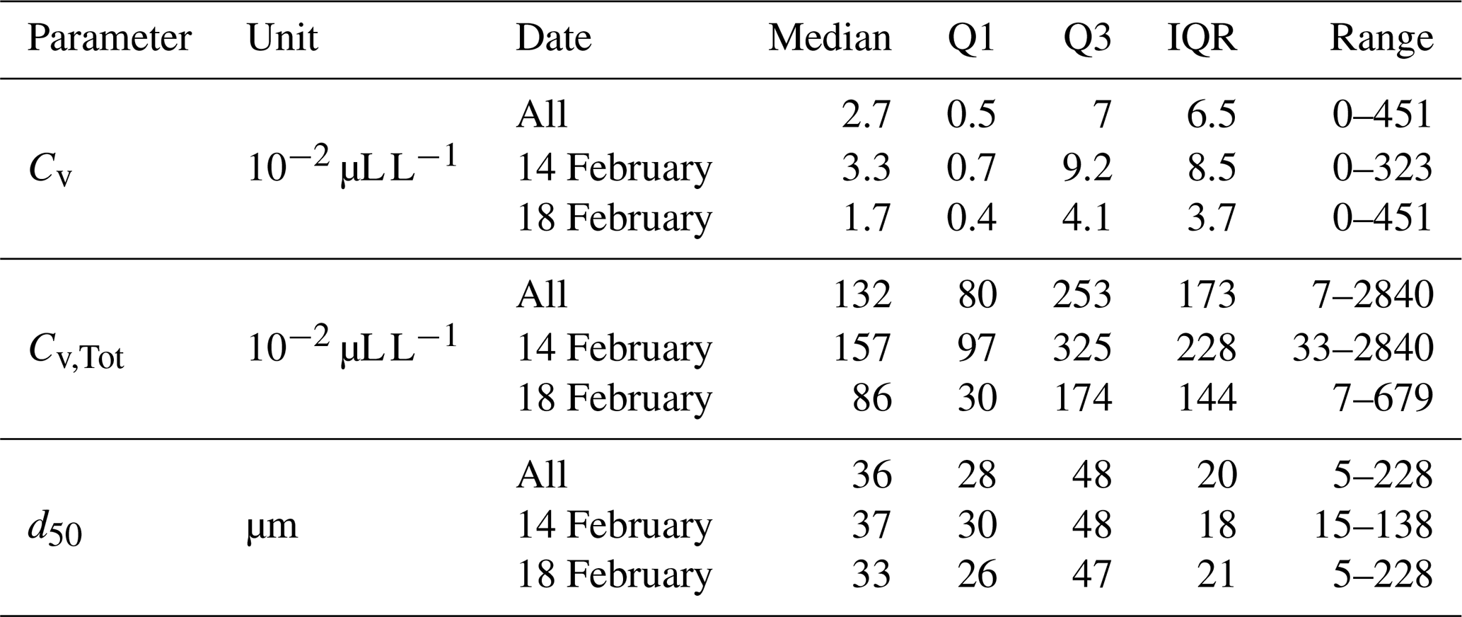
Figure 11 (right panels) displays the Median Particle Size Distribution (PSD) from the 3 m above seabed, in terms of volumetric normalized concentrations C_v,norm (C_v divided by C_v,Tot), along with the turbidity measurements of the CTD-Rosette turbidimeter. The main mode around 35 µm can be well seen on PSD curves, but a second mode, around 5 µm also appears. This second mode is only slightly distinguishable on 14 February but stands out clearly on 18 February. It corresponds to a turbid background of very fine grain size sediments superimposed on the main turbidity signal. On 18 February the level of the main turbidity signal decreases (Fig. 11d, left panels), with a lesser contribution of the main mode at 35 µm, which highlights the second mode at 5 µm. The origin of this second mode remains unknown. It could eventually be flocculi, although flocculi should have typical sizes between 10–20 µm (Lee et al., 2012).

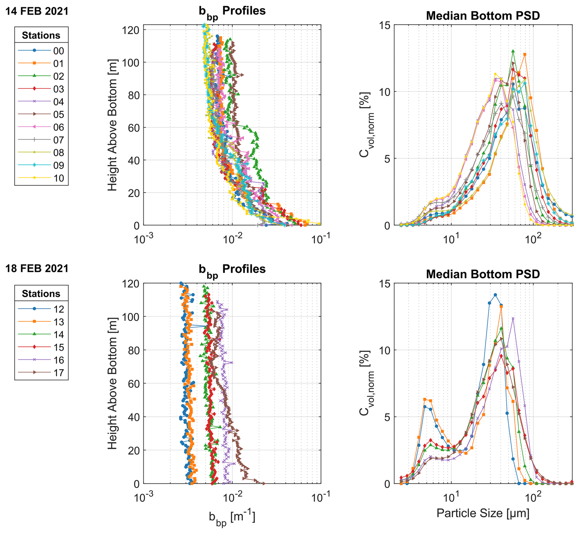
Figure 11 SPM measurements from the CTD-Rosette profiles recorded on 14 February 2021 (upper panels) and on 18 February 2021 (lower panels) stations. On the left are Optical backscattering coefficients (b_bp) recorded with the FLBBCD triplet. On the right are Median Bottom Particle Size Distribution (PSD) recorded with the LISST-100X and expressed in terms of normalized volumetric concentrations C_v,norm. The median was calculated from data collected within 3 m of the seabed.

5.3.2 Derived SPM fluxes

Estimation of SPM fluxes is still poorly documented at the scale of entire continental shelves. There are almost exclusively single point measurements from bottom tripods, buoys and moorings (Guillén et al., 2006) describing the impact of extreme events at high temporal resolution. Few studies using gliders investigated the sediment transport at the scale of continental shelves (Gentil et al., 2020, 2022; Miles et al., 2015). Thanks to the installation of both a turbidimeter and an AD2CP onboard a glider, such platform is able to assess fluxes, in particular the integrated flux, here notated Q_S. Figure 12 demonstrates this capacity. The figure shows that the observed instantaneous flux obviously varies with the tide: fluxes vary from zero to nearly 40 $\mathrm{g}{\mathrm{m}}^{-\mathrm{1}}{\mathrm{s}}^{-\mathrm{1}}$ in the direction of the tidal ellipse. The black and blue curves show that fluxes derived from the acoustics often underestimate those derived from the optics by around 30 % (because it underestimates SPMC at higher concentrations). Then an AD2CP alone onboard a glider could provide an acceptable order of magnitude of such fluxes. However this must require an appropriate calibration of the AD2CP in terms of SPMC with concomitant SPM filter acquisitions, which is not an obvious task with a moving glider. Here we provided turbidimeters measurements using the same optical model onboard both the glider and our CTD-Rosette deployed in the same area, which allows us to provide an effective calibration (by successive deduction) of both the optical and acoustic sensors onboard the glider. Hence, both a turbidimeter and an AD2CP is certainly mandatory for such flux observation by glider.

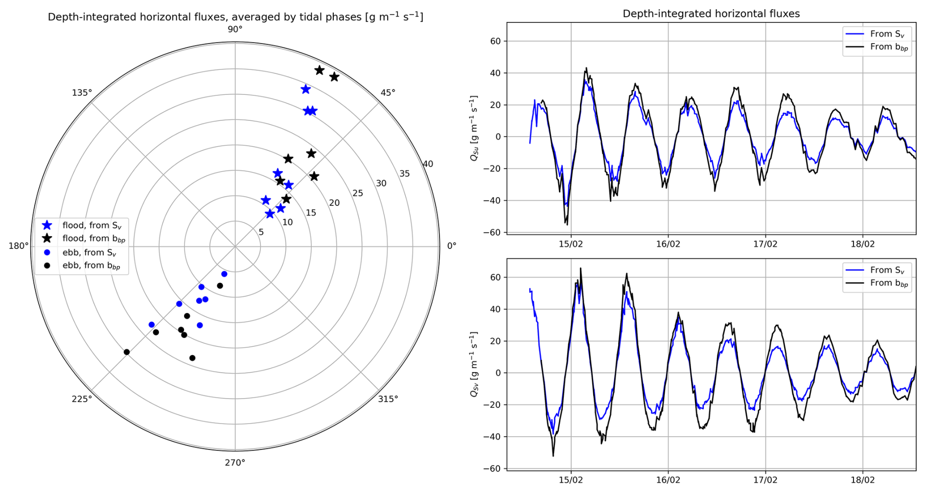
Figure 12 Depths-integrated SPMC fluxes derived from the glider currents and concentrations measured either with its AD2CP (S_v) or with its FLBBCD sensor (b_bp). Left: directions and amplitudes of averaged fluxes during full periods of floods (stars) and ebbs (dots); Right: time series of the instantaneous fluxes (following the tide mainly). NB: data for b_bp starts later due to the missing near bottom data for the first half-day of the campaign.

To have an idea of the resulting suspended sediment transport in a given direction, residual fluxes are preferable to instantaneous fluxes (the latter being subject to the ebb and flow of the tides). To assess residual fluxes we decided here to apply a basic tidal filter on the observed instantaneous fluxes from the glider. This filter is a two-pass running average filter using 25 and 13 h windows, applied to both components U and V of the instantaneous fluxes: the first 25 h window removes most of the tidal signal, and the 13 h window removes some remaining semidiunal signals (Shirahata et al., 2016). Applying such a filter here assumes the fluxes observed by the glider in the whole area are fully consistent in space. This is certainly the case for the barotropic currents, as demonstrated by the high correlation between currents observed by the two moorings GV1 and CIAM, but is not demonstrated in terms of SPMC. Figure 13 shows orders of magnitudes round 1 $\mathrm{g}{\mathrm{m}}^{-\mathrm{1}}{\mathrm{s}}^{-\mathrm{1}}$ heading mainly north that are consistent with those modelled for winter conditions in the area of the “Grande Vasière” by Mengual et al. (2019).

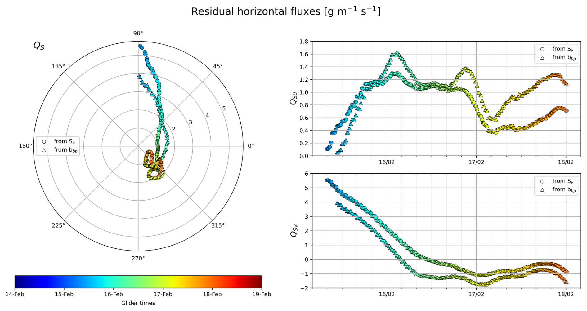
Figure 13 Same as Fig. 12 except for residual fluxes (after the tidal signal has been removed).

Accuracy of suspended sediment fluxes estimates depends on both precision of ocean current measurements and SPMC. If we define a parameter called “flux magnitude”, notated M_Q, with its two components u and v calculated separately as follows:

$$\begin{array}{}\text{(14)}& {\displaystyle }{\displaystyle }{M}_{Qu}(t,z)={\log }_{\mathrm{10}}\left(\text{SPMC}\right(t,z\left)\right)\cdot u(t,z)\end{array}$$

Then its typical error measured by the glider, in terms of RMSD, can be estimated as follows (for its two components u and v):

$$\begin{array}{}\text{(15)}& {\displaystyle }{\displaystyle }\text{RMSD}\left(M_Q\right)=\text{RMSLD}\left(\text{SPMC}\right)\cdot \text{RMSD}\left(u\text{or}v\right)\end{array}$$

This formula is valid because error biases are small compared to their respective RMSD values. Also this formula assumes that SPMC and (u or v) are two independent random variables. Then, applying this equation, we take the RMSLD value from Eq. (11) and a mean RMSD value of round 3 cm s⁻¹ for the currents (from Table 3). Then we obtain the following average error estimation for the 'flux magnitude':

$$\begin{array}{}\text{(16)}& \begin{array}{rl}\text{RMSD}\left(M_Q\right)& =\mathrm{0.11}\times \mathrm{3.0}\\ & =\mathrm{0.33}{\log }_{\mathrm{10}}\left(\mathrm{mg}{\mathrm{L}}^{-\mathrm{1}}\right)\mathrm{cm}{\mathrm{s}}^{-\mathrm{1}}\end{array}\end{array}$$

Because SPMC error distribution is lognormal and (u,v) error distributions are normal, this unique value of 0.33, on its own, fully describes the error distribution of the “flux magnitude”, and so, by deduction, describes the error distribution of the flux of SPM Q_F. However, the range and associated unit of this value are not easy to interpret.

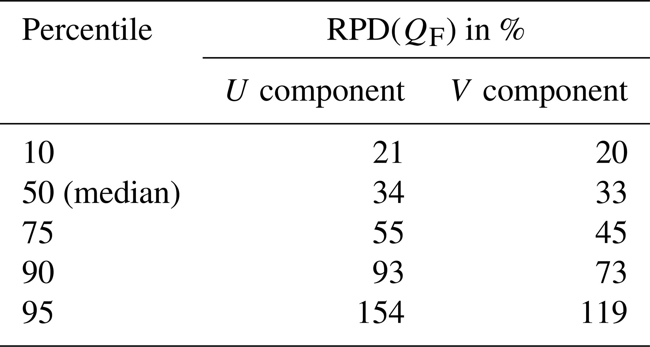
Instead, one may prefer to have a broad idea of the flux errors in terms of relative percent difference (RPD). For that purpose, we calculated the relative percent errors for the fluxes recorded at all comparison cells between CIAM and GLI. To do that, we simply added (because the RPD of the product of independent random variables is the sum of each RPD value) the value of RPD(SPMC), that is 17 %, to all relative percent differences recorded for the currents. Table 7 gives the percentiles of the statistical distribution obtained. Large errors (for percentiles 90 and 95 for instance) correspond to low absolute currents much smaller that 3 cm s⁻¹, that cannot be correctly observed with a typical error of 3 cm s⁻¹. Nonetheless, the median RPD has a value round 33 % which appears acceptable compared to the values ranging from 20 % to 600 % estimated in Gentil et al. (2020).

Table 7 Percentiles of the statistical distribution of the Relative Percent Difference (RPD) of the instantaneous error flux Q_F based on the difference of the currents recorded between CIAM and GLI.

The advantage of using gliders is to increase resolution measurements at both spatial and temporal scales and investigate extreme events such as floods and storms. Joined use of glider data and their assimilation in modeling work then strongly increase our interpretation of sediment transport on continental shelves (Estournel et al., 2023). Accuracy of suspended sediment fluxes estimates depends on both precision of ocean current measurements and SPMC. While the accuracy of ocean currents is relatively well constrained, the greatest error comes from SPMC estimation. Both acoustic and optical sensors are widely used but strongly depend on particle size, nature and concentration (Many et al., 2016).

From previous works, the main processes involved in sediment transport on continental shelves are of two origins: anthropogenic ones such as bottom trawling (Palanques et al., 2006), installation of offshore wind farms (Vanhellemont and Ruddick, 2014) and natural ones: with floods and storms. While suspended sediment transport estimates outside extreme events remain lower by typically one order of magnitude (Gentil et al., 2020), glider deployments can help estimate sediment transport during these extreme events.

However, analysis of glider data often occurs after the recovery of the instruments at sea a few times later. Using gliders and transmitting data in real time can also have advantages in investigating impacts of human activities on continental shelves. Real-time data could also help managers and decision-makers of a regional area in the evaluation of environmental changes that might affect coastal ecosystem such as marine heat waves, algal blooms, or pollutant dispersion.

6 Conclusions

The present study deals with the validation of tidal current, acoustic backscatter, and optical turbidity measurements acquired from the SeaExplorer underwater glider (ALSEAMAR), equipped with a Nortek-AD2CP profiler and Seabird-FLBBCD triplet. Glider-based measurements were acquired during five days in February 2021 in the Bay of Biscay (Atlantic continental shelf) under typical winter conditions. Measurements were successfully validated by comparison with in situ profile data simultaneously acquired nearby from two moored ADCPs, and with optical turbidity and a LISST mounted on CTD-Rosette sampler. The main conclusions of this study are:

1. The AD2CP-SeaExplorer glider system is a suitable platform to monitor the water column-resolute ocean currents over the continental shelf in mesotidal settings. RMSD is in the order of O(3 cm s⁻¹), of the order of the combined measurement uncertainty on the glider and mooring data.

2. In winter conditions, AD2CP-derived acoustic backscatters yield a satisfactory description of the sediment concentration in the nepheloid layer. In combination with optical turbidity, insights on the sediment distribution are also obtainable.

3. In situ calibration of glider-based backscatter sensors with gravimetric measurements will make it possible to accurately estimate suspended particle fluxes at high spatio-temporal scales over the shelf, but this requires a rosette sampler in the vicinity or a similar water-sampling device onboard the glider.

4. During our investigation period, we could not only observe bottom nepheloid layers (with typical concentrations of several mg L⁻¹) but also residual fluxes, that show orders of magnitudes and directions consistent with those modelled for winter conditions in the area (round 1 $\mathrm{g}{\mathrm{m}}^{-\mathrm{1}}{\mathrm{s}}^{-\mathrm{1}}$ heading mainly north).

In conclusion, this work provides a promising technological breakthrough for the fine-scale monitoring of ocean water quality and the outcome of associated suspended matter, for which real-time information on currents and fluxes can also be crucial.

Appendix A: Abbreviations

The following abbreviations are used in this manuscript:

ADCP	Acoustic Doppler Current Profiler
bbp	optical backscattering coefficients, derived
	from the dedicated sensors
BU	Butterfly-patterned mobile survey period
	(realized by the SeaExplorer glider)
CU	Combined measurement Uncertainty
DAC	Dive Averaged Current
IQR	Interquartile Range, such as IQR = Q3–Q1
LADCP	Lowered ADCP
LAT	Lowest Astronomical Tide (chart datum)
mab	meters above bottom
PSD	Particle Size Distribution
Q1	First quartile
Q3	Third quartile
SPM	Suspended Particulate Matter
SMPC	Suspended Particulate Matter Concentration
STD	Standard Deviation
Sv	acoustic backscatter, derived from the
	glider-AD2CP measurements
VM	Virtual Mooring survey period (realized by
	the SeaExplorer glider)