Forcing-dependent submesoscale variability and subduction in a coastal sea area (Gulf of Finland, Baltic Sea)

Submesoscale (SMS) processes in a stratified coastal environment of the Gulf of Finland (Baltic Sea) were investigated using glider missions and a realistic simulation with a grid spacing of 0.125 nautical miles. The study period covered the transition from developing to established seasonal stratification. SMS variability, defined as small-scale anomalies of temperature and salinity cancelling each other's contribution to density (spice), was concentrated around the base of the upper mixed layer (UML) in spring and within the seasonal thermocline in late summer. We suggest that this shift was caused by the changes in surface heat flux and wind forcing. Both observations and simulations revealed events of high SMS variability, which can be related to background mesoscale dynamics and changes in wind forcing. We examined the event in which elevated spice in the subsurface layer did not coincide with the high Rossby number O(1) in the surface layer but instead appeared offshore of a coastal baroclinic current. Sloping isopycnals and intensified vertical velocities pointed to active SMS subduction. We propose that frontal instabilities, likely related to flow–topography interactions, drive the lateral and downward transport of surface waters, contributing to tracer redistribution below the thermocline.

1 Introduction

Submesoscale (SMS) flows, occupying the intermediate horizontal scale of ∼1 km (Taylor and Thompson, 2023), are increasingly recognized as critical drivers of vertical exchanges of heat, carbon, and nutrients in the upper ocean, with important implications for stratification, biogeochemical cycling, and ecosystem productivity (e.g., Mahadevan, 2016). These processes bridge the energy transfer between larger, geostrophically balanced motions and microscale turbulence, making them central to upper-ocean dynamics (Capet et al., 2008; Naveira Garabato et al., 2022).

The ocean is a vast dynamic system driven by winds, tides, and density gradients due to temperature and salinity differences. These forces generate motion across a wide range of spatial scales, from large-scale geostrophic currents to small-scale turbulent mixing. Traditionally, upper ocean turbulence has been understood as a combination of mesoscale quasi-geostrophic eddies, internal waves, and microscale three-dimensional turbulence. Mesoscale dynamics, with characteristic horizontal scales of O(10–100) km in the ocean and O(5–20) km in the Baltic Sea, are characterized by small Rossby number ($Ro=\frac{U}{fL}$, Ro≪1) and large Richardson number ($Ri=\frac{N^{\mathrm{2}}{H}^{\mathrm{2}}}{U^{\mathrm{2}}}$, Ri≫1), reflecting dominance of rotational and buoyancy forces (Taylor and Thompson, 2023). Here, U is a characteristic horizontal velocity scale, L and H are horizontal and vertical length scales, f is the Coriolis parameter, and N is the Brunt–Väisälä frequency. In contrast, SMS dynamics are characterized by Ro O(1) and Ri<1, indicating a dynamic regime where rotation, stratification, and inertial forces all play important roles (Thomas et al., 2008). The weaker rotational constraint allows SMS processes to generate strong vertical velocities (e.g., Chrysagi et al., 2021; Tarry et al., 2022).

Recent advances in observational technology, particularly the use autonomous gliders, have significantly improved our ability to detect SMS structures. With their high spatial resolution and adaptive sampling capabilities, gliders are well suited to capturing the smaller-scale variability associated with SMS processes. For example, Jhugroo et al. (2020) identified low-salinity SMS features driven by riverine input in a New Zealand shelf sea, which could intensify local stratification and displace a well-mixed surface layer up to 100 km offshore before being entrained by regional currents. Similarly, Bosse et al. (2021) used gliders to sample frontal zones in the northwestern Mediterranean Sea, revealing strong vertical motions and subduction events. In the Baltic Sea, studies such as by Carpenter et al. (2020) and Salm et al. (2023) have begun to reveal the role of SMS dynamics in shaping water column structure and vertical exchanges. However, given the region's complex stratification and ecological sensitivity, further glider-based studies are needed to resolve SMS processes and their biogeochemical implications in more detail.

This study focuses on the Gulf of Finland (GoF), an elongated sub-basin of the Baltic Sea – a semi-enclosed, brackish, shallow marginal sea in Northern Europe that stretches from 54 to 66° N. The sea has limited water exchange with the North Sea, and the input of fresh river water is large. The Neva River, the largest freshwater source, discharges at the eastern end of the GoF. Meanwhile, saltier water is transported into the gulf through its western border, creating a pronounced horizontal salinity gradient across the gulf.

The flow field in the GoF, which governs the freshwater transport and shapes both horizontal and vertical salinity gradients, is significantly influenced by the wind (Lilover et al., 2017; Westerlund et al., 2019). Prevailing along-gulf winds can establish a wind-driven circulation pattern, with currents along the wind near the coasts and counter-flows in the central gulf (Lips et al., 2017; Elken et al., 2011). These circulation patterns enhance transverse salinity gradients. Along-gulf winds also promote upwelling and downwelling events along the northern and southern coasts (Kikas and Lips, 2016; Lehmann et al., 2012). The summer upwelling events are typically associated with substantial temperature gradients at the sea surface (Lips et al., 2009; Uiboupin and Laanemets, 2009), and due to the strong horizontal and vertical salinity gradients and the development of jet currents along the upwelling fronts, also lead to pronounced salinity redistribution (Suursaar and Aps, 2007). Frontal structures and hydrographic variability associated with coastal upwelling serve as indicators of enhanced vertical mixing (Lips et al., 2009) and the emergence of SMS features, such as filaments and eddies (Väli et al., 2017).

During spring and summer, a seasonal thermocline typically forms at depths of 10–30 m. Beneath this layer – and throughout the water column during the remainder of the year – vertical stratification is predominantly controlled by salinity. The quasi-permanent halocline lies below 60 m on average (Liblik and Lips, 2017). In winter and early spring, shallow haline stratification can also develop because of freshwater advection (Liblik et al., 2020; Lips et al., 2017). In the GoF, the vertical salinity gradient has an equally important role alongside temperature in shaping the density stratification of the water column, highlighting a key difference from general open ocean conditions.

Building on previous observational evidence of SMS features in the GoF (Salm et al., 2023), this study aims to further investigate the role of SMS processes in this stratified coastal environment using a combination of observational and numerical tools. The appearance of SMS features associated with the development of a mesoscale front and changing wind forcing was documented based on mission data from spring 2018 (Salm et al., 2023). Here, we extend the analysis to all three missions conducted in the same area in spring–summer 2018–2019.

We examine tracer variability, specifically spice, which represents temperature and salinity variations that compensate for each other in density (Rudnick and Cole, 2011). We propose that scale-specific spice at horizontal scales of a few kilometers can be used as an indicator of SMS activity, especially in conditions when temperature and salinity contribute comparably to density stratification. In the GoF, this is applicable in late spring and summer, when both thermal and haline stratification are significant. Although spice can potentially be advected over some distance, the rapidly changing, wind-driven circulation in the GoF (Lilover et al., 2017) limits the transport of SMS features, thereby justifying a localized analysis. Ultimately, spice reveals anomalies and spatial gradients along isopycnals, where SMS processes often act. It serves as a proxy for SMS intensity capturing variability without being masked by vertical excursions of isopycnal surfaces, i.e., internal waves.

We focus on the upper half of the water column, where SMS activity is most prominent and glider data are more densely sampled, allowing more robust analysis. Our study is limited to the spring–summer period, when seasonal stratification develops and becomes well established. This time window allows us to focus on our main objective of understanding SMS generation under stratified conditions.

To complement and expand upon glider observations, we employ a high-resolution numerical model with SMS-permitting horizontal grid spacing (∼232 m), enabling us to characterize the dynamical background and infer SMS activity beyond the limited scope of in situ measurements. For meaningful SMS analysis, model data were averaged over a 10×10 km study window (“time series box”; 59.67–59.76° N, 25.06–25.25° E; see Fig. 1). This averaging accounts for the potential spatial and temporal displacement of SMS features, which are highly sensitive to small changes in initial conditions, model resolution, and parameterized processes. By situating glider observations within a wider model domain, the analysis accommodates these discrepancies and captures how background mesoscale conditions modulate SMS activity, thus enabling more robust interpretations of physical variability.

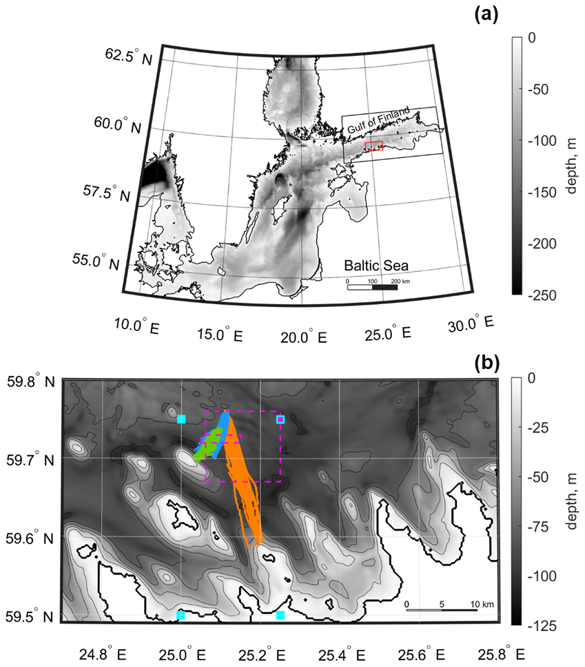
Figure 1 Map of (a) the Baltic Sea and (b) the study area. The red rectangle in panel (a) indicates the location of the study area shown in panel (b). Depth isolines in panel (b) are shown with a step of 20 m. Glider missions from May–June 2018, May–June 2019, and July–August 2019 are shown in orange, blue, and green, respectively. The larger magenta box marks the “time series box” chosen for the modelled data, while the smaller magenta box indicates the area common to all missions (59.72–59.73° N 25.05–25.15° E), used for comparing glider and model data. The positions of ERA5 grid points used for extracting radiation data are shown by cyan squares and wind data by the magenta square. The colormap shows the bathymetry used in the model.

The following hypotheses are considered in this study. First, we suggest that SMS variability is modulated by both atmospheric forcing, particularly surface heat flux and wind stress, and the background (larger-scale) hydrographic structures, including mesoscale frontal gradients. Second, we propose that topographically or forcing-induced instabilities of baroclinic coastal currents create favourable conditions for SMS subduction, enabling offshore and downward transport of tracers. To test these hypotheses, we use glider data and high-resolution simulations to characterize temporal, vertical and horizontal distributions of SMS features and explore associated dynamical forcing. These complementary approaches allow us to link observed variability at the submesoscale with the underlying physical mechanisms and evaluate the role of SMS processes in stratified coastal environments.

The paper is organized as follows: Sect. 2 introduces the observational datasets, the numerical experiment, and the analysis methods; Sect. 3 presents the results, focusing on the spice variability and the SMS-permitting events; Sect. 4 discusses the implications of our findings for SMS activity in coastal stratified seas; Sect. 5 concludes with a summary of key results and their broader relevance.

2 Data and methods

2.1 Glider observations

Although originally conducted for different research objectives, three glider missions in the GoF, Baltic Sea (Fig. 1), collectively provide a dataset for this study. The field campaigns took place from 9 May to 6 June 2018, from 21 May to 19 June 2019, and from 21 July to 10 August 2019, during which an autonomous underwater vehicle, the Slocum G2 Glider MIA, collected oceanographic data along predefined transects. In May–June 2018, an 18 km long transect was sampled 26 times, and in 2019, 4.5 and 5.5 km transects were each sampled over 90 times. In total, over 12 000 profiles were gathered. These transects were oriented across the southern coast of the GoF, capturing cross-shore variability. The glider profiled the water column from the surface down to depths of 80–100 m, depending on the position. While under the surface, the glider started to turn around either 4 m before the surface or 5–6 m before the seafloor. Raw data were quality controlled following procedures adapted from Argo quality control protocols (Wong et al., 2025). Corrections for sensor response time and thermal lag were applied to minimize differences between two consecutive CTD profiles, following the approach described by Salm et al. (2023). Up- and downcasts were bin-averaged to a uniform 0.5 dbar vertical grid and arranged as profiles. For the analysis, the data fields were interpolated onto a regular grid with a time step of 10 min, corresponding to an average horizontal distance of 130 m.

2.2 Model setup

We used a three-dimensional nested setup of the General Estuarine Transport Model (GETM; Burchard and Bolding, 2002) to simulate the circulation and the temperature and salinity distributions in the GoF. GETM is a primitive-equation, free-surface, hydrostatic model with built-in vertically adaptive coordinates (Gräwe et al., 2015; Hofmeister et al., 2010; Klingbeil et al., 2018). Such a grid is a generalization of sigma layers with the potential to enhance vertical resolution near boundaries and in layers with strong stratification and shear (Klingbeil et al., 2018). Previous studies have shown that the total variation diminishing (TVD) advection scheme, combined with the superbee limiter, reduces numerical mixing in simulations (Gräwe et al., 2015). Vertical mixing in the GETM was calculated by coupling it with the General Ocean Turbulence Model (GOTM; Umlauf and Burchard, 2005). More precisely, the two-equation k–ε turbulence model (Burchard and Bolding, 2001; Canuto et al., 2001) was used in the simulation.

The entire GoF was the high-resolution model domain, with a uniform horizontal grid spacing of 0.125 nautical miles (approximately 232 m) and 60 adaptive layers in the vertical. Original bathymetry was obtained from the EMODnet database (http://summary.emodnet-hydrography.eu/data-products, last access: 1 June 2025) with a resolution of $\mathrm{1}/\mathrm{16}$ arcmin (approximately 150 m). Bathymetry data were averaged to the model resolution, and missing values were interpolated using the nearest neighbour (NN) technique.

The high-resolution simulation with an open western boundary at the GoF entrance was performed starting on 3 December 2017. The initial temperature and salinity fields and boundary conditions were taken from coarse-resolution simulations covering, respectively, the entire Baltic Sea with a grid step of 1 nautical mile (see Väli et al., 2024 for more details) and the Baltic Proper (including the GoF) with a grid step of 0.5 nautical miles (see Zhurbas et al., 2018 and Liblik et al., 2020, 2022 for more details). As all setups use adaptive coordinates, we first interpolated the profiles from the coarse-resolution model to a fixed 5 m vertical resolution before spatial interpolation to the high-resolution model grid using the NN method. If needed, the profiles were extended to the bottom of the high-resolution grid to compensate for the bathymetric differences. The model run started from a motionless state with zero sea surface height and current components. Previous studies by Krauss and Brügge (1991) and Lips et al. (2016b) have shown that the spin-up time for the Baltic Sea model under atmospheric forcing is less than 10 d. For the boundary conditions, the temperature, salinity, and current profiles, as well as sea surface height, all with a 1 h temporal resolution from the 0.5 nautical mile resolution simulation, were used. The same model setup was used by Siht et al. (2025), where further details and validation results are presented. Some quantitative information on model performance regarding stratification and SMS variability, which are the focus of the present paper, are given in Sect. 3.1.

The atmospheric forcing at the sea surface (the momentum and heat flux) was calculated from the European Centre for Medium-Range Weather Forecasts atmospheric reanalysis dataset (ERA5, Hersbach et al., 2020) by utilizing wind components and other relevant parameters (air temperature, total cloudiness, relative humidity, sea level pressure) for bulk formulae by Kondo (1975). All meteorological parameters were interpolated bi-linearly to the model grid. The riverine freshwater input to the Baltic Sea was taken from the dataset produced for the Baltic Model Intercomparison Project (BMIP; Gröger et al., 2022) based on the E-HYPE (Lindström et al., 2010) hindcast and forecast products by Väli et al. (2019). There were 91 rivers in the dataset, of which 13 were in the GoF.

2.3 Submesoscale analysis

While air-sea fluxes, turbulent mixing, and advection introduce variability in the seawater properties, the dynamical processes act quickly to remove density differences. Spice – the combination of temperature and salinity variations that cancel each other's contribution to density – is the residual signal that remains (Rudnick and Ferrari, 1999). Spice was defined as the sum of the temperature anomalies, ΔT, scaled by the thermal expansion coefficient, α, and the salinity anomalies, ΔS, scaled by the haline contraction coefficient, β, as shown in Eq. (1):

$$\begin{array}{}\text{(1)}& \mathrm{spice}=\mathit{\alpha }\mathrm{\Delta }T+\mathit{\beta }\mathrm{\Delta }S.\end{array}$$

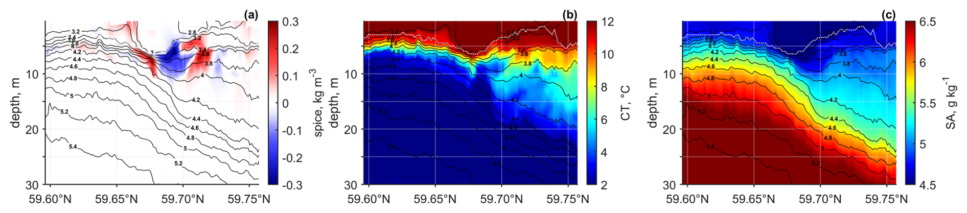
Figure 2 Example sections of (a) spice, (b) temperature, and (c) salinity with overlaid density contours, based on glider data from 24–25 May 2018. The white dashed line indicates the upper mixed layer depth.

The coefficients were calculated according to McDougall and Barker (2011). In this study, anomalies refer to the differences between the measured or modelled Conservative Temperature or Absolute Salinity and their average values along an isopycnal, calculated over a surrounding area of 4 km. For the observations, this was implemented as a moving window along the glider trajectory; for the model, it was computed over a 4×4 km square. The chosen length scale is consistent with the internal Rossby deformation radius in the GoF, which is typically 2–4 km (Alenius et al., 2003). The choice of a 4 km averaging scale offers a practical balance between resolving SMS structures and suppressing high-frequency noise. A smaller averaging scale may exaggerate variability and obscure persistent features, while a larger averaging scale poses a risk of smoothing out key SMS signals. Thus, 4 km averaging preserves the essential gradients and anomalies linked to SMS dynamics without compromising interpretability. Figure 2a shows an example of spice derived from the observations. The patches of positive (negative) spice indicate regions with higher salinities and temperatures (lower salinities and temperatures) compared to the average values in the surrounding 4 km on the same isopycnal surface. Spice effectively highlights smaller-scale (SMS) variability that may be challenging to discern from the vertical sections of temperature and salinity alone (Fig. 2b and c).

The average spice intensity was defined as the root mean square of spice from the sea surface to the depth of minimum temperature. The UML depth was determined as the minimum depth where ${\mathit{\rho }}_z\ge {\mathit{\rho }}_{\mathrm{3}}+\mathrm{0.25}$ kg m⁻³ was satisfied (ρ_z is the density at depth z and ρ₃ at 3 m). The strength and position of the pycnocline, primarily associated with the seasonal thermocline, were analysed based on the maximum squared Brunt–Väisälä frequency (N²) and its corresponding depth. The vertical buoyancy gradient was estimated as N²=b_z, calculated over 2 m vertical intervals. Buoyancy was defined as Eq. (2):

$$\begin{array}{}\text{(2)}& b=-{\displaystyle \frac{g}{{\mathit{\rho }}_{\mathrm{0}}}}\left(\mathit{\rho }-{\mathit{\rho }}_{\mathrm{0}}\right),\end{array}$$

where ρ₀ is the reference density of 1000 kg m⁻³.

Quantities indicative of the SMS regime, such as the Rossby number (Ro), balanced Richardson number (Ri), and horizontal buoyancy gradient, were calculated based on the model data. Ro and Ri were estimated, respectively, as Eq. (3):

$$\begin{array}{}\text{(3)}& Ro={\displaystyle \frac{\mathit{\zeta }}{f}},\end{array}$$

and Eq. (4):

$$\begin{array}{}\text{(4)}& Ri={\displaystyle \frac{f^{\mathrm{2}}{N}^{\mathrm{2}}}{{\left|{\mathrm{\nabla }}_{\mathrm{H}}b\right|}^{\mathrm{2}}}}.\end{array}$$

$\mathit{\zeta }=v_x-u_y$ is the vertical component of relative vorticity, f is the Coriolis frequency, and $\left|{\mathrm{\nabla }}_{\mathrm{H}}b\right|=\sqrt{b_x^{\mathrm{2}}+b_y^{\mathrm{2}}}$ horizontal buoyancy gradient modulus. Centred finite-difference scheme was used to calculate the parameters from the model. Horizontal and vertical steps for estimating gradients were 500 and 2 m, respectively.

Wind data and parameters defining heat exchange between the atmosphere and the sea surface were extracted on the ERA5 product grid cells covering the study area (59.50–59.75° N, 25.00–25.25° E; see Fig. 1). The wind components in the analysis were smoothed by a Gaussian low-pass filter for 6 h to reduce high-frequency noise and highlight relevant forcing scales.

3 Results

3.1 Stratification and spice from observations and model

To present temporal evolutions of stratification and spice in the study area and enable direct comparison, we averaged both model and observational data over the same spatial region. We selected a common area covered in all missions (59.72–59.73° N 25.05–25.15° E, Fig. 1) and averaged the consecutive profiles within this region for each transect. This area corresponds to approximately 1 km of glider track, along which about ten profiles were typically obtained. The model profiles were averaged over a 1×1 km area located within the same overlapping region.

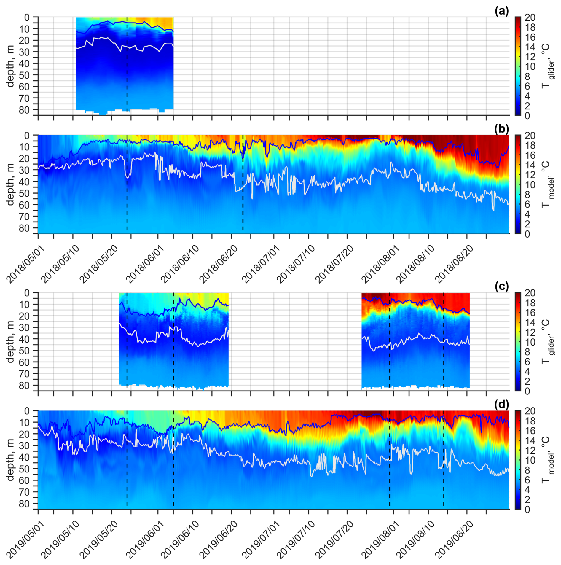
Figure 3 Temperature variability based on glider data (a, c) and model data (b, d) for May–August 2018 (a, b) and 2019 (c, d). The glider data represent average profiles for each section within the selected area, forming a composite temperature field. The model data show average profiles within a 1×1 km window at each model output time. Blue and white lines indicate the depths of the UML and the CIL, respectively. Vertical black lines indicate the dates shown in Fig. 8: 24 May and 23 June 2018 (a, b); 24 May, 5 June, 31 July, and 14 August 2019 (c, d).

Temporal developments of temperature and salinity distributions, stratification, and spice from the simulation and glider observations are shown in Figs. 3–6. A three-layered structure of the water column, consisting of a warm surface layer (upper mixed layer, UML), a cold intermediate layer (CIL), and a saltier deep layer, was observed and simulated. Observed patterns of variability in temperature and salinity distributions were well simulated by the model (Figs. 3 and 4). In absolute values, salinity was underestimated by 0.4 g kg⁻¹, while CIL temperatures were overestimated by approximately 2 °C in 2018 and 1.5 °C in 2019 in the model. In general, the model replicated the characteristic vertical density structure of the water column in the GoF and the development of the seasonal thermocline (Fig. 5). However, when characterizing the vertical structure and stratification of the water column, we point to some discrepancies.

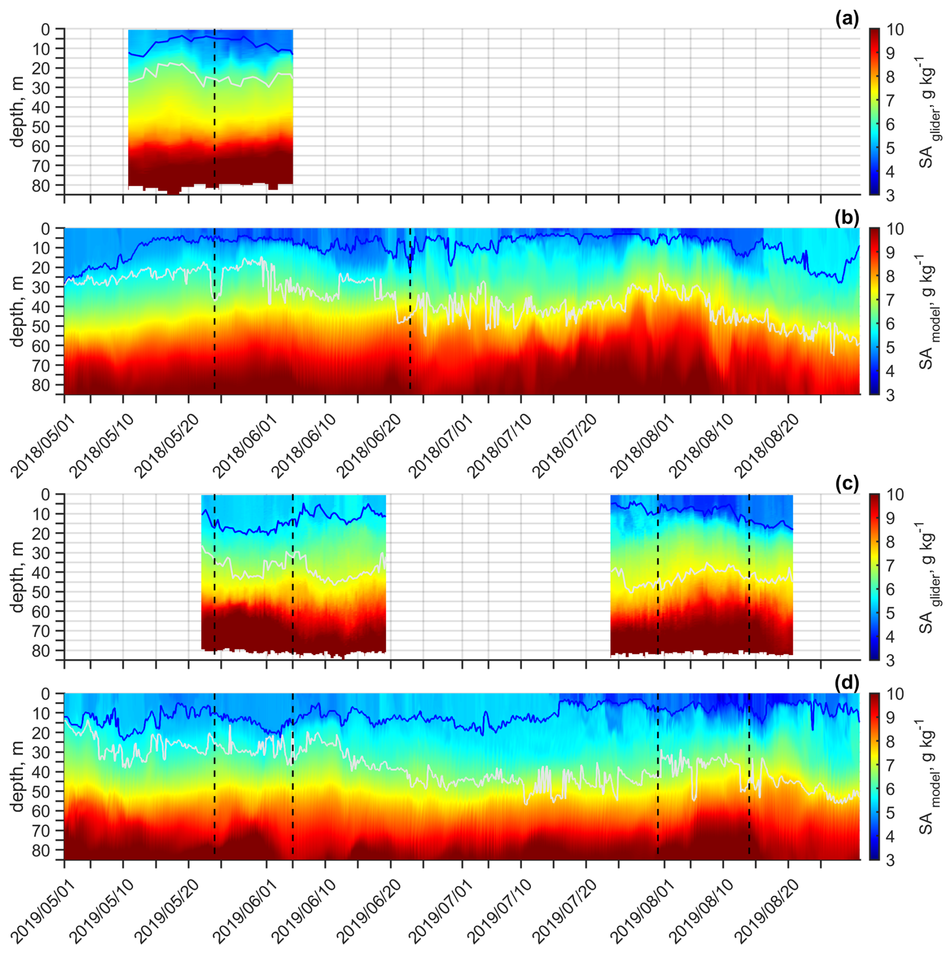
Figure 4 Salinity variability based on glider data (a, c) and model data (b, d) for May–August 2018 (a, b) and 2019 (c, d). The glider data represent average profiles for each section within the selected area, forming a composite salinity field. The model data show average profiles within a 1×1 km window at each model output time. Blue and white lines indicate the depths of the UML and the CIL, respectively. Vertical black lines indicate the dates shown in Fig. 8: 24 May and 23 June 2018 (a, b); 24 May, 5 June, 31 July, and 14 August 2019 (c, d).

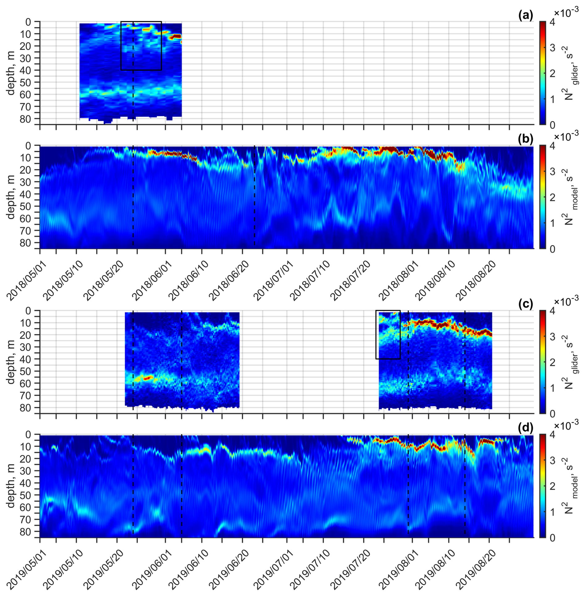
Figure 5 Variability of vertical stratification presented as Brunt–Väisälä frequency squared (N²) based on glider data (a, c) and model data (b, d) for May–August 2018 (a, b) and 2019 (c, d). The glider data represent average profiles for each section within the selected area, forming a composite salinity field. The model data show average profiles within a 1×1 km window at each model output time. Vertical black lines indicate the dates shown in Fig. 8: 24 May and 23 June 2018 (a, b); 24 May, 5 June, 31 July, and 14 August 2019 (c, d). Black boxes indicate periods of two observed local maxima in N²: 21–30 May 2018 (a) and 23–28 July 2019 (c).

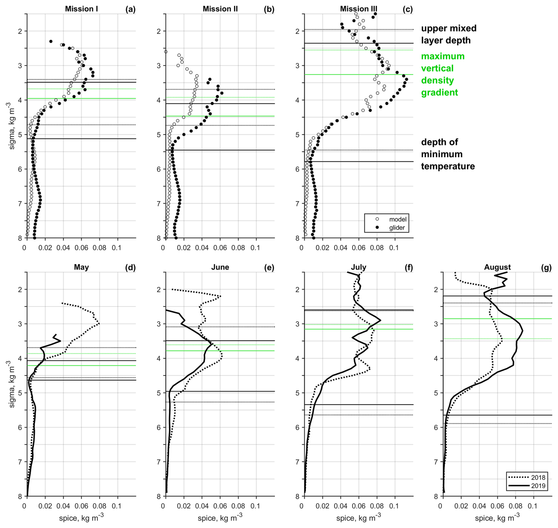
Figure 6 The standard deviation of spice. (a–c) First row: measured (black dots) and modelled (white circles) spice variability for each glider mission period. Solid and dashed black lines mark the average UML depth and depth of minimum temperature from measurements and model, respectively. Green lines indicate the average depth of maximum Brunt–Väisälä frequency. (d–g) Second row: monthly standard deviation of modelled spice from May to August in 2018 (dashed) and 2019 (solid). Black and green horizontal lines represent the same reference depths as in panels (a)–(c). All dashed lines correspond to 2018, and all solid lines to 2019. Model data were averaged over a 1×1 km area (see Fig. 1).

The observed and modelled UML depths were in close agreement during Missions I (7±3.7 and 7±3.1 m) and II (13±4.4 and 13±3.7 m) but diverged more in Mission III, with an observed average depth of 10±4.4 m compared to 6±2.6 m in the model. The depth of the CIL was reasonably well captured by the model in Missions I and III, with average observed and simulated depths of 22±5.0 and 24±5.5 m, and 43±5.2 and 41±6.0 m, respectively – both within the uncertainty of the estimates. However, a significant discrepancy was evident in Mission II, where the model placed the CIL approximately 10 m shallower than observed (29±5.1 m vs. 39±5.5 m).

The observed and simulated depths of the maximum N² were, respectively, 10±5.9 and 8±4.0 m during Mission I, 20±7.5 m and 15 m ± 4.1 m during Mission II and 14±4.8 and 9±3.2 m during Mission III. These differences, ranging from approximately 2 to 5 m, indicate a systematic underestimation of the depth of the strongest stratification in the upper water column by the model. Partly, this could be related to an overall weaker salinity gradient in the model compared to observations. For instance, in the first half of Mission II (spring 2019), the strongest vertical density gradient, as indicated by the maximum N², was determined by the vertical salinity distribution, as indicated by the glider data, whereas the model placed it shallower where the seasonal thermocline began to develop. Furthermore, the model did not capture the presence of occasionally observed two local maxima of N², e.g., on 21–30 May 2018 and 23–28 July 2019 (Fig. 5). On both occasions, glider observations revealed two distinct stratification peaks: respectively, at 7±2.7 m with the maximum N² of 0.0026±0.0005 s⁻² and at 19±4.2 m with 0.0016±0.0003 s⁻², and at 6±2.8 m with 0.0023±0.0007 s⁻² and at 19±2.5 m with 0.0023±0.0003 s⁻². The model showed a single stratification maximum of approximately 0.0017±0.0003 s⁻² at 6±2.6 m on 21–30 May 2018 and 0.0041±0.0008 s⁻² at 5±1.0 m on 23–28 July 2019. These discrepancies suggest that the model underrepresents the vertical complexity of stratification in the upper water column, the point that will be discussed in the Discussion section.

The halocline was generally weaker in the model during all missions (Fig. 5). However, as our focus is on the seasonal thermocline, we do not analyse this further and assume its impact on the upper-layer variability is minimal.

According to both the measurements and the simulation, spice intensity was highest during the summer 2019 mission (Fig. 6a–c), coinciding with the period of strongest vertical gradients in temperature, salinity, and density, and the most intense stratification (Figs. 3–5). The results, specifically the vertical distribution patterns of spice, were generally consistent between the model and observations; however, the model tended to underestimate the maximum spice intensities during spring missions. Nevertheless, both datasets point to a potential relationship between the development of stratification and SMS variability (processes). During the spring missions (May–June 2018 and 2019), spice maxima were located around the base of the UML. They occurred at shallower depths (corresponding to lower densities) than the depth of the maximum vertical density gradient. In contrast, during the summer mission (July–August 2019), the spice peak shifted to greater depths, situated beneath the UML and immediately below the strongest density gradient.

To extend this analysis, we present monthly average stratification parameters and vertical distributions of spice from model output for May through August 2018 and 2019 (Fig. 6d–g). The density range between the UML and the CIL increased from spring to late summer, indicating a deepening and strengthening of the pycnocline. Both the UML depth and the depth of the maximum density gradient shifted toward lower densities over the season, except in July–August 2018, when this trend was less pronounced. In May of both years, the maximum spice was at lower densities than those corresponding to the UML depth and the depth of the maximum density gradient. From June to August, the spice maxima aligned more closely with the density of the maximum vertical density gradient, suggesting a seasonal deepening of spice variability. Elevated spice intensities were spread over a broader density range over the summer months, reflecting the seasonal development of the pycnocline.

Further, in June 2018 and August 2019, a secondary local maximum of spice intensity was detected closer to the sea surface at low densities, indicating enhanced variability in the upper layer during these periods. This suggests that while the primary spice variability deepens with the season, episodic events can still induce significant variability in the upper layers.

Comparing the two years, 2019 exhibited a more pronounced seasonal progression in spice distribution, with a clearer deepening and broadening of the spice-rich layer from May to August. In contrast, 2018 showed a less consistent pattern, particularly in July–August, when the expected shift toward lower densities was not as evident. These interannual differences highlight the influence of varying atmospheric and oceanographic conditions on the seasonal development of spice variability.

3.2 Background forcing and large-scale and mesoscale dynamics

Background forcing in the study area in May–August 2018 and 2019 was characterized by mostly positive net surface heat flux (Q) and variable wind conditions (Fig. 7). Short periods of negative Q occurred in early June and July 2018, August 2018, early May and July 2019, and again in late July to early August 2019. Easterly and north-easterly winds, which favour upwelling along the southern coast of the GoF, were prevalent in July 2018 and also notable in May 2018 and May and July 2019 (Fig. 7a, c). Conversely, downwelling-favourable westerly and south-westerly winds dominated in June of both years. August wind patterns were marked by frequent southerly winds, while northerly winds were more common in July 2019. Wind speed rarely exceeded 10 m s⁻¹, except in June 2018, when three episodes of strong westerly winds occurred. These events led to vertical mixing and downwelling in the study area, resulting in deepening of the thermocline and weakened upper layer stratification. N² peaked in early June, decreasing from 0.006 s⁻² on 2 June to 0.002 s⁻² by 10 June, accompanied by a deepening of its maximum from 5 to 15 m (Fig. 5b). Similarly, downwelling-favourable winds and negative Q at the beginning of July 2019 contributed to reduced vertical stratification. The already weak stratification, characterized by a maximum N² of 0.002 s⁻² at 18 m depth, weakened further between 1 and 5 July, with the depth of the maximum shifting to 30 m (Fig. 5d). Several calm periods lasting about one to two weeks, namely in May and July of both years, allowed for the development and strengthening of vertical stratification. Substantial stratification strengthening occurred in May and July 2018, with N² maxima peaking at 0.006 and 0.01 s⁻², respectively (Fig. 5b). In contrast, by the end of July 2019, the N² maximum reached only 0.005 s⁻² (Fig. 5d). In August, SW–W winds dominated in both years, and Q was no longer predominantly positive.

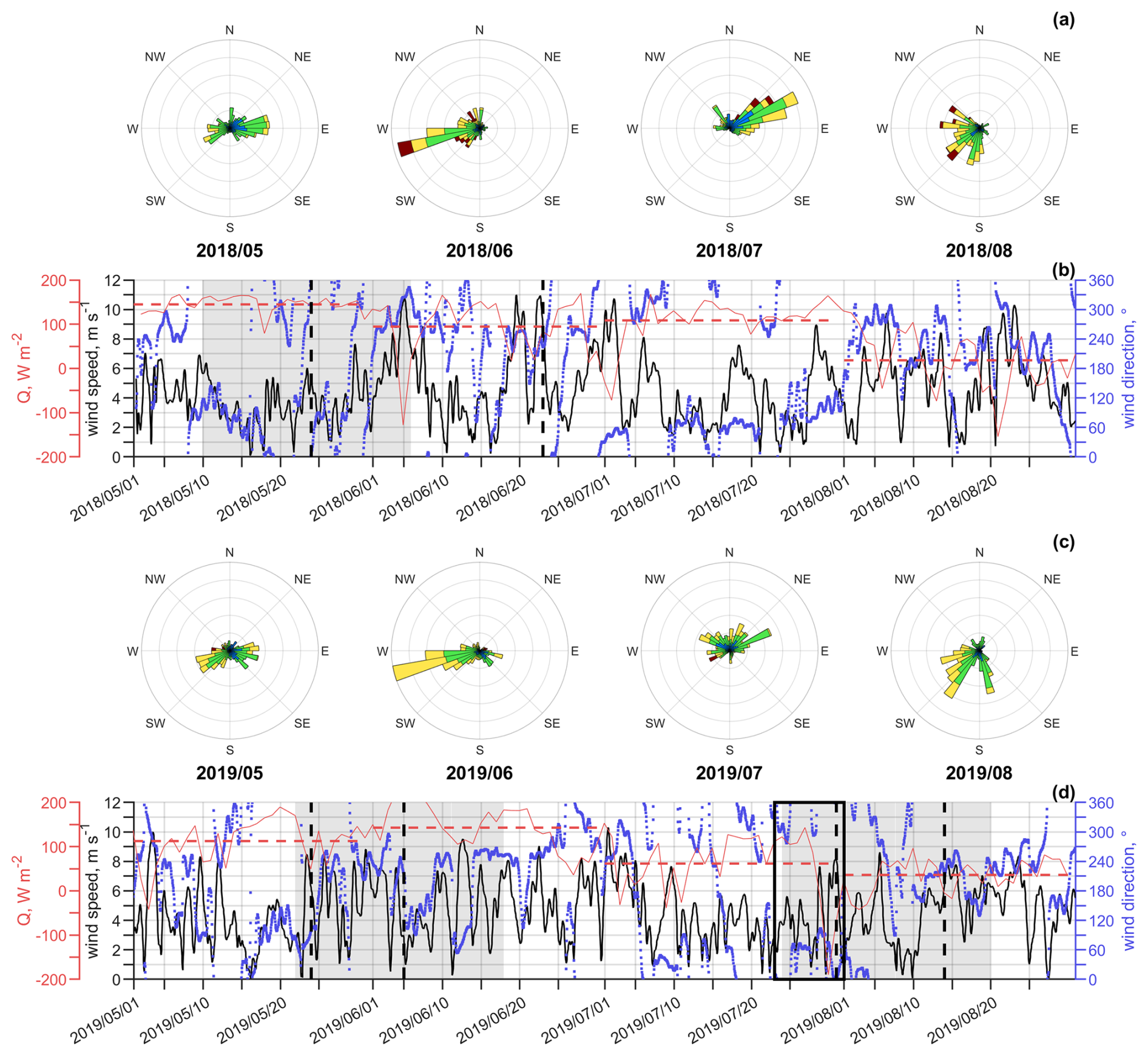
Figure 7 The daily average net surface heat flux, Q, (red, dashed line showing the monthly average), wind speed (black) and direction (blue) in spring–summer 2018–2019 (b, d). Panels (a) and (c) show the wind roses from May to August for both years, respectively. Vertical black lines indicate the dates shown in Fig. 8: 24 May and 23 June 2018 (b); 24 May, 5 June, 31 July, and 14 August 2019 (d). The black box indicates the period examined in Sect. 3.4: 23–31 July 2019 (d).

We suggest that wind forcing and surface heat flux played a crucial role in shaping the thermohaline variability in the area, with notable differences between the two years. To better illustrate how atmospheric forcing influenced the development of background hydrographic conditions, we present a series of characteristic events from spring–summer 2018–2019.

In May 2018, NE–E winds (Fig. 7b) triggered upwellings along the southern coast, evident in narrow coastal regions with low temperatures (Fig. 8a). Concurrently, a broader westward flow transported warmer, less salty surface water from the eastern GoF into the study area (Fig. 8a). In June 2018, strong SW–W winds led to downwelling along the southern coast (Fig. 8b), deepening the thermocline and altering the upper-layer structure.

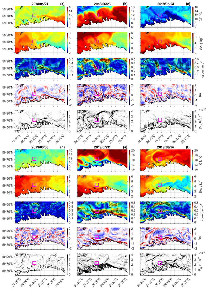
Figure 8 Overview of surface hydrographic and dynamical conditions in the Gulf of Finland during spring–summer 2018–2019, illustrating the variability of SMS-relevant fields. Example dates characterizing the evolving dynamical background are shown in (a–c) first row: 24 May 2018, 23 June 2018, and 24 May 2019, and in (d–f) second row: 5 June, 31 July, and 14 August 2019. For each date, panels from top to bottom display surface (0–3 m) Conservative Temperature (°C), Absolute Salinity (g kg⁻¹), velocity (m s⁻¹), Rossby number, and squared horizontal buoyancy gradient modulus (s⁻⁴). The magenta box marks the 10×10 km study window.

In May 2019, upwelling along the southern coast was more intense than in the previous year, driven by a strong E wind impulse on 22–23 May (Fig. 7d), resulting in pronounced cold water intrusions along the southern coast (Fig. 8c). By June 2019, upwelling subsided as SW–W winds became dominant, leading to the formation of mesoscale rotating structures in the central gulf (Fig. 8d). In late July 2019, NE–E winds over several days (Fig. 7d) once again caused upwelling along the southern coast, accompanied by a strong surface-layer outflow from the gulf (Fig. 8e). This outflow weakened in early August as northerly winds and negative Q prevailed (Fig. 7d). However westward advection of fresher water persisted, making the study area a transition zone between distinct water masses (Fig. 8f).

Overall, the dynamical background varied substantially across the study period, reflecting a strong influence of episodic atmospheric forcing. Depending on the prevailing wind conditions, mesoscale features such as upwellings and associated westward flows (Fig. 8a, c and e), downwellings (Fig. 8b), and eddies (Fig. 8d and f) developed. These features coincided with enhanced SMS activity, as evidenced by elevated Ro and intensified horizontal buoyancy gradients in the surface layer, particularly near frontal zones and filaments. In May 2018, May 2019, and July 2019 (Fig. 8a, c, and e), strong lateral gradients and Ro O(1) emerged near the southern coast, aligning with coastal upwelling. Further, the westward intrusion of low-salinity water from the eastern part of the gulf played a notable role in maintaining lateral density gradients across the basin, particularly in August 2019 (Fig. 8f). The SMS-active regions were more pronounced in summer (Fig. 8b, e and f), likely due to sharper lateral density gradients and a shallower mixed layer, that reduced the local Rossby deformation radius and favoured stronger SMS instabilities by intensifying frontal sharpness and enabling ageostrophic motions at smaller scales. Transient wind events and air–sea fluxes emerge as key drivers of mesoscale and SMS variability in the GoF, generating conditions that favour the development of SMS instabilities. The resulting SMS activity and its spatial distribution are examined in the following section.

3.3 Submesoscale variability from spice in observations and model

The intensity of SMS variability, quantified by the root mean square of spice, displayed multiple peaks throughout the spring–summer periods of 2018 and 2019. Some of these peaks coincided with elevated surface Ro variability (indicated by local maxima in the root mean square Ro; Fig. 9), such as during 25–27 July and early August 2018 or in August 2019, while others occurred under relatively low Ro conditions. Notably, high spice values were observed on 18 June and 11–13 July 2018, as well as between 22 and 30 July 2019, despite moderate to weak Ro variability (Fig. 9b and d). This partial decoupling suggests that spice may capture a broader spectrum of SMS variability, including processes less directly linked to elevated relative vorticity.

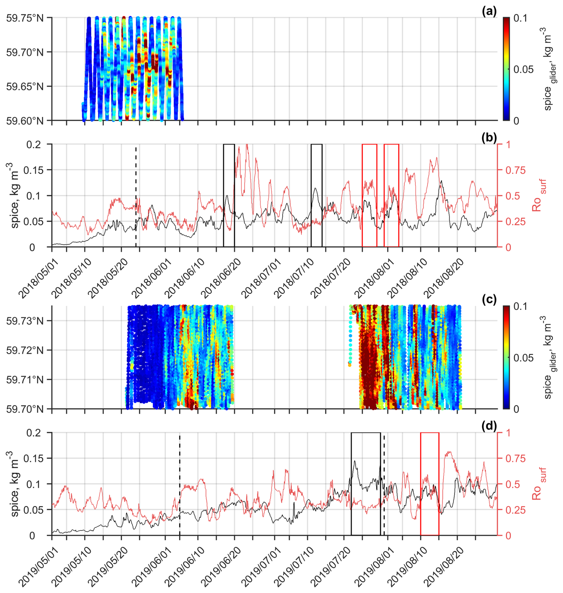
Figure 9 Root mean square spice in the density range from the surface to the depth of minimum temperature in spring–summer 2018–2019. Panels (a) and (c) show spice intensity along the glider trajectory; panels (b) and (d) show model results, calculated within a 10×10 km study window. The black line shows spice, and the red line indicates the surface root mean square Rossby number (Ro). Vertical black lines mark the dates shown in Fig. 10, corresponding to periods discussed in Sect. 3.3: 24 May 2018 (b), and 5 June and 31 July 2019 (d). Red boxes highlight example periods of high spice and high Ro, while black boxes indicate periods of high spice and low Ro (b, d).

Spice intensities from glider data and model data show good qualitative agreement, considering that the model values were averaged over the defined time series box (see Fig. 1; compare Fig. 9a and b, and Fig. 9c and d). Both datasets reveal an overall increase in spice intensity from May to August, reflecting the seasonal strengthening of stratification (which is at its maximum in July–August) and the intensification of background temperature and salinity gradients. This seasonal trend is further supported by a concurrent rise in Ro, punctuated by transient peaks driven by episodic strong wind forcing, as in late June 2018 (Fig. 9b).

We selected three periods when both glider and model data were available to demonstrate how the distribution of parameters indicative of SMS instabilities/processes relates to spice. The intensification of spice observed in the second half of May 2018 (Fig. 9a) and simulated by the model (Fig. 9b) coincided with the eastward transport of warmer, less saline water and the formation of horizontal buoyancy gradients (Fig. 8a). During 15–25 May, calm weather prevailed, and Ro, averaged over the time series box, exhibited a sustained increase towards O(1), indicating enhanced SMS activity in the surface layer. The spice intensity concurrently increased, with notable peaks on 18 and 25 May, and reached its maximum on 28 May (Fig. 9b). Figures 8a and 10d demonstrate the presence of elongated SMS structures on 24 May, characterized by Ro O(1), Ri<1, and relatively strong horizontal buoyancy gradients. Elevated spice intensity was located near these features, indicating enhanced thermohaline variability associated with SMS instabilities (Fig. 10d).

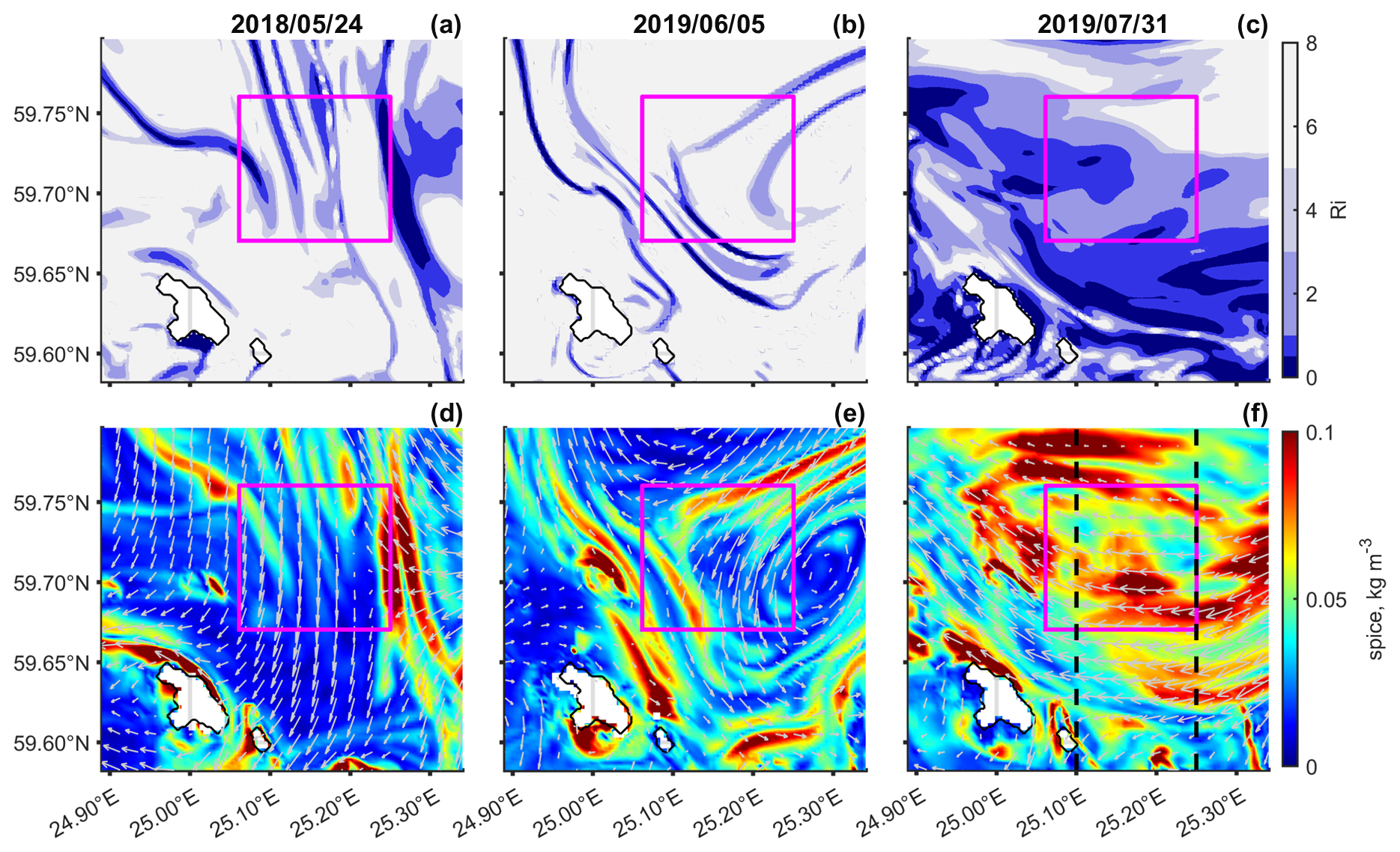
Figure 10 Richardson number (a–c) and root mean square spice calculated within the density layer from the surface to the depth of minimum temperature (d–f) during spring–summer 2018–2019. Each column shows one example date from a different glider mission period – 24 May 2018, 5 June and 31 July 2019 – corresponding to the dates shown in Fig. 8. The magenta box marks the 10×10 km study window.

In late May 2019, an intense upwelling occurred along the southern coast (e.g., 24 May; Fig. 8c). However, this did not lead to a notable increase in the spice intensity or Ro within the time series box (Fig. 9d). A considerable rise in Ro and modest rise in spice intensity occurred at the beginning of June, coinciding with a change from SW winds on 1 June to SE winds on 5 June (Fig. 7d). During this period, a cyclonic eddy (∼10 km in diameter) formed in the study area, accompanied by a larger anticyclonic eddy offshore (Fig. 8d). Elevated Ro from 5 to 11 June indicated the persistence of this cyclonic feature in the time series box (Fig. 9d). Elevated spice intensity was observed at the periphery of the cyclonic eddy (Fig. 10e), aligned with narrow stripes of relatively high buoyancy gradients and low Ri (Figs. 8d and 10b).

High spice intensity observed during the third week of July 2019 (Fig. 9c and d) appeared to be associated with varying wind forcing (Fig. 7d) and the development of a westward current along the southern coast of the GoF (Fig. 8e). Westerly winds at the beginning of July were followed by upwelling-favourable winds on 7–10 July, which evoked the westward coastal current. After that, a period of weaker variable winds followed, and then another stronger pulse of easterly winds occurred, further strengthening the coastal current. Despite the dynamic conditions, Ro within the time series box remained relatively low during this period (Fig. 9d). However, Fig. 8e reveals that regions of Ro O(1) and strong horizontal buoyancy gradients linked to the coastal current were located just south of the study area. Interestingly, patches of low Ri appeared also north of the region with the highest surface current speeds, while areas of high spice intensity were found even farther north (Fig. 10c and f). The observed spatial offsets between Ro, Ri, and spice intensity suggest that active SMS processes may be vertically and/or laterally displaced from the surface frontal zone. These patterns motivate a closer inspection of the late July period.

3.4 Upwelling-driven submesoscale variability and subduction

The period from 23 to 31 July 2019 was selected for closer analysis due to an observed peak in spice variability (Fig. 9d). For each day within this period, a set of vertical sections, as shown in Fig. 11, was produced (Figs. S1–S9). Prior to the strong easterly wind impulse on 28–29 July, winds varied between NE and NW, averaging 3.5 m s⁻¹ (Fig. 7d). After 25 July, the easterly wind component strengthened, and by 26 July 2019, a strong coastal current had emerged, accompanied by high subsurface variability in temperature and salinity across all three selected sections (Figs. S3 and S4). This current intensified by 29 July, coinciding with a clear upwelling event. Surface temperatures dropped from 22 °C, and northward velocities increased sharply in the upper layer (Fig. 11a–d). Isopycnals tilted, with an outcropping of the 3 kg m⁻³ isopycnal (Fig. 11f), reflecting enhanced horizontal buoyancy gradients and frontal sharpening – conditions favourable for SMS instabilities.

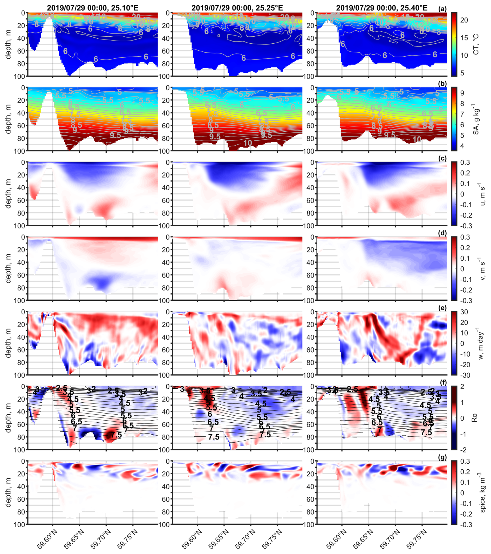
Figure 11 Vertical sections along three meridional transects at 25.10, 25.25, and 25.40° E on 29 July 2019, showing (a) Conservative Temperature (°C), (b) Absolute Salinity (g kg⁻¹), (c) zonal velocity u (m s⁻¹), (d) meridional velocity v (m s⁻¹), (e) vertical velocity w (m d⁻¹), (f) Rossby number (Ro) with overlaid isopycnals (0.25 kg m⁻³ intervals), and (g) spice (kg m⁻³). Transect locations are shown in Fig. 12f.

Ro reached O(1) near the coastal current zone and topographic features (Fig. 11f) while remaining relatively low in the offshore area (left panel in Fig. 11f and Ro curve in Fig. 9d). Vertical velocities increased notably across all transects (Fig. 11e), and horizontal velocity fields indicated intensified shear in the upper 40 m (Fig. 11c and d). These dynamics are consistent with shear-driven instability and frontal subduction.

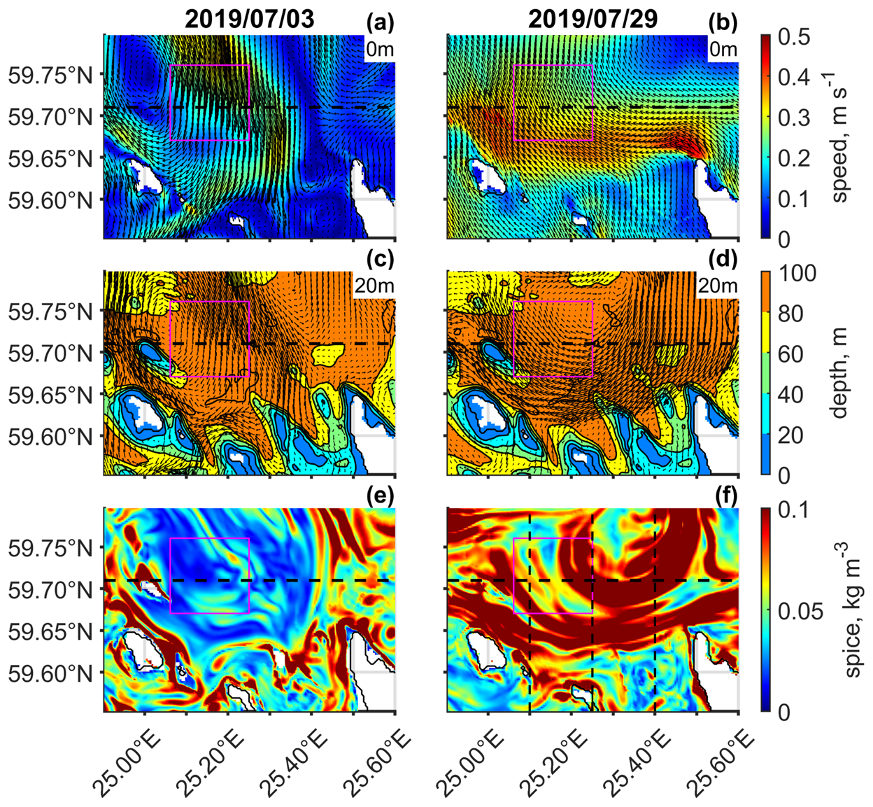
Figure 12 Comparison of surface and subsurface conditions between 3 July (a, c, e) and 29 July 2019 (b, d, f). Panels (a) and (b) show surface horizontal velocity (m s⁻¹), panels (c) and (d) velocity vectors at 20 m depth overlaid on bathymetry, and panels (e) and (f) root mean square of spice anomaly (kg m⁻³) in the density range limited from the surface to the depth of minimum temperature. The magenta box marks the 10×10 km study window. The horizontal black lines indicate the zonal transect shown in Fig. 13. The vertical black lines in panel (f) indicate the meridional transects shown in Figs. 11 and S1–S9.

By 29 July, spice anomalies became more confined to the upper 15 m and showed weaker spatial alignment with elevated Ro (Fig. 11g), in contrast to 27–28 July, when enhanced subsurface spice was more closely aligned with regions of Ro O(1) (Figs. S5 and S6). Notably, spice extended beyond the core of the coastal current, with elevated values observed near sloping isopycnals and beneath frontal zones (Fig. 11g). These signals, aligned with tilted isopycnals, indicate both vertical and lateral thermohaline displacement.

Horizontal distributions of velocity and spice at the surface and 20 m depth (Fig. 12) highlight the influence of flow–topography interactions on SMS variability. At the surface, the coastal current veered offshore at several locations, particularly downstream of peninsulas and bathymetric irregularities (Fig. 12b). At 20 m, flow patterns differed significantly from the surface, especially near the coast where the flow reversed with depth, indicating strong vertical shear (Fig. 12b and d). Elevated spice intensity near these transitions (Fig. 12f) suggests that such flow structures contribute to the generation and modulation of SMS features. Spice intensity was highest both along the coast and in offshore areas where the coastal current deflected seaward, especially westward (downflow) of coastal and topographic irregularities.

We compared the patterns in the case of upwelling described above with those observed during downwelling conditions in early July 2019. On 3 July, the surface current field was characterized by prevailing shoreward transport and the presence of eddies in the surface layer (Fig. 12a). The flow at 20 m roughly mirrored the surface (Fig. 12c), indicating weaker vertical shear, although localized shear zones were still present near topographic features. High spice intensity was present nearshore and, to a lesser extent, offshore (Fig. 12e), but overall spice intensity was lower than on 29 July.

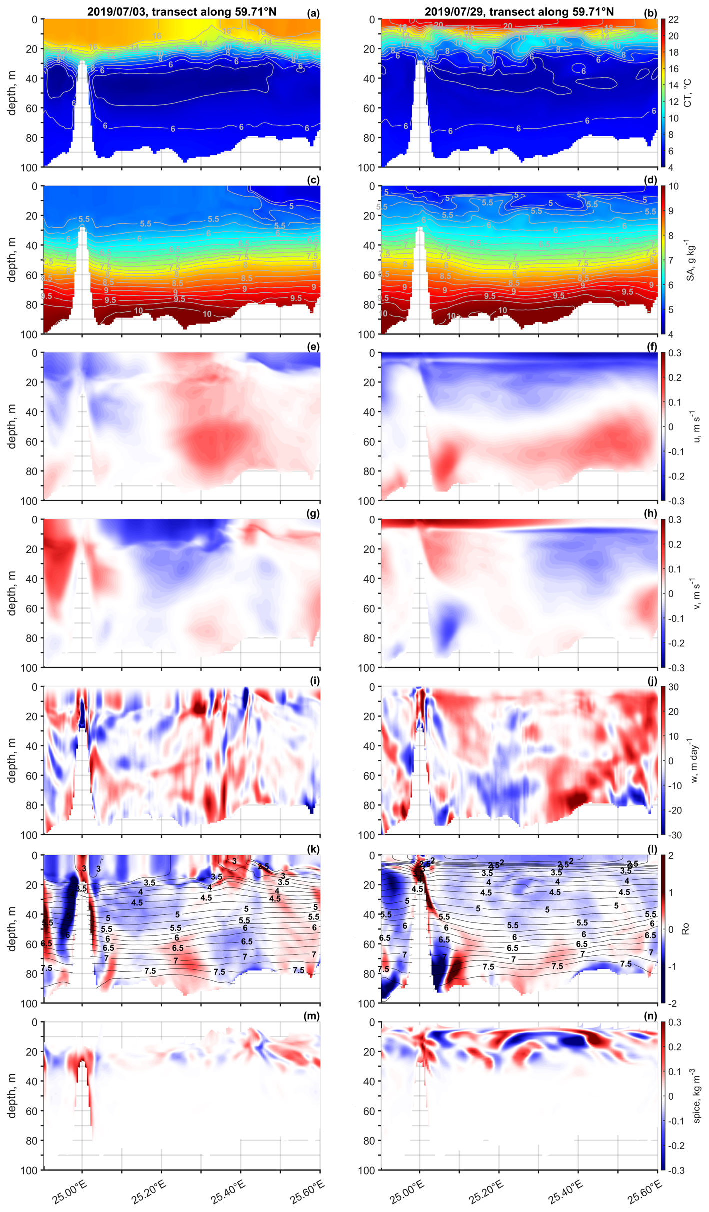
Figure 13 Vertical sections along zonal transects at 59.71° N on 3 July (a, c, e, g, i, k, m) and 29 July 2019 (b, d, f, h, j, l, n), showing (a, b) Conservative Temperature (°C), (c, d) Absolute Salinity (g kg⁻¹), (e, f) zonal velocity u (m s⁻¹), (g, h) meridional velocity v (m s⁻¹), (i, j) vertical velocity w (m d⁻¹), (k, l) Rossby number (Ro) with overlaid isopycnals (0.25 kg m⁻³ intervals), and (m, n) spice (kg m⁻³).

This contrast is further illustrated by zonal cross-sections (Fig. 13), which provide an alongshore view of the thermohaline and dynamic structure during the two events. While the transects from 3 and 29 July share some structural similarities, they also reveal key dynamic differences. Due to the alongshore orientation and its distance from the coast, signs of upwelling are more difficult to detect directly. However, meridional sections (Figs. S1–S9) confirm the presence of upwelled water, indicated by surface temperatures below 20 °C and salinities near 5 g kg⁻¹ on the 29 July transect (Fig. 13b and d). In contrast, during downwelling on 3 July, thermohaline gradients were weaker, and the thermocline was deeper, centred around 20 m (Fig. 13a and c). The different flow structure was noticeable. On 29 July, offshore flow was evident in the surface layer, particularly between 24.9 and 25.3° E (Fig. 13f and h). On 3 July, the current exhibited shoreward flow from the surface to 20 m depth, especially between 25.0 and 25.4° E (Fig. 13e and g).

Both dates showed Ro O(1) near the topographic feature at ∼25.0° E (Fig. 13k and l). The enhancement of spice near this location suggests that coastal topography persistently acts as a hotspot for SMS generation (Fig. 13m and n). However, under upwelling conditions, these features become more dynamic and spatially extensive, amplifying thermohaline variability. Offshore Ro values remained generally low on 29 July (Fig. 13l). Interestingly, a frontal zone was beginning to develop in the 25.15–25.25° E region on 3 July (Fig. 13k), highlighting the localized and incipient character of SMS activity under downwelling conditions. Near this structure, vertical velocities were enhanced (Fig. 13i), and a modest increase in spice was seen (Fig. 13m). On 29 July, vertical velocities were more spatially extensive and intensified above sloping topography (Fig. 13j), where enhanced interlayer exchange likely contributed to the observed spice. Spice were more intense and penetrated deeper into the water column on 29 July (Fig. 13n), reflecting both vertical and lateral redistribution of thermohaline properties, consistent with subduction and frontal advection. While meridional sections showed spice becoming more confined to the upper 15 m near the coast (Fig. 11g), the zonal transect revealed broader lateral displacement along the frontal zone.

This comparison of late July upwelling and early July downwelling conditions highlights how wind forcing and topography modulate SMS activity in the GoF. Both periods were governed by stable summer stratification, and recurrent SMS features were observed near topographic structures. However, the upwelling event on 29 July triggered sharper horizontal density gradients, stronger vertical shear, elevated Ro, and more extensive vertical velocities. These conditions favoured frontal instabilities, subduction, and lateral advection, resulting in deeper, more structured spice. In contrast, the downwelling regime on 3 July exhibited weaker gradients and more localized, surface-confined SMS signals. Together, vertical sections and horizontal maps reveal how frontal processes and flow–topography interactions jointly control the intensity and extent of SMS variability.

4 Discussion

While satellite imagery has revealed widespread SMS variability at the sea surface in the Baltic Sea (e.g., Lavrova et al., 2018), the vertical structure and dynamics of SMS processes remain underexplored, particularly from observational datasets. In this study, we built upon earlier glider-based observations (Salm et al., 2023), which revealed subsurface SMS variability and highlighted the value of high-resolution autonomous measurements. We extend this work by combining observational data with numerical simulations to examine the structure and variability of SMS features more comprehensively. This combined approach provides insight into the three-dimensional nature of SMS processes and enabled us to identify clear spice-based SMS signatures in the subsurface layers, co-located with regions of Ro O(1) and Ri<1 (Figs. 8a, d, e and 10), pointing to active SMS instability and mixing processes. To our knowledge, this is the first study to apply this integrated approach to investigate SMS dynamics in the GoF.

The complex physical environment of the Baltic Sea is known to pose a challenge for numerical models, often resulting in biases in the simulated salinity and/or temperature fields, as well as inaccuracies in capturing the pycnoclines correctly (e.g., Gröger et al., 2022; Hordoir et al., 2019; Liblik et al., 2020; Väli et al., 2013). In this study, we showed that the model with the SMS-permitting grid spacing could simulate the development of the vertical structure of the water column and the SMS variability reasonably well. The general patterns of spice variability were consistent between measurements and simulation. The UML depth was also well captured, and the CIL was accurately reproduced during Missions I and III. However, during Mission II, the model underestimated the depth of the CIL by approximately 10 m and systematically underestimated the depth of the maximum N², with the largest discrepancy again occurring during Mission II (Fig. 5). Furthermore, the model did not capture the presence of occasionally observed two local maxima of N². These discrepancies could be related to difficulties in simulating salinity distributions in this basin (see, e.g., Westerlund et al., 2018). At the beginning of Mission I (spring 2018), the seasonal thermocline was almost absent (Fig. 3), and the salinity gradient defined the vertical density gradient. On the mentioned two occasions of two local N² maxima, the deeper one was largely determined by salinity, as detected by the glider. We suggest that the model does not simulate salinity distributions (which are mainly related to the large-scale advection and mixing of freshwater and saltier water) as accurately as temperature distributions (which are mostly defined by local atmospheric forcing).

Despite these limitations, the model successfully captured the key SMS patterns and associated frontal structures, providing a reliable basis for interpreting the observed events and tracer distributions. Note, for instance, the identical vertical location of the highest spice intensity in relation to the UML depth and strongest density gradient in observations and model results (Fig. 6a–c). During spring missions, the spice maximum was situated at the base of the UML, but shallower than the strongest density gradient. During the summer mission, it was located just below the strongest density gradient. Similarly, Chrysagi et al. (2021) showed that a GETM simulation could replicate the structure of an observed cold SMS filament.

To interpret the SMS structures, we employed spice as a tracer. Spice, which varies from cold and fresh to warm and salty, provides a dynamically passive tracer. We defined spice through along-isopycnal temperature and salinity anomalies with respect to the spatial mean considering typical internal Rossby deformation of 4 km. While some studies compute spice across all spatial scales corresponding to the dataset to examine the spectral properties (e.g., Jaeger et al., 2020; Klymak et al., 2015), our scale-dependent definition emphasizes SMS variability by revealing patchy thermohaline structure near regions of Ro O(1) and elevated vertical velocities (e.g., Fig. 11).

Spice was consistently observed during all glider missions and throughout the modelling periods from May to August 2018 and 2019. Spice intensity tended to increase as the upper layer warmed and the seasonal thermocline developed. We argue that the observed spatial and temporal peaks in spice intensity, against the backdrop of an overall increasing trend, indicate instances with high activity of SMS processes.

Analysis of spice intensity revealed that tracer patches in the vertical structure appear as horizontally elongated features (bottom rows in Figs. 10 and 12), closely matching the estimated dimensions of SMS structures (∼10–20 km long, ∼1 km wide) reported by Zhurbas et al. (2022). That study also suggested a vertical decoupling between SMS processes in the UML and those below. Our findings support this conceptual separation, showing that in summer months, SMS features frequently occurred below the UML (Fig. 6c), often decoupled from elevated surface Ro (Fig. 9).

Furthermore, in early June 2019, the simulation showed a small cyclonic vorticity whose periphery was outlined by elevated spice (Fig. 10b and e), consistent with observations by Yang et al. (2017), who linked such eddy peripheries with intensified mixing. These results indicate the potential of spice to reveal instances of SMS-driven energy transfer toward smaller scales.

Recent studies have shown that surface heating can suppress SMS flows, while surface cooling promotes them. However, favourable wind forcing can still enhance SMS activity under surface heating conditions (Peng et al., 2021; Shang et al., 2023). Changes or reductions in wind forcing can also trigger SMS frontal instabilities that lead to restratification of the UML, as shown by glider measurements and simulations in the Baltic Sea (Carpenter et al., 2020; Chrysagi et al., 2021; Salm et al., 2023). The development of SMS flows depends critically on horizontal buoyancy gradients (e.g., Bosse et al., 2021; Ramachandran et al., 2018;), which in GoF arise from multiple sources (e.g., Lips et al., 2016a). Predominantly positive Q promotes stratification in spring and early summer, although at different rates in coastal and open sea areas (e.g., Lips et al., 2014). Wind forcing influences the inclination of the thermocline (Liblik and Lips, 2017), while upwelling and downwelling events effectively form strong horizontal temperature, salinity and density gradients in spring–summer (e.g., Kikas and Lips, 2016). These lateral buoyancy gradients provide the energy that drives SMS processes (Boccaletti et al., 2007).

We suggest that the SMS spice maxima observed above the maximum vertical density gradient in spring, under conditions of positive Q and weak wind forcing, reflect SMS processes acting to restratify the deeper portion of the UML. The secondary peaks of spice near the sea surface in June 2018 and August 2019 (Fig. 6e and g) could be linked to a characteristic forcing pattern during these months – strong wind mixing events were followed by a period of weaker winds and positive Q. These results suggest that the SMS processes can contribute to restratifcation both near the sea surface (under positive Q) and at the base of the UML, driven by lateral buoyancy gradients, as also noted by Miracca-Lage et al. (2024). Oceanic studies have similarly demonstrated that SMS processes can strongly influence mixed layer depth (e.g., du Plessis et al., 2017), and our findings support this by showing that SMS processes (defined by spice-based signals) play a direct role in shaping the vertical stratification. This highlights the importance of resolving SMS variability in coastal models to improve predictions of stratification evolution and coastal–offshore exchanges.

Conversely, cooling (negative Q) and wind-induced turbulence contribute to the deepening of the UML. However, SMS processes can also emerge below the UML and the maximum vertical density gradient, as observed in July–August 2019, when both wind and Q were more variable. Dove et al. (2021) reported that deepening of the mixed layer in regions of high eddy kinetic energy coincided with increased spice and oxygen concentrations below the mixed layer. In our data, elevated subsurface spice in July–August 2019 did not align with the elevated Ro at the sea surface, but rather with the presence of a baroclinic coastal current. A particular example occurred at the end of July. The situation with Ro O(1) near the topographic features and outcropping isopycnals was characterized by high spice in the offshore subsurface layer (Fig. 11f and g) and intensification of vertical velocities, indicating SMS frontal subduction beneath the upwelling front (Fig. 11e). These signals, aligned with tilted isopycnals, indicate both vertical and lateral thermohaline displacement. The apparent decoupling between spice and Ro patterns likely reflects the downstream advection and transformation of SMS features beyond their generation sites, supporting a scenario of shallow subduction driven by persistent frontal tilting and vertical shear. Similar subduction along the slanted isopycnals associated with the SMS activity at the upwelling front has been described by Hosegood et al. (2017). Capo et al. (2023) further suggested that flow-topography interactions generate vorticities, which are transported offshore in the subsurface layers.

Our results from July 2019 highlight how coastal upwelling and downwelling regimes distinctly modulate SMS variability in the offshore subsurface layer (Figs. 12 and 13). Winds favourable for upwelling (downwelling) in the southern GoF strengthen (weaken) vertical stratification and move the pycnocline upward (downward) towards the coast (Liblik and Lips, 2017). Coastal downwelling likely favours vertical turbulent mixing by reducing vertical stratification, making SMS features less visible. If SMS subduction occurs under these conditions, tracer patches are likely to be transported shoreward along slanted isopycnals beneath the downwelling-related baroclinic current. It explains a similar localized intensification of spice near the topographic features under upwelling- and downwelling-dominated conditions but with considerably weaker offshore SMS variability in the case of downwelling. This suggests that while topographic features consistently support SMS generation, upwelling enhances frontal subduction and the lateral spread of SMS structures into the basin's interior. Such upwelling-related SMS subduction acts counter to the mesoscale secondary circulation, which typically exhibits offshore surface flow and onshore subsurface return flow.

SMS subduction at fronts may contribute to the dissipation of mesoscale kinetic energy and downward transport of tracers (Archer et al., 2020), including the formation of subsurface chlorophyll maxima (e.g., Hofmann et al., 2024). By transporting phytoplankton-rich surface waters downward along sloping isopycnals, SMS processes can facilitate biomass accumulation below the pycnocline, as observed during summer in connection with anticyclonic circulation cells and SMS intrusions (Lips et al., 2010, 2011; Ruiz et al., 2019). Future analysis of collected glider data from the region, along with a comparison of spice variability with subsurface chlorophyll patchiness, could help to understand better the SMS processes and their biogeochemical impact in the Baltic Sea and similar stratified basins.

5 Conclusions

This study demonstrates that SMS variability in the Gulf of Finland is strongly modulated by both atmospheric forcing – particularly surface heat flux and wind stress – and background hydrographic structures such as mesoscale frontal gradients. Glider observations, supported by high-resolution modelling, revealed consistent spatial patterns of SMS activity, with SMS spice concentrated near the UML base in spring and within the thermocline in late summer, demonstrating the vertical sensitivity of SMS features to seasonal stratification. Wind forcing became dominant to shape the distribution of SMS anomalies when surface buoyancy input was weak. High SMS variability and subduction signatures were consistently found on the offshore side of a baroclinic coastal current, where sloped isopycnals aligned with velocity and SMS spice indicated downward and lateral transport of surface-layer waters. The integration of observations and model output allowed for extrapolation beyond individual glider transects, confirming that SMS processes in this coastal sea are both dynamically active and responsive to variations in external forcing. These results suggest the physical mechanisms that govern SMS variability and subduction in stratified coastal environments. Further studies, including high-resolution observations and modelling, are needed to understand SMS dynamics better and assess their biogeochemical consequences.