Leading dynamical processes of global marine heatwaves in an ocean state estimate

Marine heatwaves (MHWs) have emerged as a very active area of research due to the devastating impacts of these events on marine ecosystems across different trophic levels. However, a clear understanding of the local drivers of these extreme ocean conditions is still limited at a global scale. Observations of the terms needed to constrain ocean heat budgets are very sparse, ocean reanalysis products are generally non-conservative and inadequate to conduct accurate heat budget analyses, and the fidelity of climate models with respect to simulating MHWs is still unclear. In this study, we make use of Argo float observations, a satellite-based sea surface temperature product, and the Estimating the Circulation and Climate of the Ocean (ECCO) state estimate to assess MHW characteristics over the global ocean. ECCO is then used to evaluate local MHW drivers. ECCO assimilates observations using the adjoint methodology, which optimizes the system trajectory given the observational constraints in a conservative fashion, making it an ideal product for the estimation of heat budgets. The representation of MHWs in ECCO is generally consistent with observations, although ECCO tends to underestimate MHW frequency and intensity and overestimate duration, relative to the observational products. Atmospheric forcing emerges as the dominant contributor to MHW onset and decline across most regions, while ocean dynamics, including the advective and diffusive convergence of heat, play crucial roles in the equatorial regions, specifically in the extratropical zones (e.g., western boundary currents, such as the Gulf Stream and Kuroshio) and the Southern Ocean. Regional analyses in the northeastern Pacific, southwestern Pacific, and Tasman Sea show diversity in leading dynamical mechanisms for MHW onset and decline both across regions and across events in the same regions: while air–sea exchanges of heat may contribute most frequently to MHW onset and decline, other mechanisms can also often provide dominant contributions and, at times, be the main driver. A more complete understanding of MHWs and their drivers is crucial for predicting their initiation, duration, intensity, and decline, to ultimately inform the development of mitigation and adaptation strategies for affected communities.

1 Introduction

Events of extreme warming in the ocean have received increasing attention due to their profound ecological and socioeconomic impacts (Smith et al., 2021), as they are often associated with widespread ecosystem disruptions (Guo et al., 2022; Smith et al., 2023), coral bleaching (Brown, 1997; Donovan et al., 2021), shifts in species distributions (Lonhart et al., 2019), and changes in oceanic primary productivity (Frölicher and Laufkötter, 2018; Pearce et al., 2011). A better understanding of these extreme events and how they will affect marine ecosystems and livelihoods in the future is crucial to help coastal communities adapt to them.

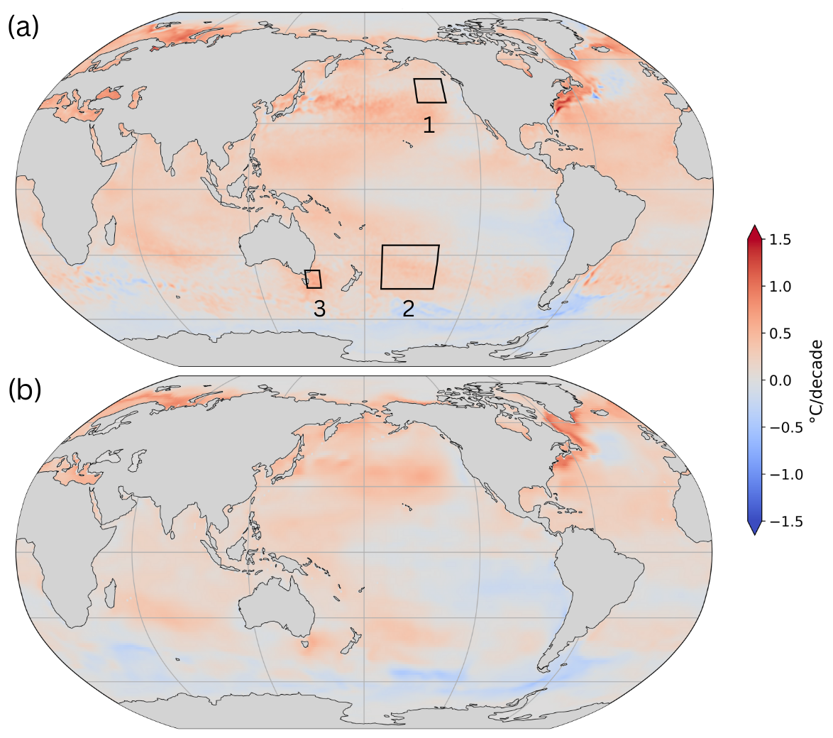
Figure 1 Linear trend in (a) sea surface temperature based on the NOAA OISST V2 data product and (b) near-surface temperature from the ECCO v4r4 ocean state estimate (°C per decade). The trend is estimated from monthly data over the period from 1992 to 2017. Boxes in panel (a) also show the regions of interest in our analysis: (1) the northeastern Pacific, (2) the southwestern Pacific, and (3) the Tasman Sea.

Extreme warm conditions associated with processes internal to the climate system occur in the presence of a long-term global warming trend (Fig. 1), which can increase their frequency of occurrence and intensity and exacerbate their impacts. While atmospheric greenhouse gas concentrations are nearly spatially uniform, the long-term warming of the ocean surface shows regional patterns that affect the atmospheric circulation, regional changes in rainfall, and the global climate sensitivity (Xie, 2020). Both the distribution of radiative forcing (greenhouse gas vs. aerosols concentrations) and the ocean circulation (e.g., global overturning circulation, wind-driven circulation, and upwelling) shape observed patterns (Xie, 2020), leading, for example, to long-term warming signals in the area of the western boundary currents (Fig. 1; Wu et al., 2012). The presence of this large sea surface temperature (SST) trend has led to discussions on appropriate definitions of marine heatwaves (MHWs) in a changing climate (Amaya et al., 2023; Burrows, 2023). Specifically, MHW definitions that do not factor out the effects of having a trend in the data, e.g., those based on a fixed baseline to define the climatology used to assess extremes (Hobday et al., 2016) lead to an increase in the frequency and intensity of these extreme events (Seneviratne et al., 2021; Wigley, 2009; Evans et al., 2020; Oliver et al., 2018; Oliver, 2019; Smale et al., 2019; Scannell et al., 2016; Xu et al., 2022) and may also result in permanent MHW conditions in regions of accelerated warming (Capotondi et al., 2024). The inclusion of the long-term trend in MHW definitions can also be expected to confound our understanding of the processes leading to MHW development as well as their associated predictability (Wulff et al., 2022). On the other hand, impact studies may need to consider the total SST anomalies, especially when they are concerned with marine species that have a slow adaptation timescale (Smith et al., 2024). The implications of different MHW definitions and their suitability for different applications are discussed in depth in Smith et al. (2024).

In this paper, we aim at understanding the processes underpinning MHW events arising from internal climate processes, due, for example, to an increase in variance (Xu et al., 2022). In particular, variability associated with the El Niño–Southern Oscillation (ENSO) appears to increase the likelihood and/or persistence of MHWs in different parts of the world (Frölicher and Laufkötter, 2018; Oliver et al., 2018; Sen Gupta et al., 2020; Xu et al., 2021; Capotondi et al., 2022; Gregory et al., 2024a), suggesting that changes related to ENSO could account for a substantial portion of the future increase in MHWs (Deser et al., 2024; Capotondi et al., 2024). A better understanding of the different drivers of MHWs in different regions of the ocean can help improve MHW forecasts and the information that policymakers use to develop proactive mitigating strategies (Holbrook et al., 2019, 2020). Local atmospheric processes and oceanic circulation patterns play critical roles in shaping the dynamics of MHWs as well as their intensity and duration (Pujol et al., 2022; Marin et al., 2022). Teleconnections from large-scale modes of variability can play an important role in modulating the local drivers, as seen in events like the 2013–2015 northeastern Pacific MHW, known as “the Blob” (Di Lorenzo and Mantua, 2016).

While a large fraction of the literature has focused on the development phase of MHWs, the processes responsible for the demise of these events are also important. Thus, here we consider drivers of both the onset and decline phases of MHW events (Fig. 3) during 1992–2017. For this purpose, we use, for the first time in MHW studies, the Estimating the Circulation and Climate of the Ocean (ECCO) state estimate. This dynamically consistent ocean state estimate incorporates a wide range of oceanic and atmospheric observations (Forget et al., 2015) and provides daily temperature fields, as well as all heat budget terms computed at each model time step, ensuring closure of the heat budget. We note that the attribution of heat budget terms, particularly the separation of advective and diffusive contributions, is inherently tied to model resolution, and coarse-resolution products may misattribute unresolved advective processes to subgrid-scale diffusion. However, while eddy-permitting (∼0.25°) or eddy-rich (∼0.1°) models improve MHW realism in highly dynamic regions (e.g., western boundary currents), even coarser-resolution models can qualitatively capture large-scale MHW patterns in less active regions (Pilo et al., 2019). While ECCO's 1×1° resolution is a limitation, results from (observation-constrained) ECCO results provide an excellent complement to results from free-running models (of comparable resolution) described in recent MHW studies, such as work using the CESM large ensemble (1–1.5°; Deser et al., 2024) and an analysis based on the GFDL ESM2M coupled Earth system model (with a nominal 1° resolution increasing (in longitude) to $\mathrm{1}/\mathrm{3}$° near the Equator) describing MHW dynamics and local drivers of MHW onset and decline phases in different seasons over a 500-year period (Vogt et al., 2022). ECCO provides an optimal balance between resolution, dynamical fidelity (thanks to being constrained by observations), and spatial coverage for global, process-based MHW analysis. Furthermore, compared to other data-assimilating products, ECCO enables heat budget closure – an essential advantage for our process-focused analysis. In this work, our goals are to (1) describe MHW characteristics in ECCO relative to satellite-based and in situ observations and (2) investigate the roles of oceanic and atmospheric drivers of MHWs over the global ocean, providing valuable insights for ecosystem management, climate adaptation strategies, and sustainable resource planning. Data and methods used in our analysis are described in Sects. 2 and 3, respectively. Results and discussion are presented in Sect. 4. Conclusions are drawn in Sect. 5.

2 Data

2.1 ECCO v4r4 ocean state estimate

We use data from Version 4 Release 4 (v4r4) of the ECCO (Estimating the Circulation and Climate of the Ocean) ocean reanalysis from 1992 to December 2017. ECCO v4r4 is a conservative and dynamically consistent reanalysis based on the MIT general circulation model (Marshall et al., 1997) configured with 50 vertical levels and with a horizontal resolution of 1° throughout the globe. The ECCO ocean state estimate includes observational data used to constrain the model, e.g., from Argo floats, moorings, ship-based measurements (e.g., CTDs – conductivity–temperature–depth sensors), and satellites. We use ECCO potential temperature, salinity, heat and freshwater flux fields, and both daily and monthly output to examine how the definition of MHW characteristics is influenced by the temporal resolution of the data used.

2.2 Argo OHC

We use monthly ocean heat content (OHC) fields (for the 15–50 dbar layer) based on Argo profile data (Wong et al., 2020). In Giglio et al. (2024), Argo observations are mapped on a 1×1° grid using locally stationary Gaussian processes defined over space and time, with data-driven decorrelation scales (Kuusela and Stein, 2018). Furthermore, a linear time trend is included in the estimate of the mean field, along with spatial terms and harmonics for the annual cycle. We use mapped fields for the period from 2004 to 2017, which overlaps with the monthly ECCO data.

2.3 NOAA OISST V2

We use sea surface temperature data from the NOAA Optimum Interpolation Sea Surface Temperature (OISST) V2 High Resolution Dataset at a $\mathrm{1}/\mathrm{4}$° resolution (Huang et al., 2021) for the period from 1992 to 2017. This product has been extensively used by previous researchers for MHW identification, and it has the advantages of a high horizontal resolution and the availability of data at a daily timescale.

3 Methods

3.1 Marine heatwave identification

As in Hobday et al. (2016), marine heatwaves are identified here based on deviations from a time-evolving “normal” sea surface temperature (or upper-ocean heat content) that exceed a certain threshold over a specified period. This threshold is set as the seasonally varying 90th percentile, meaning that MHWs are characterized by sea surface temperature (or upper-ocean heat content) anomalies that are warmer than 90 % of anomalies in each season over a time frame of interest (for daily data, the seasonally varying 90th percentile is defined daily, using an 11 d moving window). Anomalies are defined with respect to the seasonal cycle and linear trend during the total duration of the period considered. Thus, unlike Hobday et al. (2016), who used the 1982–2012 fixed baseline, here we use the entire period for the definition of the climatology after removing the linear trend.

For MHWs to be identified, the anomalies in temperature (or ocean heat content) need to exceed the selected threshold for more than a minimum duration, to ensure that short-lived fluctuations in temperature or ocean heat content are not categorized as MHWs and that only long-lived thermal anomalies are included in the analysis. The minimum duration of MHW events is set based on the time resolution of each dataset, with 1 month for monthly data and 5 d for daily data. For daily data, the end of the event corresponds to anomalies remaining below the threshold for more than 2 d (after the initial 5 d of continuous anomalies above the threshold); i.e., we treat two MHW events separated by less than 2 d as a single, continuous MHW event. This approach is consistent with Hobday et al. (2016) and prevents the misclassification of prolonged MHWs as multiple shorter events, allowing us to maintain the continuity of the thermal anomaly and better reflect the actual duration and intensity of the events in our analysis.

Once the percentiles are calculated and the MHW thresholds are applied, we can identify the start and end dates of each event, track their evolution, and analyze their duration. Additionally, when using daily data, we can identify the MHW onset vs. decline phase, with the onset phase going from the start of the event to the peak intensity (included) and the decline starting just after the peak intensity and going to the end of the event (Fig. 2). By explicitly defining different phases, we can study processes driving MHW intensification and dissipation.

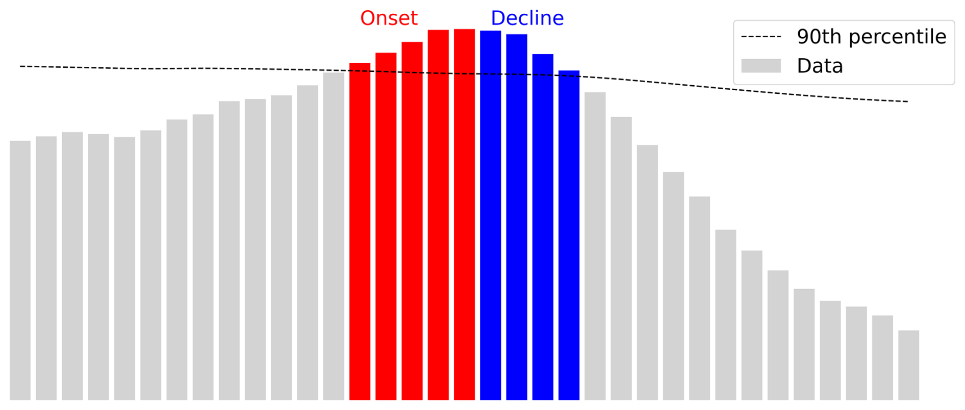
Figure 2 Schematic representing how we define and identify MHWs and their onset (red) and decline (blue) phases.

Finally, using daily data, we compare the statistics of MHWs of different durations, i.e., MHWs lasting between 5 and 29 d and events lasting 30 d or longer. In addition, as some previous studies have utilized monthly averaged data, especially in the case of long-lasting events like the Blob (Xu et al., 2022; Capotondi et al., 2022), here we also compare the statistics obtained using monthly averages with those derived from daily data.

3.2 ECCO ocean heat budget

To compute the global ocean heat budget in the upper ocean (5–55 m), we use the ECCO v4r4 product at daily and monthly resolutions, following the methodology outlined in Forget et al. (2015). The evolution of temperature is expressed as follows:

$$\begin{array}{}\text{(1)}& {\displaystyle \frac{\partial \mathit{\theta }}{\partial t}}=-\mathrm{\nabla }\cdot \left(\mathit{\theta }\mathit{u}\right)-\mathrm{\nabla }\cdot {\mathbf{F}}_{\mathrm{diff}}^{\mathit{\theta }}+{\mathbf{F}}_{\mathrm{forc}}^{\mathit{\theta }},\end{array}$$

where $\frac{\partial \mathit{\theta }}{\partial t}$ is the rate of change in potential temperature; $-\mathrm{\nabla }\cdot \left(\mathit{\theta }\mathit{u}\right)$ is the advective divergence term (encompassing both horizontal and vertical components of heat transport); $-\mathrm{\nabla }\cdot {\mathbf{F}}_{\mathrm{diff}}^{\mathit{\theta }}$ is the diffusive divergence term; and ${\mathbf{F}}_{\mathrm{forc}}^{\mathit{\theta }}$ denotes the atmospheric forcing term, including surface heat fluxes.

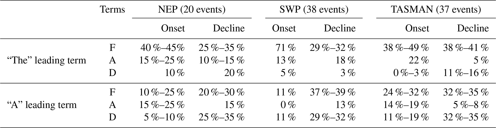
Ocean heat budget terms follow from the terms in this equation, as ocean heat content is the volume integral of $\mathit{\theta }\cdot \mathit{\rho }\cdot c_p$, where density ρ is 1030 kg m⁻³ and specific heat c_p is 3989.244 J(kg⁻¹ K⁻¹), as described in McDougall and Barker (2011). We note that the ECCO ocean heat budget closes almost exactly, as residuals are orders of magnitude smaller than the other budget terms. We compute composite fields for each heat budget term (atmospheric forcing, advective convergence, and diffusive convergence) separately during the onset and decline phases of marine heatwaves (MHWs), examining the relative contributions of these terms to ocean heating and cooling during the two phases (Fig. 7). To assess how often each term contributes to warming during MHW onset and cooling during MHW decline, we compute the frequency of positive (average) contributions during onset and negative (average) contributions during decline (Fig. 8). Furthermore, we evaluate how often each term is the largest or smallest contributor to the heat budget during each phase (Figs. 9 and 10), e.g., calculating the percentage of instances (across all the events) when a term is the largest contributor, regardless of how similar to other terms it may be. Towards summarizing our global and regional findings for the leading dynamical processes driving MHWs, we introduce the terms “the” leading term and “a” leading term, as explained in the following. For each phase, we identify the budget terms that contribute to it (among forcing, advective convergence, and diffusive convergence), and we then sort them by the magnitude of the contribution. A term provides “the” leading contribution if it exceeds the next largest term by at least 30 %. A term also provides the leading contribution if it is the only process contributing to the phase of interest. If the largest two contributors are both greater than the third by at least 30 % but neither is larger than the other by 30 %, each of the two terms provide “a” leading contribution. The same happens if these two terms are the only contributors and neither is larger than the other by 30 %. If none of the terms provide a contribution that is 30 % larger than other contributions, all three terms contribute comparably. We note that while the 30 % threshold is arbitrary, it serves the purpose of summarizing our results and visually identifying which processes are most often leading terms. Our findings are robust to ±5 % change in the (30 %) threshold percentage used (not shown) In addition to the global analysis, we perform a regional analysis, averaging heat budget terms and ocean heat content anomalies in three regions of the Pacific Ocean: the northeastern Pacific (region 1 in Fig. 1a, NEP), the southwestern Pacific (region 2, SWP), and the Tasman Sea (region 3, TASMAN). We evaluate the cumulative sum of each heat budget term during the onset and decline phases of MHW events, to estimate their contributions to OHC changes (e.g., identifying “a” leading term vs. “the” leading term), and show how the relative importance of the different processes varies across regions and events in the same region (Figs. 11–13).

4 Results and discussion

4.1 Representation of MHWs in ECCO compared to observations

ECCO provides an overall good representation of the spatial patterns of both the long-term linear trend in upper-ocean temperature (e.g., Fig. 1) and the 90th percentile anomalies (Fig. S1 in the Supplement); moreover, spatial patterns of MHW frequency, average duration, and average intensity in ECCO are consistent with observations (Figs. 3–6). However, a smaller number of near-surface MHW events shorter than a month (i.e., duration of between 5 and 29 d) are seen in ECCO compared to observations (Fig. 3a and d), with only some of these events showing a signature in upper-ocean (5–55 m) heat content (Fig. 3g). Some of the differences between ECCO and observations may be related to ECCO's resolution: Pilo et al. (2019) show that, while model configurations with resolutions ranging from 1 to $\mathrm{1}/\mathrm{10}$° can all qualitatively represent broad-scale global patterns in MHWs, modeled MHWs tend to be weaker, longer-lasting, and less frequent than in observations, especially for models with a lower resolution. High-resolution, eddy-permitting models perform generally better with respect to representing MHW characteristics, particularly in dynamic regions like the western boundary currents, but still exhibit biases (Pilo et al., 2019). Discrepancies between models and observations are due, in part, to smoother SST time series and longer autocorrelation times (Cooper, 2017) in models (compared to observations), which can reduce short-lived variability and emphasize events of longer duration.

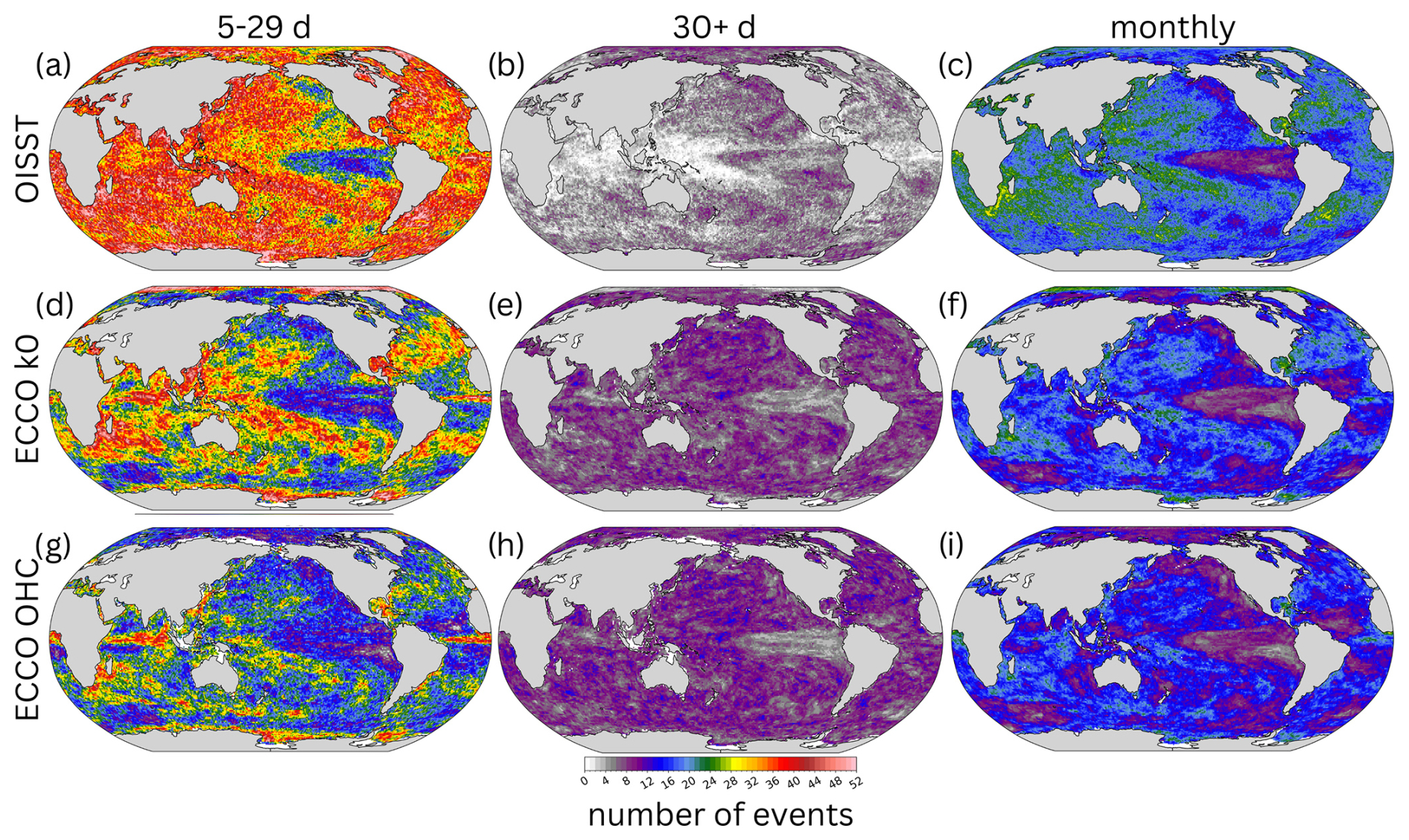
Figure 3 Total number of MHW events detected during the period from 1992 to 2017 using (a–c) SST V2 data, (d–f) ECCO v4r4 near-surface temperature, and (g–i) ECCO v4r4 ocean heat content (5–55 m). Panels (a), (b), (d), (e), (g), and (h) are based on daily data and include MHW events with a duration of (a, d, g) 5–29 d and (b, e, h) 30 or more days. Panels (c), (f), and (i) are based on monthly data and include MHW events with a minimum duration of 1 month.

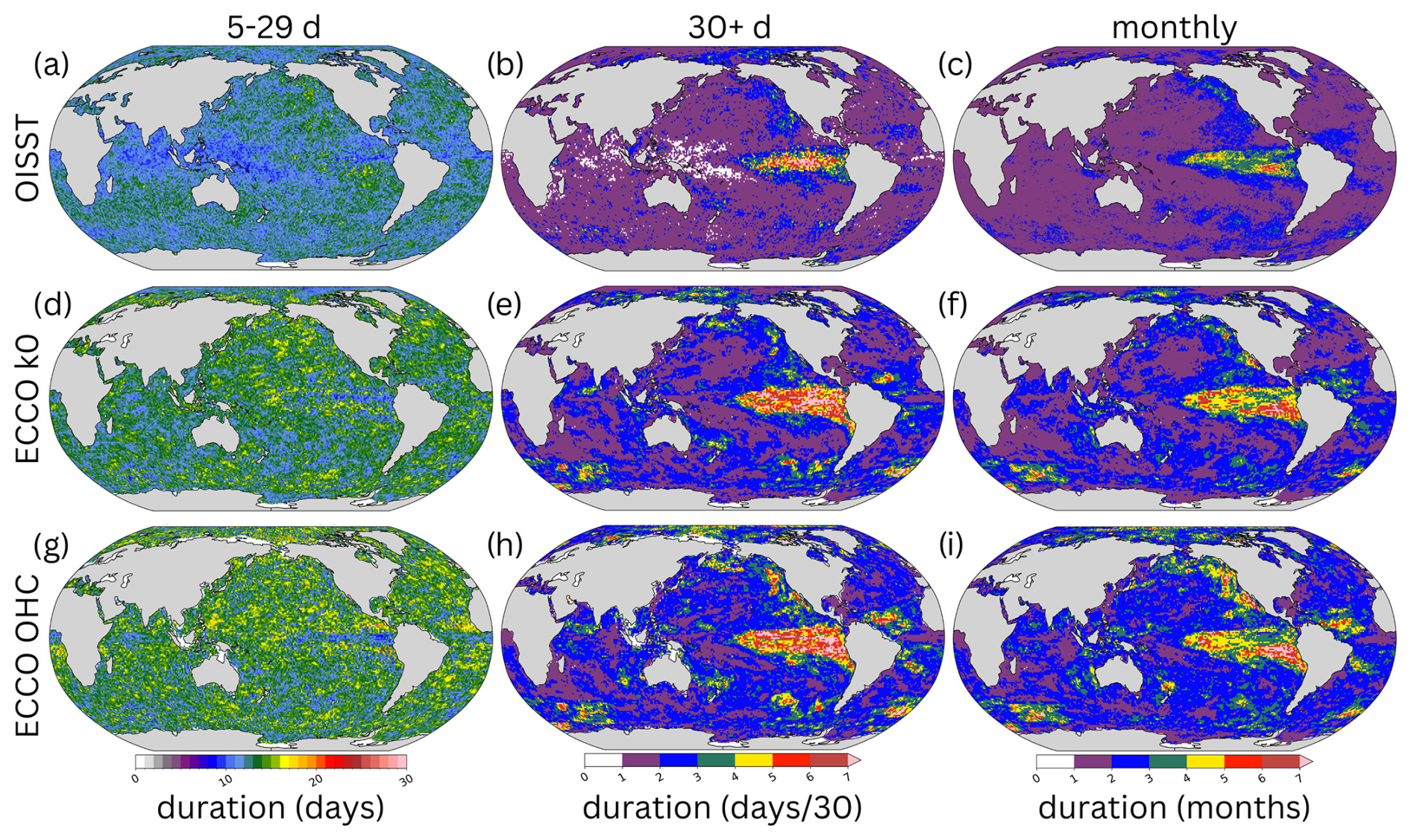
Figure 4 Same as Fig. 3 but for the average duration of MHW events.

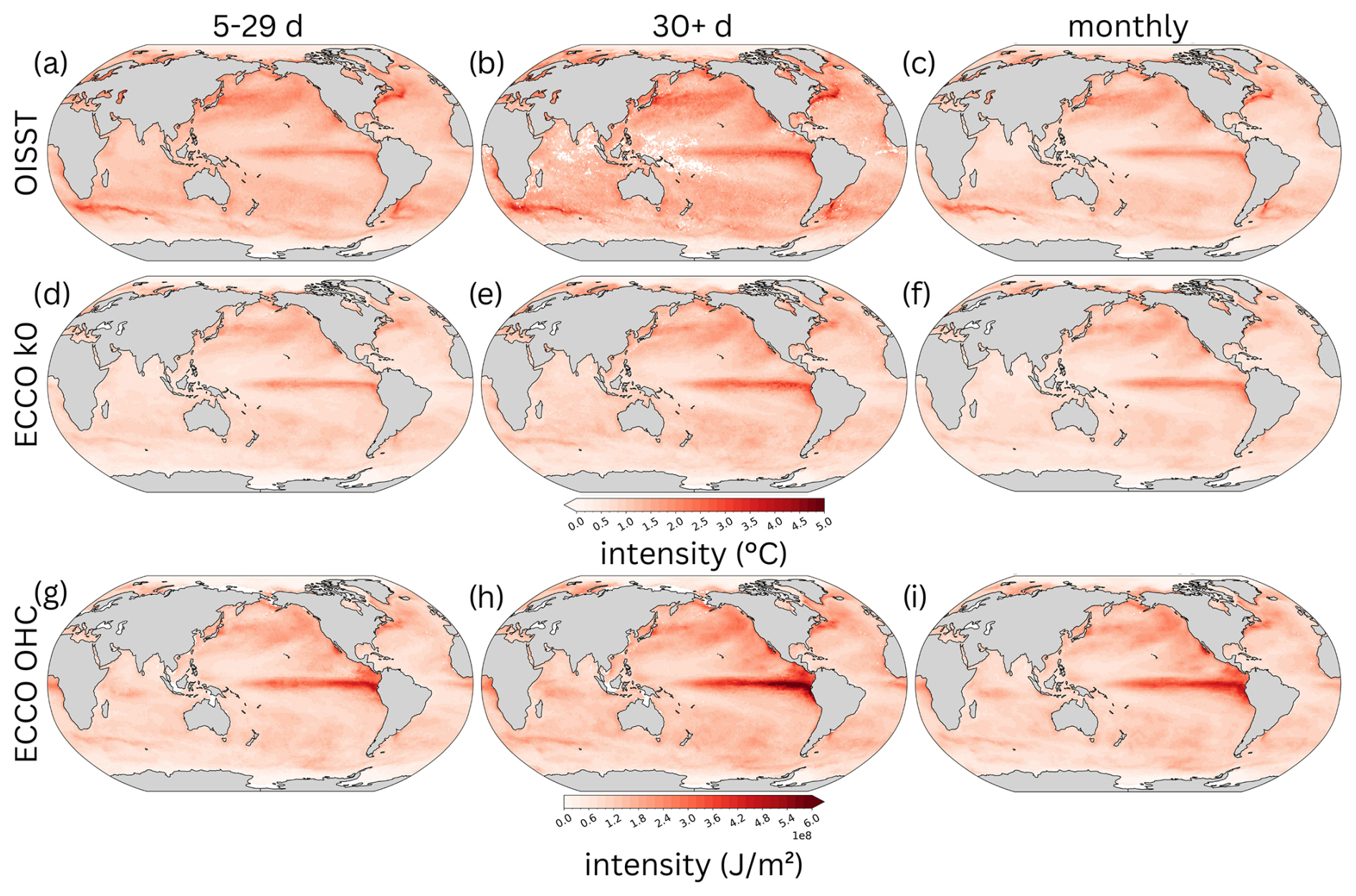
Figure 5 Same as Fig. 3 but for the average intensity of MHW events. Values in panels (a)–(f) have units of degrees Celsius (°C), whereas values in panels (g)–(i) are expressed as joules per square meter (J m⁻²).

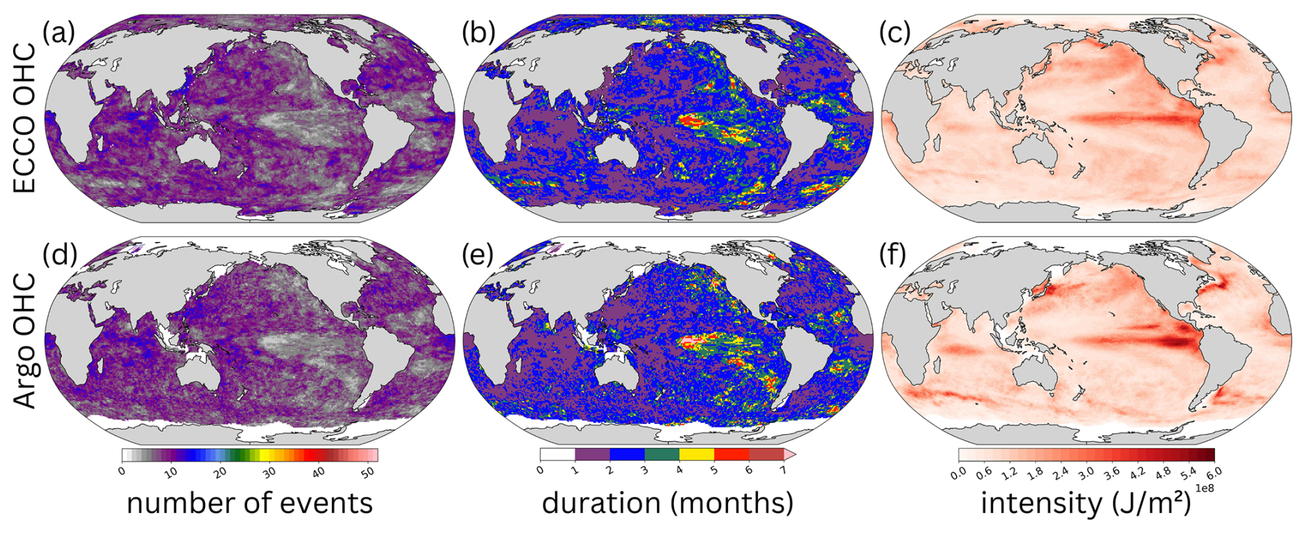
Figure 6 Number (a, d), duration (b, e), and intensity (c, f) of MHW events from 2004 to 2017 detected using ECCO v4r4 ocean heat content between 5 and 55 m (a–c) and Argo ocean heat content between 15 and 50 dbar (d–f).

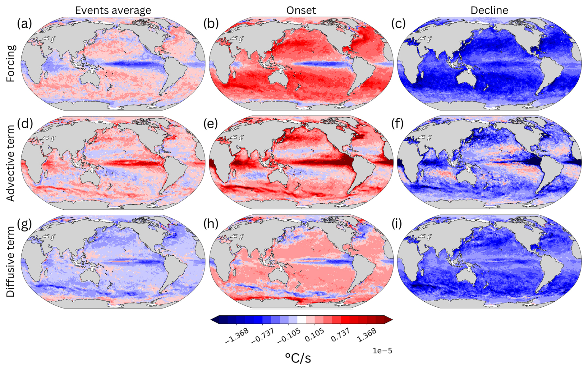
Figure 7 Average heat budget terms across MHW events with a minimum duration of 5 d, based on ECCOv4r4 upper-ocean (5–55 m) heat content: for each event, the average is computed during the whole event (a, d, g), the onset phase (b, e, h), and the decline phase (c, f, i). Panels (a)–(c) show atmospheric forcing, panels (d)–(f) show the advective convergence of heat, and panels (g)–(i) show the diffusive convergence of heat.

Despite the limitations highlighted above, ECCO provides a useful representation of MHWs in the global ocean. Furthermore, the availability of ECCO daily fields allows us to study dynamical mechanisms of MHWs during the onset and decline phase of the event. In the following, the analysis will focus on MHWs with a minimum duration of 5 d, without distinguishing between events lasting 5–29 d and those lasting 30 or more days, as results from the two categories are similar (not shown).

4.2 Leading dynamical processes for MHWs

In most of the ocean, the composite amplitude of atmospheric forcing during MHW onset and decline is larger than the amplitude for advective and diffusive convergence (Fig. 7b and c). The spatial distribution of this term is quasi-uniform, with the exception of the tropics. Atmospheric forcing contributes to warming during the onset phase and cooling during the decline (i.e., it is positive during the onset and negative during the decline phase) in most regions of the global ocean and for most events (Figs. 8 and 9); however, on average, atmospheric forcing cools the upper ocean during both the onset and decline phase near the Equator (Fig. 7b and c). In addition, it contributes to the decay most of the time (Fig. 8a and b), consistent with previous studies (Holbrook et al., 2019; Vogt et al., 2022). In equatorial regions, advective convergence plays a lead role in the onset and decline of MHW (and ENSO) warm anomalies (Figs. 9c and d and 10a–d), consistent with ENSO dynamics (e.g., Jin, 1997; Capotondi, 2013). On average, advective convergence contributes to both the onset and decline phase only near the Equator (Fig. 7e and f); in the subtropics and western boundary currents, consistent with previous studies (e.g., Li et al., 2022; Zhang et al., 2023); in the southern Red Sea and Gulf of Aden (Nadimpalli et al., 2025); and along the Antarctic Circumpolar Current (Fig. 7e and f). In these regions, the advective convergence is most often a contributor only to the onset phase (Fig. 8c), except for the eastern equatorial Atlantic and Pacific and the southern Red Sea and Gulf of Aden where it is most often also a contributor to the decline phase (Fig. 8d). As the composite amplitude of atmospheric forcing and advective convergence are similar between MHW onset and decline, the composite event average amplitude for each resembles the positive vs. negative patterns described for the onset (except values are much smaller; Fig. 7a and d). The patterns for the composite event average amplitude of diffusive convergence (Fig. 7g) are instead similar to what is seen for the decline phase (Fig. 7h), as, while the duration of the decline phase is on average shorter, the composite amplitude of diffusive divergence (i.e., negative values of diffusive convergence, corresponding to heat loss) is larger for the decline phase (Fig. 7i). The spatial patterns of the composite amplitude of diffusive convergence during MHW onset and decline are similar to what described for atmospheric forcing (except during the onset phase in proximity of western boundary currents and the Antarctic Circumpolar Current), yet values for diffusive convergence are smaller (Fig. 7h and i) and diffusive divergence is most often a contributor globally only to the decline phase, being a leading term at high latitudes (Fig. 9e and f). On average, the amplitude of diffusive divergence during the decline phase is larger in regions characterized by strong oceanic fronts, such as western boundary currents and the Antarctic Circumpolar Current (Fig. 7i). In these areas, diffusive processes help dissipate warm anomalies, suggesting that turbulent mixing is a key mechanism in reducing excess heat and restoring thermal equilibrium (Oliver et al., 2021; Vogt et al., 2022). While diffusive convergence is generally not a leading term for MHW onset (except near Antarctica), there are events when this happens, indicating that a variety of leading dynamical mechanisms are seen in most regions. Moreover, diffusive convergence contributes to the onset phase most often in some of the tropics, off the Equator (Fig. 8e and f).

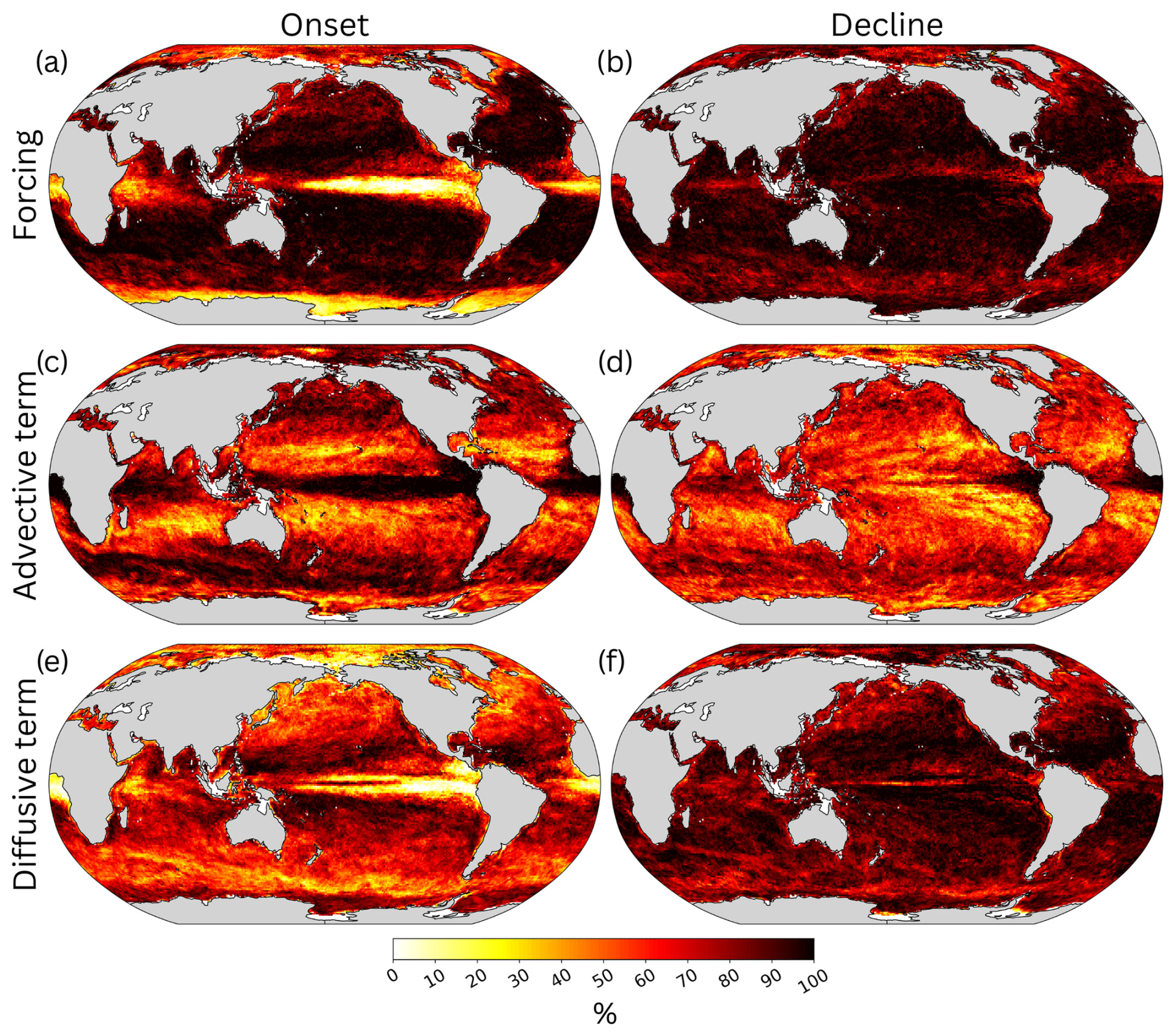
Figure 8 Percentage of times each heat budget term contributes to (a, c, e) the MHW onset phase and (b, d, f) the MHW decline phase, based on ECCOv4r4 upper-ocean (5–55 m) heat content. A budget term contributes to the onset phase if it is positive or to the decline phase if it is negative. Percentages are shown for (a, b) atmospheric forcing, (c, d) advective convergence of heat, and (e, f) diffusive convergence of heat.

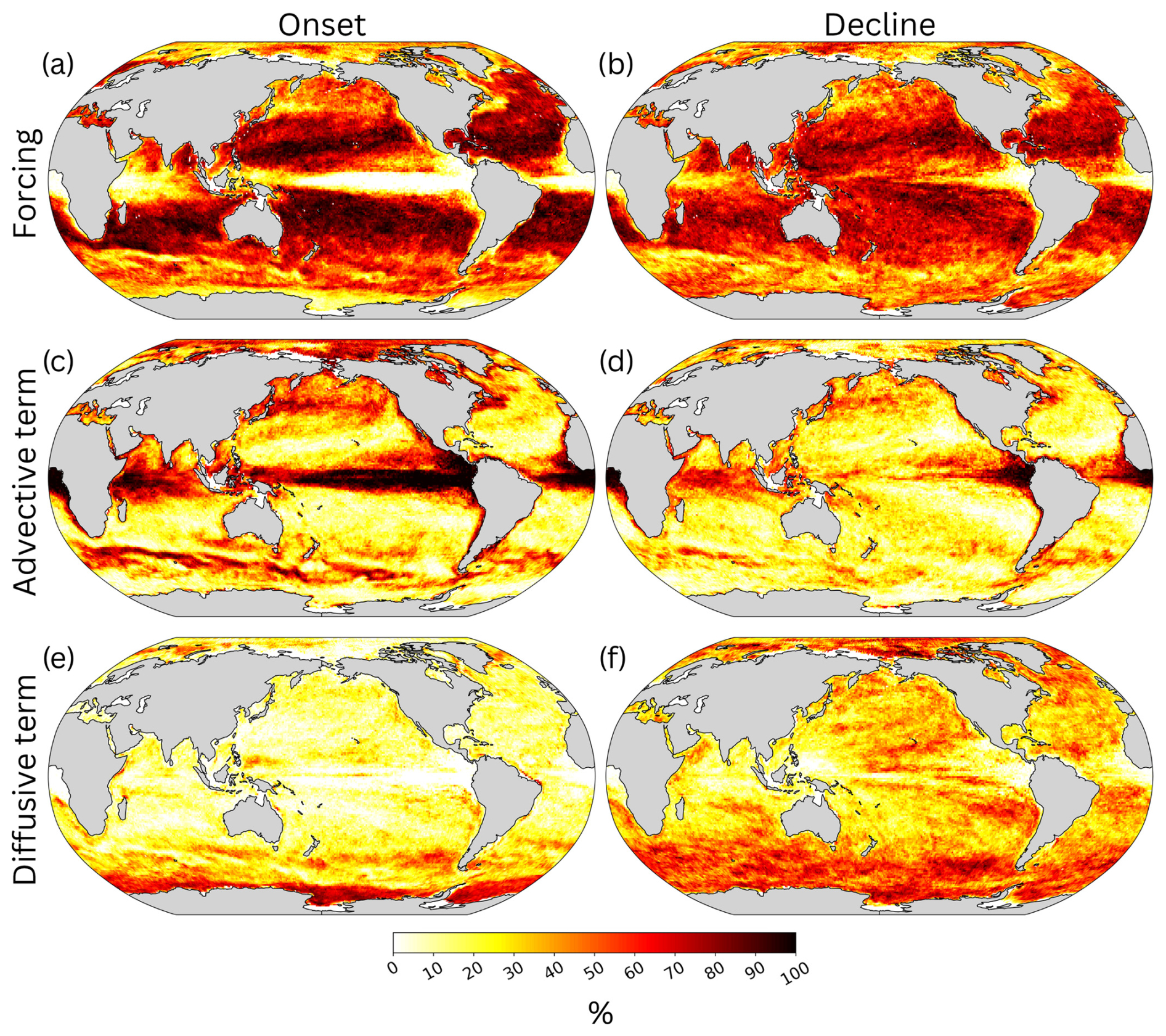
Figure 9 Same as Fig. 8 but for the percentage of times each term is a leading contributor to the MHW (a, c, e) onset and (b, d, f) decline phase. As an example, we include in the count in panel (a) for both a case in which atmospheric forcing is the only contributor to the onset phase and a case in which atmospheric forcing is a leading contributor along with the advective and/or diffusive convergence of heat.

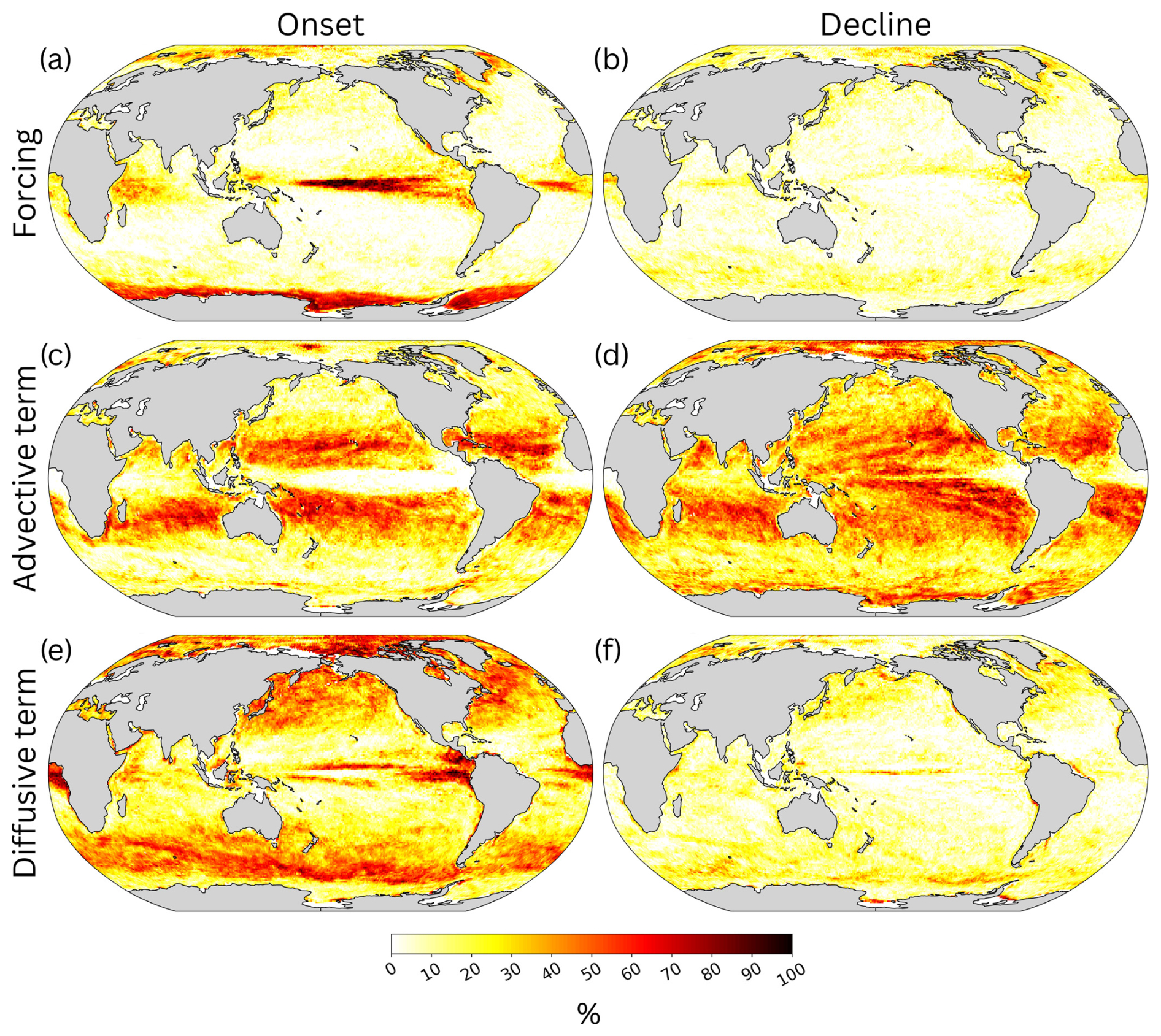
Figure 10 Same as Fig. 8 but for the percentage of times each term is the smallest contributor to the MHW (a, c, e) onset and (b, d, f) decline phase (regardless of how similar to other terms it may be).

4.3 Case studies in the Pacific Ocean

In the following, we discuss more details on the leading dynamical mechanisms of MHWs in three regions in the Pacific Ocean that have experienced at least one particularly intense MHW event: NEP, SWP, and TASMAN (introduced in Sect. 3.2 and shown as boxes in Fig. 1). While air–sea exchanges of heat play a key role in the onset and decline of most MHW events, there is diversity in the driving mechanisms of the two phases, both across regions and across events within each of the three regions. In some cases, ocean advective and diffusive processes (convergence and divergence) dominate the heat budget, emerging as leading contributors to MHW onset or decline.

During the time period analyzed here, 20 MHW events are observed in the NEP region, with 5 of them related to the northeastern Pacific marine heatwave of 2013–2016, also known as “the Blob” (events 15–19 in Figs. 11a and S2). The Blob was characterized by an extensive area of anomalously warm sea surface temperatures. It developed due to decreased surface cooling and reduced Ekman transport of colder water from the north, driven by persistent high-pressure systems in the region (Bond et al., 2015; Hartmann, 2015; Di Lorenzo and Mantua, 2016). This event was further sustained by ENSO-related Pacific climate variability through atmospheric teleconnections, which played a critical role in prolonging its duration and amplifying its impacts (Capotondi et al., 2022; Ren et al., 2023; Xu et al., 2022). Consistent with previous studies, events 15–18 in Fig. 11a show the leading contribution of atmospheric forcing to the onset phase, with additional contributions, in some cases substantial (e.g., events 16 and 17), from the advective or diffusive convergence of heat. Furthermore, the advective convergence of heat is the key driver of the onset of MHW Event 19 (Fig. 11a), highlighting the importance of multiple mechanisms working together to sustain MHW intensity and prolong its duration. The Blob also showed how changes in atmosphere–ocean interactions in response to initial SST anomalies (including a reduction in low-cloud cover enhancing insolation) may further sustain and intensify these anomalies, increasing their persistence (Myers et al., 2018; Schmeisser et al., 2019).

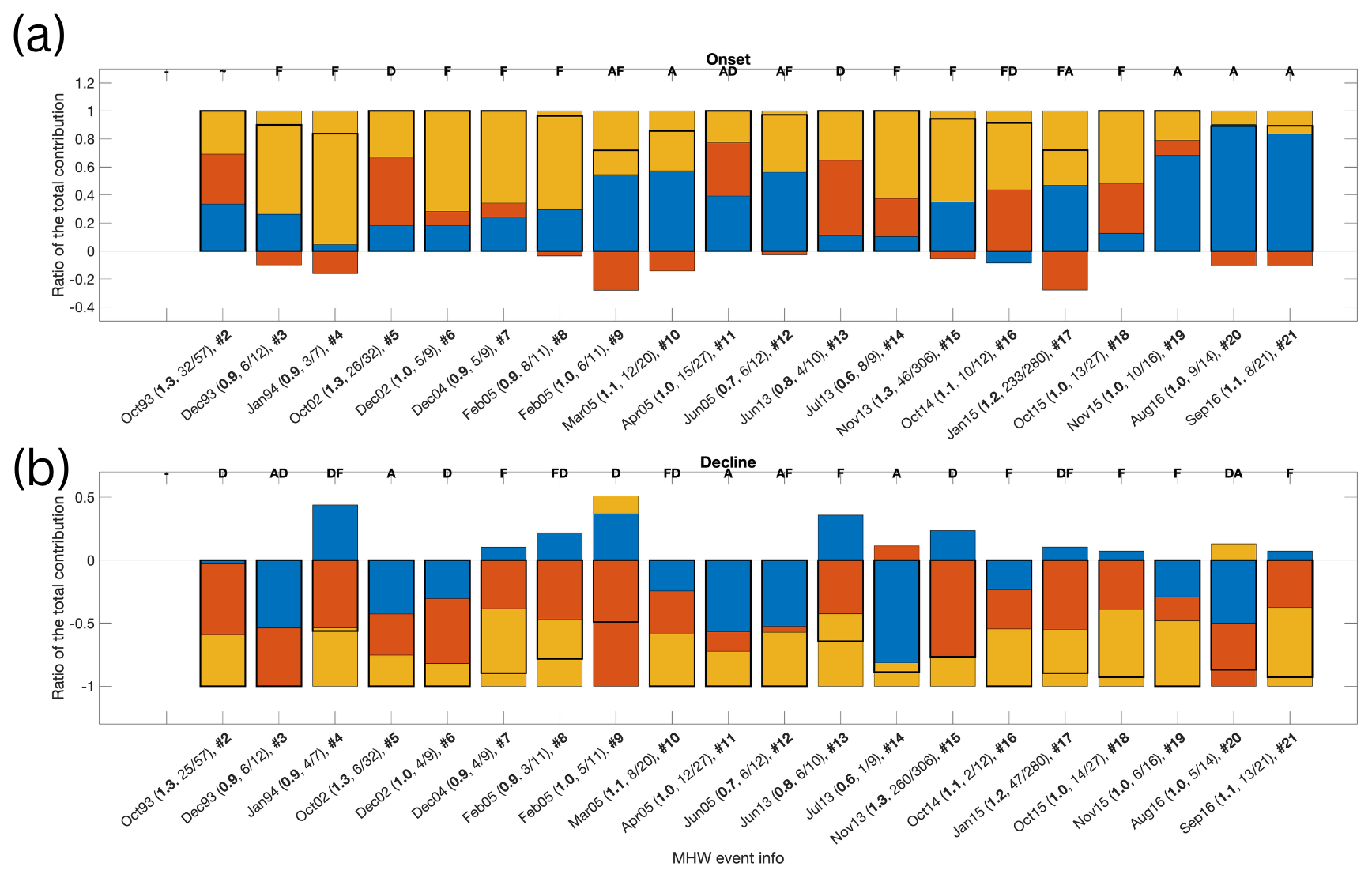
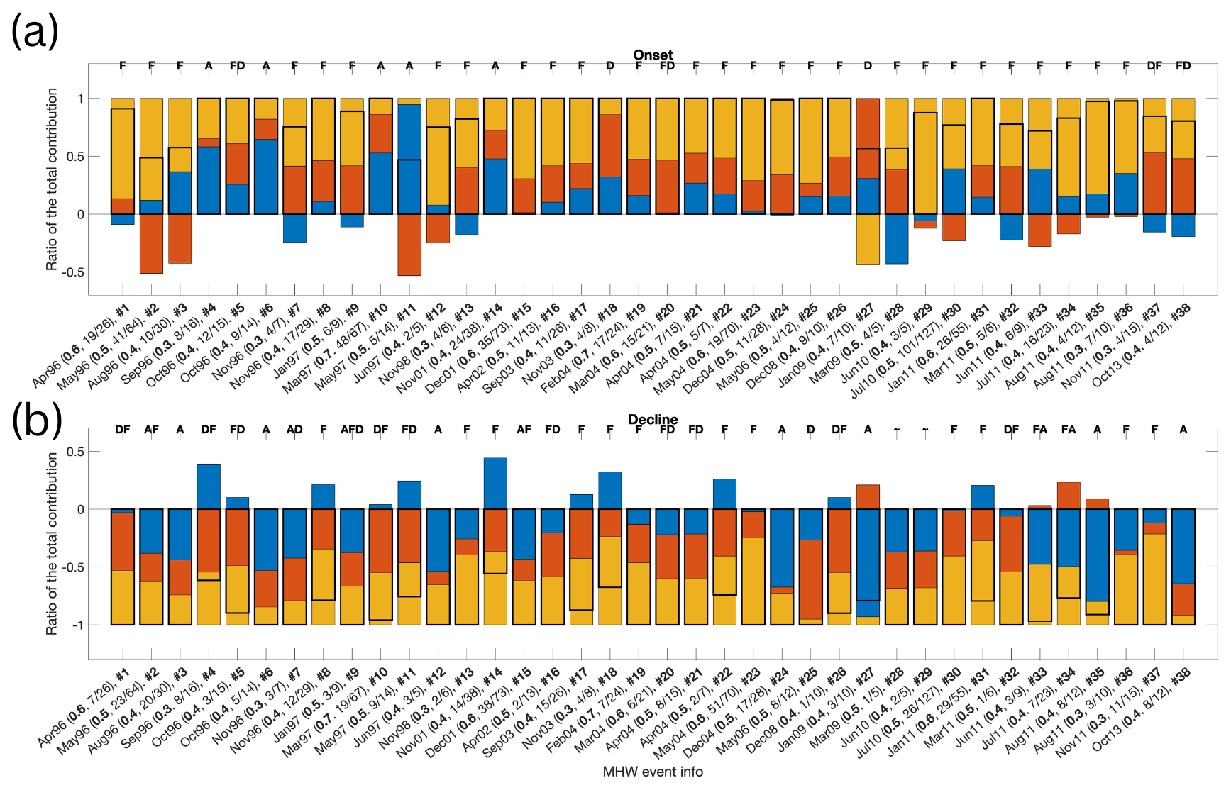
Figure 11 MHW events in the northeastern Pacific (NEP, region 1 in Fig. 1) based on the ECCOv4r4 upper-ocean (5–55 m) heat content: ratio of the total contribution for each budget term during each phase (onset/decline), as well as the tendency (also scaled by the total contribution). Panel (a) shows the onset phase, whereas panel (b) shows the decline phase. Each stacked bar represents the relative contribution of each term during that phase, with the total contribution (i.e., the sum of the terms that contribute to that phase) normalized to 1. The black outline over each bar indicates the total temperature tendency during that phase (scaled by the total contribution to that phase), showing agreement with the sum of the individual terms and confirming budget closure. The x-axis labels denote the start date of each MHW event, followed by values in parentheses indicating the event intensity (as average temperature (°C) in the layer used for the OHC estimate), onset/decline duration (in days), and total duration. The letter codes above each bar indicate which term(s) dominated the total temperature tendency during that phase (A – advection; D – diffusion; F – forcing). For example, “F” is used for cases in which the forcing provides the leading contribution; “FA” is used when both forcing and advective convergence provide a leading contribution; “AFD” characterizes cases in which advective convergence is larger than forcing and diffusive convergence and forcing are larger than diffusive convergence, yet the difference does not meet the 30 % criterion as in the previous two cases; and, finally, “∼” corresponds to cases in which all terms contribute comparably.

Overall, in the NEP region, atmospheric forcing is a key driver of MHW onset, leading the onset phase (alone or along with other processes) in about 50 %–70 % of cases (see tags that include “F” in Fig. 11a; also, see the sum of the percentages for “F” in the NEP onset column of Table 1) and being “the” leading process in about 40 %–45 % of the events (see tags with only “F” in Fig. 11a; e.g., Event 3). Heat transport by ocean currents is another key process during MHW onset, leading this phase (alone or along with other processes) in 30 %–50 % of cases and being “the” leading mechanism in four events (events 10, 19, 20, and 21 in Fig. 11a). While diffusive convergence of heat is “the” leading mechanism for MHW onset in the NEP in the time period of interest in just two instances (events 5 and 13 in Fig. 11a), it contributes along with air–sea exchanges and/or advective convergence in 5 %–10 % of cases, i.e., events 11 and 16 in Fig. 11a. Furthermore, the diffusive divergence of heat leads MHW decline (alone or along with other processes) in 45 %–55 % of the events; e.g., see the tags including “D” in Fig. 11b. In two of these events, the diffusive divergence of heat leads the decline phase along with the advective divergence of heat (“DA” and “AD” tags); in four events, diffusive divergence is “a” leading mechanism along with atmospheric forcing (see “DF” or “FD” tags in Fig. 11b). Overall, atmospheric forcing leads (alone or along with other processes) MHW decline in the region in about 45 %–65 % of the events (see tags including “F” in Fig. 11b, except if the tag has three letters and “F” is the last one) and is “the” leading process in six events (e.g., events 7, 13, 16, 18, 19, and 21). The advective divergence of heat is “the” leading mechanism in three events instead (events 5, 11, and 14) and is “a” leading process in 15 % of cases (along with forcing and/or diffusive divergence of heat). This is consistent with a diversity of leading dynamical mechanisms for MHWs in the NEP, both during onset and decline (Table 1).

Table 1 How often each budget terms is “the” leading term vs. “a” leading term (excluding overlap with “the”) across the NEP, SWP, and TASMAN regions.

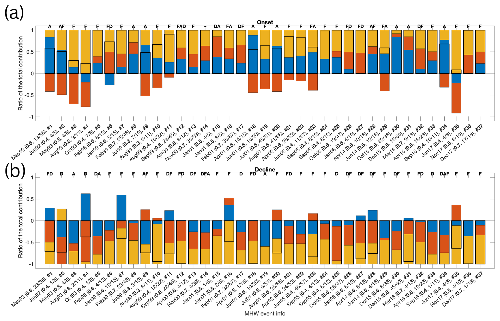
Diversity of leading mechanisms also emerges across the 38 MHW events in the SWP region (Table 1). In this region, extreme extratropical MHWs appear to be associated with different phases of the El Niño–Southern Oscillation (Dutheil et al., 2024; Gregory et al., 2024a). Indeed, MHW conditions were detected during the 2010–2011 La Niña event (Boening et al., 2012), corresponding to event 30 in Figs. 12 and S4c and d. The onset phase of this event was primarily driven by atmospheric forcing, consistent with about 71 % of SWP MHWs (e.g., see events 2, 12, 29, and 30 with tags “F” in Fig. 12a). This agrees with previous studies indicating that air–sea exchanges often dominate MHW development in the region (Sen Gupta et al., 2020). We also note that, in an additional 11 % of events, atmospheric forcing is a leading term during the onset along with advection and/or diffusion (e.g., events 5, 20, and 37 in Fig. 12a). Heat transport by ocean currents, i.e., the advective convergence of heat, is “the” leading process of SWP MHW onset in 13 % of events (events 4, 6, 10, 11, and 14 in Fig. 12a), while diffusive convergence of heat is “the” leading mechanism in only two cases (e.g., events 18 and 27 in Fig. 12a) and contributes alongside forcing and/or advection in about 11 % of cases (e.g., events 20 and 37 in Fig. 12a). As for the onset, atmospheric forcing leads MHW decline (alone or along with other processes) in most cases (about 66 %–71 % of the events; e.g., Event 30 in Figs. 12b and S4c). Atmospheric forcing leads MHW decline along with the diffusive divergence of heat in about 26 % of the events (e.g., Event 11 in Figs. 12b and S4b) and with advective convergence in about 11 % of the events (e.g., events 33 and 34 in Fig. 12b). Moreover, the advective divergence of heat is “the” leading term for MHW decline in 18 % of the events (e.g., Event 35 in Figs. 12b and S4f) and contributes alongside forcing and/or diffusion in another 13 % of events (e.g., Event 15 in Fig. 12b). Diffusive divergence of heat is “the” leading mechanism in only one MHW decline case (e.g., Event 25 in Fig. 12b), yet it is “a” leading term alongside other processes in 29 %–32 % of cases (e.g., events 5 and 11 in Fig. 12b).

Figure 12 Same as Fig. 11 but for the southwestern Pacific region (SWP, region 2 in Fig. 1).

Finally, 37 MHW events are found in the TASMAN region, where we again see a diversity of driving mechanisms (Table 1). Five of the events (events 30–34 in Figs. 13 and S5k–r) are associated with the intense 2015–2016 Tasman Sea marine heatwave described in Oliver et al. (2017). This unprecedented warming event, characterized by sustained heat anomalies, was attributed to the anomalous convergence of heat linked to the intensification of the southward-flowing East Australian Current (Kajtar et al., 2022), making it the longest and most intense MHW on record in the region (Oliver et al., 2017). Our results confirm that the advective convergence of heat is a primary driver during the onset phase of events 30, 31, and 34 (in Figs. 13a and S5k and o). More generally, the advective convergence of heat is “a” leading process (alongside other mechanisms) in 14 %–19 % of onset cases and “the” leading process in 22 % of events (e.g., events 1, 18, and 34 in Fig. 13a). Overall, as for the NEP and SWP, atmospheric forcing provides a key contribution to MHW onset in the TASMAN region in the majority of events (≈62 %–81 %), including about 38 %–49 % of events when it is “the” primary driver of the MHW onset (see tags with only “F” in Fig. 13a; e.g., events 3, 4, 11, and 35 in Figs. 13a and S5). This anomalous atmospheric forcing may originate from a variety of remote influences, associated with various modes of variability (e.g., ENSO, Indian Ocean Dipole, or Southern Annual Mode), as discussed in Gregory et al. (2023, 2024b), who used this information to inform MHW event predictability. Diffusive convergence of heat, while not being the only leading mechanism in any of the cases, is “a” leading process in about 11 %–19 % of the onset phases. In the TASMAN region, atmospheric forcing alone leads the decline phase in the region in around 38 %–41 % of events (e.g., Event 31 in Figs. 13b and S5l). In two events, air–sea exchanges of heat act along with the advective divergence of heat as the main drivers of the decline phase (e.g., Event 9; Fig. 13b). Forcing and diffusive divergence of heat lead the MHW decline in about 30 % of the events instead (see tags with “FD” or “DF” in Fig. 13; e.g., Event 12 in Fig. S5d). Additional decline-phase cases include two primarily driven by the advective divergence of heat (e.g., Event 3 in Fig. 13b) and four led by the diffusive divergence of heat (e.g., Event 25 in Figs. 13 and S5h). Overall, the advective and diffusive divergence of heat are a leading term for MHW decline in 5 %–8 % and 32 %–35 % of events, respectively.

Figure 13 Same as Figs. 11 and 12 but for the Tasman Sea region (TASMAN, region 3 in Fig. 1).

5 Conclusions

In this study, we have conducted a comprehensive analysis of marine heatwaves using various observational and reanalysis datasets to understand their characteristics and the leading dynamical processes that drive their formation and decline. We validate the ECCO ocean reanalysis data against observational data from OISST and Argo floats: ECCO is generally consistent with observations and critical for precisely assessing the processes responsible for MHW onset and decline, although it tends to underestimate the number and intensity of MHW events, especially at the daily timescale, and overestimate their duration, as also found for other models (see Capotondi et al., 2024, for a review).

We explore the heat budget terms contributing to the time evolution of MHWs, focusing on atmospheric forcing, advective convergence, and diffusive convergence of heat. Our results indicate that atmospheric forcing is the dominant contributor to both the onset and decline phases of MHWs across most oceanic regions, with the exception of equatorial regions and some locations in the extratropics and in the Southern Ocean, where ocean dynamics plays a key role. The advective convergence and divergence of heat are leading dynamical mechanisms for MHWs near the Equator, especially in the Pacific (where extreme warming is closely related to ENSO variability), in the western boundary currents, and (for the onset phase) along the Antarctic Circumpolar Current. The diffusive convergence and divergence of heat most often lead MHW onset and decline phases, respectively, in many regions of the Southern Ocean, except where the advective term is “the” leading dynamical mechanism.

Our analysis of the northeastern Pacific, southwestern Pacific, and Tasman Sea regions highlights the complex interplay of oceanic and atmospheric processes driving MHWs, underscoring the need for regional-scale studies to capture the details of local dynamics for different events. While atmospheric forcing plays a key role in MHW onset and decline across the three regions, in most cases, diverse combinations of processes are at play across regions and across events in the same region. Furthermore, in the NEP and TASMAN regions, the advective convergence of heat is a leading term during MHW onset more often than diffusive convergence, while the opposite is true for the decline phase. In contrast, in the SWP region, the two processes are leading mechanisms almost equally as often, both during onset and decline,.

Our findings (1) highlight the importance of using daily data to study leading dynamical processes during MHW onset and decline and (2) emphasize the importance of comparing ocean state estimates and reanalyses with a suite of observations to better understand the strengths and limitations of these products. Understanding MHWs' leading dynamical processes and their regional variations is essential for predicting MHWs and assessing their potential impacts on marine ecosystems and global climate patterns. Future research should aim to further refine these analyses by incorporating more regional studies of MHWs in the present and future climate and exploring the interaction between physical processes and biological responses to MHWs.