Currents and their drivers in the Archipelago Sea: insights from ADCP measurements

The Archipelago Sea (AS) in the Baltic Sea is a complicated fragmented sea area with numerous small islands and islets that are crossed by several deeper straits. The area functions as a major route for both transport and leisure activities on the sea as well as many other forms of the blue economy. Even with the large number of maritime activities in this sea area, knowledge of the currents along the deep channels crossing the AS has been limited due to the lack of quality-assured measurements. To enhance the general understanding of the dynamics in the AS, we have collected and analysed currents in 10 different locations across the AS using acoustic Doppler current profiler (ADCP) current measurements made during numerous short measurement campaigns over the last two decades. Currents in the AS are restricted by the geometry of the area and typically have two main flow directions, with a slightly wider directional distribution at the southern parts of the AS. In open areas of the AS, surface currents have a mean magnitude of around 8 cm s⁻¹ and can momentarily grow to significant magnitudes, as even the shortest measurement time series (of around 4 months) have measured currents exceeding at least 40 cm s⁻¹. The current magnitudes in the long and narrow straits are almost double (14 cm s⁻¹) the general current magnitudes of the area, and current magnitudes up to 115 cm s⁻¹ have been measured at the northern end of the long northeastern strait. The AS currents are mostly driven by local winds, but strong oscillations in the surrounding basins can cause significant currents (up to 80 cm s⁻¹ in narrow straits) if the local winds are weak enough (below 10 m s⁻¹) or from non-optimal directions with respect to the straits. Our analysis shows that especially strong seiche in the Gulf of Finland combined with low sea levels in the Gulf of Bothnia is a significant factor in forcing currents in the AS.

1 Introduction

The Archipelago Sea (AS) is a unique and complicated coastal archipelago located in the Baltic Sea (Fig. 1). It is a region with over 40 000 small islands and islets, narrow channels between islands, and a large variation in bottom topography. Together with the Åland Sea, the AS separates the two major Baltic Sea basins with independent oscillation and circulation patterns: the Baltic proper together with the Gulf of Finland from the Gulf of Bothnia (Wubber and Krauss, 1979; Jönsson et al., 2008). The AS is also a heavily trafficked area with narrow fairways. In some of these fairways, there can be sudden strong currents (Kanarik et al., 2018), potentially causing dangerous situations for navigation when the flow direction is from the side of the vessel. For the safety of marine traffic, it is essential that different operators, e.g. pilots, have detailed knowledge of areas and situations in which such strong currents can occur. Thus, understanding the main features of currents in different areas of the archipelago and the drivers behind them is important. As currents also transport substances within the water column, understanding circulation dynamics provides knowledge-based information to support spatial planning for offshore activities such as aquaculture.

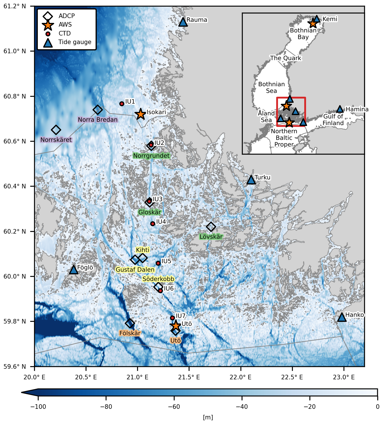
Figure 1 Locations of the current measurements (ADCP, acoustic Doppler current profiler) in the Archipelago Sea (AS), indicated with diamonds. The Fölskär and Utö measurement stations (names highlighted in orange) are located at the southern edge of the AS; Kihti, Gustaf Dalen, and Söderkobb (yellow) in the central AS; Norrgrundet, Gloskär, and Lövskär (green) in narrow straits; and Norrskäret and Norra Bredan (purple) at the northern edge of the AS (as presented in the corresponding Sect. 3.1 to 3.4). The stars and triangles indicate the locations of the automatic weather stations (AWSs) and tide gauges, respectively. Red dots indicate the location of the routine CTD (conductivity–temperature–depth) stations between Isokari and Utö. The background colour represents the bathymetry (EMODnet Bathymetry Consortium, 2020), and the grey lines indicate the borders of different sea basins. The smaller map shows the different basins in the northern Baltic Sea, and the red rectangle indicates the location of the study area. Basin borders and coastline from HELCOM (2018).

The first current measurements in the Baltic Sea were conducted more than a century ago using a large network of lightships, which were essentially floating lighthouses that were also utilised for marine observations (Witting, 1912; Palmén, 1930; Hela, 1952). Studies based on these measurements gave us information on the general circulation patterns of the Baltic Sea and showed that the currents, especially in the surface layer, are strongly dependent on the wind climate. The general Baltic Sea wind fields are characterised by dominant southwesterly (SW) and secondary north-northwesterly (NNW) winds (Soomere and Keevallik, 2001; Männikus et al., 2020), as shown also in the AS area (Miettunen et al., 2024). The Baltic Sea is located at the end of the North Atlantic storm track and has large seasonal variability in the occurrence of windstorms, with the most frequent occurrences between November and January and the least between May and August (Laurila et al., 2021a), while also experiencing large annual and decadal variability (Laurila et al., 2021b). These variations in wind and atmospheric pressure are also the main factors affecting short-term sea level variations in the Baltic Sea (Johansson, 2014). Recent studies have also been able to further identify that most extreme sea level events in the Baltic Sea are related to events with clusters of cyclones crossing the Baltic Sea region in a short period of time (Rantanen et al., 2024).

Today, observation-based studies of the circulation in the Baltic Sea are rather rare and have mainly focused on certain areas as part of temporary moorings utilising acoustic Doppler current profiles (ADCPs) (e.g. Muchowski et al., 2023; Green et al., 2006). Several studies have recently focused on the Gulf of Finland, where the analysis of measured currents has shown that while currents are mainly driven by wind and bathymetry, seiche and tides can play a significant role in the area's circulation dynamics (Lilover et al., 2011). In the Gulf of Finland, current oscillations have been shown to be strongly aligned with seiche modes in different parts of the water column depending on the prevailing stratification (Suhhova et al., 2018). Seiche oscillation is a specific feature of the semi-enclosed Baltic Sea sea level variations. It typically forms when wind and air pressure induce strong sea level gradients between different sub-basins (e.g. Gulf of Finland – Baltic proper). After the atmospheric forcing ceases, the strong gradient between basins can result in an oscillation of water back and forth between the sub-basins. The periods of these oscillations range up to 27 h between the Baltic proper and the Gulf of Finland and up to 39 h between the Baltic proper and the Gulf of Bothnia (Lisitzin, 1974; Wubber and Krauss, 1979). The tides in the Baltic Sea are usually on the order of a few centimetres (e.g. Witting, 1908, 1911). The strongest tidal oscillations have been observed in the Gulf of Finland, with amplitudes of 17–19 cm (Medvedev et al., 2013), and are clearly distinguishable in the current spectrum (Lilover, 2012).

In the AS, the first current measurements were made in 1922 as part of a study related to water exchange studies between the Baltic proper and the Bothnian Sea (Witting, 1925; Lisitzin, 1951). Measurements made near the surface and at 20 m depth showed a strong steering of the currents due to the bathymetry and geometry of the islands. In 1977, current measurements were made at three locations in the Archipelago Sea (Ambjörn and Gidhagen, 1979). Those records included a strong northward current of 91 cm s⁻¹ at one of the measurement locations at the narrow south-northward strait, while the maximums at the two other locations were around 50 cm s⁻¹. During the years 1974–1977, a large measurement campaign was carried out in the inner part (closer to the mainland) of the AS (Virtaustutkimuksen neuvottelukunta, 1979) with the aim of evaluating the fate of substances released from wastewater sources. Measurements were made at 15 locations and showed that currents in the inner and mid-archipelago have short-term fluctuations between two main directions. The current magnitude was weak on average, but occasionally there were high magnitudes. The highest measured current magnitude was ca. 50 cm s⁻¹. In 2004 and 2006 and from 2016 onwards, more recent current measurement campaigns have been conducted in the outer regions of the Archipelago Sea using ADCPs; however, they have not been made public nor published as of the writing of this paper.

Earlier research on AS currents has focused mainly on the effect of the wind and the geometry of the area to explain the drivers of the current fields. Virtaustutkimuksen neuvottelukunta (1979) evaluated the effect of winds on currents in the inner parts of the AS and concluded that the interactions are highly complicated due to the heterogeneity of the area. They found that the connection between wind direction and current direction was clearest when the winds were aligned along the channels and blowing from the same direction for longer periods. A model study, focussing on the more open areas of the AS, has shown that due to the geometry of the archipelago and the orientation of the channels, the southward transports were the largest with NNW winds and the northward transports with SSE–SE winds (Miettunen et al., 2020). The prevailing wind direction in the area, i.e. SW, is not optimal for northward or southward flow through the archipelago. This was also demonstrated by the analysis of current measurements in the Lövskär cross section, where currents were shown to be very sensitive to even small changes in wind directions and where even 15 m s⁻¹ SW winds were not able to induce strong currents in that cross section (Kanarik et al., 2018). Recent modelling studies have shown that there is large spatial and year-to-year variability in current speeds and directions in the Archipelago Sea (Tuomi et al., 2018; Miettunen et al., 2020, 2024). The model results show that in the deep, narrow channels that cross the area in the N–S or NW–SE direction, the current speeds are highest, and the directions are strongly aligned along the axis of the channels. In more open areas, the directional distribution of currents is wider, and the currents are weaker.

We publish ADCP datasets from the Archipelago Sea area and describe the general features of the measured currents. In our analysis, we considered the heterogeneity in the temporal and spatial coverage of the datasets. Using some of the longer datasets, we examined the drivers of the strong currents in the AS, which were left unexplained in earlier research that focused mainly on the local wind conditions (Virtaustutkimuksen neuvottelukunta, 1979; Kanarik et al., 2018). This was done by also considering the differences in sea level and atmospheric pressure over the AS.

2 Materials and methods

2.1 Current measurements

In this paper, we present and analyse only current measurements that are done with ADCP current profilers. We have data from 10 different locations around the Archipelago Sea (Table 1, Fig. 1). Measurements were done using a bottom-mounted Teledyne RD Instruments 300 kHz WORKHORSE Sentinel Broadband Acoustic Doppler Current Profiler. Data were quality checked using internal quality parameters (signal correlation, echo intensity, percent good, and error velocity) based on recommendations by Book et al. (2007) and Symonds (2006). For more detailed information on the exact procedure and the threshold values used, see Kanarik et al. (2018, Sect. 3). In the following analysis, we used only data quality flagged as 1 (good data). Bad quality data were marked as NaN in the analysis, thus leaving data from unmeasured areas completely out of the analysis. Datasets that have a large amount of missing data are marked in the figures to highlight the higher uncertainty of the given values.

Table 1 ADCP (acoustic Doppler current profiler) moorings used in this study. The given depth is the depth measured during the deployment of the ADCP. Stations with multiple deployments in the same location are indicated with a “–” in the “Name” column. The “Area” column identifies the type of the region (see Sect. 3) where the measurements were conducted.

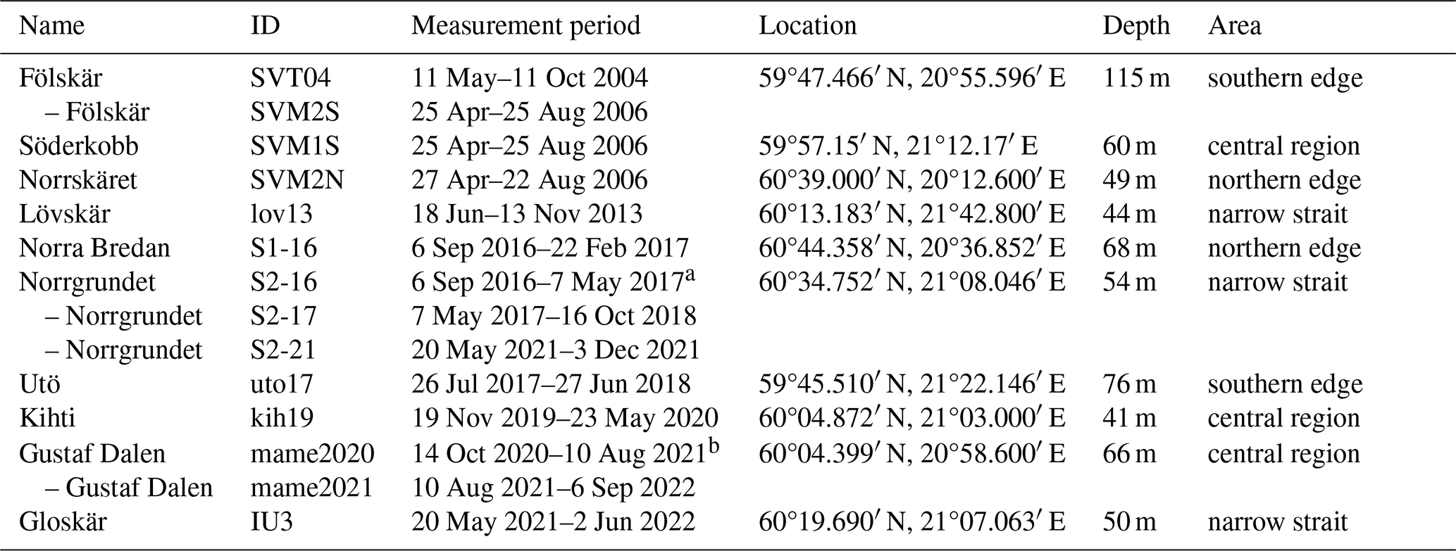
^a Device replaced on 7 May 2017. ^b Device replaced on 10 August 2021.

Table 2 Quality information about the ADCP measurements, presented in the same order as in Table 1.

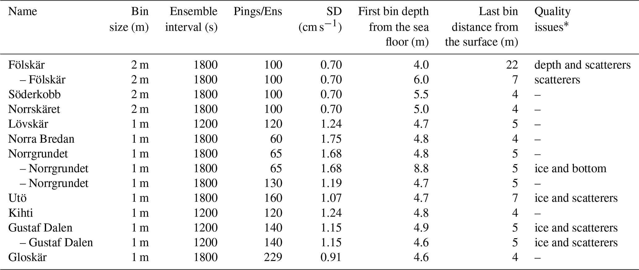
^* Check Sect. “Quality issues” under Sect. 2.1 for a more precise description of the quality issues.

The amount of subsurface bins that were rejected due to side slope contamination varied between the measurement stations and are presented in Table 2 together with information about the depth of the first measured bin, bin size, ensemble interval, number of pings per ensemble, and corresponding standard deviation (SD) of the measurements. As the sea surface variations in the Archipelago Sea (AS) are small, typically less than the bin size of the measurements, one depth level was used for flagging the data for side slope contamination for each time series (cf. “Last bin distance from the surface”, Table 2). ADCP was set to reach the sea surface in all but one dataset, i.e. the Fölskär measurements from 2004, in which the topmost bin was at 22 m depth. In the used configurations, we lost data from the approximately 5 m boundary layers at the sea surface and at the sea floor. Magnetic variation was corrected by calibrating compasses prior to deployments and applying up-to-date magnetic declination correction.

Quality issues

At some measurement sites and periods, there was loss of data due to physical or biogeochemical conditions (e.g. ice cover or lack of scatterers). These are marked as “Quality issues” in Table 2. The amount of good data for the whole water column for each station is presented monthly in Fig. 2, where the values indicate the fraction of good data for the whole month from all of the measured depths. If measurements started or ended in the middle of the month, then only the fraction of the measured month is marked as good. For example, measurements at the Kihti station started on 19 November, and there were no major issues in the measurements, so the measurements covered about 40 % of that month.

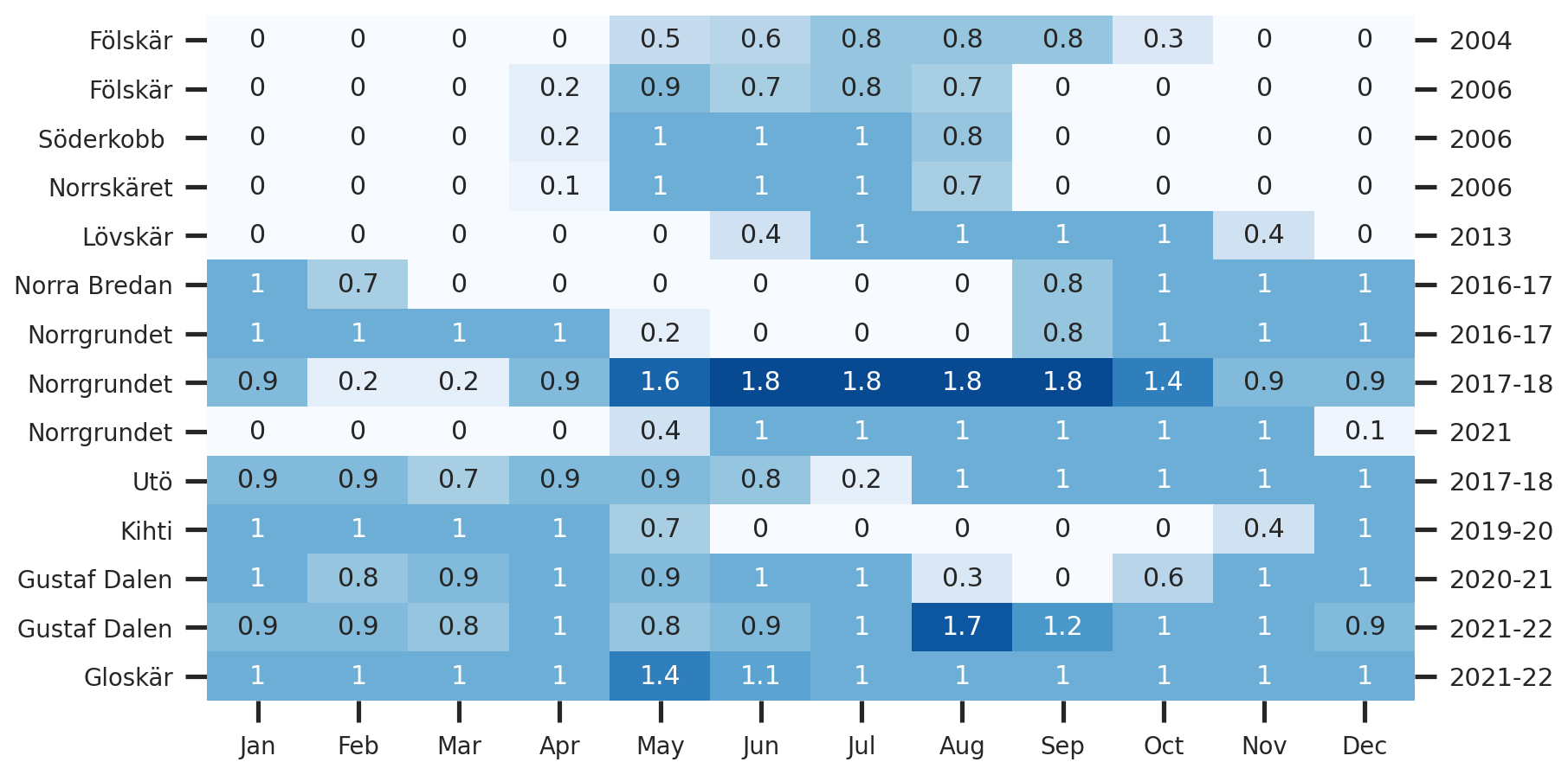
Figure 2 Amount of good data available throughout the whole water column per month for each measurement dataset (Table 1). The years of the measurements are shown on the right-hand-side y axis. A value of 1 indicates that the data were good throughout the water column for a whole month and that currents were measured at this location only during one year. Values greater than 1 indicate that the measurements spanned the next year. See Table 1 for the exact measurement periods.

The ice cover affected the measurement quality in February and March 2019, 2021, and 2022 (Fig. 2). The effects of ice were notable in February–March 2018 in Norrgrundet, in March 2018 in Utö, and in Gustaf Dalen during two winters: February–March 2021 and December 2021–March 2022 (Fig. 2). At the Utö and Gustaf Dalen sites, ice affected the measurements mainly only in the upper half of the water layer. However, in Norrgrundet, the ice corrupted the measurements in the entire water column, and the data were discarded for the whole time period from 6 February to 22 March 2018. During March 2018, most of the measurements at the Utö station were also of bad quality.

The lack of scatterers in spring and early summer also caused reoccurring quality issues in the ADCP data. Because of this, the ADCP did not receive enough valid signals from certain depths of the water column, typically around pycnocline. At Gustaf Dalen, ADCP was unable to measure currents around 10–20 m depths during May 2021 (Fig. 2). Data were also missing at the Utö station at the beginning of June 2018 at depths of 10–24 m and in the topmost 10 m layer in the last half of June. In some areas, measurements were successful during the night, when zooplankton migrate to the surface. An example of this lack of data in parts of the water column can be seen in Westerlund et al. (2022, Fig. 4). Zooplankton movement also caused some minor issues, e.g. in the thermocline in the Lövskär dataset (Kanarik et al., 2018), but only a nominal part of the data had to be rejected.

The depth of the Fölskär site (115 m) was too deep for the 300 kHz ADCP, as the device was mostly unable to acquire measurements in the upper 50–60 m of the water column. In the first dataset (measured in 2004), the maximum number of measurements was missed at depths of 36–38 m, where ADCP was unable to compute the current velocities from 68 % of the measured times. The next measurement campaign in 2006 was only slightly more successful, with the maximum amount of missing data being 53 % at 36–38 m depths. The lack of scatterers also contributed to the amount of missing data at this site. Data were missing most frequently between June and July in both years. Measurements close to the surface (7 m depth, Table 2) were only obtained in 2006 from mid-June onwards. Together, of the two measurement campaigns in Fölskär, only 35 % of the measurements were successful at the near-surface layer above the seasonal thermocline. However, there were almost no missing data in either of the measurements below 60 m down to almost 110 m in depth.

In the second Norrgrundet dataset (ID S2-17, Table 1), vertical velocities and thus error velocities were exceptionally high at the four bottommost bins. The error velocity tests rejected 21 % of the data from these depths, but because the vertical velocities still had unrealistic data after these automatic quality checks, we rejected all measurements from the four bottommost depth bins in this dataset.

2.2 Wind, sea level, and hydrography data

We used wind data from two automated weather stations (AWSs) to represent weather conditions in the surrounding seas. The Utö AWS (59°46^′44.74^′′ N 21°22^′29.24^′′ E) is located on the southernmost island of the AS, and the Isokari AWS (60°43^′19.91^′′ N, 21°1^′36.52^′′ E), at the northeast edge of the AS (locations shown in Fig. 1). Easterly, southerly, and westerly winds (measured at 25 m above mean sea level) at the Utö AWS represent the conditions in the northern Baltic proper, but northerly winds are affected by the northern islands and NW peninsulas of Utö island. The Isokari AWS has open sea from SW to N, and the winds are measured at 31 m above mean sea level. As wind measurements are made on the eastern edge of the Isokari island, the size and shape of the island weaken the winds from the western sector between the S and NNE directions; however, winds from the E are slightly overestimated due to the height of the measurement device. For analysis of larger-scale atmospheric conditions, atmospheric pressure measurements from the Kemi lighthouse AWS (65°23^′6.28^′′ N, 24°5^′44.46^′′ E, Fig. 1) were used together with the Utö AWS measurements.

For statistical analysis of general wind conditions over the AS, we used the climatological standard normal period of 1991 to 2020. For the first decade, data were available only once every 3 h. Because of this, statistical analysis over the given 30-year period was done using the same time interval of 3 h. The highest available temporal resolution was used when the winds were analysed against simultaneous current measurements. Measurements with 10 min intervals were available at the Utö AWS starting from 13 September 2006 and at the Isokari AWS from 2 May 2006. Continuous simultaneous data of atmospheric pressure from multiple AWS stations were available only from 2007 onwards, and the statistical analysis on this variable was thus conducted over a shorter time period.

To evaluate the relation between currents and the sea level differences over the area, we analysed instantaneous sea level data from tide gauges at Rauma (61°8^′2.03^′′ N, 21°26^′33.47^′′ E), Hanko (59°49^′22.32^′′ N, 22°58^′35.70^′′ E), Turku (60°25^′41.81^′′ N, 22°6^′1.92^′′ E), Föglö Degerby (60°1^′54.78^′′ N, 20°23^′5.34^′′ E), Hamina (60°33^′45.96^′′ N, 27°10^′45.12^′′ E), and Kemi (65°40^′24.13^′′ N, 24°30^′54.94^′′ E). The locations are marked in Fig. 1 with triangles. The sea level values used are given relative to the theoretical mean sea level. For statistical analysis of typical sea level difference, we used hourly instantaneous data over the climatological standard normal period of 1991 to 2020.

Wind and sea level measurements are publicly available in the open database of the Finnish Meteorological Institute (FMI; https://en.ilmatieteenlaitos.fi/open-data, last access: 27 February 2025).

Temperature and salinity profiles were collected from seven stations located along a north–south transect across the Archipelago Sea from Isokari to Utö (Fig. 1, IU locations). Data were analysed for the years 1991 to 2021, during which the total number of profiles measured at each station varied between 35 and 66. These data are available through https://www.marinefinland.fi/en-US (last access: 6 June 2024) or through the ICES data system (https://www.ices.dk, last access: 6 June 2024).

2.3 Calculation of persistency (P)

The variability of the current direction was described using the persistency value (P) as defined by Witting (1912) and Palmén (1930):

$$\begin{array}{}\text{(1)}& P={\displaystyle \frac{\sqrt{(\frac{\mathrm{1}}{N}{\sum }_n{u}_n{)}^{\mathrm{2}}+(\frac{\mathrm{1}}{N}{\sum }_n{v}_n{)}^{\mathrm{2}}}}{\frac{\mathrm{1}}{N}{\sum }_n\sqrt{u_n^{\mathrm{2}}+v_n^{\mathrm{2}}}}}\times \mathrm{100},\end{array}$$

where u_n and v_n are the eastward and northward components of the current velocity at time step n. N stands for the total number of observations in the time series, n indexes each observation from 1 to N, and ∑ denotes the sum over all time steps from n=1 to N. Currents that are unidirectional in time have a persistency of 100 %.

3 General characteristics of the Archipelago Sea currents

Due to the temporal and spatial heterogeneity of the dataset, we divided it according to geographical location and season. Geographically, we used four areas: (1) the southernmost part of the AS, which has been shown to have a wider directional distribution and lower current magnitudes than the other areas (e.g. Miettunen et al., 2024); (2) central open areas of the AS; (3) narrow straits with fairways (e.g. Kanarik et al., 2018); and (4) northern areas, which are geographically located at the Bothnian Sea but have connection to the AS through the narrow straits crossing the northern part of the AS.

The distribution by season was done based on the variation in hydrography, winds, and ice conditions. The seasonal thermocline is most prominent in July, August, and September, typically at depths of 15–20 m (Fig. 3). During other seasons, temperature and salinity are vertically mostly homogeneous. The extent of ice in the Archipelago Sea is typically highest in February and March. Wind conditions also show a large seasonal variation. Storms are frequent between October and March, while the warm season between April and September is typically calmer (Laurila et al., 2021a). Also, the wind direction has seasonal variation, e.g. NNW winds are more typical during warm seasons (Fig. 4). Based on these, we decided to use the following division into seasons: winter – January to March (JFM); spring – April to June (AMJ); summer – July to September (JAS); and autumn – October to December (OND).

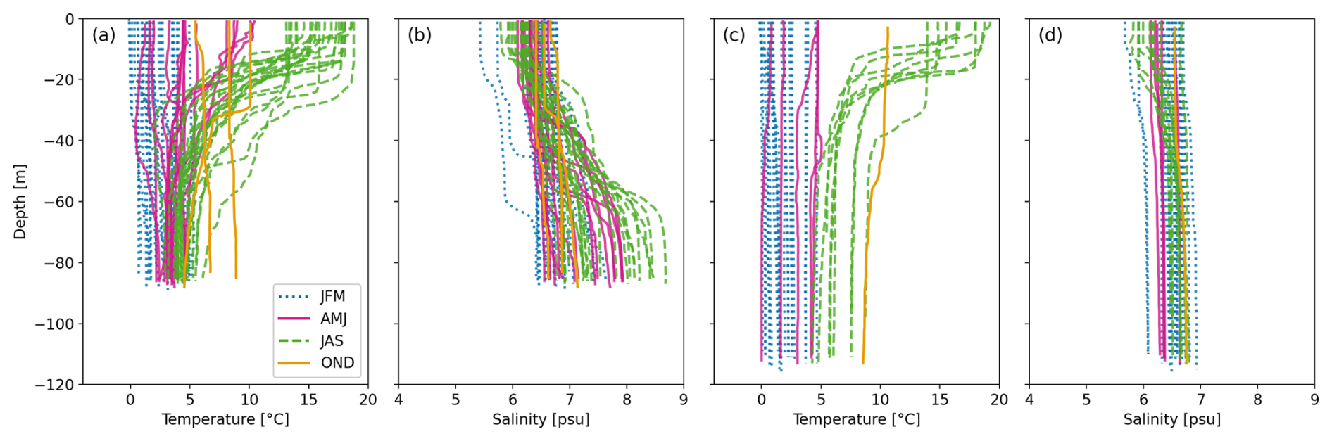
Figure 3 CTD profile measurements from 1991 to 2021 from IU7 (a, b) and IU6 (c, d) stations in the southern Archipelago Sea (locations marked in Fig. 1). There are a total of 67 profiles from IU7 and 35 profiles from IU6. Colours represent different seasons.

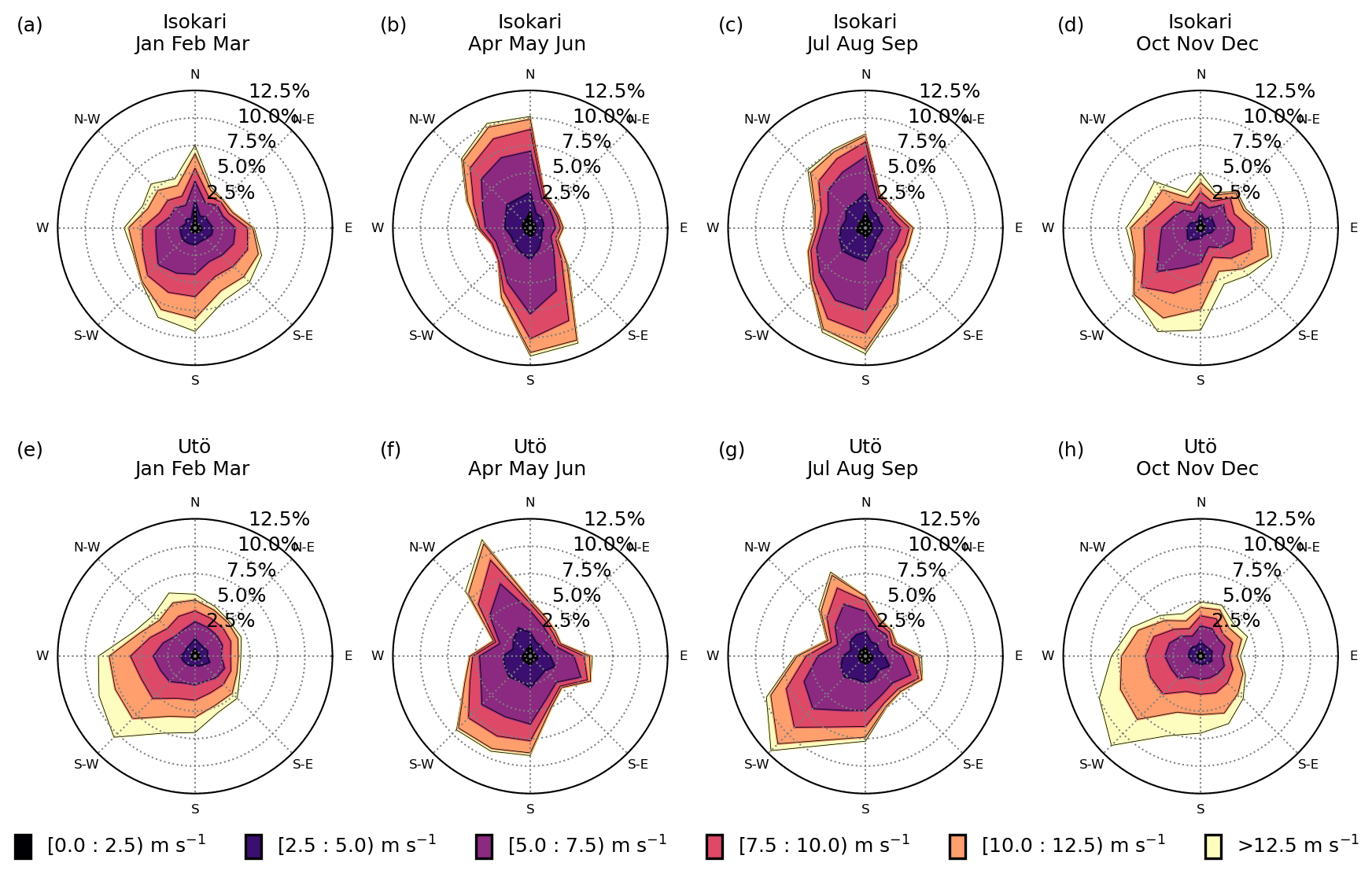
Figure 4 Winds in different seasons in Isokari (a–d) and Utö (e–h). Directions show where the wind is coming from.

3.1 Currents near the southern edge of the Archipelago Sea

The Utö and Fölskär measurements represent the southernmost AS, where the occasional halocline and seasonal thermocline divide the water into two or three layers (see station IU7 in Fig. 3), of which the topmost, i.e. surface layer, is directly affected by winds. The mean current magnitudes calculated from the entire water column were around 6–7 cm s⁻¹, with higher values measured at the Utö station than in Fölskär. The maximum magnitudes reached 58 cm s⁻¹ in Utö (surface layer) and 53 cm s⁻¹ in Fölskär (intermediate layer,¹ above the halocline). The halocline in this area has a large seasonal and interannual variation in its occurrence and depth, as shown, e.g., by Laakso et al. (2018). The presence of the halocline during our current measurement campaigns can be observed from the change in flow directions in different layers of the water column from the two southernmost stations.

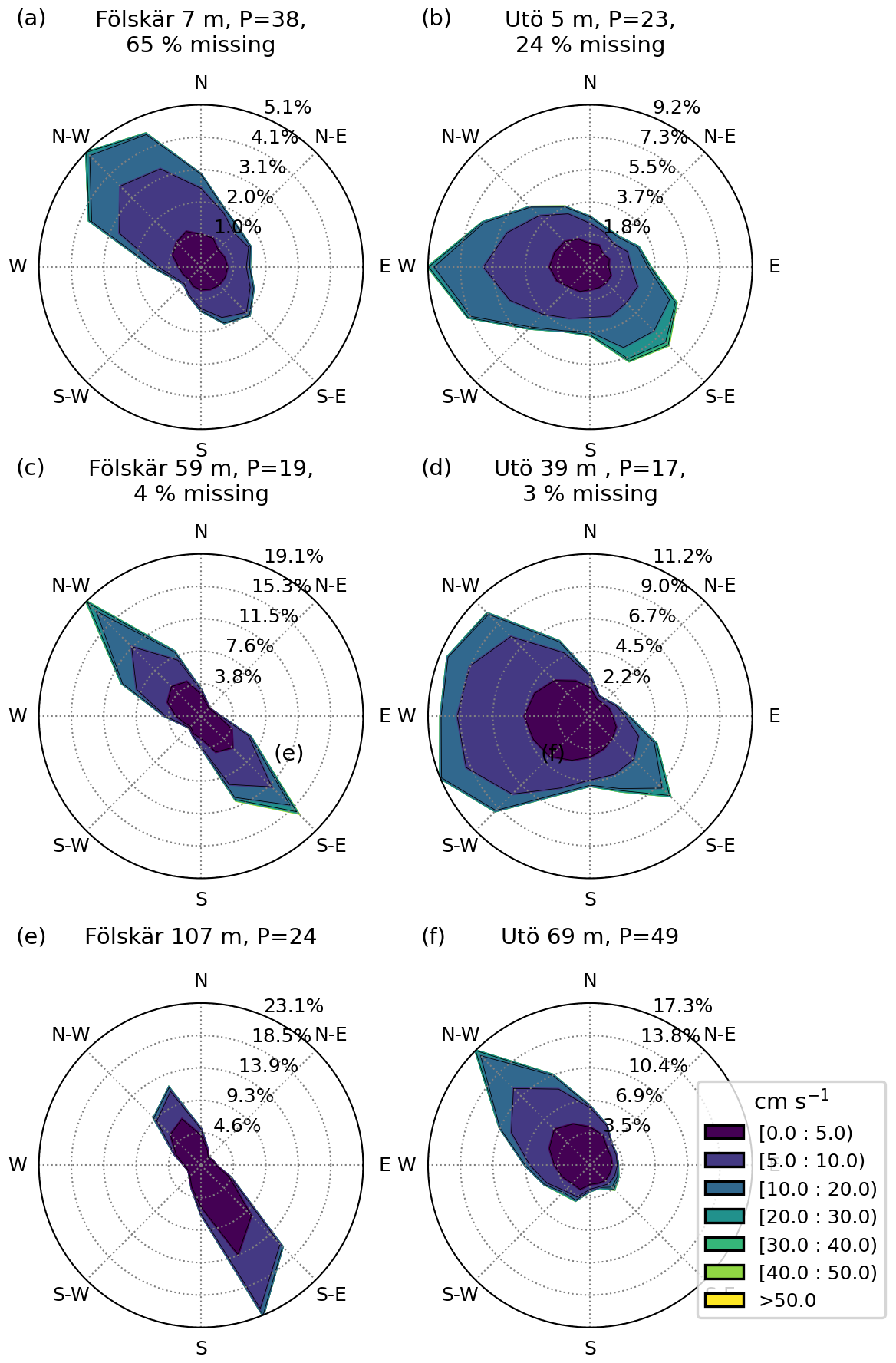
Figure 5 Current roses from the southern stations. Panels (a) and (b) show the measurements closest to the surface, panels (c) and (d) show currents on top of the halocline, and panels (e) and (f) show the measurements closest to the sea floor (station depths in Table 2), with the corresponding persistency (P, %). The percentage of missing data during the measurement period is shown for layers with a significant amount of missing data. Directions show where the current is flowing to. For further information on the missing data, see Sect. “Quality issues”.

The prominent current direction in the layer closest to the surface was towards the NW in the westernmost strait (Fölskär, Fig. 5) with a mean magnitude of 7 cm s⁻¹ and a persistency (P) of 38 % and towards the W at the easternmost station (Utö, Fig. 5) with a mean magnitude of 8 cm s⁻¹ and P of 23 %. At the bottommost layer, separated from the rest of the water column by the halocline, the flow was mostly steered by the bottom topography and directed towards the SSE (P of 24 %) at the Fölskär station and toward the NW at the Utö station, where the P was highest (49 %) in the area. The mean magnitudes at the bottom varied between 4 and 6 cm s⁻¹, with lower values measured in Fölskär. Even at the bottom, magnitudes up to 21 cm s⁻¹ (Fölskär) and 38 cm s⁻¹ (Utö) were measured.

The current directions in the intermediate layer, between the seasonal thermocline and the halocline, had a large spread and the lowest persistencies (P). At the Utö station, a large part of the currents were directed toward the W/WSW with P of 17 %. At the Fölskär station, flow in the intermediate layer was evenly distributed between the NW and SE with P of 19 %, whereas at the surface, the most frequent direction was towards the NW rather than the SE. It should be noted that the surface layer measurements were available only from the later Fölskär deployment (Table 1, ID SVM2S) from April to August, and even these had notable data gaps due to a lack of scatterers in the surface layer during the day. The short measurement period together with less available data at the layer above the seasonal thermocline largely explains the overall smaller current magnitudes at the Fölskär site, as elaborated in Sect. 3.5.

3.2 Currents in the central Archipelago Sea

Measurements in the central areas of the AS were made in three different locations: Gustaf Dalen, Söderkobb, and Kihti. This central region is relatively open compared to other areas of the AS. However, the area is considerably more open in the NW–SE direction than in the SW–NE direction, as there are small islets on both sides of the deep straits crossing the region. Due to this geometry, the main flow direction of the currents at the surface is also toward the NW or SE (Fig. 6, upper panels). The persistency at the surface layer was lowest at Gustaf Dalen (P of 16 %), located at the crossing of the two deeper straits (Fig. 1), and about twice the value in the surrounding Sörderkobb (P of 38 %) and Kihti (P of 33 %) measurement stations. The magnitudes in the surface layer varied between 8 and 9 cm s⁻¹, with a higher value measured in Kihti.

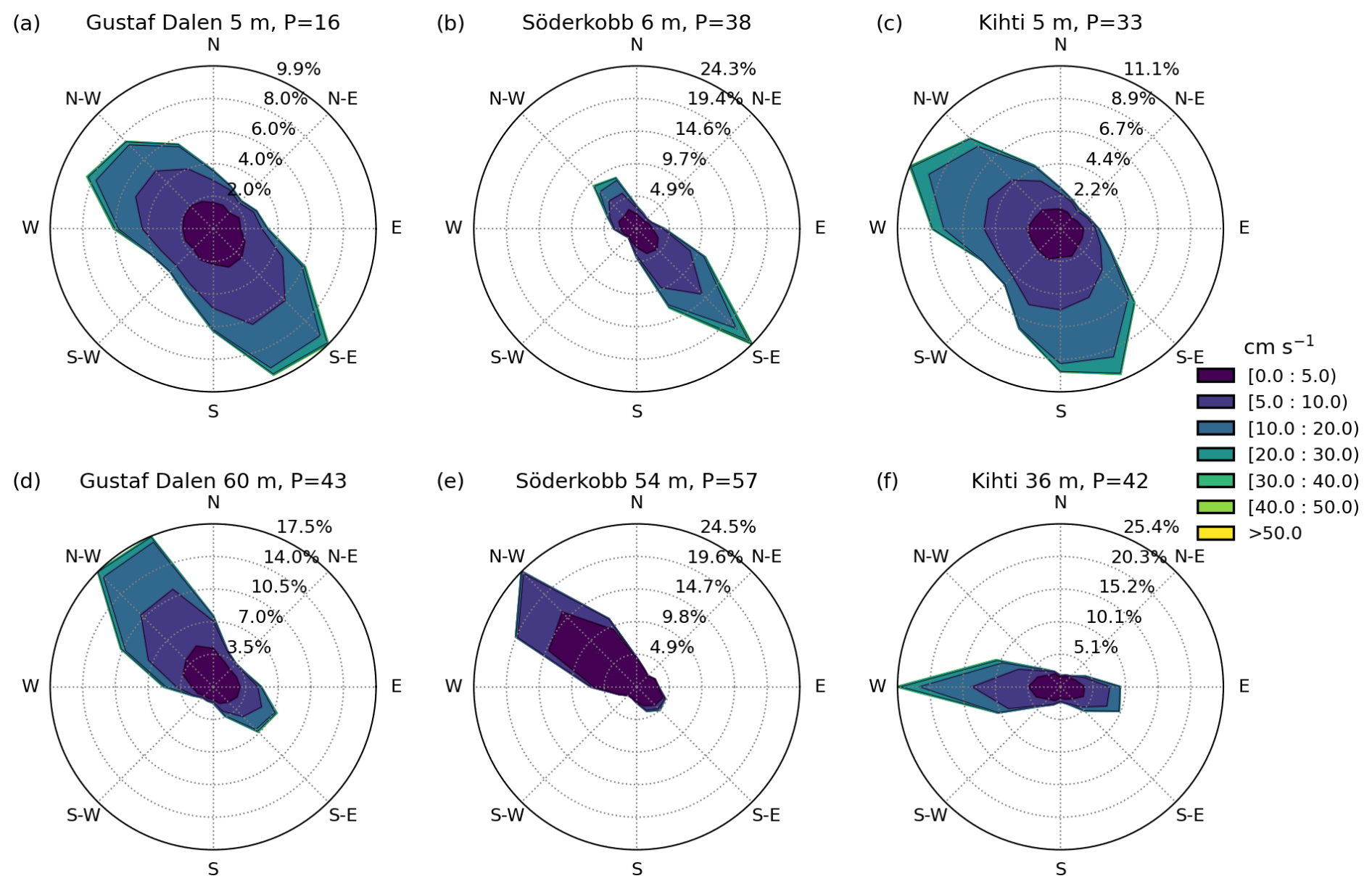
Figure 6 Current roses at the central stations. Panels (a)–(c) show the measurements closest to the surface, and (d)–(f) show the measurements closest to the sea floor (approximately 5 m from the sea floor; Table 2), with the corresponding persistency (P, %). Directions show where the current is flowing to.

At the bottom, the bathymetry (Fig. 1) steers the currents along the deep straits (Fig. 6, lower panels). At the Kihti station, the bottom currents were more frequently towards the west, with occasional flow to the east with a mean magnitude of 7 cm s⁻¹ and P of 42 %. At the Gustaf Dalen and Söderkobb stations, the main direction was towards the NW along the channel at the bottom, with corresponding mean magnitudes of 7 and 3 cm s⁻¹ and P of 43 % and 57 %. The mean magnitude within the entire water column varied between 4 cm s⁻¹ (Söderkobb) and 7 cm s⁻¹ (Kihti and Gustaf Dalen). The maximum magnitudes were measured in the surface layer and ranged from 40 cm s⁻¹ at Söderkobb to 55 cm s⁻¹ at Gustaf Dalen. The low velocities and higher persistency at Söderkobb compared to the other two stations are explained by the seasonality of the measurements (Sect. 3.5).

3.3 Currents in the narrow straits inside the Archipelago Sea

The Norrgrundet, Gloskär, and Lövskär measurements were made in the narrow straits closely surrounded by the islands. Thus, the flow direction was more strongly orientated along the strait throughout the water column. Both of these straits are part of major fairways through the AS where occasional strong currents can affect the navigation of vessels, especially when perpendicular to the ship's course.

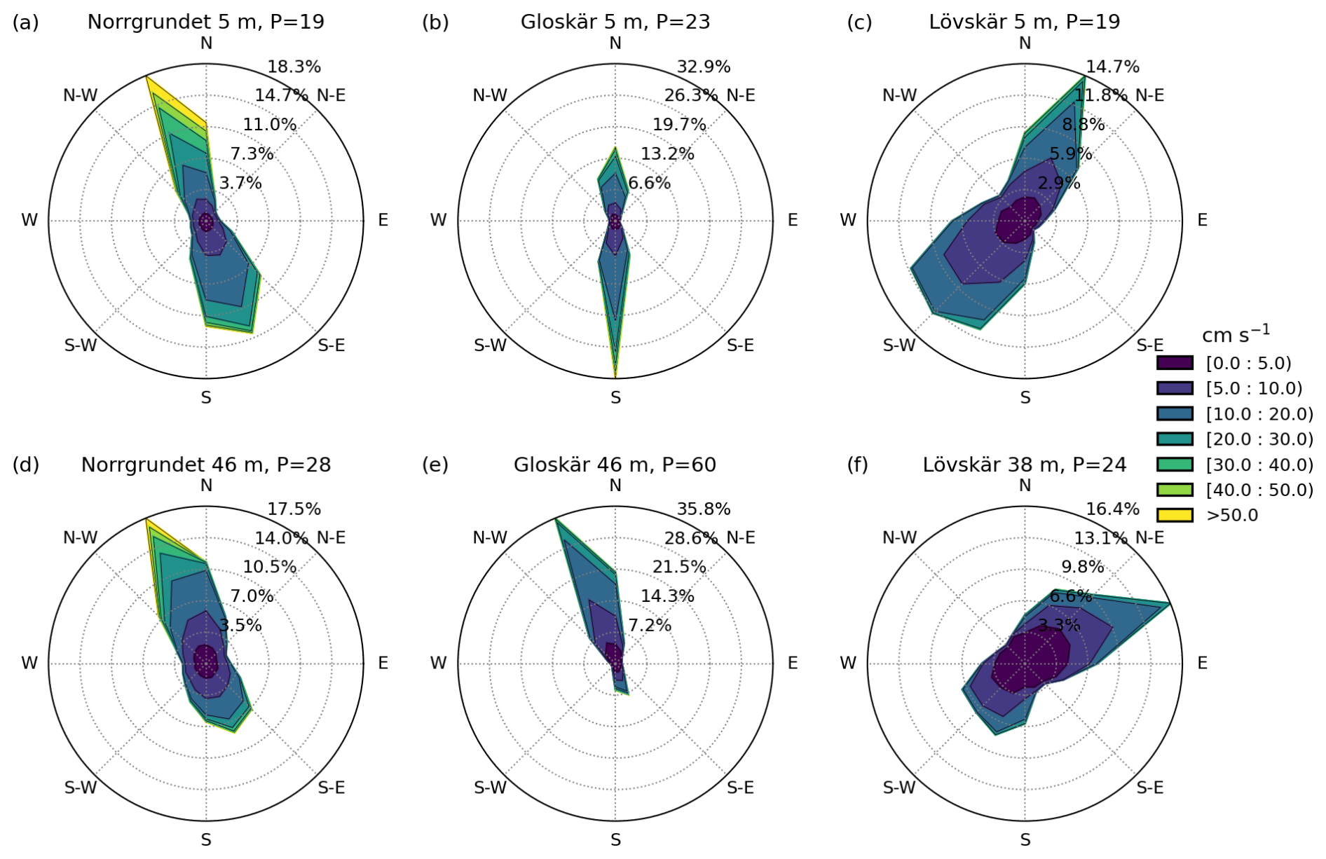
Figure 7 Current roses from the stations surrounded by the dense archipelago. Panels (a) to (c) show the measurements closest to the surface, and panels (d) to (f) show the measurements closest to the sea floor (approximately 5 m from the sea floor; Table 2), with the corresponding persistency (P, %). Directions show where the current is flowing to.

The Norrgrundet and Gloskär stations were located in the same north–south aligned strait, which caused the flow to be strictly aligned towards the NNW or SSE at Norrgrundet with 19 % persistency (P) and toward the N or S at Gloskär with P of 23 % (Fig. 7). At the bottom layer, flow was most frequently towards the NNW at both stations; however, the P at the bottommost measurement depth at Gloskär was around twice (60 %) the one at Norrgrundet (28 %). This is explained by the bathymetry of the area where the Gloskär station was surrounded by a shallower region also at the south (Fig. 8, left panel). These stations have almost double the mean magnitudes compared to other measurement locations in the AS, with the mean magnitude of the entire water column being 14 cm s⁻¹ at Norrgrundet and 11 cm s⁻¹ at Gloskär. The maximum measured magnitudes here reach up to 115 cm s⁻¹ at Norrgrundet and 80 cm s⁻¹ at Gloskär. The flow is slightly stronger in the surface layer, with mean magnitudes of 14 and 17 cm s⁻¹, compared to the bottom layer, with mean magnitudes of 10 and 11 cm s⁻¹, with higher values from Norrgrundet.

The flow speed increases as the water flows into the narrow strait from the more open areas of the north and south. Additionally, wind can further increase the flow speed along the channel. As a result, southward-travelling currents tend to be strongest at the southern edge of the strait and vice versa, as seen from simultaneous measurements of the currents in Norrgrundet and Gloskär (Fig. 8). The distance between the stations is around 28 km (15 nautical miles), and within this distance, the current magnitude increases to around double in the northern end of the channel with northward currents. For southward currents, the increase in magnitude along the channel is slightly less. The Norrgrundet measurements are located at the very end of the strait, thus having a longer overall fetch along the channel than the Gloskär site.

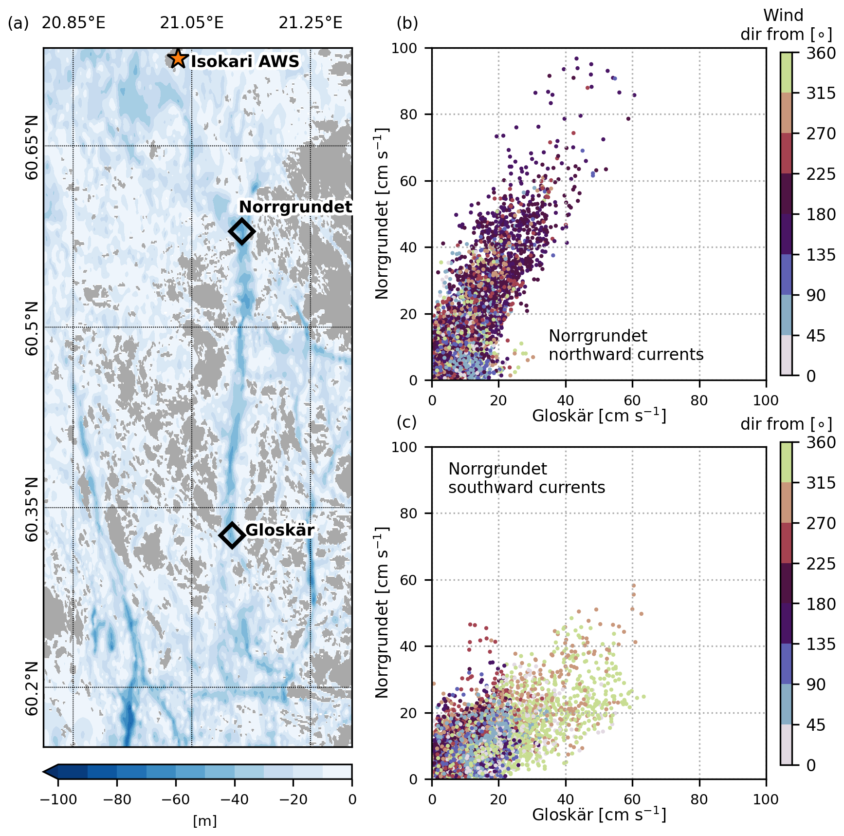
Figure 8 Bathymetry of the narrow northeastern strait (a), and relation between simultaneous measurements (from 20 May to 3 December 2021) of the Norrgrundet and Gloskär current magnitudes at 5 m depth, which is the uppermost measurement layer (b, c). Currents are divided into northward-directed currents (b) and southward currents (c) according to the measured direction at Norrgrundet. The colour bar represents the direction of simultaneous winds measured at the Isokari AWS.

The Lövskär station is located at the end of a much shorter strait than the one where Norrgrundet and Gloskär are located. The Lövskär measurements were carried out in the cross section of two shallow straits and thus also in the most open area at that location (Fig. 1). Flow at Lövskär was mainly toward the SW or NE; however, bathymetry and geometry steered currents at the surface more toward the NNE, with a mean magnitude of 9 cm s⁻¹ and P of 19 %, and at the bottom towards the NEE, with a mean magnitude of 6 cm s⁻¹ and P of 24 % (Fig. 7, rightmost panels). NE currents have been shown to be mostly caused by southeasterly winds, whereas SW currents were driven by northerly winds (Kanarik et al., 2018). The maximum measured magnitude at this station was 49 cm s⁻¹, with the mean magnitude throughout the water column being 7 cm s⁻¹.

3.4 Currents at the northern edge of the Archipelago Sea (in the southern Bothnian Sea)

The northernmost measurements (Norrskäret and Norra Bredan) were located at the northern ends of the westernmost and central straits coming out of the AS (Fig. 1). The mean magnitude of the currents measured throughout the water column in Norrskäret was 4 and 10 cm s⁻¹ in Norra Bredan. The large difference between these areas is partly explained by the seasonality of these measurements, which is discussed in more detail later in Sect. 3.5.

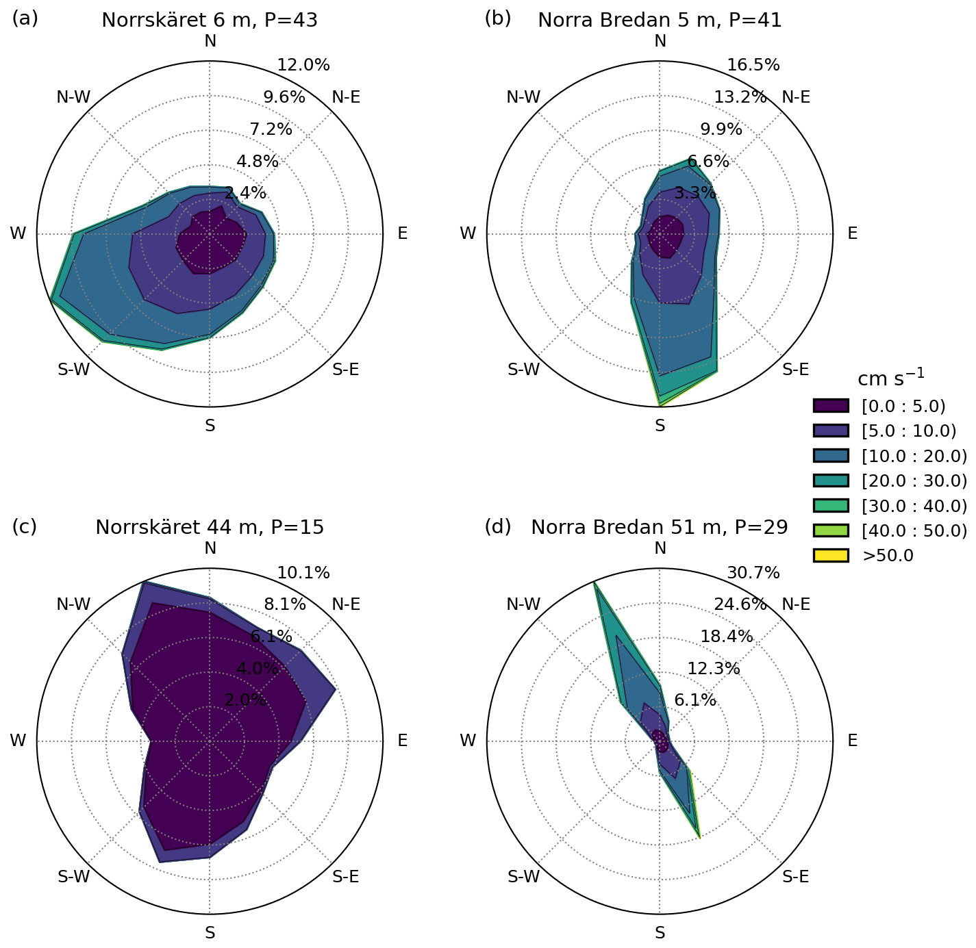
Figure 9 Current roses from the northern stations. Panels (a) and (b) show the measurements closest to the surface, and panels (c) and (d) show the measurements closest to the sea floor (approximately 5 m from the sea floor; Table 2), with the corresponding persistency (P, %).

The currents in Norrskäret were most frequently toward the WSW at the surface (Fig. 9, Norrskäret), with a mean magnitude of 8 cm s⁻¹ and P of 40 %, while there was no clear main direction of the flow at lower depths, with a mean magnitude of 3 cm s⁻¹ and P of 15 %. Overall, flow at the bottom in Norrskäret was more towards northward directions than southward. The directionality was quite different at the northeastern station – Norra Bredan. There, the flow was most frequently towards the south at the surface, with a mean magnitude of 9 cm s⁻¹ and P of 41 %. Norra Bredan was located in the centre of a narrow strait that strongly steered currents at the bottom layer, and thus the flow was mainly along the canyon (NNW/SSE) with P of 29 %. The currents in the bottom layer at Norra Bredan were often stronger than at the surface, with the mean magnitude in the bottom layer being 12 cm s⁻¹. The strongest currents in this bottom layer reached 62 cm s⁻¹ and were toward the SSE. The highest value measured in the surface layer of these areas was 50 cm s⁻¹ at Norrskäret and 52 cm s⁻¹ at Norra Bredan.

3.5 Seasonal statistics of the current magnitudes

The current speeds varied greatly between different measurement locations around the AS. The strongest currents were measured in the long narrow strait in the northeastern AS (Norrgrundet and Gloskär) and at the end of another long strait by the northern edge of the AS (Norra Bredan). The weakest currents were measured in more central regions of the AS. Currents can have large seasonal and year-to-year variations due to variability in the meteorological and sea ice conditions and due to stratification. Thus, the magnitudes of the currents at each station with different measurement periods are not directly comparable (Table 1, Fig. 2). To get an overview of the spatial and temporal differences, seasonal statistics for each station were calculated over the whole water column (Fig. 10) using hourly averaged current magnitudes to account for different measurement frequencies (Table 2). Note also that not all stations have measurements that cover all seasons. For example, very few measurements are available for Lövskär during spring (Fig. 10b), Norra Bredan during summer (Fig. 10c), and Fölskär during autumn (Fig. 10d). Moreover, several stations do not have measurements for all four seasons, which limits the temporal comparability of the results (Fig. 10).

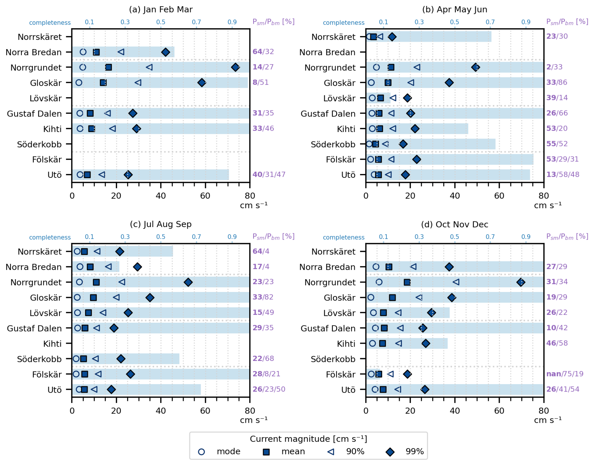
Figure 10 Seasonal statistics calculated from hourly mean current magnitudes over all depth bins. The values 90 % and 99 % represent the 90th and 99th percentiles of the current magnitudes. Persistency values are given seasonally to each station's surface-most (P_bm, bolded values) and bottommost (P_bm) depth cells (corresponding depths can be found in Figs. 5, 6, 7, and 9). An additional persistency value is given for the stations at the southern edge of the AS (Fölskär and Utö), with the occasional halocline given between the P_sm and P_bm values. The completeness of the dataset of each season is given relative to the top x axis as blue bars, where a value of 1 stands for at least one complete season of measurements with no large data gaps, e.g. 0.5 indicates that during this season, the measurements cover only around 1.5 months out of the 3 per season.

The seasonal means of the current magnitudes (Fig. 10) are quite uniform within each season throughout the AS. In most of the AS stations, the measured currents were weakest during spring when mean magnitudes varied between 5 and 6 cm s⁻¹. The currents were strongest in winter and autumn with mean magnitudes between 7 and 9 cm s⁻¹ in winter and 6 and 8 cm s⁻¹ in autumn. The mean magnitudes in summer ranged between 5 and 7 cm s⁻¹. Note that the most frequently measured values (mode) are below the mean value. The variations between different stations were larger when looking at the distribution of the highest 99th percentile of the current magnitudes. Extreme cases were typically caused by single storms, and the occurrence of these cases can vary largely in our heterogeneous dataset. We present the 90th percentile of the current magnitudes together with the 99th percentile first to represent the rarity of the extremes and second to give an overview of the data distribution together with the mode (Fig. 10).

The largest variation in the current magnitudes between the measurement stations occurred during the winter season, when winds are typically strong (Fig. 4) but occasionally the ice cover hinders the local winds from inducing currents. Winter also has the fewest measurements of all four seasons. Winter poses challenges to the ADCP measurements, and typically some data had to also be discarded due to bad data quality for the Norrgrundet, Gustaf Dalen, and Utö stations (Check Sect. “Quality issues” under Sect. 2.1). Statistics are calculated only from good-quality data, and thus current magnitudes in the winter represent mainly conditions during ice-free periods.

The mean and 99th percentile magnitudes of the Norrgrundet and Gloskär currents are almost twice the values measured in other areas of the AS (Sect. 3.3 and Fig. 10), most notably in winter (panel a) and spring (panel b) months. The strongest currents in the area were measured at the Norrgrundet station. The mean magnitudes for all seasons varied between 11 and 19 cm s⁻¹, with the weakest magnitudes measured in summer and the strongest in autumn. One-tenth of the measurements (90th percentile) exceeded the magnitudes of 23–41 cm s⁻¹, and 1 % of the measurements (99th percentile) exceeded values from 50 to 74 cm s⁻¹. The currents measured at Gloskär, in the slightly more central area of this strait, were slightly weaker and had a different distribution compared to those in Norrgrundet. The most frequent current magnitude (mode) was weaker than or on the same order of magnitude as at other stations in the AS. However, the mean, 90 %, and 99 % values were clearly higher (or on the same order of magnitude as at Norra Bredan in the northern edge of the AS) than at the other stations outside of this strait. This means that strong currents occur more frequently in this strait than at the other measurement stations, although most of the currents at this station are on the same order of magnitude as at other locations in the AS, with a mode of around 3 cm s⁻¹. The mean magnitudes ranged from 10 cm s⁻¹ to 14 cm s⁻¹, 10 % of the values exceeded 20–30 cm s⁻¹, and 1 % exceeded 37–58 cm s⁻¹, with the weakest statistics always measured in spring and summer and the strongest in winter.

During time periods when a seasonal thermocline was present, the measured currents at both Norrgrundet and Gloskär were significantly weaker in the bottom layer than at the surface (Fig. 11): the mean magnitude in the bottommost layer was around 6 cm s⁻¹ at Norrgrundet and 8 cm s⁻¹ at Gloskär.² The flow direction of the lower layer during stratification was mainly towards the north (Fig. 11b and d), as also seen in Miettunen et al. (2024). The persistency was only slightly stronger at Norrgrundet during time periods when a seasonal thermocline was present (P of 32 %) than the overall P in the bottom layer (28 %), but at Gloskär, P increased to 84 % due to the stratification compared to the overall 60 %. These low current magnitudes below the thermocline during the summer season caused the mean current speeds (Fig. 10) to be more similar to the mean values of the other AS measurement stations outside of the strait. However, when we compared only surface layer statistics at Norrgrundet and Gloskär (not shown), current magnitudes in the summer followed the same trend as in other seasons, being almost twice the magnitude measured in other regions. Although currents below the thermocline were noticeably weaker than at the surface, there were events where the current magnitude in the bottom layer reached magnitudes up to 30 cm s⁻¹ at Norrgrundet and 38 cm s⁻¹ at Gloskär, with the 99th percentile of values reaching 20 cm s⁻¹ at Norrgrundet and 26 cm s⁻¹ at Gloskär.

As at Norrgrundet and Gloskär, most stations showed slightly higher persistency values near the bottom compared to the surface layer (Fig. 10). When examining seasonal persistency, the measurements show substantial variation not only between different seasons but also between nearby stations that were measured during different years.

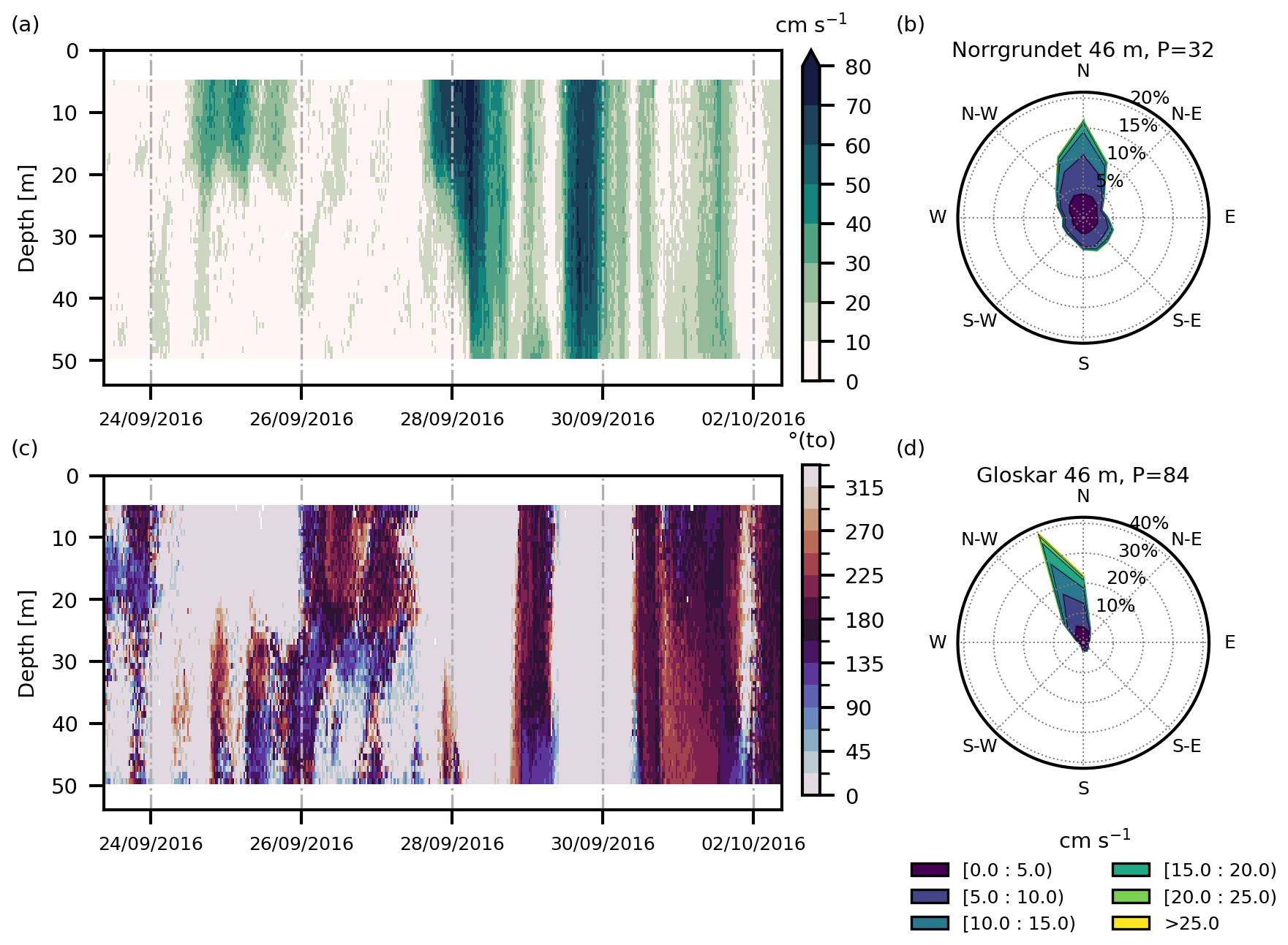
Figure 11 Depth profiles of current magnitudes (a) and directions (c) at the Norrgrundet station before and after seasonal overturning on 28 September 2016. The thermocline can be seen at a depth of 20–30 m. Current roses for Norrgrundet (b) and Gloskär (d) at approximately 46 m depth during the stratified measurement periods with the corresponding persistency (P, %). The Norrgrundet data cover the time periods from 6 to 28 September 2016, 5 June to 5 September 2017, and 17 June to 18 August 2021. The Gloskär data cover the time periods from 17 June to 20 September 2021 and 22 April to 2 June 2022.

4 Drivers of strong currents

The Archipelago Sea serves as a route for maritime transport and is crossed by several fairways. Providing information on strong currents is important for maritime safety in this area, and therefore understanding the drivers of these currents is necessary. We will focus our analysis on the long and narrow strait in the northeastern AS (Sect. 3.3 and Fig. 8). The Norrgrundet station at the northern end of the channel had the highest current magnitudes of the entire measurement dataset (Sect. 3.5).

There were altogether 224 events during approximately 30 months of measurement time series, where the current speed exceeded 40 cm s⁻¹. The median and maximum duration of these events were 5.5 and 35 h, respectively, which constituted almost 8 % of the measurements. Most of these strong current events (ca. 75 %) aligned with the wind direction, while about one-quarter opposed the wind direction for the majority of each event's duration. These events were defined by studying the simultaneous winds during high current events and classifying the events based on the prevailing wind direction. As this dataset included numerous high current events, we chose to present a few time-specific events that demonstrate the main features of the different cases identified.

Strong current events are often the result of the combined effect of wind and differences in sea level. These forcings can work in the same direction, supporting each other, or in different directions, opposing each other. The complicated geometry of the AS region causes the growth of currents driven by local winds to be highly sensitive to the wind direction. Even a slight shift in the wind direction can cease the growth of the currents. This pronounced sensitivity to wind direction for AS currents has previously been demonstrated in the narrow Lövskär cross section (Kanarik et al., 2018). In the north–south aligned strait studied here, the strongest currents typically occur with strong northward (Fig. 12a) or southward (Fig. 12b) winds, provided that the opposing sea level difference across the AS is not significant. When winds are weak or misaligned with the strait's geometry, the sea level difference across the AS can become the dominant driver of strong currents (indicated by the ellipse in Fig. 12a). Typically, the largest sea level differences across the AS coincide with strong opposing winds, meaning that the strongest currents rarely align with the highest sea level differences.

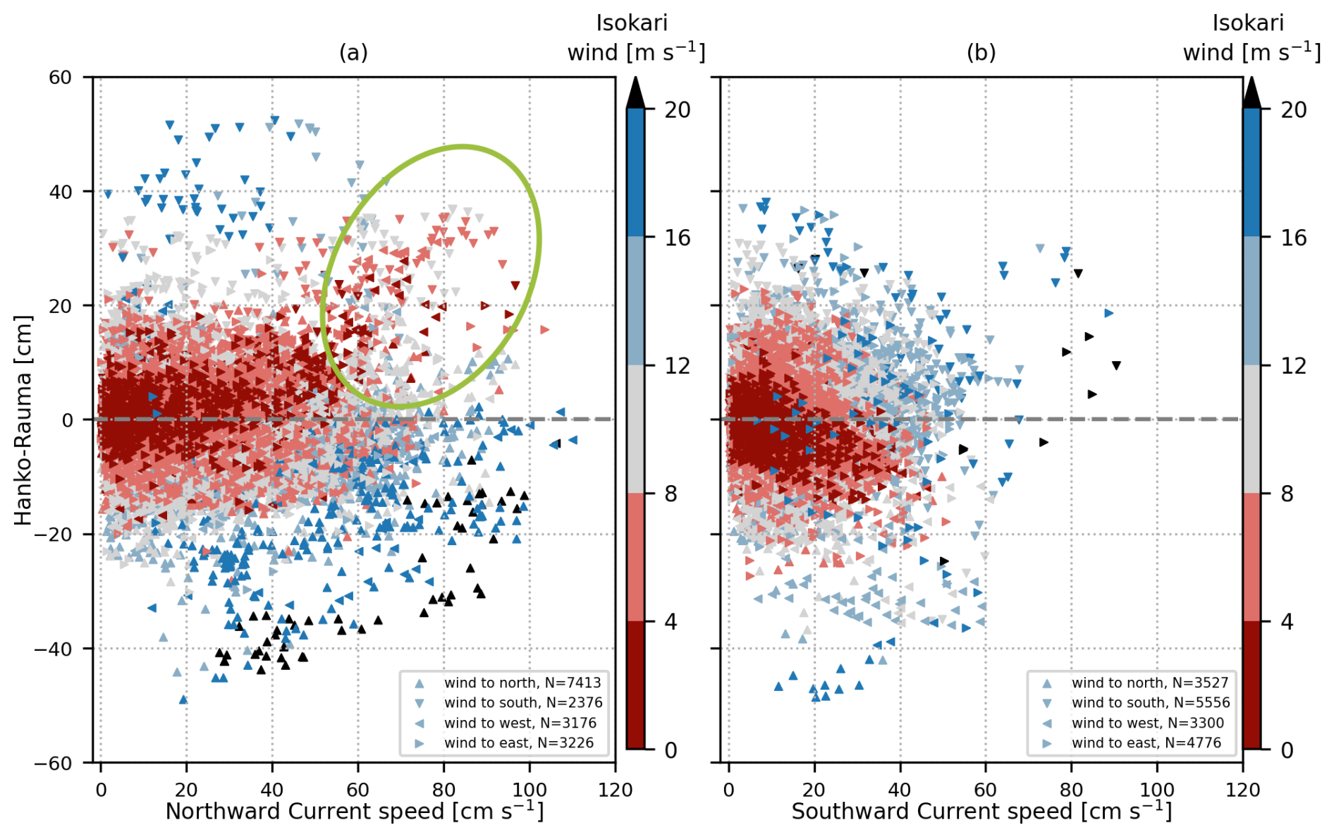
Figure 12 Norrgrundet current magnitudes against the sea surface height difference between Hanko and Rauma. The data are divided into two main current directions: northward currents (a) and southward currents (b). The corresponding wind speed is presented as a colour, and the main wind direction is indicated by a marker arrow. Positive sea level difference drives currents northward and vice versa. Northward wind direction is defined as >315° and ≤45°, and the other three main compass directions are defined correspondingly. N indicates the number of different data points in each scatter. The scatter data are sorted so that the points with the smallest wind speeds are overlaid on top, up to a magnitude of 16 m s⁻¹. Rare, over 16 m s⁻¹ winds and higher are at the very top of the scatterplot. Northward currents driven by a large sea level difference caused by the oscillation in the surrounding basins are highlighted with an ellipse in (a).

During the strongest current event, with a magnitude of 115 cm s⁻¹, on 22 February 2017 (Fig. 13), both the wind and the sea gradient drove the northward flow, which was further amplified by changes in atmospheric pressure fields over the Bothnian Sea. In addition to wind and sea level pressure forcing, the narrowness of the channel further amplified the flow (Fig. 8). SSE winds of around 20 m s⁻¹ blew for several hours, and during this time, the sea level at Föglö was about 9 cm higher than at Rauma and Hanko (see the locations of the tide gauges in Fig. 1). The current speed grew until the winds turned to a less optimal direction relative to the strait (Fig. 13). The growth of high current events was most often stopped by the turning of the wind; thus, the maximum values presented in Fig. 12 often measured simultaneous winds from either the east or west.

The second-strongest event, with a magnitude of 104 cm s⁻¹, on 28 December 2016 (Fig. 14) was driven by a sea level difference across the AS, with the wind blowing in the opposite direction. During this event, a sea level difference of several tens of centimetres (up to 31 cm) between Hanko and Rauma counteracted the northerly winds, and this produced strong northward currents that flowed against the wind once the wind speed had decreased below 10 m s⁻¹. Note that the highest spike in current magnitude occurred when local winds shifted to blowing along the strait. During this event, sea levels in the Gulf of Finland (Hamina measurements) had started to oscillate after the winds had piled up water at the head of the Gulf of Finland on 24 December 2016, initiating a seiche. By 28 December, the sea level in the Gulf of Bothnia dropped (Kemi measurements), and the resulting seiche oscillation in the Gulf of Finland created a strong sea level gradient across the AS, one that was able to drive currents against the now-weakened local wind. A similar event was observed between 24 and 26 February 2017, following the strongest measured currents (Fig. 13). These types of events in general are also well visible in comparison with current speeds, sea level differences, and wind magnitudes in Fig. 12, highlighted with an ellipse. There are numerous events where sea level gradients drive strong northward currents. The phenomenon is not as visible in southward currents, as the geometry of the strait further enhances the current speed, but it is still present. Events related to the seiche in the Gulf of Finland appear more clearly in comparison to the Hanko and Rauma tide gauges than between Föglö and Rauma, which, in general, better represents the sea level gradient over the AS. During events with strong seiche, the sea level is also simultaneously higher in the SE corner (Hanko) of the AS than in the SW corner (Föglö).

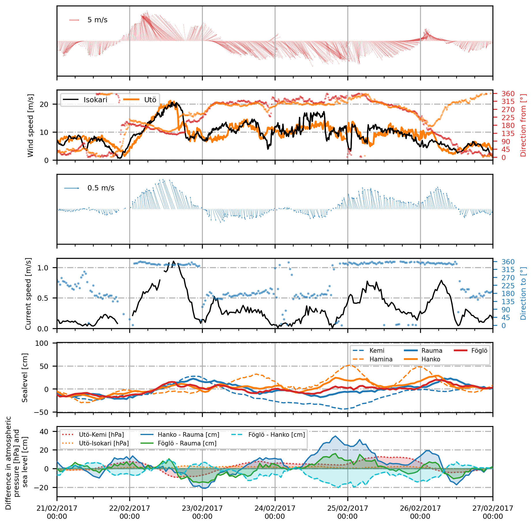
Figure 13 Time series of the strongest current event in Norrgrundet (22 February 2017) followed by seiche-induced wind-opposing currents. The time series shows simultaneous winds, currents, and sea levels together with the differences in sea level and atmospheric pressure in northern (Isokari and Rauma) and southern (Utö, Hanko, and Föglö) edges of the Archipelago Sea (see the map in Fig. 1). Föglö represents sea levels in the southwestern AS, and Hanko, in the southeastern AS. Measurements at Kemi represent the conditions at the northern end of the Gulf of Bothnia, and measurements at Hamina represent the eastern Gulf of Finland. The first and second panels present wind speed and direction at Isokari, and the third and fourth panels present currents at the uppermost layer measured at Norrgrundet (5 m depth). The upward arrow indicates the northward direction for both wind and current measurements. The fifth panel presents the sea level variation around the AS (solid lines) and at the end of the surrounding basins (dashed lines). The lowest panel shows the differences in sea level and atmospheric pressure between various stations around the AS.

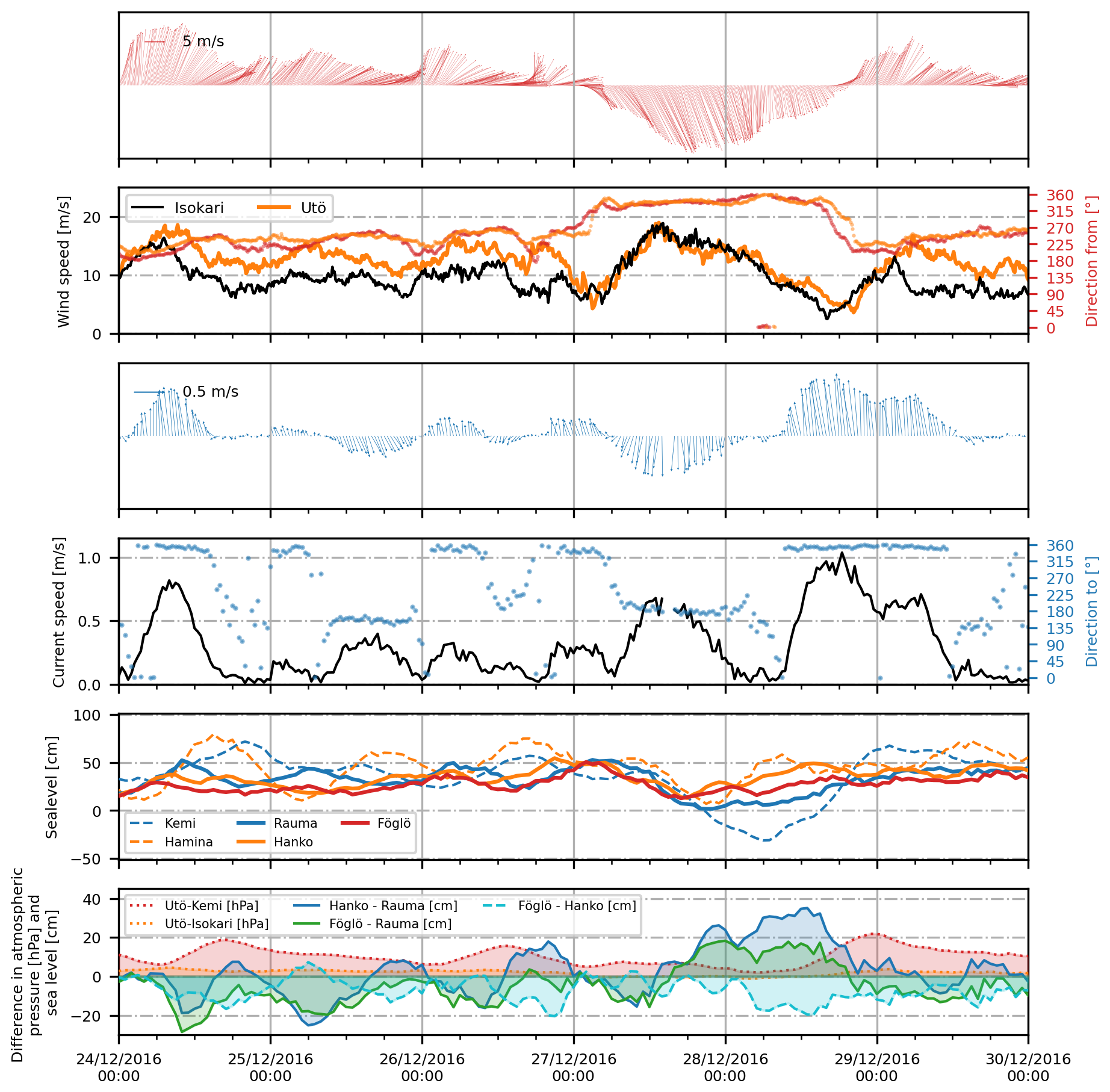
Figure 14 Time series of the second strongest current event in Norrgrundet (28 December 2016) with simultaneous wind and sea level measurements together with sea level and atmospheric pressure differences from the surrounding stations (Fig. 1). The first and second panels present the wind speed and direction at Isokari (and Utö, included in orange in the second panel), and the third and fourth panels present currents at the uppermost layer measured at Norrgrundet. The upward arrow indicates the northward direction for both wind and current measurements. The fifth panel presents the sea level variation around the AS (solid lines) and at the end of the surrounding basins (dashed lines). The lowest panel shows the differences in sea level and atmospheric pressure between various stations around the AS.

Mostly, the effect of opposing the sea level gradient relative to the wind direction only weakens the effect of local winds, whereas currents still follow the direction of the winds. During the storm Toini on 11 January 2017 (Fig. A2), the winds at Isokari were up to 22.5 m s⁻¹ and stayed around 20 m s⁻¹ for more than 18 h. The maximum current was 99 cm s⁻¹, being the third-strongest event and having the longest-lasting duration of currents over 40 cm s⁻¹ (35 h). These were the strongest winds measured during the 30 months of measurement at the Norrgrundet station, and the storm resulted in record significant wave height measurements by the Northern Baltic proper wave buoy (Björkqvist et al., 2017). However, during the event, the sea level difference quickly rose to oppose the currents, being around 20 cm higher at Rauma than at the Föglö and Hanko stations in the south, and finally the seiche in the Gulf of Finland made the sea level difference increase to 44 cm higher at Hanko than at Rauma. At the highest sea level difference, the current speeds had already decreased significantly. However, the currents did not begin to follow the sea level gradients until the wind speeds dropped below 10 m s⁻¹.

During non-optimal wind conditions, the sea level difference was the dominant factor driving the currents (as seen between 26 and 31 August 2021 in Fig. A1 in Appendix A). Although easterly winds do not directly induce currents in the measured channel, they do affect the sea level in more open sea areas, like at the northern edge of the AS, thus contributing to the lower sea levels measured at the Rauma station in this case.

It is notable that in the AS, when the wind and the sea level gradient support the same flow direction, the wind speed does not need to be very high to induce strong currents (grey and light blue colours in the lower-right corner of the ellipse in Fig. 12). For example, on 18 August 2021 (Fig. A1), the SSE wind only briefly reached the maximum of 16 m s⁻¹ and stayed mainly only slightly above 10 m s⁻¹, while simultaneously the water was high at the SE corner (represented by the Hanko measurements) of the AS, with the sea level around 10 cm higher at Hanko than at Föglö and Rauma. Together, these resulted in up to 97 cm s⁻¹ current speeds at the Norrgrundet station, which is the fourth-highest magnitude measured at this station.

4.1 Statistics of drivers

There are decades of atmospheric and sea level measurements from automatic weather stations (AWSs) and tide gauges along the Finnish coast (Sect. 2.2). As our current measurements consist only of short datasets (Table 1), we extended our analysis to the statistics of the drivers identified as significant around the AS. We used a 30-year reference period from 1991 to 2020 to see the frequency of occurrence of high sea level differences and wind speeds. Continuous atmospheric pressure data were available only from 2007 onwards (Sect. 2.2).

4.1.1 Local winds

On average, the Utö AWS in the south measures slightly higher winds compared to the Isokari AWS in the north. Three-hourly measurements from 1991 to 2020 show that the mean wind speed was 7.5 m s⁻¹ at Utö and 6.9 m s⁻¹ at Isokari, with the 99th percentile of the wind speeds being 18 and 16 m s⁻¹, respectively. The maximum measured wind speed during the 30-year reference period was 29 m s⁻¹ at Utö and 27 m s⁻¹ at Isokari, both measured on 14 October 2010. The seasonality of the local winds is briefly described in Sect. 3 and presented in Fig. 4, showing that the winds in the region are stronger in autumn (OND) and winter (JFM) than in spring (AMJ) and summer (JAS). For example, at Isokari, 99 % of the winds exceeded 14 m s⁻¹ during the spring and summer months (AMJ and JAS), while the same percentage exceeded 18 m s⁻¹ in autumn (OND) and 17 m s⁻¹ in winter (JFM). Although record-high winds were measured in autumn, up to 22 m s⁻¹ winds were measured in spring and 25 m s⁻¹ in summer at the Isokari station.

During our 30-month measurement period at the Norrgrundet station, the distribution of the wind speeds followed rather closely the one from the climatological reference period, with 99 % of winds exceeding 17 m s⁻¹ at both Utö and Isokari. However, the maximum measured wind speed of 23 m s⁻¹ (storm Toini, Fig. A2) was still far from the maxima measured during the reference period.

4.1.2 Sea level differences

The 30-year reference period for tide gauge measurements compared to theoretical mean water shows that, on average, the water level is slightly higher at Rauma than at Hanko, with a mean difference of 0.9 cm. However, extreme differences where the water level is higher at Hanko than at Rauma are slightly more frequent, with 1 % of values being greater than 22 cm and 0.1 % being greater than 39 cm, than those where the water is higher at Rauma than at Hanko, with 1 % of values being greater than 19 cm and 0.1 % being above 31 cm. Similar values are seen when looking at the sea level differences from a slightly different angle of the AS, as, on average, the sea level is 1.4 cm higher at Rauma than at Föglö, with 98 % of the difference varying between −17 to 14 cm (Föglö–Rauma).

Compared to the 30-year reference period, the Norrgrundet measurement time series reflected the typical distribution of sea level differences. The event on 28 December 2016, which featured maximum current speeds under opposing winds (Fig. 14), was notably rare, with a sea level difference of 31 cm corresponding close to a 0.1 % occurrence frequency. Comparisons indicate that sea level differences across the AS can exceed those observed in our relatively short 30-month dataset by several tens of centimetres. During the 30-year reference period, the maximum measured sea level difference was 71 cm between Hanko and Rauma and 59 cm between Föglö and Rauma.

4.1.3 Atmospheric pressure difference

To account for the inverse barometer effect, we examined measurements of atmospheric pressures over the AS, as strong atmospheric pressure differences can weaken or enhance the currents driven by the sea level difference. Sea level gradients caused by atmospheric pressure differences over the AS (measured between the Utö AWS and Isokari AWS) typically vary by only a few cm (or hPa) across the approximately 100 km distance between the two weather stations.

Simultaneous measurements, from 2007 to 2020, show that atmospheric pressure differences (Utö–Isokari) range between −3 and 4 hPa for 98 % of the time. The maximum observed differences during the measurement period ranged from −6 to 10 hPa. In the time series (Figs. 13 and 14), we also present the atmospheric pressure difference between Utö and Kemi, which are about 7 times farther from each other than are Utö and Isokari. Between Utö and Kemi, the pressure difference varied 98 % of the time between −13 and 20 hPa, with the maximum measured differences being −28 and 29 hPa.

As the 1 hPa difference is equal to a 1 cm difference in sea level over the same distance, we see that the maximum tilt to the sea surface caused by the atmospheric difference over the AS has been at most 10 cm, and in 98 % of the cases, it was less than half of this.

During the 30-month measurement period at Norrgrundet, the maximum difference in atmospheric pressure between Isokari and Utö was 5 hPa in both directions. When looking at the strongest measured current events (Figs. 13 and 14), the atmospheric pressure difference has been at most 20 hPa over the entire Gulf of Bothnia (Utö–Kemi) and around 3 hPa over the AS (Utö–Isokari).

5 Discussion

As this analysis is performed by combining measurements from numerous short campaigns, the measurement setups are not consistent with each other. Different measurements had varying depth cell size ensemble intervals and numbers of pings per ensemble, causing the standard deviation to vary between 0.7 and 1.75 cm s⁻¹ (Table 2). Our measurements had multiple cases where measurements were not successful due to non-optimal conditions at sea. The main scatterers in the right size range for 300 kHz ADCPs are zooplankton, which can be clearly seen from the analysis of the echo intensity of the signals at each site (Karvo, 2023). The signal quality appeared to be especially poor in spring seasons after winters with substantial ice cover in the AS. However, this paper does not focus on the reasons behind these data gaps, as they most likely have a strong biological background. Data were simply flagged as good on the basis of quality parameters provided by the instrument. As the prevailing weather conditions have large seasonal as well as year-to-year variations, a direct detailed comparison between all the measurement sites should be made with caution. The maximum current speeds presented reflect only peaks during the measurement campaigns, and these depend on the type of storms in the area at that time. However, compared to previous measurements in the area (Virtaustutkimuksen neuvottelukunta, 1979; Ambjörn and Gidhagen, 1979; Kanarik et al., 2018), the measurement campaigns presented in this study had a larger coverage in both time and vertical extent (covering almost the entire water column), allowing us to catch extreme current speeds caused by sea level fluctuations in the basins surrounding the AS.

We made seasonal analysis of the current magnitudes to make the measurements from different years and seasons more comparable. This analysis showed that narrow long straits significantly enhanced current speeds, being approximately twice the magnitude of the other areas, which mostly showed similar statistics to each other (e.g. mean speed around 8 cm s⁻¹). Our measurements, for the first time, show measured currents of 1 m s⁻¹ in the AS. Although our measurements were performed only in one of the long north–south aligned straits of the AS, recent model analysis on circulation in the area (Miettunen et al., 2024) shows that the other straits show similar behaviour. In addition, one of the earlier measurement campaigns by Ambjörn and Gidhagen (1979) measured 91 cm s⁻¹ currents at the southern end of one of the other northern straits (north of Gustaf Dalen, as shown in Fig. 1).

An early study on general circulation of the Baltic Sea that was based on current observations from lightships (Witting, 1912) indicated that there are seasonal differences in the persistency of surface layer currents in the coastal regions of the Bothnian Sea and in the Gulf of Finland. That study also concluded that there is outflow from the Bothnian Sea through the Archipelago Sea in early summer and inflow to the Bothnian Sea through the Archipelago Sea in autumn. We calculated the seasonal persistency of currents in the Archipelago Sea (results shown in Fig. 10). Our results do not confirm such a clear resultant circulation pattern to be present in the AS. Especially in autumn, the persistence of the currents seems to be smaller. This is in accordance with the rather low persistency of winds in monthly statistics of 2000–2016.

In general, our measurements show a very similar directional distribution of the currents as presented in the model simulations by Miettunen et al. (2024), although the measurements and model results cover different time periods. The focus of these model studies is the overall circulation and transport dynamics of this area and thus are not as comparable to our findings based on measured data. In the future, combining information with measurements with suitable circulation modelling will lead to a more comprehensive overview of the circulation dynamics also in those areas from which we lack measurements. Our findings encourage taking a closer look at single storms and large oscillation events in the surrounding basins (like in Fig. 13) to quantify their significance to the water exchange through the AS.

Our analysis was supported by weather station and tide gauge measurements from the AS and its neighbouring basins, i.e. the Gulf of Bothnia, Baltic proper, and the Gulf of Finland (Fig. 1). These measurements represent the conditions in the surrounding basins and provide an overview of larger-scale phenomena that affect the dynamics of the AS. However, because weather and sea level measurements are from different areas around the AS (Fig. 1), analysing the simultaneous effects of these drivers on currents, again at different locations, is challenging and prohibits a comprehensive overview of the different effects and their combinations.

The complicated configuration of islands and narrow channels of the AS affects the wind fields as well. The islands also have different topographies, and some are covered with dense forests. These can cause channelling effects on the wind field in narrow straits, strengthening the winds (e.g. Chaudhari et al., 2023). This can then further enhance the current speeds. As there are no wind measurements available near the narrow straits, we could not quantify the effect. Considering a textbook example of surface currents being around 2 %–3 % of wind speeds in the open sea, extreme wind events, with 30 m s⁻¹ speeds, could induce a current speed of up to 60 to 90 cm s⁻¹ in idealised open sea conditions. The 2 %–3 % estimate from the strongest measured winds of 23 m s⁻¹ (storm Toini) during our measurement time series would give an estimate of 50 to 70 cm s⁻¹ currents. The measured maximum of the currents at Norrgrundet during the storm Toini was 99 cm s⁻¹, so the channelling effect makes a significant contribution to the current speed in this narrow strait (Fig. 8). When considering the overall magnitudes of the surface current in the AS, where the mean magnitudes vary from 8 cm s⁻¹ in more open areas to around 14 cm s⁻¹ in narrow straits, the 2 %–3 % estimate of mean wind speeds would largely overestimate the currents by giving a magnitude range from 14 to 22 cm s⁻¹.

Although atmospheric pressure fields and sea level differences work hand in hand in driving the sea currents, they could not be used directly together in these analyses. However, we can still get an overview of the sea level gradients. Section 4.1 describes the long-term differences in sea level and atmospheric pressure over the AS and shows that although the atmospheric pressure differences can be quite large, the differences are clearly smaller than the largest differences observed in sea level (Sect. 4.1.2 and Fig. 12). Looking at the highest and lowest 1 % of the differences over the AS, the atmospheric pressure difference between Utö and Isokari is approximately a quarter of the difference between Hanko and Rauma. To have a more exact comparison, sea level fields could be interpolated to the Utö and Isokari AWS locations using the surrounding three tide gauges. If we were to consider an idealised situation using these highest and lowest 1 % of the sea level differences between Hanko and Rauma (around 20 cm) over a distance of around 200 km between the two stations, this tilt could drive geostrophic currents of around 8 cm s⁻¹. The highest and lowest percentage of atmospheric pressure difference between Utö and Isokari (around 100 km apart) varied between 3 and 4 hPa. Considering again an idealised situation where the 3 hPa air pressure difference would quickly change to equilibrium, this difference could drive currents of around 1 cm s⁻¹. If we were to consider the rather unlikely condition of atmospheric pressure changing from one 1 % extreme to another and thus changing the equilibrium by 7 hPa, this could drive currents up to 3 cm s⁻¹. Currents possibly driven by atmospheric pressure changes are thus clearly weaker than the ones driven by overall sea level differences.

Comparison to idealised current speeds over the area also shows that none of these forcings is strong enough to induce currents as large as the wind can. The maximum sea level difference during our Norrgrundet measurements was 31 cm between Hanko and Rauma, and under ideal conditions, this could induce geostrophic currents of up to 12 cm s⁻¹, while 23 m s⁻¹ winds could be estimated to generate currents well above 50 cm s⁻¹. Of course, these analyses are theoretical and thus are not suitable for the complex conditions of the AS.

When considering safe navigation in the Archipelago Sea, these measurements show that high currents typically occur with high and storm wind events. However, considering also the events where high current speeds occur during relatively calm weather induced by sea level differences, it is difficult to make any simplified cause-and-effect relationship solely based on wind forcing, as also shown in Fig. 12. To issue warnings of high current events, a high-resolution operational model would be needed.

6 Conclusions

We analysed and presented current measurement datasets from the Archipelago Sea (AS). We described the general features of the measured currents and examined the drivers of the strong currents in the area.

Measurements in the AS can be divided into two types based on current magnitudes: more open sea areas with a mean surface layer current magnitude of around 8 cm s⁻¹ and narrow long straits with a mean surface current magnitude of around 14 cm s⁻¹. All of our datasets have measured currents of at least 40 cm s⁻¹. In more open areas, maximum currents typically varied between 50 and 60 cm s⁻¹, but currents up to 115 cm s⁻¹ have been measured in narrow straits. However, these high values are still rare, as 90 % of the measurement values were below 10 to 20 cm s⁻¹ and 99 % of the values were around half of the maxima.

The flow direction in the AS is bimodal, as the geometry of the area restricts the flow. Due to the geometry, currents in the northern AS are strongly aligned to the north–south directions following the narrow channels crossing the AS. In central areas, such as Gustaf Dalen, currents are more widely spread, with main flow directions to the NE and SE, whereas at the southernmost Utö station, the flow has a significant westward component.

Our analysis shows that local winds are the main driver of strong surface currents in the AS and that these currents are very sensitive to changes in wind direction. However, the sea level difference over the AS has a large role in enhancing or opposing the growth of the currents. Large sea level differences are formed mainly because of strong local winds, and the sea level difference over the AS starts to prevent current growth after the wind has blown long enough.

For the sea level gradient to dominate the flow direction, the local winds need to either be weak enough or to blow from a non-optimal direction relative to the open sea. Our analysis shows that currents caused by large sea level differences can grow very strong when there are large sea level differences in the surrounding basins, independent of the local winds. The most notable cases in which sea level dominates over local winds occur during strong seiches in the Gulf of Finland with simultaneous low sea levels in the Gulf of Bothnia, both driven by larger-scale atmospheric phenomena over the entire Baltic Sea. In this paper, we have presented two events in which low sea level in the Gulf of Bothnia coexisted with strong seiches in the Gulf of Finland, both resulting in very strong currents well above 70 cm s⁻¹ opposing the direction of the prevailing wind (24 February 2017 in Fig. 13 and from 27 December 2016 onward in Fig. 14). Rantanen et al. (2024) showed that sea level extremes in the Baltic Sea are typically linked to the clustering of many cyclones in the area. During the February 2017 event (Fig. 13), there were four cyclones passing through the Baltic Sea from different trajectories, allowing the sea level difference to first enhance current speeds on 24 February and then grow strong enough to oppose the prevailing wind on 28 February. In the AS, even weaker winds, together with the supporting sea level gradient caused by oscillations in the surrounding basins, can result in very strong currents in the narrow straits crossing the area (see the event on 18 August 2021, Fig. A1).

Appendix A

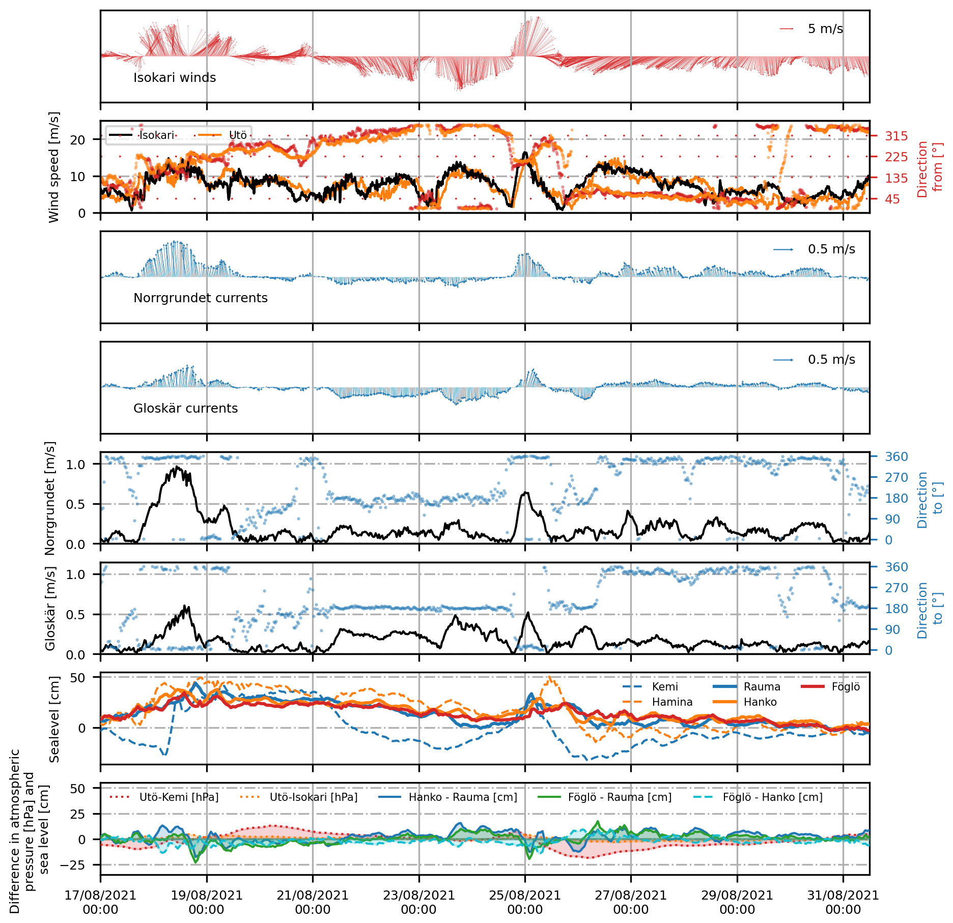
Figure A1 Time series of the Isokari winds and currents from Norrgrundet and Gloskär with simultaneous wind and sea level measurements, together with sea level and atmospheric pressure differences from the surrounding stations (Fig. 1). The first and second panels present the wind speed and direction at Isokari (and Utö, shown in orange in the second panel), and the third and fourth panels show currents in the uppermost layer measured at Norrgrundet and Gloskär. The upward arrow indicates the northward direction. The lowest panel shows the differences in sea level and atmospheric pressure around the AS.

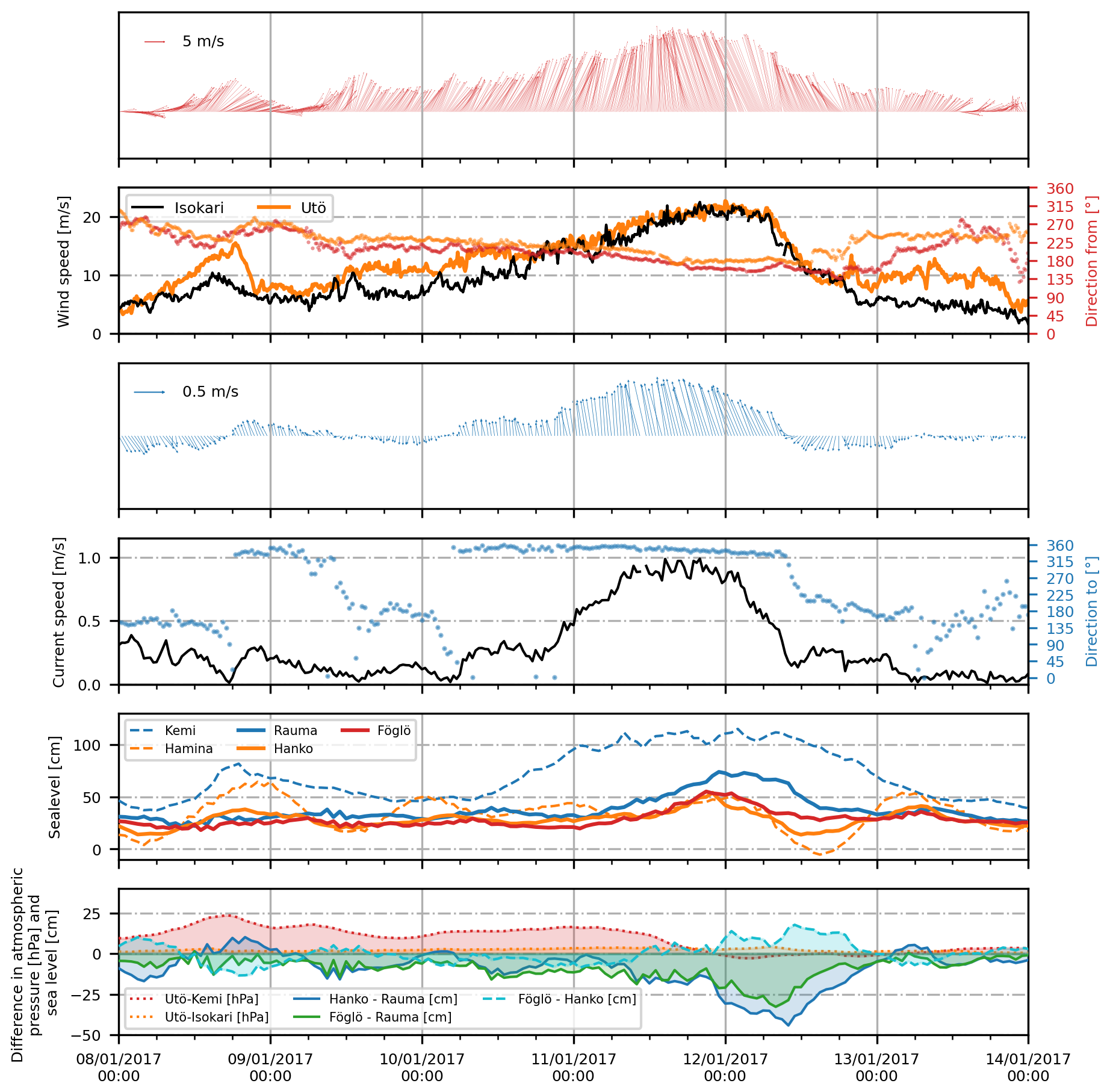
Figure A2 Time series of the third-strongest event of Norrgrundet currents (storm Toini on 11 January 2017) with simultaneous wind and sea level measurements, together with sea level and atmospheric pressure differences from the surrounding stations (Fig. 1). The first and second panels present the wind speed and direction at Isokari (and Utö, shown in orange in the second panel), and the third and fourth panels show currents in the uppermost layer measured at Norrgrundet. The upward arrow indicates the northward direction for the wind and current measurements. The fifth panel presents the sea level variation around the AS (solid lines) and at the end of the surrounding basins (dashed lines). The lowest panel shows the differences in sea level and atmospheric pressure fields around the AS.