Regional modeling of internal-tide dynamics around New Caledonia – Part 2: Tidal incoherence and implications for sea surface height observability

New Caledonia, in the southwestern tropical Pacific, has recently been identified as a hot spot for energetic semidiurnal internal tides. In a companion paper, the life cycle of coherent internal tides, characterized by fixed amplitude and phase, was investigated in the region through harmonic analysis of a year-long, hourly time series from numerical simulation output. In this study, we investigate the temporal variability of the internal tide by decomposing the semidiurnal signals into coherent and incoherent components. Semidiurnal barotropic-to-baroclinic energy conversion is largely governed by the coherent component (> 90 %), amplified by a factor of 3 to 7 from neap to spring tides through the interaction of M₂ and S₂ barotropic tidal currents. Incoherent conversion – negligible in the annual mean – can explain on monthly to intraseasonal scales a notable fraction of variability, modifying semidiurnal conversion by up to ±20 %. The latter is largely explained by local effects, particularly the work of the coherent barotropic tide on incoherent baroclinic bottom pressure amplitude variations, linked to mesoscale-eddy-induced stratification changes. Away from the generation sites, tidal incoherence increases, evident through altered orientation of tidal beams and increasing phase variability, caused mainly by interactions with mesoscale currents. Variations in conversion are not consistently proportional to those in energy flux divergence, suggesting that variations in energy dissipation are linked to additional mechanisms that deserve further investigation. The incoherent sea surface height signature, with a root mean square amplitude of 1–2 cm, is widespread across the domain and introduces limitations in disentangling balanced (near-geostrophic) and unbalanced (wave-like) motions in spectral space. Transition scales – the length scale at which unbalanced motions become dominant over balanced motions – are proven meaningful when inferred from altimetry tracks that align with the main propagation direction of internal tides. However, when not aligned the method is flawed as it does not take into account the anisotropy of internal-tide dynamics.

1 Introduction

Internal tides, i.e., internal waves at tidal frequency, are ubiquitous in the global ocean, where major bathymetric obstacles cause the energy transfer from the barotropic tide to baroclinic waves. These internal waves may either dissipate locally or propagate towards the open ocean: they are argued to play an essential role in our understanding of open-ocean mixing and the global oceanic energy budget (Melet et al., 2013; Waterhouse et al., 2014; Melet et al., 2016; de Lavergne et al., 2022). Well-known internal-tide generation sites for low vertical modes include Luzon Strait (e.g., Alford et al., 2011; Rainville et al., 2013; Kerry et al., 2016; Wang et al., 2023), the Hawaiian Ridge (e.g., Merrifield and Holloway, 2002; Carter et al., 2008; Zilberman et al., 2011), the Indonesian/Solomon seas (e.g., Nagai and Hibiya, 2015; Tchilibou et al., 2020), and the Amazonian Shelf Break (e.g., Tchilibou et al., 2022). From semi-analytical theory (Falahat et al., 2014b; de Lavergne et al., 2019; Vic et al., 2019), satellite altimetry (Ray and Zaron, 2016; Zhao et al., 2016; Zaron, 2019), and global numerical simulations (Müller et al., 2012; Shriver et al., 2012; Arbic, 2022; Buijsman et al., 2017), the southwestern tropical Pacific is also known to be an internal-tide generation hot spot but has not received particular attention until very recently (Bendinger et al., 2023, 2024).

Based on full-calendar-year, hourly regional simulation output, Bendinger et al. (2023, hereinafter Part 1) analyzed the internal-tide life cycle around New Caledonia, strongly dominated by the semidiurnal M₂ tide. They estimated 15.27 GW of energy converted from the barotropic to baroclinic tide, closely associated with the northwest–southeast-extending ridge system, continental slopes, shelf breaks, and seamounts. Over 50 % of this energy dissipates near generation sites, while the remainder propagates in tidal beams north and south of the island, with fluxes up to 30 kW m⁻¹. These energetics are comparable to other internal-tide generation hot spots in the Pacific such as Luzon Strait and the Hawaiian Ridge.

The above results are based on harmonic analysis representative of the phase-coherent tide only, with a fixed amplitude and phase that is predictable well in time and space through the astronomical tide forcing. Departures from tidal coherence, i.e., tidal incoherence, were not addressed, though global or basin-wide numerical simulation output suggests elevated levels of tidal incoherence, which can explain well above 50 % of the semidiurnal tidal variance (Buijsman et al., 2017; Nelson et al., 2019). The phase-incoherent tide can be understood as temporal variations of amplitude and phase within the tidal frequency band and is therefore mostly unpredictable (Nash et al., 2012; Kerry et al., 2013; Buijsman et al., 2017). It can represent an essential fraction of the total variance and an important contribution to the internal-tide life cycle (Zilberman et al., 2011; Buijsman et al., 2017; Zaron, 2017). As a consequence, internal-tide dissipation – estimated as the residual between local conversion and energy flux divergence and deduced in Part 1 – may have been overestimated as it contained both true baroclinic energy dissipation and energy transferred to the incoherent tide. In addition, some of the conclusions, such as those on sea surface height (SSH), should be revisited while considering the importance of tidal incoherence.

Sources of tidal incoherence are numerous and linked to interannual, seasonal, and mesoscale variability of stratification and background currents (Rainville and Pinkel, 2006; Tchilibou et al., 2020; Cai et al., 2024; Kaur et al., 2024). In the near field, i.e., close to internal-tide generation sites, local stratification changes or impinging remotely generated internal tides can induce barotropic-to-baroclinic conversion variations by altering the baroclinic bottom pressure (Kelly and Nash, 2010; Zilberman et al., 2011; Kerry et al., 2014; Pickering et al., 2015; Kerry et al., 2016). In the far field, i.e., away from the generation site and in the tidal energy propagation direction, tidal incoherence is commonly induced by spatiotemporal variations of stratification and background currents such as midlatitude and equatorial jets as well as the mesoscale eddy field (Park and Watts, 2006; Rainville and Pinkel, 2006; Dunphy and Lamb, 2014; Ponte and Klein, 2015; Kelly and Lermusiaux, 2016; Buijsman et al., 2017; Duda et al., 2018; Guo et al., 2023). The mechanisms governing temporal variability of the internal tide vary geographically and cannot be generalized as the importance of seasonality (among others) is not directly comparable across ocean basins. Further, temporal variations may be highly unpredictable, linked to mesoscale eddy variability. Quantifying these dynamics remains a challenge and demands dedicated regional studies. New Caledonia is a particularly challenging region as it is a hot spot of internal-tide generation and a region of strong mesoscale variability, making it subject to eddy–internal-tide interactions.

Whether tidal incoherence facilitates tidal energy dissipation is of current research interest. Generally, a loss of tidal coherence is not directly linked to tidal energy dissipation, but rather with nonlinear energy transfer to the incoherent tide, though it is often associated with energy being transferred from low to higher vertical modes with the latter tending to dissipate (Dunphy and Lamb, 2014; Bella et al., 2024). Wang and Legg (2023) showed that baroclinic eddies are capable of trapping low-mode internal tides and effectively transport energy to higher vertical modes, resulting in internal-tide dissipation within eddies. However, a robust estimate of the fraction of energy dissipation associated with such processes does not exist and may also vary geographically due to the different underlying dynamics. In turn, energy dissipation associated with the incoherent tide can have important implications for tidal mixing parameterizations in climate and ocean general circulation models, which do not resolve tidal processes. Current parameterizations rely heavily on semi-analytical theory, which do not take into account temporal variations of the background stratification and currents (Vic et al., 2019; de Lavergne et al., 2019, 2020). Further effort is therefore needed to quantify the internal-tide life cycle and energy dissipation.

Internal tides are of particular interest in the context of the Surface Water Ocean Topography (SWOT) satellite altimetry mission launched in December 2022, providing high-resolution SSH observations down to 15 km wavelength – an order of magnitude higher resolution than conventional satellite altimetry – for three main reasons (Fu and Ubelmann, 2014; Fu et al., 2024). First, SWOT will contribute to the characterization of the internal-tide SSH signature including those associated with higher vertical modes, which are associated with shorter horizontal scales than low vertical modes (Arbic et al., 2018). Second, combined SSH observations of balanced and unbalanced motions allow us to study nonlinear scale interactions down to submesoscales and will eventually help us understand the energy transfer toward dissipation scales on global scales (Klein et al., 2019; Morrow et al., 2019). Third, accurate knowledge of the internal-tide SSH signature is crucial for the study of mesoscale and submesoscale dynamics. In other words, the extent to which we can exploit SWOT's potential to study fine-scale oceanic dynamics depends on our ability to disentangle the measured SSH signal associated with balanced and unbalanced motions, i.e., mesoscale to submesoscale dynamics and internal gravity waves. In this regard, the transition scale typically serves as a quantity to estimate the length scale L_t at which unbalanced motions become dominant over balanced motions (Vergara et al., 2023), though this is problematic in regions where balanced and unbalanced motions feature equal SSH variance at similar wavelengths (Callies and Wu, 2019). A correction for the coherent internal tide partially addresses this problem while increasing SSH observability of mesoscale to submesoscale dynamics (Qiu et al., 2018; Carrere et al., 2021; Arbic, 2022). The High-Resolution Empirical Tide (HRET) model derived from over 20-year-long altimeter time series is currently used to apply such correction (Zaron, 2019). However, this correction does not consider incoherent internal tides that can explain a large fraction of the total SSH variance (Zaron, 2017; Lahaye et al., 2024). This makes the dynamical interpretation of SWOT SSH, i.e., the allocation of different dynamics to SSH, a difficult challenge in regions where tidal incoherence is important.

The objective of the presented study is to (1) identify regions of important tidal incoherence around New Caledonia, (2) quantify its relative importance across different timescales, and (3) understand the underlying mechanisms leading to tidal incoherence. What are the processes, in both the near and far field, that drive temporal variability in the barotropic-to-baroclinic conversion term and the propagation of energy? Finally, (4) how does the incoherent tide manifest in SSH, and what are the potential implications for SSH observability of balanced motions in the southwestern tropical Pacific?

The study is organized as follows. In Sect. 2, we give a description of the regional numerical model configuration, previously introduced in Part 1, as well as the underlying methodology used to infer temporal variability of the internal tide. In Sect. 3, we begin with an analysis of the semidiurnal tidal diagnostics, decomposed into their coherent and incoherent components. We then discuss in greater detail how mesoscale eddy variability drives temporal variability in the barotropic-to-baroclinic conversion term (Sect. 4) and energy flux (Sect. 5). In Sect. 6 we address the importance of the incoherent SSH signature around New Caledonia and what implications it can have for SSH observability of mesoscale to submesoscale dynamics. We finish with a summary and perspectives of this work in Sect. 7.

2 Data and methods

2.1 Numerical simulation

We use a regional model configuration that consists of a host grid (TROPICO12, $\mathrm{1}/\mathrm{12}$° horizontal resolution and 125 vertical levels) that covers the tropical and subtropical Pacific Ocean basin from 142° E–70° W and 46° S–24° N, introduced in Part 1. The oceanic reanalysis GLORYS2V4 prescribes initial conditions for temperature and salinity as well as the forcing with daily currents, temperature, and salinity at the open lateral boundaries. ERA5 produced by the European Centre for Medium-Range Weather Forecasts (ECMWF, Hersbach et al., 2020) provides atmospheric forcing at hourly temporal resolution and a spatial resolution of $\mathrm{1}/\mathrm{4}$° to compute surface fluxes using bulk formulae and the model prognostic sea surface temperature. The model is forced by the tidal potential of the five major diurnal (K1, O1) and semidiurnal (M₂, S₂, N₂) tidal constituents. At the open lateral boundaries it is forced by barotropic SSH and barotropic currents of the same five tidal constituents taken from the global tide atlas FES2014 (Finite Element Solution 2014, Lyard et al., 2021).

We build on hourly numerical simulation outputs from a higher-resolution horizontal grid refinement within the host grid in the southwestern tropical Pacific Ocean encompassing New Caledonia (CALEDO60). This nesting grid features $\mathrm{1}/\mathrm{60}$° horizontal resolution or ∼ 1.7 km grid spacing initialized by Adaptive Grid Refinement in Fortran (AGRIF, Debreu et al., 2008). Specifically, we make use of the three-dimensional velocity, temperature, salinity, and pressure fields as well as SSH. Coherent tidal harmonics are taken from Part 1 based on harmonic analysis and vertical mode decomposition. We refer the reader to Sect. 2.2 in Part 1 for more details. Both full-model variables and tidal harmonics are constrained to a full calendar year (model year 2014). Constraining the analysis to a full calendar year relies upon a compromise between high computational expenses and a time series long enough for a robust extraction of the coherent tide.

The model's capability to realistically simulate ocean dynamics that range from the large-scale circulation down to high-frequency motion using climatology, satellite altimetry, and in situ measurements was addressed in Part 1. Regarding the dominant semidiurnal M₂ internal tide, confidence in the model's SSH signature is explicitly given by comparison with HRET, revealing reasonable amplitude and large-scale (interference) patterns (see Fig. 13a–d in Part 1). Furthermore, glider observations revealed the model's accurate representation of the spatiotemporal variability of the semidiurnal energy flux south of New Caledonia, including the location, magnitude, and vertical structure/extent of the westward internal-tide energy propagation characterized by narrow tidal beams (Bendinger et al., 2024).

2.2 Tidal analysis and diagnostics

Similarly to Part 1, the internal-tide life cycle, i.e., internal-tide generation, propagation, and dissipation, is studied using the depth-integrated baroclinic energy equation (Simmons et al., 2004; Carter et al., 2008; Buijsman et al., 2017):

$$\begin{array}{}\text{(1)}& {\mathbf{\nabla }}_{\mathrm{h}}\cdot {\mathit{F}}_{\mathrm{bc}}-C+D_{\mathrm{bc}}=\mathrm{0},\end{array}$$

where ∇_h⋅F_bc is the baroclinic energy flux divergence with ∇_h the horizontal gradient operator and ${\mathit{F}}_{\mathrm{bc}}=(F_x,F_y)$ the energy flux vector, C is the barotropic-to-baroclinic conversion term, and D_bc is the baroclinic energy dissipation. D_bc is computed as the residual of ∇_h⋅F_bc and C. Further, we neglect the tendency of the total energy, i.e., $\partial /\partial t\left({\int }_{-H}^{\mathrm{0}}({\mathrm{KE}}_{\mathrm{bc}}+\mathrm{APE})\mathrm{d}z\right)$, where KE_bc is the baroclinic kinetic energy and APE available potential energy. Furthermore, F_bc consists only of contributions from hydrostatic pressure work, omitting contributions from KE and APE advection, nonhydrostatic pressure work, and diffusion (Kang and Fringer, 2012; Lahaye et al., 2020). These simplifications were made since the given terms were found to be negligibly small in the above studies when averaged over a set of tidal periods.

In Part 1, we estimated the coherent M₂ internal-tide energy budget based on a harmonic analysis referenced to a full model calendar year. Here, in Part 2, our major objective is to deduce time variability from Eq. (1) for the semidiurnal frequency band (^D2, 10–14 h) through a bandpass-filtering technique following Nash et al. (2012), Pickering et al. (2015), and Buijsman et al. (2017). Specifically, time variability is inferred by decomposing the bandpass-filtered contribution in Eq. (1) into the coherent (^coh) and incoherent (^inc) parts for the horizontal velocity vector u and the pressure perturbation p:

$$\begin{array}{}\text{(2)}& {\mathit{u}}^{\mathrm{D}\mathrm{2}}={\mathit{u}}^{\mathrm{coh}}+{\mathit{u}}^{\mathrm{inc}},p^{\mathrm{D}\mathrm{2}}=p^{\mathrm{coh}}+p^{\mathrm{inc}}.\end{array}$$

u^D2 and p^D2 can be further decomposed into their barotropic (_bt) and baroclinic (_bc) parts. The former is estimated by the depth average and the latter by the departure from the barotropic depth average:

$$\begin{array}{}\text{(3)}& \begin{array}{rl}& {\mathit{u}}_{\mathrm{bc}}^{\mathrm{D}\mathrm{2}}={\mathit{u}}^{\mathrm{D}\mathrm{2}}-\underset{{\mathit{u}}_{\mathrm{bt}}^{\mathrm{D}\mathrm{2}}}{\underbrace{{\displaystyle \frac{\mathrm{1}}{H}}\underset{-H}{\overset{\mathit{\eta }}{\int }}{\mathit{u}}^{\mathrm{D}\mathrm{2}}\mathrm{d}z}},\\ & p_{\mathrm{bc}}^{\mathrm{D}\mathrm{2}}=p^{\mathrm{D}\mathrm{2}}-\underset{p_{\mathrm{bt}}^{\mathrm{D}\mathrm{2}}}{\underbrace{{\displaystyle \frac{\mathrm{1}}{H}}\underset{-H}{\overset{\mathit{\eta }}{\int }}{p}^{\mathrm{D}\mathrm{2}}\mathrm{d}z}},\end{array}\end{array}$$

where H is the water column depth. The semidiurnal conversion term C^D2 can then be written as

$$\begin{array}{}\text{(4)}& {\displaystyle }{C}^{\mathrm{D}\mathrm{2}}={\displaystyle \frac{\mathrm{1}}{T}}\underset{T}{\int }-{\mathbf{\nabla }}_{\mathrm{h}}H\cdot {\mathit{u}}_{\mathrm{bt}}^{\mathrm{D}\mathrm{2}}{p}_{\mathrm{bc}}^{\mathrm{D}\mathrm{2}}(-H)\mathrm{d}t\text{(5)}& {\displaystyle }\begin{array}{rl}& ={\displaystyle \frac{\mathrm{1}}{T}}\underset{T}{\int }\underset{C^{\mathrm{coh}}}{\underbrace{(-{\mathbf{\nabla }}_{\mathrm{h}}H\cdot {\mathit{u}}_{\mathrm{bt}}^{\mathrm{coh}}{p}_{\mathrm{bc}}^{\mathrm{coh}}(-H)}}\\ & \underset{C^{\mathrm{inc}}}{\underbrace{\underset{C^{{\mathrm{inc}}^{*}}}{\underbrace{-{\mathbf{\nabla }}_{\mathrm{h}}H\cdot {\mathit{u}}_{\mathrm{bt}}^{\mathrm{inc}}{p}_{\mathrm{bc}}^{\mathrm{inc}}(-H)}}\underset{C^{\mathrm{cross}}}{\underbrace{-{\mathbf{\nabla }}_{\mathrm{h}}H\cdot {\mathit{u}}_{\mathrm{bt}}^{\mathrm{coh}}{p}_{\mathrm{bc}}^{\mathrm{inc}}(-H)-{\mathbf{\nabla }}_{\mathrm{h}}H\cdot {\mathit{u}}_{\mathrm{bt}}^{\mathrm{inc}}{p}_{\mathrm{bc}}^{\mathrm{coh}}(-H)}}}})\mathrm{d}t,\end{array}\end{array}$$

decomposed into the coherent (C^coh) and incoherent conversion ($C^{\mathrm{inc}}=C^{{\mathrm{inc}}^{*}}+C^{\mathrm{cross}}$), averaged over a given time period T. Using least-squares fitting to extract the coherent component, the cross-terms $C^{\mathrm{cross}}=C^{\mathrm{cross}\mathrm{1}}+C^{\mathrm{cross}\mathrm{2}}$, where $C^{\mathrm{cross}\mathrm{1}}=-{\mathbf{\nabla }}_{\mathrm{h}}H\cdot {\mathit{u}}_{\mathrm{bt}}^{\mathrm{coh}}{p}_{\mathrm{bc}}^{\mathrm{inc}}(-H)$ and $C^{\mathrm{cross}\mathrm{2}}=-{\mathbf{\nabla }}_{\mathrm{h}}H\cdot {\mathit{u}}_{\mathrm{bt}}^{\mathrm{inc}}{p}_{\mathrm{bc}}^{\mathrm{coh}}(-H)$, are, by construction, considered incoherent. This classification follows from the orthogonality condition inherent in the least-squares framework: the residual (i.e., the incoherent component) is uncorrelated with the fitted coherent signal and lacks a consistent phase relationship with the tidal forcing. In other words, there is no preferred phasing between coherent and incoherent motions. As a consequence, bilinear products between coherent and incoherent fields tend to average out or remain negligibly small over the regression interval (Nash et al., 2012; Buijsman et al., 2017; Savage et al., 2020). However, as we show in the analysis below, these cross-terms can account for a substantial fraction of the variability on shorter timescales. We specifically focus on assessing their relative importance to better understand temporal variations in the conversion term and the physical mechanisms that drive them.

Similarly to C^D2, the semidiurnal depth-integrated energy flux ${\mathit{F}}_{\mathrm{bc}}^{\mathrm{D}\mathrm{2}}$ can be written as

$$\begin{array}{}\text{(6)}& {\displaystyle }{\mathit{F}}_{\mathrm{bc}}^{\mathrm{D}\mathrm{2}}={\displaystyle \frac{\mathrm{1}}{T}}\underset{T}{\int }\underset{-H}{\overset{\mathit{\eta }}{\int }}{\mathit{u}}_{\mathrm{bc}}^{\mathrm{D}\mathrm{2}}{p}_{\mathrm{bc}}^{\mathrm{D}\mathrm{2}}\mathrm{d}z\mathrm{d}t\text{(7)}& {\displaystyle }={\displaystyle \frac{\mathrm{1}}{T}}\underset{T}{\int }\underset{{\mathit{F}}_{\mathrm{bc}}^{\mathrm{coh}}}{\underbrace{(\underset{-H}{\overset{\mathit{\eta }}{\int }}{\mathit{u}}_{\mathrm{bc}}^{\mathrm{coh}}{p}_{\mathrm{bc}}^{\mathrm{coh}}\mathrm{d}z}}+\underset{{\mathit{F}}_{\mathrm{bc}}^{\mathrm{inc}}}{\underbrace{\underset{-H}{\overset{\mathit{\eta }}{\int }}({\mathit{u}}_{\mathrm{bc}}^{\mathrm{inc}}{p}_{\mathrm{bc}}^{\mathrm{inc}}+{\mathit{u}}_{\mathrm{bc}}^{\mathrm{coh}}{p}_{\mathrm{bc}}^{\mathrm{inc}}+{\mathit{u}}_{\mathrm{bc}}^{\mathrm{inc}}{p}_{\mathrm{bc}}^{\mathrm{coh}})\mathrm{d}z}})\mathrm{d}t.\end{array}$$

The coherent terms ${\mathit{u}}_{\mathrm{bt}}^{\mathrm{coh}}$, ${\mathit{u}}_{\mathrm{bc}}^{\mathrm{coh}}$, and $p_{\mathrm{bc}}^{\mathrm{coh}}$ are taken from the harmonic analysis and vertical mode decomposition carried out in Part 1. Here, they are representative of the semidiurnal frequency band including the M₂, S₂, and N₂ tidal frequencies. The barotropic part is equivalent to mode 0 and the baroclinic part to the sum of modes 1–9. The incoherent terms are computed as the difference between the above semidiurnal bandpassed and coherent time series, i.e.,

$$\begin{array}{}\text{(8)}& \begin{array}{rl}& {\mathit{u}}_{\mathrm{bt}}^{\mathrm{inc}}={\mathit{u}}_{\mathrm{bt}}^{\mathrm{D}\mathrm{2}}-{\mathit{u}}_{\mathrm{bt}}^{\mathrm{coh}},{\mathit{u}}_{\mathrm{bc}}^{\mathrm{inc}}={\mathit{u}}_{\mathrm{bc}}^{\mathrm{D}\mathrm{2}}-{\mathit{u}}_{\mathrm{bc}}^{\mathrm{coh}},\\ & p_{\mathrm{bc}}^{\mathrm{inc}}=p_{\mathrm{bc}}^{\mathrm{D}\mathrm{2}}-p_{\mathrm{bc}}^{\mathrm{coh}}.\end{array}\end{array}$$

Semidiurnal energy dissipation $D_{\mathrm{bc}}^{\mathrm{D}\mathrm{2}}$ is defined as

$$\begin{array}{}\text{(9)}& {\displaystyle }{D}_{\mathrm{bc}}^{\mathrm{D}\mathrm{2}}={\displaystyle \frac{\mathrm{1}}{T}}\underset{T}{\int }(-{\mathbf{\nabla }}_{\mathrm{h}}\cdot {\mathit{F}}_{\mathrm{bc}}^{\mathrm{D}\mathrm{2}}+C^{\mathrm{D}\mathrm{2}})\mathrm{d}t\text{(10)}& {\displaystyle }\begin{array}{rl}& ={\displaystyle \frac{\mathrm{1}}{T}}\underset{T}{\int }\left(\underset{D_{\mathrm{bc}}^{\mathrm{coh}}}{\underbrace{-{\mathbf{\nabla }}_{\mathrm{h}}\cdot {\mathit{F}}_{\mathrm{bc}}^{\mathrm{coh}}+C^{\mathrm{coh}}}}\right)\mathrm{d}t\\ & +{\displaystyle \frac{\mathrm{1}}{T}}\underset{T}{\int }\left(\underset{D_{\mathrm{bc}}^{\mathrm{inc}}}{\underbrace{-{\mathbf{\nabla }}_{\mathrm{h}}\cdot {\mathit{F}}_{\mathrm{bc}}^{\mathrm{inc}}+C^{\mathrm{inc}}}}\right)\mathrm{d}t.\end{array}\end{array}$$

An important conclusion concerning the coherent internal-tide analysis in Part 1 was that $D_{\mathrm{bc}}^{\mathrm{coh}}$ may not be associated entirely with true energy dissipation. In fact, $D_{\mathrm{bc}}^{\mathrm{coh}}$ represents both energy dissipation and energy transfer to the incoherent tide. It also includes the energy transfer to higher harmonics (higher-frequency waves), which, however, is presumably expressed in numerical dissipation due to spatial resolution constraints (Peacock and Tabaei, 2005; Zeng et al., 2021). While $D_{\mathrm{bc}}^{\mathrm{D}\mathrm{2}}$ accounts for actual energy dissipation, $D_{\mathrm{bc}}^{\mathrm{inc}}$ consists of both the fraction by which $D_{\mathrm{bc}}^{\mathrm{coh}}$ is mistakenly associated with true energy dissipation (or the error by which energy dissipation in $D_{\mathrm{bc}}^{\mathrm{coh}}$ is overestimated) and incoherent energy dissipation.

2.3 Ray tracing

A ray-tracing method following Rainville and Pinkel (2006) is employed, which models the horizontal propagation of internal gravity wave modes in the presence of spatially varying topography, planetary vorticity, stratification, and depth-averaged currents. Here, the objective is to interpret the tidal beam's departure from tidal coherence in the far field, attributed to the refraction by mesoscale eddies. Specifically, we model semidiurnal ray paths for the first baroclinic mode for monthly varying stratification and currents. Note that the choice of depth-averaged currents is simplistic and relies on the assumption that vertically sheared background currents associated with mesoscale eddies do not alter the qualitative picture of ray trajectories that are obtained. To distinguish between mesoscale stratification and current effects, we consider three different scenarios: (1) monthly varying stratification and currents, (2) monthly varying stratification and annually averaged currents, and (3) annually averaged stratification and monthly varying currents. The reference ray path is given by annually averaged stratification and currents, representative of tidal coherence.

Internal gravity wave speeds are solved by the Sturm–Liouville problem for given stratification and bathymetry from CALEDO60. The semidiurnal rays are initialized at 167.75° E, 18.4° S and 167.65° E, 23.35° S within the two major internal-tide generation hot spots as identified in Part 1, i.e., the North (1) and South (2) domains (see Fig. 1), and for a given propagation angle: northeastward (45°) and southwestward (210°), respectively. In an iterative procedure, the ray tracing considers for each step size (1 km) bathymetry, planetary vorticity effects, stratification, and currents.

3 Annual mean of semidiurnal, coherent, and incoherent tidal diagnostics

The depth-integrated semidiurnal barotropic-to-baroclinic conversion, energy flux, and dissipation (residual) were computed for a full model calendar year in the whole domain, decomposed into the coherent and incoherent components (see Sect. 2.2). The annual mean is shown in Fig. 1. In Part 1, we identified four hot-spot regions of internal-tide generation: North (1), South (2), Norfolk Ridge (3), and Loyalty Ridge (4) (see Fig. 1). Integrated over the subdomains, the barotropic-to-baroclinic conversion is almost entirely dominated by the coherent component (Fig. 1a–b, Table 1). The incoherent component is negligible (Fig. 1c). However, we will show in Sect. 4 that on shorter timescales the conversion term is subject to temporal variations not linked to the astronomical tide forcing.

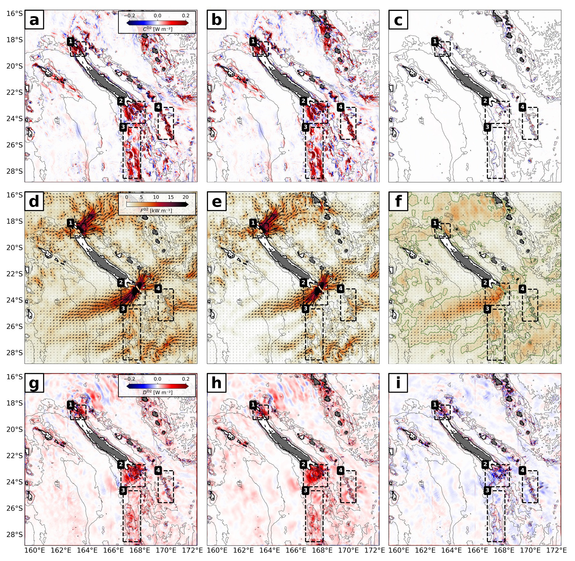
Figure 1 Annual mean, depth-integrated, semidiurnal (a) barotropic-to-baroclinic energy conversion, decomposed into the (b) coherent and (c) incoherent components. Panels (d)–(f) and (g)–(i) are the same as (a)–(c) but for the depth-integrated, semidiurnal energy flux and dissipation (residual), respectively. For the incoherent energy flux (f), the 2 kW m⁻¹ contour is also shown. The thin black lines represent the 1000, 2000, and 3000 m depth contours. The thick black line is the 100 m depth contour representative of the New Caledonian lagoon. The numbered black boxes represent the hot spots of internal-tide generation (1: North, 2: South, 3: Norfolk Ridge, 4: Loyalty Ridge).

As stated in Part 1, the depth-integrated energy flux is characterized in the annual mean by two tidal beams that emerge and diverge from the North (1) and South (2) domains (Fig. 1d). While the coherent component is dominant, the incoherent component does explain an important fraction (Fig. 1e–f). This is particularly the case for the South (2) and Loyalty Ridge (4) domains, where the area-integrated incoherent energy flux divergence accounts for roughly 13 % and 16 % of the semidiurnal energy flux divergence, respectively (Table 1). In the North (1) and Norfolk Ridge (3) domains, it accounts for roughly 4 %. Outside and with increasing distance from the generation sites, i.e., in the far field, $\left|{\mathit{F}}_{\mathrm{bc}}^{\mathrm{inc}}\right|$ becomes more important with ratios $\left|{\mathit{F}}_{\mathrm{bc}}^{\mathrm{inc}}\right|/\left|{\mathit{F}}_{\mathrm{bc}}^{\mathrm{D}\mathrm{2}}\right|$ = 0.5–0.9 (not shown). However, it is important to note that in these cases $\left|{\mathit{F}}_{\mathrm{bc}}^{\mathrm{D}\mathrm{2}}\right|$ is considerably reduced (< 5 kW m⁻¹).

The residual $D_{\mathrm{bc}}^{\mathrm{D}\mathrm{2}}$ is here taken as a proxy for energy dissipation following the discussion in Sect. 2.2. Integrated over the subdomains North (1), South (2), Norfolk Ridge (3), and Loyalty Ridge (4), 38 %, 58 %, 40 %, and 29 % of the locally generated energy is dissipated in the near field, respectively (Fig. 1g, Table 1). $D_{\mathrm{bc}}^{\mathrm{coh}}$ is representative of both coherent energy dissipation and energy being removed from the coherent internal tide through nonlinear energy transfers (Fig. 1h). $D_{\mathrm{bc}}^{\mathrm{inc}}$ consists of incoherent energy dissipation and energy transferred from the coherent tide to the incoherent tide. The latter is expressed by net negative ratios of $D_{\mathrm{bc}}^{\mathrm{inc}}$ and $D_{\mathrm{bc}}^{\mathrm{coh}}$ and accounts for 10 %, 9 %, and 22 % in the South (2), Norfolk Ridge (3), and Loyalty Ridge (4) domains, respectively (Fig. 1i and Table 1). These ratios are equivalent to the fraction by which energy dissipation is overestimated in $D_{\mathrm{bc}}^{\mathrm{coh}}$. In the North (1) domain, $D_{\mathrm{bc}}^{\mathrm{inc}}$ is slightly positive (3 %), suggesting net energy dissipation linked to the incoherent tide.

Table 1 Annual mean and standard deviation of the regional semidiurnal barotropic-to-baroclinic conversion C^D2, baroclinic energy flux divergence ${\mathbf{\nabla }}_{\mathrm{h}}\cdot {\mathit{F}}_{\mathrm{bc}}^{\mathrm{D}\mathrm{2}}$, and baroclinic dissipation $D_{\mathrm{bc}}^{\mathrm{D}\mathrm{2}}$ integrated over the North (1), South (2), Norfolk Ridge (3), and Loyalty Ridge (4) domains and decomposed into their coherent and incoherent parts.

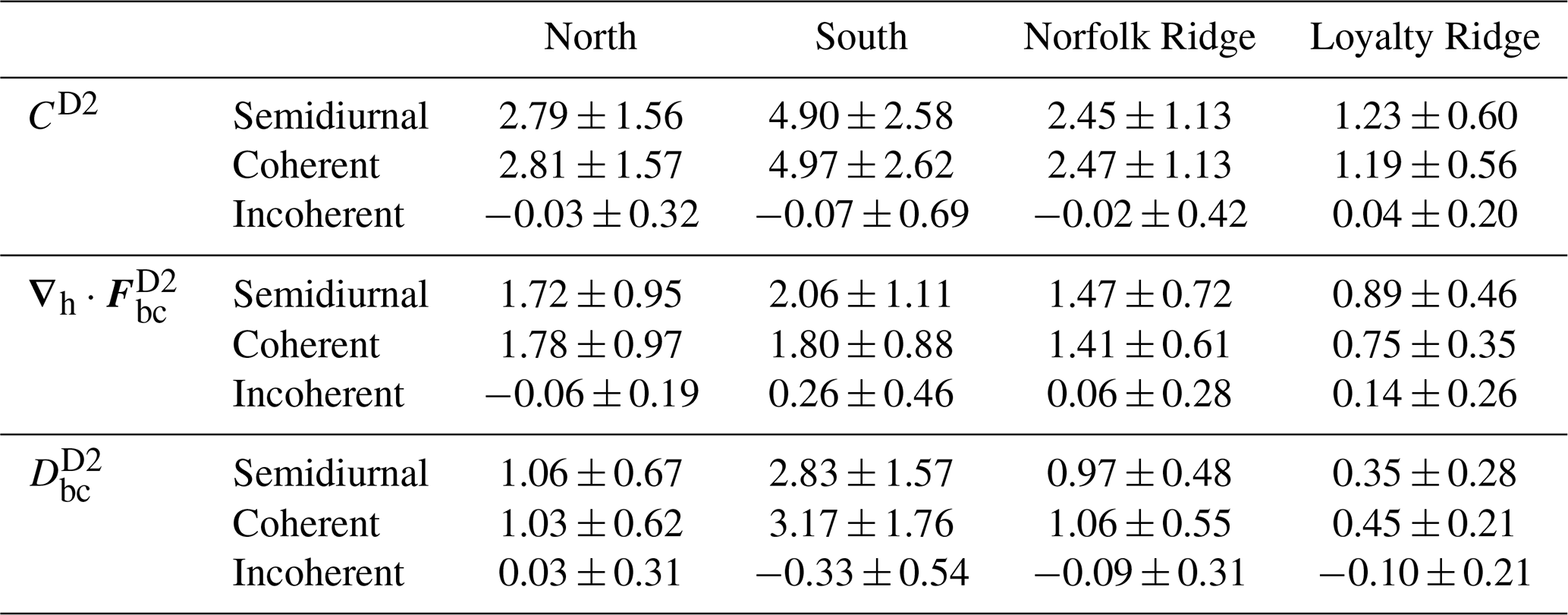
All units are given in GW.

4 What drives semidiurnal barotropic-to-baroclinic energy conversion variability?

4.1 Coherent vs. incoherent contributions

In the annual mean, the semidiurnal barotropic-to-baroclinic conversion is largely dominated by the coherent component. Meanwhile, it is the coherent tide that is associated with a substantial amount of variability due to the spring–neap cycle, driven by the interaction of M₂ and S₂ tidal constituents (Fig. 2). Note that the N₂ tidal constituent adds a low-frequency component to the modeled variability with a period of ∼ 9 months. Specifically, on timescales of ∼ 2 weeks conversion linked to the coherent tide may vary on average by a factor which ranges between 3 and 7 among the subdomains between spring and neap tides. This is in agreement with recent findings over the Reykjanes Ridge (Vic et al., 2021). The coherent conversion explains in the area integral most of the semidiurnal variability (γ^coh= 0.90–0.99) within the internal-tide generation hot spots (Table 2). The remaining fraction is explained by the incoherent tide (γ^inc= 0.01–0.10).

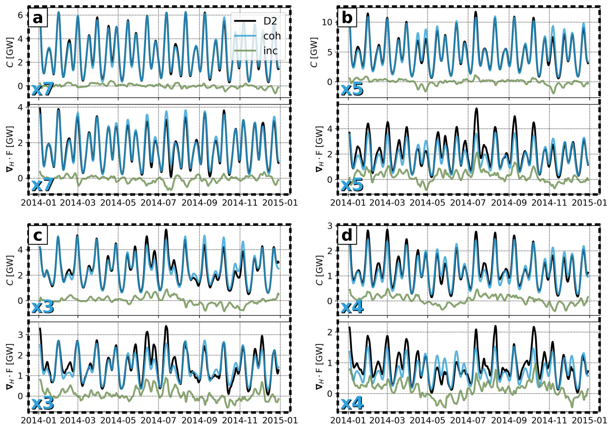
Figure 2 Time series of semidiurnal (black) barotropic-to-baroclinic conversion C^D2 and energy flux divergence ${\mathbf{\nabla }}_{\mathrm{h}}\cdot {\mathit{F}}_{\mathrm{bc}}^{\mathrm{D}\mathrm{2}}$, decomposed into the coherent (blue) and incoherent (green) components, integrated over (a) North, (b) South, (c) Norfolk Ridge, and (d) Loyalty Ridge. The mean factor of change for C^coh and ${\mathbf{\nabla }}_{\mathrm{h}}\cdot {\mathit{F}}_{\mathrm{bc}}^{\mathrm{coh}}$ between spring and neap tides (∼ 2 weeks) is also given (in blue in the lower left corner).

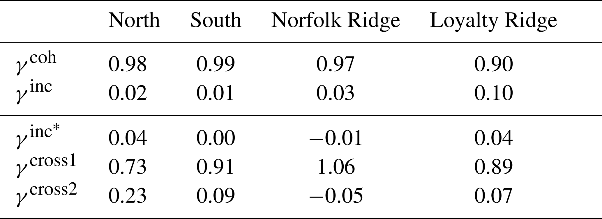
Table 2 Domain-averaged explained variance of the coherent (${\mathit{\gamma }}^{\mathrm{coh}}=\mathrm{cov}(C^{\mathrm{coh}},C^{\mathrm{D}\mathrm{2}})/\mathrm{var}\left(C^{\mathrm{D}\mathrm{2}}\right))$) and incoherent (γ^inc) barotropic-to-baroclinic conversion referenced to the semidiurnal conversion variability (C^D2). The domain-averaged explained variability of the purely incoherent term ${\mathit{\gamma }}^{{\mathrm{inc}}^{*}}=\mathrm{cov}(C^{{\mathrm{inc}}^{*}},C^{\mathrm{inc}})/\mathrm{var}\left(C^{\mathrm{inc}}\right))$) and the two cross-terms (γ^cross1, γ^cross2) relative to the incoherent conversion variability (C^inc) is also given. We refer to Eq. (5) for the decomposition of C^D2 and C^inc.

We explicitly show the spatial contribution to semidiurnal conversion variability by the coherent and incoherent parts for the South (2) domain (Fig. 3). The South (2) domain represents the most prominent internal-tide generation site with conversion rates well above 1 W m⁻² across steep slopes such as Pines Ridge (Fig. 3a). Even though it is the coherent tide and, thus, the spring–neap cycle which dominate semidiurnal variability, certain regions stand out with increasing contributions of the incoherent tide (C^inc). This is the case close to the lagoon and to the southeast around seamounts, notably Antigonia, Jumeaux Est, Jumeaux Ouest, and Stylaster (Fig. 3c). In these regions, the incoherent tide can explain well above 50 % of the semidiurnal conversion variability. However, it is worth mentioning that they are generally associated with reduced values of C^D2 compared to the overwhelmingly strong generation at Pines Ridge. This is crucial knowledge for the design and interpretation of in situ observations at fixed locations such as moorings (see Sect. 7).

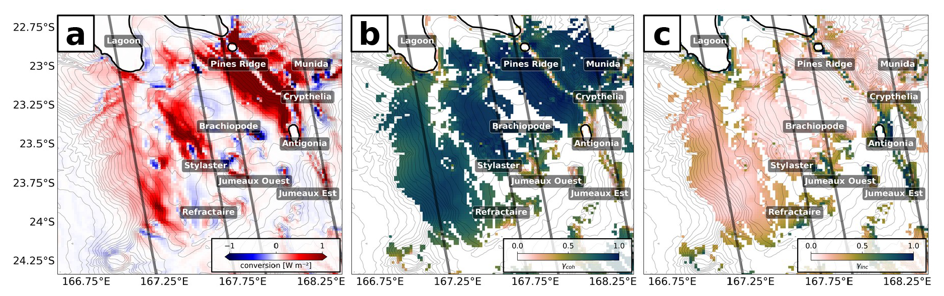
Figure 3 (a) Annual mean, depth-integrated, semidiurnal barotropic-to-baroclinic energy conversion as in Fig. 1a, but zoomed into the South (2) domain. Explained variance is shown for the (b) coherent (${\mathit{\gamma }}^{\mathrm{coh}}=\mathrm{cov}(C^{\mathrm{coh}},C^{\mathrm{D}\mathrm{2}})/\mathrm{var}\left(C^{\mathrm{D}\mathrm{2}}\right)$) and (c) incoherent (${\mathit{\gamma }}^{\mathrm{inc}}=\mathrm{cov}(C^{\mathrm{inc}},C^{\mathrm{D}\mathrm{2}})/\mathrm{var}\left(C^{\mathrm{D}\mathrm{2}}\right)$) component. Explained variance is only shown for regions where $\left|C^{\mathrm{D}\mathrm{2}}\right|>$ 0.05 W m⁻². The depth contour interval is 100 m. The SWOT swaths (solid black lines) during the fast sampling phase (1 d repeat orbit) are also shown.

To better understand the origin of C^inc, we further decompose it into a purely incoherent term ($C^{{\mathrm{inc}}^{*}}$) and two cross-terms (C^cross1, C^cross2) following Eq. (5). Across all internal-tide generation hot spots, C^cross1 dominates (γ^cross1>  0.73; Table 2). This implies that semidiurnal conversion variability (apart from the tidal-forcing-induced spring–neap variability) is driven by the work of the coherent barotropic tide on incoherent baroclinic bottom pressure variations $p_{\mathrm{bc}}^{\mathrm{inc}}(-H)$. C^cross2, linked to temporal variations of the barotropic forcing, can account for up to γ^cross2= 0.23. $C^{{\mathrm{inc}}^{*}}$ tends to play a negligible role. We note that $C^{{\mathrm{inc}}^{*}}$ and C^cross2 can have compensating effects (see Norfolk Ridge (3) in Table 2), but the mechanisms underlying this compensation remain unclear.

Similarly to the analysis above, we show for the South (2) domain the contribution of the different terms that make up C^inc (Fig. 4). The annual means for $C^{{\mathrm{inc}}^{*}}$, C^cross1, and C^cross2 are shown in Fig. 4a–c. Note that the color bar range is an order of magnitude smaller than in Fig. 1a–c and that the overall contribution to the annual mean remains small. While the three terms feature similar amplitudes, their spatial patterns differ. Based on the area-integrated explained variance in Table 2 (γ^cross1= 0.91), alongside high standard deviations, C^cross1 dominates C^inc (Fig. 4e, h). C^cross2 plays a minor but non-negligible role (γ^cross1= 0.09) in the incoherent variance, with an elevated contribution particularly above steep bathymetry (Fig. 4f, i).

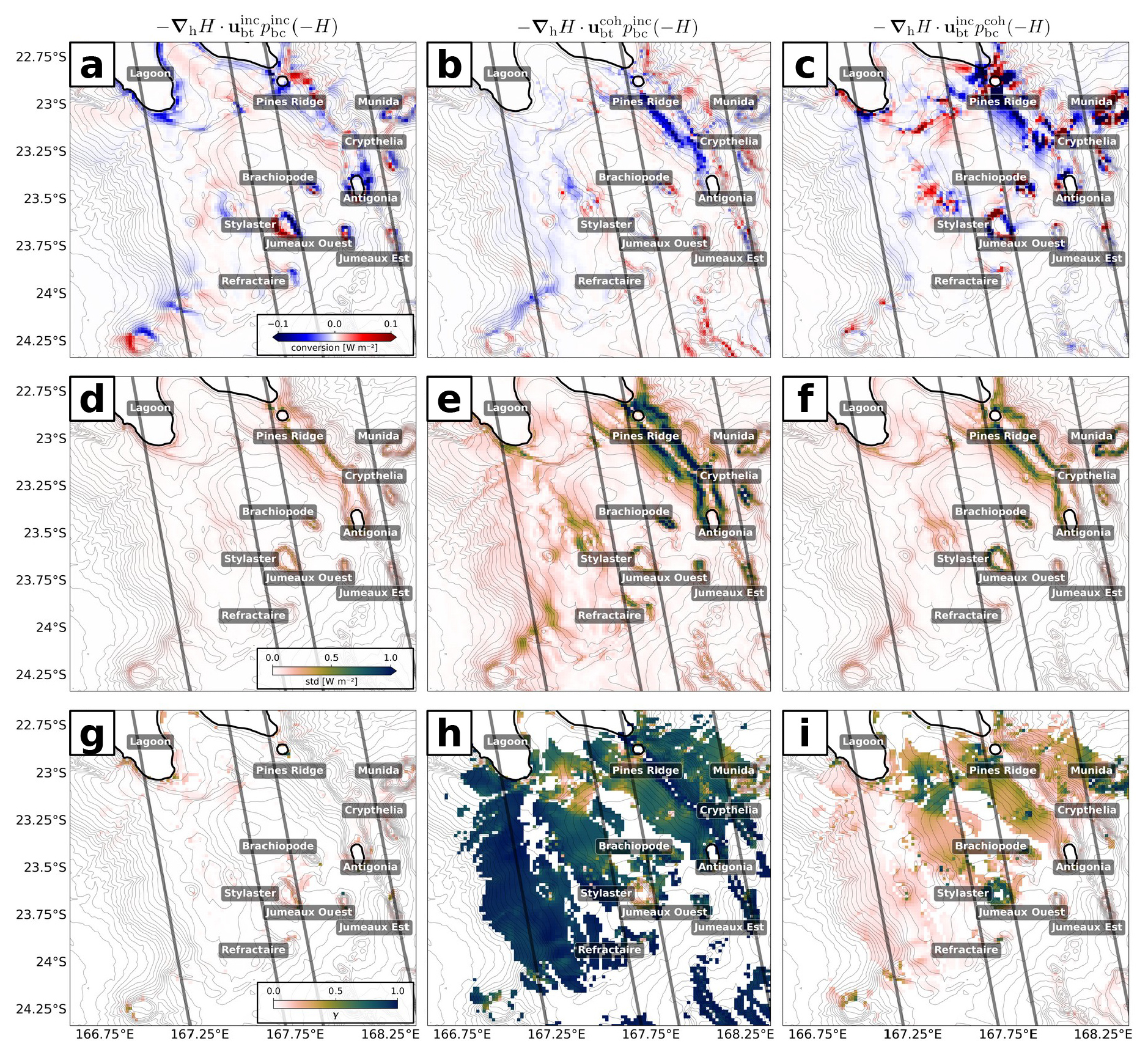
Figure 4 Annual mean and standard deviation of depth-integrated semidiurnal barotropic-to-baroclinic incoherent energy conversion separated into the (a, d) purely incoherent ($C^{{\mathrm{inc}}^{*}}$) term and the (b, e) first (C^cross1) and (c, f) second (C^cross2) cross-terms. The explained variabilities of (g) $C^{{\mathrm{inc}}^{*}}$, (h) C^cross1, and (i) C^cross2 are referenced to the incoherent conversion C^inc.

To summarize, incoherent conversion averages approximately to zero in the annual mean. Temporally, though, it features marked positive and negative contributions to the semidiurnal conversion at shorter timescales (see Fig. 2). Decomposing C^inc allows for a more detailed view of the origin of conversion variations not linked to spring–neap tide variability. As expected, the work of the coherent barotropic tide on incoherent baroclinic bottom pressure variations $p_{\mathrm{bc}}^{\mathrm{inc}}(-H)$, expressed by C^cross1 is the most important. Interestingly, conversion variability induced by temporal variations of the barotropic forcing (C^cross2) is non-negligible. Temporal variations of the barotropic tide are generally known to exist through seasonal (Müller et al., 2012; Yan et al., 2020) and climatological (Opel et al., 2024) stratification changes. It may also be possible that these temporal variations represent the energy transfer from the internal tide to the barotropic tide due to pressure work (Zilberman et al., 2009). However, to our knowledge it remains to be quantified to what extent they may drive conversion variability. Also, we can not fully exclude uncertainties linked to the applied methodology, i.e., the bandpass filter and depth average to extract the semidiurnal barotropic tide. In the following, we focus on the governing processes that drive $p_{\mathrm{bc}}^{\mathrm{inc}}(-H)$.

4.2 Mesoscale-eddy-induced conversion variations

Generally speaking, C^cross1 is driven by incoherent baroclinic bottom pressure variations, which can be due to local and remote effects through local stratification changes and remotely generated internal tides, respectively. The former are expressed by pressure amplitude variations (dP_A) only, whereas the latter is expressed by both dP_A and pressure phase variations (dP_ϕ) (Zilberman et al., 2011). Here, dP_A and dP_ϕ are representative of the amplitude and phase difference between the semidiurnal and coherent tide, determined by complex demodulation of $p_{\mathrm{bc}}^{\mathrm{D}\mathrm{2}}(-H)$ and $p_{\mathrm{bc}}^{\mathrm{coh}}(-H)$. We start by focusing on Pines Ridge in the South (2) domain before generalizing our findings (Fig. 5). The monthly time series of conversion anomaly expressed by the ratio of C^cross1/C^D2 reveals two distinct events around April/May and November 2014, during which conversion is decreased by more than 10 % in the domain average. Note that this anomaly can be much higher locally. Here, conversion variability through C^cross1 is largely driven by incoherent baroclinic bottom pressure amplitude variations (correlation coefficient r=0.80 with a 90 % confidence interval [0.50, 0.93] assuming N=12 samples) (Fig. 5a). Moreover, there is no correlation with baroclinic bottom pressure phase variations ($r=-\mathrm{0.02}$ [−0.51, 0.49]). C^cross1 does not follow a seasonal cycle. Rather, the modeled variability on monthly to intraseasonal timescales is highly suggestive of mesoscale variability.

The monthly time series of bottom stratification N²(−H) (extracted from the bottom most grid cell), mesoscale sea level anomaly (SLA), and mesoscale eddy kinetic energy (EKE; similarly computed to Sect. 3.2 in Part 1) suggest that conversion variations through dP_A are linked with mesoscale-eddy-induced stratification changes (Fig. 5a and b). Particularly around April/May and November, negative conversion/baroclinic bottom pressure amplitude anomalies are associated with negative bottom stratification anomalies and negative mesoscale SLA. The latter is further associated with elevated mesoscale EKE. Mesoscale SLA including the surface geostrophic velocity field is exemplarily shown in Fig. 5c for a 5 d mean snapshot on 26 April, revealing a cyclonic eddy approaching Pines Ridge.

Pressure perturbations and stratification changes are directly linked assuming a second-order Taylor expansion of pressure around depth z₀:

$$\begin{array}{}\text{(11)}& p\left(z\right)\sim p\left(z_{\mathrm{0}}\right)+{\left.{\displaystyle \frac{\partial p}{\partial z}}\right|}_{z_{\mathrm{0}}}(z-z_{\mathrm{0}})+{\left.{\displaystyle \frac{{\partial }^{\mathrm{2}}p}{\partial z^{\mathrm{2}}}}\right|}_{z_{\mathrm{0}}}{\displaystyle \frac{(z-z_{\mathrm{0}}{)}^{\mathrm{2}}}{\mathrm{2}}}.\end{array}$$

In hydrostatic balance ($\frac{\partial p}{\partial z}=-\mathit{\rho }g$), expressed via stratification ($\frac{{\partial }^{\mathrm{2}}p}{\partial z^{\mathrm{2}}}={\mathit{\rho }}_{\mathrm{0}}{N}^{\mathrm{2}}$), this can be written as $p\left(z\right)\sim p\left(z_{\mathrm{0}}\right)-\mathit{\rho }g(z-z_{\mathrm{0}})+{\mathit{\rho }}_{\mathrm{0}}{N}^{\mathrm{2}}\frac{(z-z_{\mathrm{0}}{)}^{\mathrm{2}}}{\mathrm{2}}$. By taking the time derivative and assuming adiabatic motion ($\frac{\partial \mathit{\rho }}{\partial t}=\mathrm{0}$), we obtain the relation

$$\begin{array}{}\text{(12)}& {\displaystyle \frac{\partial p}{\partial t}}\sim {\mathit{\rho }}_{\mathrm{0}}{\displaystyle \frac{\partial N^{\mathrm{2}}}{\partial t}}{\displaystyle \frac{(z-z_{\mathrm{0}}{)}^{\mathrm{2}}}{\mathrm{2}}}.\end{array}$$

In practice, this translates to decreasing (increasing) stratification, which corresponds to more widely (closely) spaced isopycnals, leading to weaker (stronger) baroclinic pressure anomalies. Here, negative and positive stratification anomalies above the seafloor are likely associated with the upward and downward pumping of isopycnals by cyclonic (CE) and anticyclonic (AE) eddy activity, respectively (see also Fig. A1). In phase with the local tidal forcing, $p_{\mathrm{bc}}^{\mathrm{inc}}(-H)$ induced by AE adds constructively to $p_{\mathrm{bc}}^{\mathrm{coh}}(-H)$, whereas $p_{\mathrm{bc}}^{\mathrm{inc}}(-H)$ induced by CE is in opposite phase and has a destructive effect. This is supported by positive correlations of pressure amplitude variations with bottom stratification (r=0.84 [0.59, 0.94]) and mesoscale SLA (r=0.57 [0.10, 0.83]) in Fig. 5b.

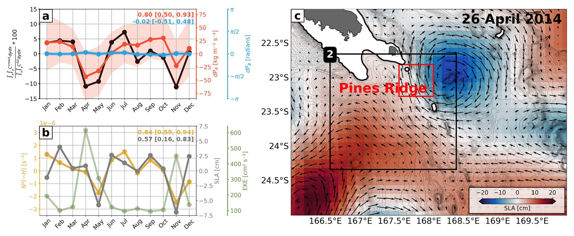
Figure 5 (a) Monthly time series of conversion anomaly (black) integrated over Pines Ridge (red box in c), expressed by the ratio $C^{\mathrm{cross}\mathrm{1}}/C^{\mathrm{D}\mathrm{2}}$. Also shown are the domain-averaged baroclinic bottom pressure amplitude (dP_A, red) and phase (dP_ϕ, blue) differences (including standard deviation). (b) Monthly time series of the domain-averaged bottom stratification (N²(−H), yellow) and mesoscale SLA (gray) and EKE (green). Mesoscale SLA, surface geostrophic velocity, and surface mesoscale EKE are computed similarly to Sect. 3.2 in Part 1. Briefly, we compute 5 d mean SSH to eliminate high-frequency variability before binning the data onto a $\mathrm{1}/\mathrm{4}$° horizontal grid. Finally, we applied a high-pass filter with the region's characteristic cut-off period of 180 d to account for the mesoscale. The correlation coefficients of (a) C^cross1 with dP_A and dP_ϕ and of (b) dP_A with N²(−H) for mesoscale SLA including their 90 % confidence intervals are also given. (c) The 5 d mean of mesoscale SLA, including the geostrophic velocity field, reveals a cyclonic eddy approaching Pines Ridge (red box).

Generalizing our results for the whole region is far from being straightforward. We calculate the probability density function of the correlation coefficients for the monthly time series of C^cross1 with dP_A, dP_ϕ, N²(−H), and mesoscale SLA for each subdomain (Fig. 6). The correlation coefficients for the domain-integrated/averaged quantities (filled circles) including their 90 % confidence intervals are also given. Generally, pressure amplitude variations are very pronounced, suggesting that local effects play an important role (Fig. 6a–d). Correlations with pressure phase variations tend to be less pronounced or more randomly distributed. Exempt therefrom is Norfolk Ridge (3), where pressure phase variations are strongly positively correlated, suggesting that remote effects are important (Fig. 6c). Note that pure correlations do not provide information about the amplitude of C^cross1. High correlations indicate that the temporal patterns of variability are consistent, but they do not imply that the magnitude of the conversion is equally significant across all regions.

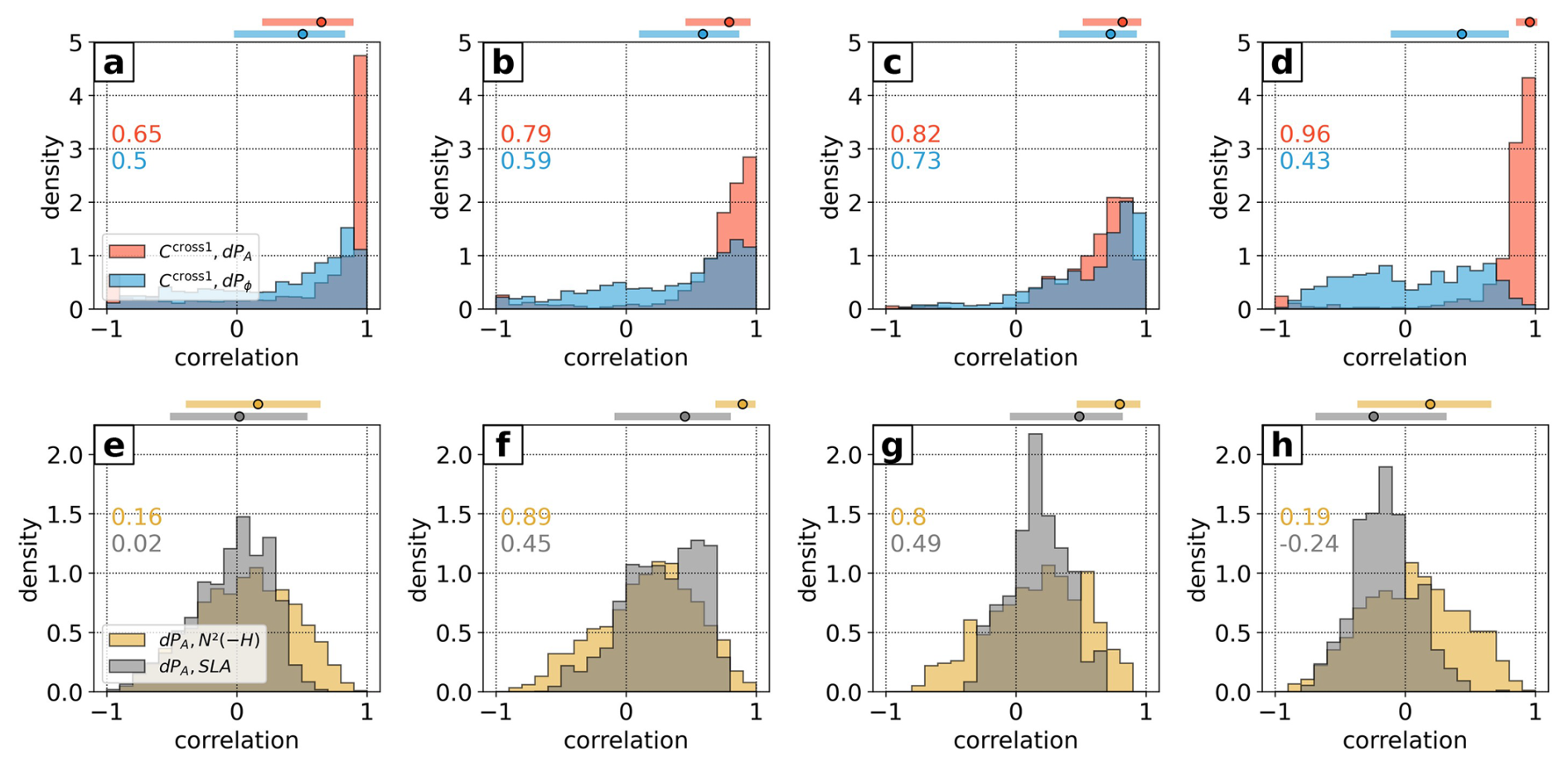
Figure 6 Histograms of the correlation coefficient between monthly averaged C^cross1 and incoherent baroclinic bottom pressure amplitude (dP_A, red) and phase (dP_ϕ, blue) differences for (a) North, (b) South, (c) Norfolk Ridge, and (d) Loyalty Ridge. We consider only regions where $\left|C^{\mathrm{D}\mathrm{2}}\right|>$ 0.2 W m⁻² to emphasize areas of strong conversion. (e–h) Same as above but for the correlation between dP_A and bottom stratification (N²(−H), yellow) and mesoscale SLA (gray). The correlation coefficients for the domain-integrated/averaged quantities (filled circles) including their 90 % confidence intervals are also given above the panels. The associated time series are explicitly shown in Fig. A2. Note that correlation coefficients based on the domain-integrated/averaged time series can largely differ from the probability distributions, as explained in Sect. 4.2.

Assuming that local effects dominate overall, the probability density functions for the correlation of pressure amplitude variations with bottom stratification and mesoscale SLA are shown in (Fig. 6e–h). In Fig. 6f and g (representative of the South (2) and Norfolk Ridge (3) domains), the slightly negatively skewed probability density functions are statistically robust with the hypothesis that conversion variations are linked with mesoscale-eddy-induced stratification changes. This becomes more evident when considering the correlation coefficients based on the area-integrated/averaged time series (see the filled circles above the panels). There are good correlations with bottom stratification (South (2): r=0.89 [0.71, 0.96]; Norfolk Ridge (3): r=0.80 [0.49, 0.93]) and mesoscale SLA (South (2): r=0.45 [−0.06, 0.78]; Norfolk Ridge (3): r=0.49 [−0.02, 0.79]). In these regions, mesoscale-eddy-induced stratification changes can induce semidiurnal conversion anomalies by up to 20 % relative to the coherent conversion (see also Fig. A2). These correlations (based on the area-integrated/averaged time series) can largely differ from the regional probability distributions, as the former may give greater weight to regions of enhanced conversion influenced by mesoscale variability. In contrast, the probability density functions represent the correlations at every grid point. We only choose grid points where $\left|C^{\mathrm{D}\mathrm{2}}\right|>$ 0.2 W m⁻² to emphasize areas of strong conversion. We note that as the threshold increases, the probability distributions become more negatively skewed, indicating increasingly positive correlations of dP_A with N²(−H) and mesoscale SLA (not shown).

North (1) and Loyalty Ridge (4) show no clear correlations between pressure amplitude variations with bottom stratification and mesoscale SLA (Fig. 6e and h). Several explanations are possible. First, the assumption of depth-independent or weakly baroclinic structure may not be valid. Particularly, conversion at Loyalty Ridge (4) takes place in deeper waters (1000–3000 m compared to < 1000 m in the South (2) domain) and is, thus, considerably deeper than the eddies' vertical extent. Mesoscale eddies near North (1) are generally less numerous and much less energetic than south of New Caledonia (Keppler et al., 2018). There are many other factors which can alter conversion such as seasonal stratification changes. Seasonal stratification changes have recently been reported to drive conversion variations on global scales (Kaur et al., 2024). In our study region, they seem to play a secondary role and are at best superimposed on mesoscale variability (see also Fig. A2). Other local processes include the direct influence of background currents, which induce asymmetries in internal-tide generation, being enhanced on the upstream side of bathymetric obstacles (Lamb and Dunphy, 2018; Shakespeare, 2020; Dossmann et al., 2020). Nonetheless, remote effects can play an essential role in local conversion variations, too. They primarily include the remotely generated internal tides, which undergo phase modulations as they propagate through the open ocean before impinging on bathymetric slopes; these are subject to local internal-tide generation. They are usually out of phase with the local tide forcing, though they can theoretically be in phase or in opposite phase as well, making it hard to distinguish local from remote effects. However, remote effects seem to be of relatively small importance around New Caledonia except at minor internal-tide generation sites, which lie in the propagation direction of the major tidal beams. Moreover, there are no major remote sources of internal tides which potentially shoal on the New Caledonia ridges.

We conclude that mesoscale variability can be an important source of conversion variations by enhancing/reducing semidiurnal energy conversion within the internal-tide generation hot spots around New Caledonia. Generalizing our findings is challenging since the relative importance of the underlying dynamics can strongly vary among the generation sites. Furthermore, many processes may be superimposed. Nonetheless, on monthly to intraseasonal timescales we attribute 10 %–20 % of semidiurnal conversion variations to mesoscale-eddy-induced stratification changes.

5 Mesoscale-eddy-induced refraction of tidal beams leads to increasing tidal incoherence in the far field

Once generated, semidiurnal internal tides propagate in narrow tidal beams. Within the generation hot spots, the variability of semidiurnal energy flux divergence is closely correlated with that of semidiurnal conversion and, thus, follows the spring–neap tide cycle (Fig. 2). In the annual mean, tidal incoherence of energy flux divergence can account for an important fraction, which stands in contrast to the conversion term (see Fig. 1f, Table 1). We will show in the following that tidal incoherence becomes increasingly important in the far field, linked to mesoscale eddy variability around New Caledonia. First, evidence is given by the monthly mean (July 2014) of $\left|{\mathit{F}}_{\mathrm{bc}}^{\mathrm{inc}}\right|$ and the surface geostrophic velocity field (Fig. 7a). In the influence area or in the propagation direction of the tidal beams, elevated incoherent energy levels > 10 kW m⁻¹ are clearly associated with intensified mesoscale currents. This suggests that the semidiurnal energy flux becomes incoherent as it propagates through the eddy field, especially south of New Caledonia where mesoscale EKE is enhanced (Fig. 7b). Reduced levels of incoherent energy fluxes north of New Caledonia correspond to weaker mesoscale surface currents.

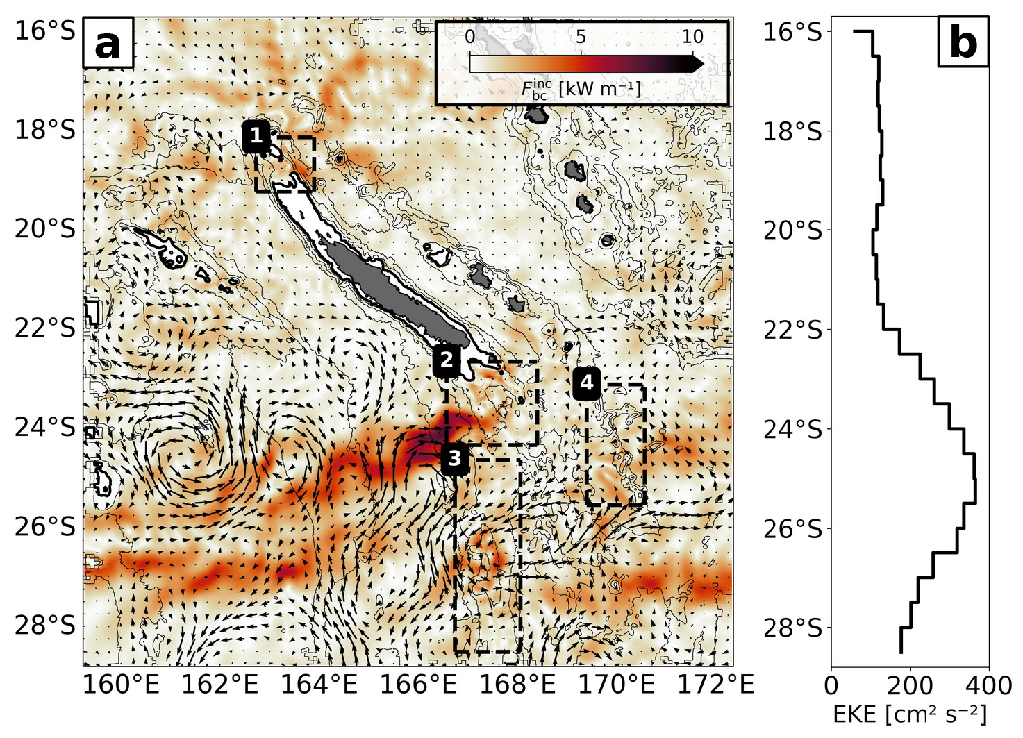
Figure 7 (a) Monthly mean (July 2014) semidiurnal incoherent energy flux ($\left|{\mathit{F}}_{\mathrm{bc}}^{\mathrm{inc}}\right|$) overlaid by the surface geostrophic velocity field representative of the mesoscale eddy field. (b) Zonally averaged mesoscale EKE (annual mean) as a function of latitude.

In the following, we apply a simplified ray tracing to quantify the refraction of tidal beams through mesoscale eddies, distinguishing between stratification and currents (see Sect. 2.3). The theoretical mode-1 ray paths for monthly averaged fields of stratification and/or currents are shown in Fig. 8. The reference ray path for annually averaged stratification and currents is also shown. The ray tracing yields profoundly different results for the tidal beam energy propagation north and south of New Caledonia (Fig. 8a). Theoretical rays initiated in the North (1) domain are confined narrow tidal beams, which closely align with the theoretical propagation direction for annually averaged stratification and currents. This stands in contrast to the theoretical rays initiated in the South (2) domain, experiencing notable refraction in the propagation direction (Table 3). The extent to which a semidiurnal ray is refracted by background stratification and/or currents is quantified by the cumulative refraction, for which we integrate absolute anomalies of the ray's propagation angle (computed from the group velocity vector). This anomaly is referenced to the propagation angle of the reference ray. This illustrates that rays are up to 5 times more refracted south of New Caledonia compared to north of New Caledonia (Table 3).

Table 3 Cumulative refraction anomaly relative to the reference ray (annually averaged stratification and currents) averaged over all semidiurnal rays for the first baroclinic mode initiated from the North (1) and South (2) domains for the three scenarios as in Fig. 8.

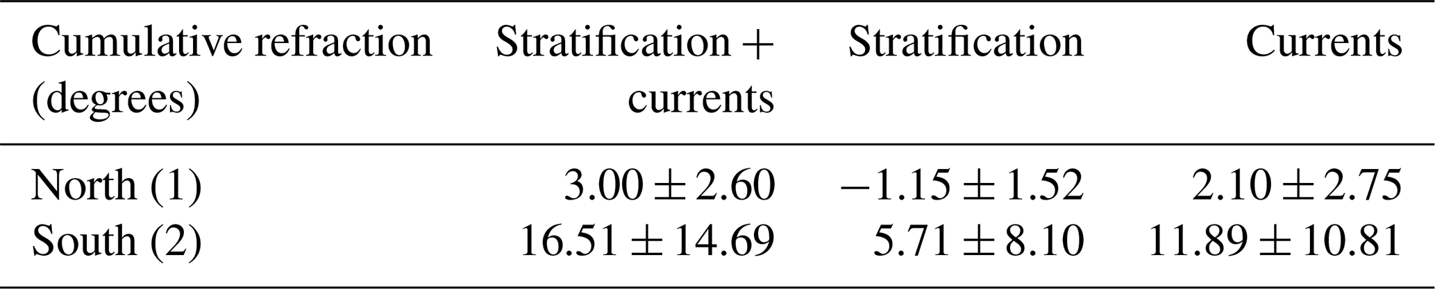
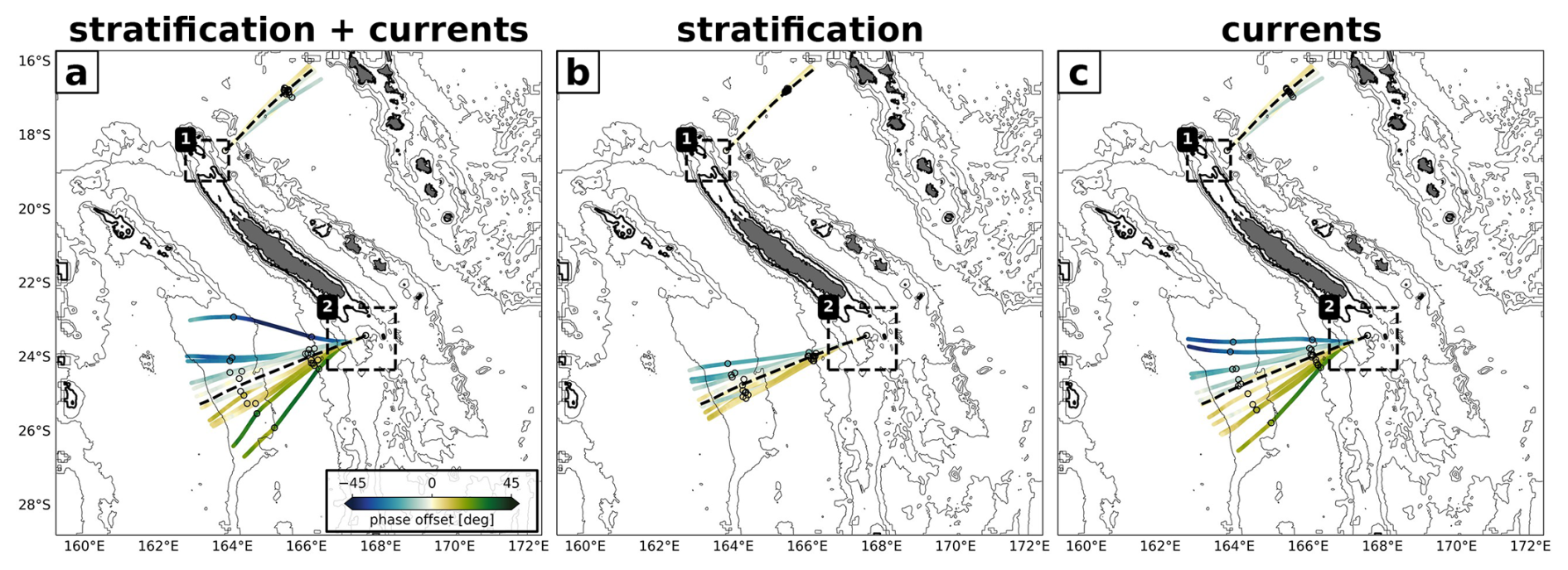
Figure 8 Modeled semidiurnal ray paths for the first baroclinic mode initiated at the northern (163.75° E, 18.4° S) and southern (167.65° E, 23.35° S) internal-tide generation sites of New Caledonia. Rays are computed using monthly varying and/or annually averaged fields of stratification and currents over a full calendar year. Refraction is shown for (a) monthly varying stratification and currents, (b) monthly varying stratification with annually averaged currents, and (c) monthly varying currents with annually averaged stratification. The reference ray, based on annually averaged stratification and currents, is also shown (dashed black line). The rays are further shown as a function of phase offset relative to the reference ray.

Mesoscale eddy activity is elevated south of New Caledonia, explaining the contrast between the North (1) and South (2) domains and to what extent a theoretical ray is being refracted (see Fig. 7b). The physical mechanism lies in the background currents and/or stratification-induced changes of the wave's group and phase speeds, which in turn cause the tidal beam to refract or change orientation, deviating from the propagation direction of the reference ray (Fig. 8a). Here, tidal beam refraction is dominated by mesoscale currents accounting for twice as much cumulative refraction along the propagation path compared to mesoscale stratification (Fig. 8b and c, Table 3). This is in agreement with recent findings (e.g., Guo et al., 2023). Overall, ray refraction by mesoscale currents leads to increasing dispersion in the far field, which is expressed inter alia in increasing phase variability.

6 Implications of tidal incoherence for SSH observability of balanced and unbalanced motions

Internal tides typically manifest in SSH as variations on the order of a few centimeters. In Part 1, the SSH signature of the coherent M₂ internal tide was analyzed. How the incoherent internal tide manifests in SSH remained to be investigated. These insights may provide crucial information for the dynamical interpretation of SSH measurements from satellite altimeter missions such as SWOT while helping disentangle contributions from balanced and unbalanced motions. This is especially important in regions where these dynamics have comparable temporal and spatial scales and contribute equally to SSH variance, such as New Caledonia.

The transition scale L_t is often used as a quantitative measure to estimate the length scale where unbalanced motions begin to dominate over balanced motions. L_t is commonly derived from one-dimensional SSH wavenumber spectra along altimeter tracks or two-dimensional spectra from numerical simulations, revealing strong geographic and seasonal variability. For instance, submesoscale processes are typically more energetic in winter months (Callies et al., 2015; Rocha et al., 2016), while internal tides often feature amplified SSH signatures in summer due to enhanced surface stratification (Lahaye et al., 2020; Kaur et al., 2024). However, these methods assume isotropy in the horizontal plane for the dynamics of interest. This is reasonable for mesoscale to submesoscale processes but not for internal tides with well-defined propagation directions, which potentially leads to biased interpretations.

In the following, we investigate the SSH imprint of the semidiurnal incoherent tide. Implications of tidal incoherence for SSH observability of balanced and unbalanced motions are deduced by computing SSH wavenumber spectra both in the direction of tidal energy propagation and along realistic altimetry tracks, and we explore the implications of tidal incoherence for the observability of balanced and unbalanced motions around New Caledonia.

6.1 Semidiurnal SSH decomposed into its coherent and incoherent parts

We extend the analysis in Sect. 2.2 by decomposing semidiurnal SSH into its coherent and incoherent parts (Fig. 9). The overall signature resembles the semidiurnal energy flux in Fig. 1d–f with the predominant beams to the north and south of New Caledonia, clearly visible in SSH with root mean square (rms) > 6 cm and dominated by the coherent tide (Fig. 9a–b). The SSH manifestation of the incoherent tide is characterized by an overall smaller but important rms (1–2 cm; Fig. 9c). The incoherent SSH is less confined to the tidal beams and seems more widespread in the domain, which suggests that the dispersion of internal waves occurs all along their propagation through the domain.

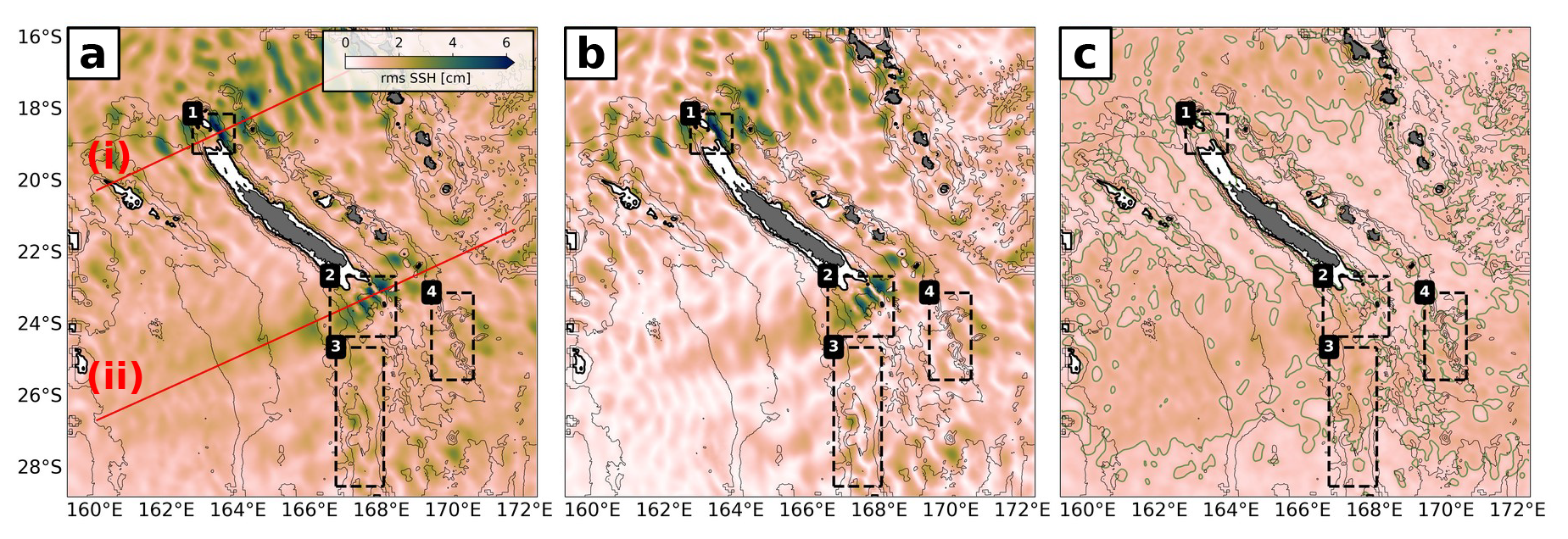
Figure 9 Annual root mean square (rms) of (a) semidiurnal SSH decomposed into the (b) coherent and (c) incoherent components. For the incoherent SSH, the 1 cm contour is shown (green). Bathymetry contours and the black boxes are given as in Fig. 1. The labels (i) and (ii) in panel (a) are the transects in the tidal energy propagation direction, which are used to compute SSH wavenumber spectra (see Sect. 6.2).

6.2 SSH wavenumber spectra in tidal beam energy propagation direction: an optimal case study

In Part 1, we calculated annually averaged SSH wavenumber spectra along the beam direction for two transects: (i) a northern transect and (ii) a southern transect (see Fig. 9a). The objective was to investigate the underlying dynamical regimes and assess the relative importance of balanced and unbalanced motions. The analysis revealed that the coherent internal tide strongly dominates SSH variance within the mesoscale band, limiting SSH observability of balanced motions to large eddy scales. By applying a correction for the coherent internal tide, it was shown that this observability can be increased by shifting the transition scale to smaller wavelengths.

Here, we revisit this analysis by addressing the incoherent internal tide to understand its impact on transition scales and potentially for SSH observability of balanced motions. Similarly to Part 1, we investigate SSH wavenumber spectra with regard to different dynamics that are separated in terms of frequency bands: subinertial frequencies (ω<f, SSH_subinertial) for mesoscale and submesoscale dynamics, as well as superinertial frequencies (ω>f, SSH_{superinertial}) for internal gravity waves, while distinguishing between the coherent internal tide (SSH_coh), incoherent internal tide (SSH_inc), and supertidal frequencies (ω> $\mathrm{1}/\mathrm{10}$ h, SSH_supertidal). Note that the incoherent internal tide is determined by applying a bandpass filter in the full semidiurnal–diurnal tidal range (10–28 h). As such, it also comprises contributions from near-inertial, non-tidal internal gravity waves and short-lived submesoscale features, but we assume that they are negligibly small.

Seasonally averaged SSH spectra for Southern Hemisphere summer (January–March, JFM) and winter (July–September, JAS) are shown in Fig. 10. By definition, the coherent internal tide is the same in both seasons. The seasonality of the transition scale corrected for the coherent internal tide ($L_{\mathrm{t}}^{\mathrm{corr}}$) is, thus, generally attributed to seasonal variations of subinertial motions, i.e., mesoscale to submesoscale dynamics, and unbalanced wave motions. First, we point out that the incoherent internal tide (SSH_inc) predominantly governs motions at superinertial frequencies if corrected for the coherent internal tide – at least down to 100 km independent of the season for both transects.

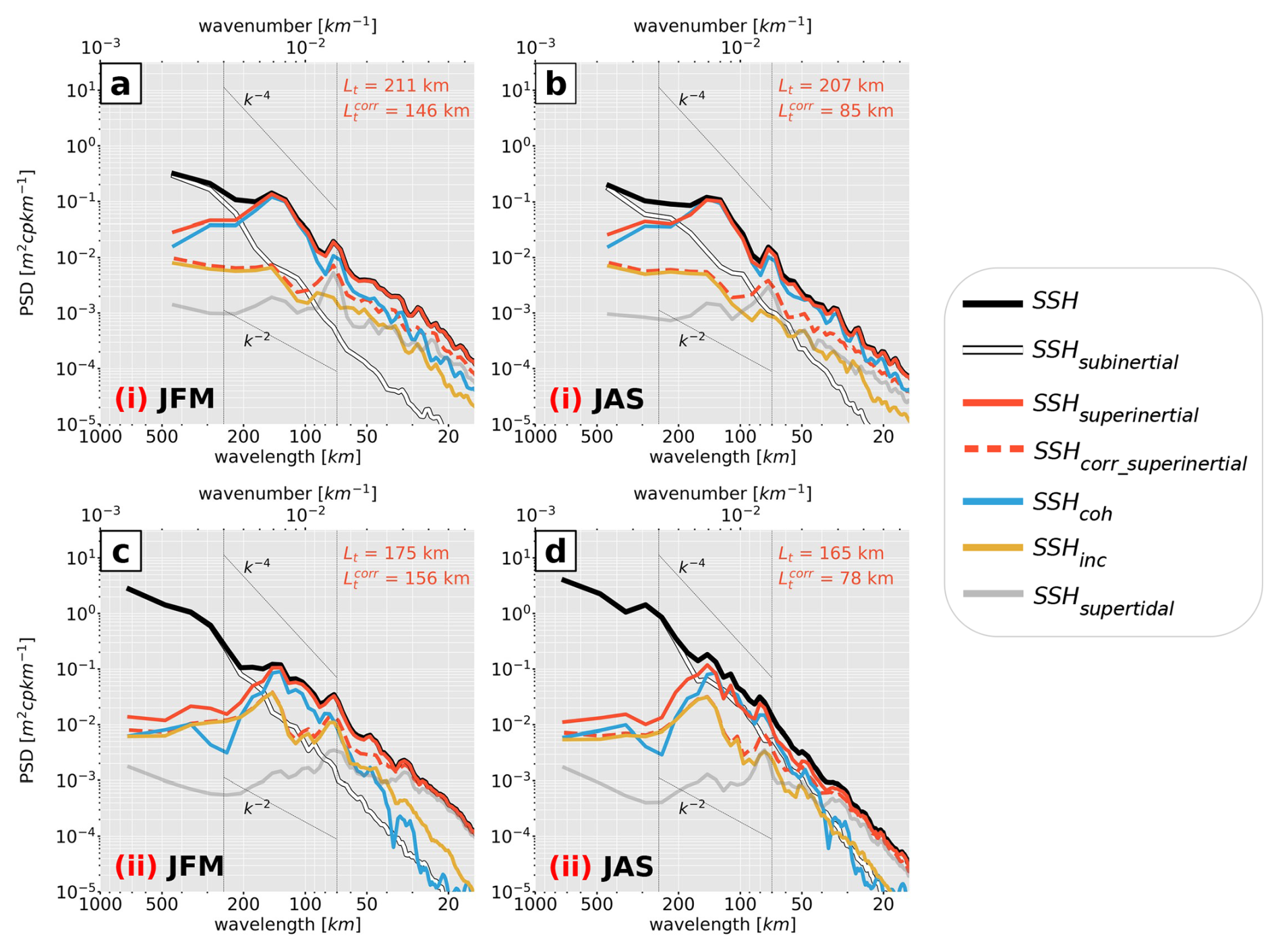
Figure 10 Seasonally averaged SSH wavenumber spectra, i.e., Southern Hemisphere summer (January–March, JFM) and winter (July–September, JAS), for transects (a–b) north and (c–d) south of New Caledonia, denoted as (i) and (ii), respectively, in Fig. 9a. SSH spectra are presented for the altimetry-like SSH (corrected for the barotropic tide, SSH, black) with regard to the different dynamics that are separated in terms of frequency bands: subinertial (ω < f, SSH_subinertial, white) for mesoscale and submesoscale dynamics, superinertial frequencies (ω>f, SSH_{superinertial}, solid red) for internal gravity waves decomposed into the coherent (SSH_coh, blue), incoherent (SSH_inc, yellow) internal tide, and supertidal frequencies (ω $>\mathrm{1}/\mathrm{10}$ h, SSH_supertidal, gray). The altimetry-like SSH corrected for both the barotropic and baroclinic tide and filtered for motions at superinertial frequencies (SSH_{corr_superinertial}, dashed red) is also given. The characteristic wavenumber slopes k⁻² and k⁻⁴ are represented by the dotted black lines encompassing the mesoscale band (70–250 km) (vertical dotted black lines). The transition scale L_t (i.e., where SSH_{superinertial}>SSH_subinertial) and the transition scale corrected for SSH_coh ($L_{\mathrm{t}}^{\mathrm{corr}}$, i.e., where SSH_{corr_superinertial}>SSH_subinertial) for the annually averaged SSH spectra are specified by the red numbers.

Along the southern transect, seasonal modulations of the SSH spectra become evident for all wavelengths < 300 km (Fig. 10c–d). In summer, it features a more flattened wavenumber slope in the mesoscale to submesoscale range with a characteristic k⁻² slope corresponding to superinertial motions (internal wave continuum) (Fig. 10c). In winter, it becomes more continuous, characterized by a k⁻⁴ slope (Fig. 10d). This can be attributed to subinertial motions such as mesoscale to submesoscale processes that undergo seasonal variability. This was explicitly shown for New Caledonia in Sérazin et al. (2020) and Bendinger (2023), in which increasing importance of mixed layer instabilities and frontogenesis was attributed to more available potential energy in the Southern Hemisphere winter months. Seasonal modulations of SSH spectra can also be linked to unbalanced wave motions, which are amplified in summer months, particularly for higher vertical modes due to increasing stratification (Lahaye et al., 2020; Kaur et al., 2024). Superinertial processes dominate subinertial motions in both seasons at scales below 180 km. However, the relative importance of superinertial over subinertial motions is more pronounced in summer months. This can be explained by the seasonality of superinertial and subinertial motions being out of phase; i.e., superinertial motions are enhanced in summer, while subinertial motions are considerably reduced and vice versa in winter. The transition scale (L_t) does not feature strong seasonality between summer and winter (Fig. 10c, d), though the transition scale is not well-defined in winter, where subinertial and superinertial signals have similar variance at wavelengths 90–180 km (Fig. 10d).

Important conclusions are made when correcting for the coherent internal tide. In summer, the transition scale ($L_{\mathrm{t}}^{\mathrm{corr}}$) is only slightly reduced from 175 to 156 km (Fig. 10c). This is linked to the seasonally enhanced incoherent internal tide, which is still contained in the signal featuring equal SSH variance with subinertial signals at 90–180 km wavelength (Fig. 10c). At scales below 90 km, the incoherent tide even dominates SSH variance over subinertial motions and is equally important to the coherent tide. In winter, the transition scale is largely reduced from 165 to 78 km (Fig. 10d). This is primarily linked to the fact that subinertial motions are energized in winter, while the SSH signature of motions at superinertial frequencies are less energetic. We note a significant contribution of motions at supertidal frequencies for scales smaller than 100 km.

The northern domain differs from the southern domain in that SSH variance of subinertial motions is generally reduced and the seasonal cycle less pronounced (shown by the white lines in Fig. 10a–b). Motions at superinertial frequencies largely dominate over motions at subinertial frequencies throughout the year, dominated by the coherent internal tide. As for the southern transect, the incoherent contribution features seasonality and increases in summer but remains weaker than the coherent signal. Increasing SSH observability of mesoscale and submesoscale motions by correcting for the coherent internal-tide signal proves overall to be more efficient since the incoherent internal-tide signal is largely reduced in SSH variance compared to the southern transect (Fig. 10a–b). Specifically, the transition scale is reduced from 211 to 146 km in summer (Fig. 10a) and from 207 to 85 km in winter (Fig. 10b). Contributions by motions at supertidal frequencies appear to have larger importance in the northern domain compared to the southern domain. In fact, at scales below 146 and 85 km for summer and winter, respectively, SSH variance is governed by equal contributions from the incoherent internal tide and motions at supertidal frequencies.

Briefly summarized, the dominance of unbalanced motions in the mesoscale to submesoscale band strongly limits SSH observability of geostrophic dynamics around New Caledonia, especially in summer. In other words, SSH observability of mesoscale dynamics is limited to large eddy scales even after a correction for the coherent tide in numerical simulation output. It is to a large extent the incoherent internal tide and non-tidal internal gravity waves at scales < 100 km which may eventually constrain SSH observability of mesoscale and submesoscale dynamics.

6.3 SSH wavenumber spectra in along-track direction: a satellite altimetry perspective

The SSH wavenumber spectra in Fig. 10 and the associated conclusions for transition scales are only valid for a one-dimensional transect in the tidal beam propagation direction, in which the internal-tide signature is well-captured. Here, we mimic SSH wavenumber spectra from satellite altimetry by interpolating SSH from CALEDO60 (similarly to Sect. 6.2) onto realistic altimetry tracks, which are not aligned with the tidal beam propagation direction (Fig. 11). Further, the SSH wavenumber spectra are averaged for the region south of New Caledonia (Fig. 11a).

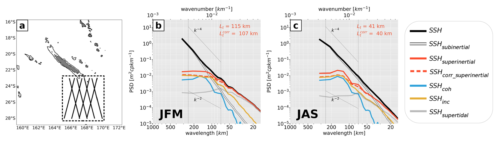
Figure 11 Same as in Fig. 10, but for CALEDO60 SSH interpolated onto satellite ground tracks, which reassemble those of SWOT, and averaged over the region south of New Caledonia as shown by the highlighted tracks in (a), distinguishing between (b) summer and (c) winter months.

South of New Caledonia and along the tidal beam propagation direction, the coherent tide was found to clearly dominate over subinertial motions or to be of comparable importance, regardless of the season (see Fig. 10c–d). However, averaged SSH wavenumber spectra along given altimetry tracks reveal a different picture. Spectral peaks associated with tidal motions are less pronounced (Fig. 11b–c). L_t is generally decreased from 175 to 115 km in summer months and from 165 to 41 km in winter months. This reduction is linked to the anisotropic nature of the (coherent) internal tide. Along the altimetry track direction, only a fraction of the internal-tide energy is captured, causing the SSH wavenumber spectra to emphasize the more isotropic balanced flow regime. Moreover, the incoherent internal tide becomes increasingly important, dominating over the coherent tide across all spatial scales. This shift reflects the larger isotropy of incoherent SSH compared to the coherent SSH. Consequently, in along-track spectra, the dominance of balanced motions and the incoherent internal tide renders corrections for the coherent tide ineffective. This is evident when comparing L_t and $L_{\mathrm{t}}^{\mathrm{corr}}$ in Fig. 11b and c (from 115 to 107 km in summer months and 41 to 40 km in winter months).

We conclude that the orientation of altimetry tracks has important implications for the interpretation of transition scales computed on along-track SSH wavenumber spectra. This effect is particularly pronounced in regions with prominent internal-tide motion and well-defined propagation beams, such as around New Caledonia. In such cases, transition scales may lead to erroneous estimates of the wavelength at which unbalanced motion becomes dominant over balanced motion, as anisotropic motions like internal tides are not effectively captured in the along-track direction. Separating balanced from unbalanced motions is critical for the dynamical interpretation of SWOT SSH, particularly for accessing the mesoscale to submesoscale flow regime and derived quantities such as surface geostrophic velocities.

7 Summary and perspectives

New Caledonia, an archipelago in the southwestern tropical Pacific, is a semidiurnal internal-tide generation hot spot as revealed by numerical simulation output from a regional model (Bendinger et al., 2023) and in situ observations (Bendinger et al., 2024). This region is of particular interest for the SWOT altimeter mission since internal tides coexist with the mesoscale to submesoscale circulation. Being subject to potential eddy–internal-tide interactions, New Caledonia represents a challenge for SWOT SSH observations. In this study, we investigated the temporal variability of the semidiurnal internal tide, not previously considered in Bendinger et al. (2023). Based on hourly numerical simulation output of a full model calendar year, a bandpass-filtering technique, and harmonic analysis, we decomposed the depth-integrated semidiurnal barotropic-to-baroclinic conversion, energy flux, and dissipation (residual) into their coherent and incoherent parts. These findings are summarized below.

7.1 Tidal incoherence in the near field

In the annual mean, semidiurnal barotropic-to-baroclinic conversion is largely dominated by the coherent tide, which in turn explains a large part of the semidiurnal variability (90 %–99 %) through the spring–neap cycle. The incoherent tide is negligibly small in the annual mean, suggesting that incoherent contributions cancel out in the long-term average, though locally and on shorter timescales, it can explain a notable fraction of semidiurnal variability. Our objective was to identify the underlying mechanisms responsible for conversion variations not linked to the tidal forcing.

Generally speaking, sources of conversion variations are numerous and difficult to distinguish due to the unpredictable nature of local and remote effects. To clearly distinguish between these dynamics, we separated the incoherent conversion C^inc into its purely incoherent term ($C^{{\mathrm{inc}}^{*}}$) and two cross-terms (C^cross1, C^cross2) (see Eq. 5). Our analysis suggests that the work done by the coherent barotropic tide on incoherent baroclinic bottom pressure variations dominates incoherent conversion (71 %–90 %), expressed by C^cross1. The dominance of baroclinic bottom pressure amplitude variations (over phase variations) implies that local effects dominate over remote effects. Locally and on monthly to intraseasonal timescales, mesoscale-eddy-induced stratification changes through upward (CE) and downward (AE) pumping of isopycnal surfaces can induce negative and positive conversion anomalies by more than 20 %, respectively. This is supported by positive correlations of incoherent baroclinic bottom pressure amplitude variations with bottom stratification and mesoscale SLA. Seasonal variability seems to play a minor role or is superimposed on the dominant mesoscale variability. The importance of conversion variations through changes in the barotropic tide forcing remains to be investigated, but we showed that they can explain an important fraction of up to 23 % in the incoherent conversion term.

7.2 Tidal incoherence in the far field

Semidiurnal tidal energy propagating towards the open ocean follows at first order the spring–neap tide cycle, closely coupled to semidiurnal conversion variability. However, it features elevated levels of tidal incoherence, which increases with increasing distance from the generation sites. Close to the generation sites, tidal incoherence explains up to 20 % of the semidiurnal variability. In the far field, it can account for up to 90 % (in 500–1000 km distance from the generation site). Tidal incoherence is generally of higher importance south of New Caledonia, corresponding to enhanced mesoscale activity, leading to dispersion in the far field alongside increasing phase variability. Further, it is associated with the refraction of the tidal beams in the propagation direction. This is in agreement with a simplified ray tracing, which tracks the horizontal propagation of inertia-gravity modes at semidiurnal frequency with varying background stratification and/or currents. Tidal beam refraction occurs through varying group and phase speeds as the semidiurnal rays interact with the mesoscale eddy field. Changing orientation is primarily dominated by background currents accounting for twice as much refraction along the propagation path as stratification. North of New Caledonia, the semidiurnal rays closely align with the theoretical propagation direction for a semidiurnal ray in annually averaged stratification and currents.

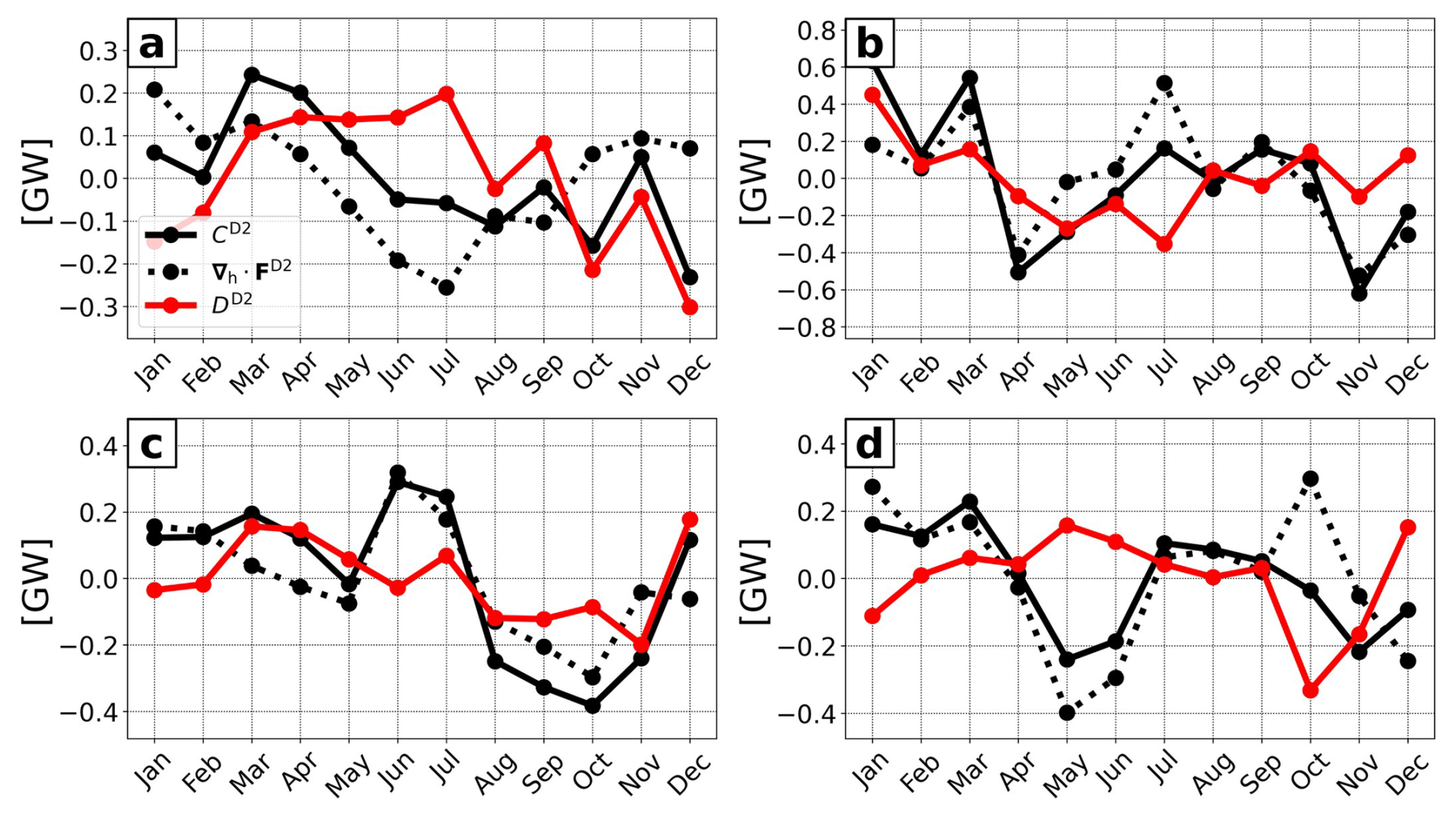
Figure 12 Monthly time series of semidiurnal barotropic-to-baroclinic conversion C^D2 and energy flux divergence ${\mathbf{\nabla }}_{\mathrm{h}}\cdot {\mathit{F}}_{\mathrm{bc}}^{\mathrm{D}\mathrm{2}}$, as well as $D_{\mathrm{bc}}^{\mathrm{D}\mathrm{2}}$ anomalies relative to the annual mean, integrated over (a) North, (b) South, (c) Norfolk Ridge, and (d) Loyalty Ridge.

7.3 Incoherent tide SSH limits SSH observability of mesoscale to submesoscale motions

The dynamical interpretation of SSH in regions where balanced and unbalanced motions feature similar SSH variance at comparable wavelengths is challenging. By revisiting Part 1, we computed SSH wavenumber spectra in the tidal energy propagation direction and extended the analysis by investigating the relative importance of the incoherent tide in SSH variance. A correction of the coherent tidal signature in SSH is only partly effective in accessing scales toward smaller wavelengths due to seasonal modulations of superinertial and subinertial motions, which are in opposite phase; i.e., superinertial motions are enhanced in summer, while subinertial motions are considerably reduced and vice versa in winter. Ultimately, it is the incoherent tide which limits SSH observability of balanced and unbalanced motions to scales above 150 km in summer and above 80 km in winter.

SSH wavenumber spectra computed along altimetry tracks lead to several conclusions. The altimetry tracks are not oriented in the tidal energy propagation direction, and therefore the spectra capture only part of the internal-tide energy. The incoherent tide dominates over the coherent tide across all wavelengths, reflecting its more isotropic nature compared to the coherent tide. Moreover, transition scales derived along altimetry tracks are generally reduced compared to those determined in the tidal energy propagation direction since the SSH wavenumber spectra emphasize the more isotropic balanced flow regime. Relying on these transition scales in regions where balanced and unbalanced motions coexist may result in a distorted view of the governing dynamics as anisotropic processes such as internal tides are not properly sampled. However, knowing at which wavelengths balanced and unbalanced motions dominate is particularly crucial for SWOT in order to disentangle the different flow regimes in SSH measurements.

7.4 Perspectives of this work

This study provides several routes for future work to better understand the internal-tide life cycle. One open question arising from our analysis is how variability in barotropic-to-baroclinic energy conversion influences both the outward propagation of internal-tide energy and local dissipation. According to the baroclinic energy budget (Eq. 1), dissipation is defined as the residual between conversion and energy flux divergence. We therefore ask the following question: do variations in conversion directly translate into proportional changes in energy flux divergence – and, by extension, in dissipation – or are they partially decoupled? For instance, does increased conversion always imply stronger outward flux and higher dissipation (Falahat et al., 2014a)? Monthly anomalies of C^D2, ${\mathbf{\nabla }}_{\mathrm{h}}\cdot {\mathit{F}}_{\mathrm{bc}}^{\mathrm{D}\mathrm{2}}$, and $D_{\mathrm{bc}}^{\mathrm{D}\mathrm{2}}$ relative to the annual mean are shown in Fig. 12. Energy flux divergence anomalies generally follow those of conversion, with positive conversion anomalies typically resulting in increased energy flux divergence, and vice versa. In contrast, dissipation anomalies are less variable. Nevertheless, periods exist when energy flux divergence anomalies are either more or less pronounced than conversion anomalies, leading to reduced or enhanced dissipation, respectively. The processes governing whether an excess or a deficit of tidal energy conversion is balanced primarily by outward energy propagation or by local dissipation (or other terms in Eq. 1) remain to be fully understood.

This highlights the need for further investigation into the mechanisms controlling energy partitioning between these pathways. Those findings could have important implications for parameterizations of internal-tide dynamics such as tidal mixing and dissipation for climate and ocean general circulation models, which do not resolve tidal processes. Current parameterizations consider geographically varying tidal mixing (Vic et al., 2019; de Lavergne et al., 2019, 2020). However, temporal variations induced by the spring–neap cycle, mesoscale variability, and seasonal changes are not taken into account.

Further insight is expected from an extensive in situ experiment (SWOTALIS, Cravatte et al., 2024) that was carried out in March–May 2023. It was inter alia dedicated to the deployment of full-depth oceanographic moorings and located in the hot spots of internal-tide generation and dissipation south of New Caledonia. Successfully recovered in November 2023, these moorings provide a unique dataset to better understand the internal-tide life cycle, while assessing our numerical model output. Furthermore, this region is located beneath the two swaths of SWOT's fast sampling phase (1 d repeat orbit). The moorings and the numerical simulation output will play an essential role in the dynamical interpretation of SWOT SSH by allocating the different dynamics such as balanced and unbalanced motions. Emphasis will be given to the SSH signature of the incoherent internal tide, which represents a major challenge for SWOT SSH observability.

Appendix A

The hypothesis of conversion variations driven by mesoscale-eddy-induced stratification changes (see Sect. 4.2) is further supported below. We illustrate how mesoscale eddies, AE and CE, may affect the bottom stratification at the internal-tide generation site. Two examples, shown in Fig. A1, illustrate the presence of either an AE (Fig. A1a) or a CE (Fig. A1b) above Norfolk Ridge (3). These features are represented by positive and negative monthly averaged sea level anomalies (SLAs) for July and August, respectively. The zonal sections of the corresponding isopycnals indicate mesoscale-eddy-induced downward and upward pumping. The resulting stratification changes are depicted in zonally averaged stratification profiles (gray: annual mean; red: July; blue: August).

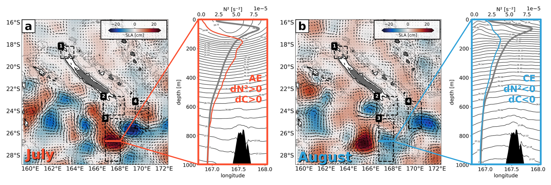
Figure A1 Monthly averaged mesoscale SLA for (a) July and (b) August qualitatively showing the impact of mesoscale variability on stratification and conversion through downward and upward pumping induced by AE and CE, respectively. The pumping is illustrated by the isopycnals along a zonal section trough the AE and CE. The zonal mean stratification profile for the given month (red: July; blue: August), as well as the annual mean (gray), is also shown.

In July, the AE causes downward pumping of isopycnals, leading to positive stratification anomalies near the seafloor (Fig. A1a). Conversely, in August, the CE induces upward pumping of isopycnals, which results in negative stratification anomalies near the seafloor (Fig. A1b). It is noteworthy that the stratification anomalies just above the seafloor (at approximately 800 m depth) are significantly smaller than those in the water column above. However, they consistently align with the overall sign of the stratification anomaly.

The monthly time series of the area-integrated conversion anomaly including domain-averaged baroclinic bottom pressure amplitude and phase variations as well as bottom stratification and mesoscale SLA and EKE for each subdomain are shown in Fig. A2. In the South (2) and Norfolk Ridge (3) domains, the above hypothesis is strengthened by the positive correlation coefficients (Fig. A2b and c). Even though we primarily link conversion variations to mesoscale variability, the monthly time series partly suggest seasonal variations of conversion. It tends to be enhanced in summer months and reduced in winter months corresponding to seasonally varying stratification. Regardless, mesoscale variability clearly enhances, suppresses, or even reverses the seasonally driven anomalies. A clear distinction between seasonally driven and mesoscale-driven stratification changes is needed in future work to allocate the exact contribution to conversion variations.

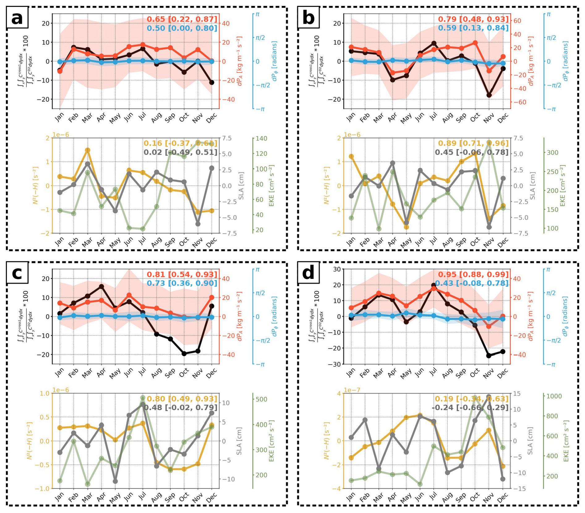
Figure A2 Monthly time series of the area-integrated conversion anomaly (black) induced by C^cross1 expressed by the ratio of C^inc and C^D2, domain-averaged baroclinic bottom pressure amplitude (dP_A, red) and phase (dP_ϕ, blue) difference between the semidiurnal and coherent tide (including standard deviation), domain-averaged bottom stratification (N²(−H), yellow), and mesoscale SLA (gray) and EKE (green) for (a) North (1), (b) South (2), (c) Norfolk Ridge (3), and (d) Loyalty Ridge (4). The correlation coefficients of C^cross1 with dP_A and dP_ϕ and of dP_A with N²(−H) for mesoscale SLA including their 90 % confidence intervals are also given.